
Unambiguous ISAR Imaging Method for Complex Maneuvering Group Targets

1
Air and Missile Defense College, Air Force Engineering University, Xi’an 710051, China
2
Science College, Armed Police Engineering University, Xi’an 710051, China
*
Author to whom correspondence should be addressed.
Remote Sens. 2022, 14(11), 2554; https://doi.org/10.3390/rs14112554
Submission received: 21 April 2022
/
Revised: 18 May 2022
/
Accepted: 25 May 2022
/
Published: 26 May 2022
(This article belongs to the Special Issue Radar and Sonar Imaging and Processing Ⅲ)
Abstract
:In inverse synthetic-aperture radar (ISAR) imaging, it is essential to deal with the Doppler ambiguity of group targets with complex maneuvers in order to avoid the bias of target position towards the actual value. Simultaneously, migration through resolution cell (MTRC) under the Doppler ambiguity is unable to be compensated for as a preprocessing. Traditional ISAR imaging methods for maneuvering targets, however, are undesirable to handle the severe deformation and defocusing in the imaging results induced by the Doppler ambiguity and MTRC. In this paper, we propose a novel and effective ISAR imaging method to improve the imaging quality by removing the Doppler ambiguity and compensating for the MTRC. Specifically, we first model the echo as a multi-component cubic phase signal (m-CPS) and design a high-order instantaneous autocorrelation function–generalized scaled Fourier transform (HIAF–GSCFT) to process the echo. This is to estimate the rotational parameters without MTRC compensation. Then, a maximum weighted contrast algorithm is used to remove the Doppler ambiguity, followed by reconstructing the echo. Compared with the existing method, the proposed method can accurately estimate the rotational parameters under the existing MTRCs and achieves a high-quality ISAR image for group targets, with complex maneuvers without Doppler ambiguity. Experiments of simulated and measured datasets validate its effectiveness and robustness for single target and group targets.
1. Introduction
In traditional ISAR imaging algorithms for maneuvering targets, the difficulty of achieving high-quality imaging results for complex maneuvering group targets is mainly caused by Doppler ambiguity because the Doppler frequency of partial scattering centers exceeds the limit of radar pulse repetition frequency (PRF). For group targets, the Doppler ambiguity generally exists among marginal subtargets, thus yielding the following two problems:
- It results in the difficulty of correcting migration through resolution cell (MTRC) [1] for accurate target rotation parameters estimation. Without the Doppler ambiguity, MTRC can be compensated for by methods such as Keystone [1], and only the Doppler diffusion caused by the higher-order phase is considered. In general, the echo of maneuvering targets can be seen as multi-component linear frequency modulation (LFM) signals in the slow-time domain [2]. ISAR imaging methods for LFM signals can be categorized into two types: time–frequency analysis methods, such as Wigner–Ville distribution [2,3,4], Radon–Wigner transform [5,6], and LV’s distribution (LVD) [7,8], and parameter estimation methods, such as matched Fourier transform (MFT) [9,10] and Chirp–Fourier transform [11,12]. With improvement in the maneuverability of the air targets, the echo can be further modeled as m-CPS [13,14]. Most ISAR imaging methods for m-CPS are based on parameter estimation, including cubic phase function (CPF) [15,16,17,18], high-order ambiguity function (HAF) [19,20,21,22,23], and discrete polynomial phase transformation (DPT) [24]. In recent years, some scholars proposed novel methods based on other well-performing time–frequency distributions [25,26,27]. With the Doppler ambiguity, however, MTRCs can no longer be effectively compensated for by the aforementioned methods. This will further cause difficulty in estimating the echo parameters to compensate rotational motion of targets. Therefore, it is of critical value to design an effective parameter estimation algorithm without corrected MTRC.
- Scattering centers with Doppler ambiguity will appear in an incorrect position [28,29], which highlights the necessity of removing the Doppler ambiguity. To our best knowledge, however, few studies focus on dealing with this issue. Dr. Huang and Dr. Zhang [30] presented a hypothesis that Doppler ambiguity removal can be carried out by sparse reconstruction. However, their proposed method has limited effectiveness for the m-CPS model.
In this study, we propose a novel ISAR imaging method to obtain an unambiguous ISAR imaging result of complex maneuvering group targets. In this method, the echo parameters are estimated to compensate for the rotational motion of targets by high-order instantaneous autocorrelation function–generalized scaled Fourier transform (HIAF–GSCFT), and a maximum weighted contrast (MWC) based algorithm is used to remove the Doppler ambiguity. The echo is then reconstructed to achieve unambiguous ISAR imaging. Experimental results prove that our method has better performance for complex maneuvering targets with MTRCs and Doppler ambiguity than traditional methods and is robust with different SNRs.
2. Materials and Methods
2.1. Signal Model
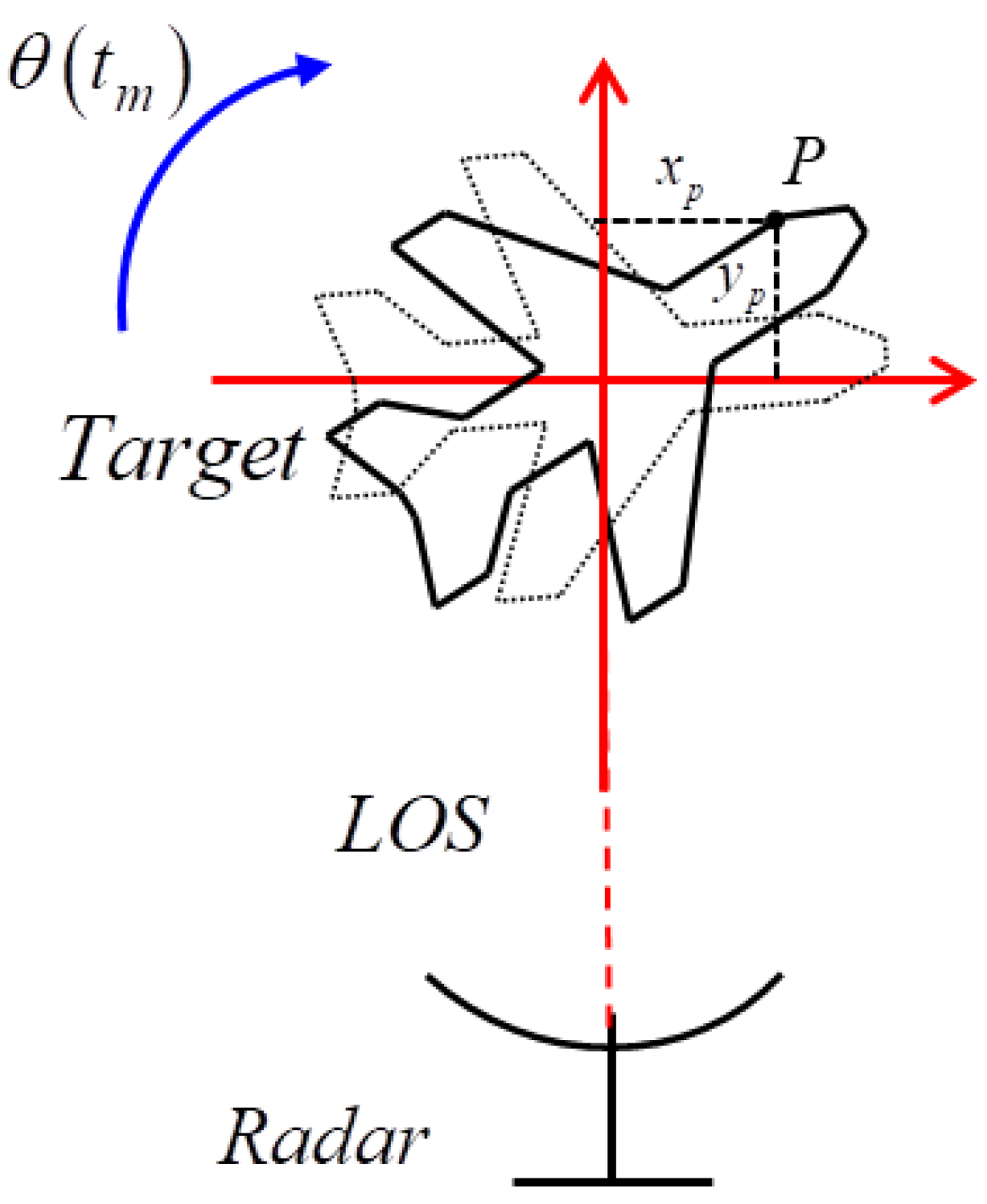
Generally, the movement of a target consists of translation and rotation. Since in this research, we mainly discuss rotational motion compensation, in this section, we directly analyze the echo after translational motion compensation. In this case, the turntable model of ISAR imaging is shown in Figure 1.
We set the transmitted signal as a linear frequency modulation signal
where is the pulse width, is the fast time, is the carrier frequency, is the chirp rate, is the total time, and is the slow time, with an integer multiplying the pulse repetition period.
After the stretch processing [31], the echo of the scattering center p is
where is the bandwidth, and is the fast time–frequency defined by
where is the reference range, and is the light speed.
Given that the target performs complex maneuvers, the rotation angle of the scattering center p is
where is the angular velocity of rotation, is the angular acceleration, and is the second-order angular acceleration.
Based on planar wavefront approximation that is reasonable for ISAR imaging, in Equation (2) can be expressed as
where and represent the Y–X coordinates of p, respectively, in the coordinate system in Figure 1.
Here, Equation (5) can be approximated by Taylor series expansion as
For the simplicity of notation, Equation (6) is written as
where , , , and .
Considering the influence of Doppler ambiguity, the echo signal of complex maneuvering group targets containing N scattering centers is
where is the number of Doppler ambiguity [30], and is the wavelength.
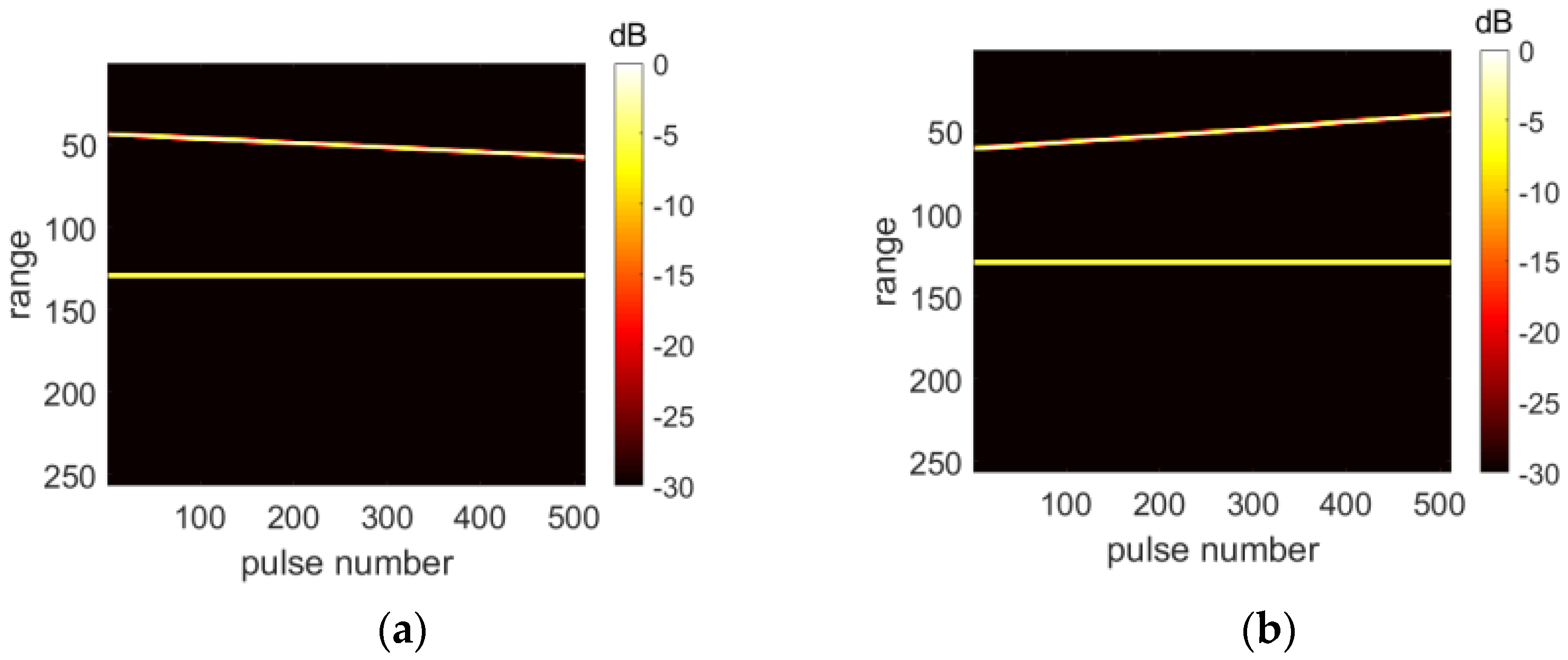
It is worth noting that the Doppler ambiguity shifts the unique correspondence between the azimuth information of the scattering centers and its Doppler frequency. In other words, scattering centers with the same Doppler frequency may also have different MTRC slopes, as shown in Figure 2.
In Figure 2a, the position of the scattering center with MTRC is and . In contrast, the position of the scattering center in Figure 2b is and . Although with the same Doppler frequency, the MTRC slopes of these two scattering centers are completely different, making the traditional MTRC correction method fail to achieve an ideal result.
2.2. Parameters Estimation Based on HIAF–GSCFT
Due to Doppler ambiguity, the echo parameters estimation needs to be carried out when the MTRC cannot be compensated for. Thus, HIAF–GSCFT is designed to estimate the echo parameters. Inspired by the autocorrelation function [32], we define HIAF as
where and are two delay constants. It is worth noting that and should be interpolated for the sake of the same number of sampling points. Combined with Equation (8), Equation (9) can be written as
where represents the cross-terms created by HIAF. In Equation (10), we ignore because in HIAF and phase separation, is invariant.
To ensure that GSCFT can effectively estimate the parameters, the phases only related to need to be eliminated. We define this process as phase separation (PS), which can be expressed as
where is the corresponding time variable of after inverse Fourier transform, represents the Fourier transform in , represents the inverse Fourier transform in , and represents the conjugate operation of the result after IFT.
After PS, the echo phase is
where is the cross-terms processed by PS.
According to [15] and [33], GSCFT is defined as
where represents the zoom factor to avoid spectrum aliasing, is the scaled frequency domain with respect to , and are constant power, is a function of , and is an empirical parameter.
According to Equation (12), the symbol in Equation (13) can be replaced by
To this end, the result of GSCFT is
where is the cross-terms processed by GSCFT.
Clearly, the first term of Equation (16) on the right side achieves energy focusing in domain, and the positions of the peaks are only related to . After inverse Fourier transform in domain, can be expressed as
In Equation (17), the echo of each individual scattering center has formed a peak on the domain. Simultaneously, the cross-terms cannot achieve energy accumulation through HIAF–GSCFT (see a detailed analysis of the cross-term in Appendix A). Therefore, the peak detection to estimate and is defined by
where and represent the coordinates of the maximum value, respectively.
Moreover, GSCFT, , and can also be used to estimate and . We first compensate for the higher-order phase of the dominant scattering center and perform PS by
where represents the echo components of nondominant scattering centers.
After GSCFT and Fourier transform, becomes
where is processed by GSCFT and Fourier transform (detailed analysis is provided in Appendix A).
Similarly, peak detection is used to obtain and by
In order to ensure the accuracy of parameter estimation, we use a grid-searching manner for in .
2.3. Doppler Ambiguity Removal Based on MWC
Given the Doppler ambiguity, the relationship between and the actual value is
where is the Doppler ambiguity number of the dominant scattering center.
MWC is thus proposed to determine . We first construct Equation (26) to multiply with the echo and transform the result into the domain
where is used to determine .
In Equation (27), when , the MTRC will be completely compensated for. In this case, the image quality of is better than .
To prevent the interference caused by the nondominant scattering centers, we define the weighted contrast as
where is the weighting coefficient defined by
where is proportional to the standard deviation of the data in each range cell.
Now, the dominant scattering center is moved to the middle of and has a larger weight than the other scattering centers. Thus, can be determined by the maximum of by
and the estimated Doppler frequency is
2.4. ISAR Imaging Method Based on HIAF–GSCFT and Doppler Ambiguity Removal
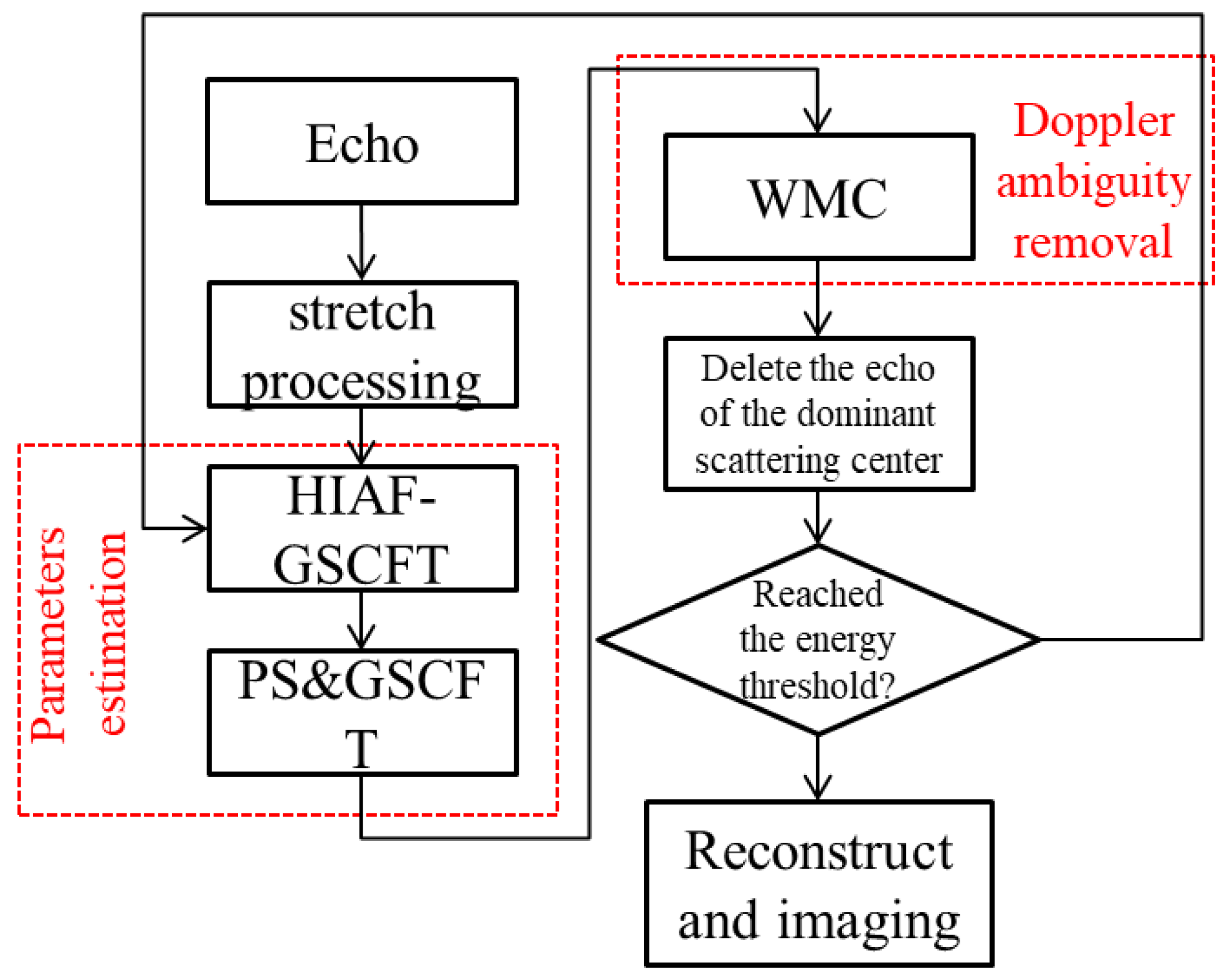
In this section, a HIAF–GSCFT- and MWC-based ISAR imaging method is introduced for complex maneuvering group targets with the following procedure:
- Step 1
- Obtain by processing the original echo signal using stretch processing;
- Step 2
- Estimate and using HIAF–GSCFT;
- Step 3
- Estimate and with PS, GSCFT, inverse Fourier transform, and the compensation function constructed by the estimated echo parameters;
- Step 4
- Remove the Doppler ambiguity by using the MWC and determine the actual Doppler frequency of the dominant scattering center;
- Step 5
- Estimate the amplitude of the dominant scattering center by the least-squares method as
- Step 6
- Delete the echo of the dominant scattering center from as
- Step 7
- Repeat steps (2)–(6) till the residual energy of the echo reach the energy threshold;
- Step 8
- Reconstruct the echo by
Eventually, we interpolate the slow time grid and perform a 2D Fourier transform on to obtain an ISAR imaging result as
The flowchart of the proposed method is shown in Figure 3.
3. Results
In this section, we verify the proposed method from three aspects: the performance of parameter estimation, the capability of single target imaging, and the effectiveness of imaging for complex maneuvering group targets.
3.1. Validation of the Parameters Estimation Method Based on HIAF–GSCFT
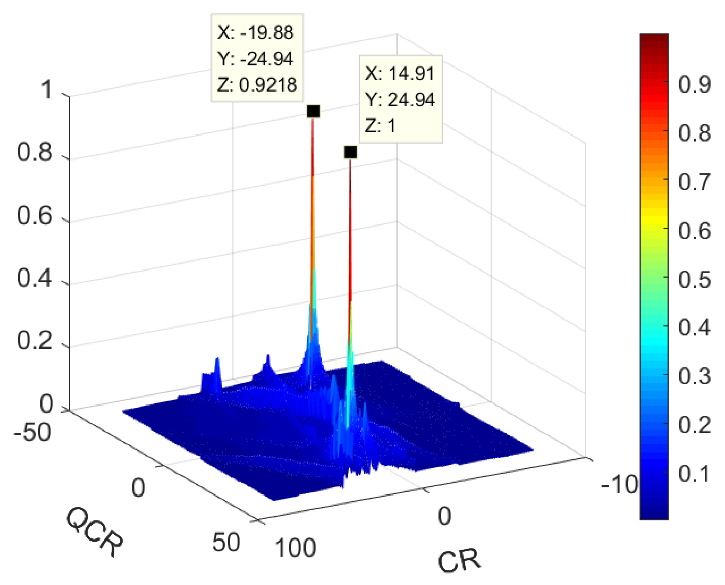
As an m-CPS has two components, its signal model is similar to (8), and the rotational parameters are set as
Component 1: , , , ;
Component 2: , , , .
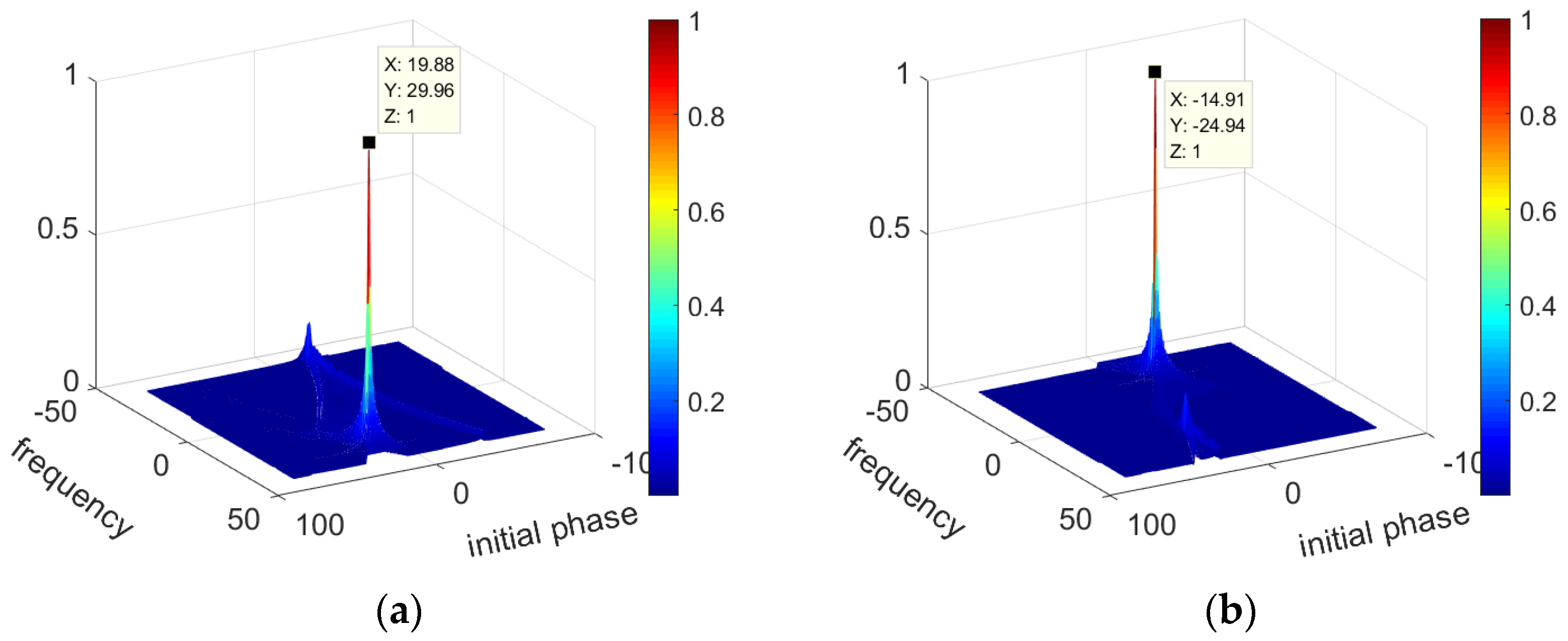
After HIAF–GSCFT for the m-CPS, the result is shown in Figure 4.
In Figure 4, CR and QCR represent the chirp rate and the quadratic chirp rate, respectively.
The two components achieve two individual energy accumulation. According to Figure 4, we estimate the parameters as , , , and , corresponding to relative estimation errors as 0.6%, 0.24%, 0.6%, and 0.24%, respectively. This is caused by discrete sampling intervals. Considering the small scale, however, these errors can be ignored.
Using the estimated parameters to compensate for the high-order phases of component 1 and component 2, respectively, and perform GSCFT, the results under two compensation cases are shown in Figure 5.
In Figure 5a, only component 1 achieves effective energy focusing because its high-order phases are compensated for correctly. Thus, we have and . Similarly, the frequency and the initial phase of component 2 can be estimated from Figure 5b as and respectively. The relative errors of these estimated parameters are 0.6%, 0.24%, 0.6%, and 0.24%, respectively.
From these results, it is fundamental that our proposed HIAF–GSCFT-based parameter estimation method has a strong capability of achieving accurate parameter estimation of m-CPS, with high-order coupling between and .
3.2. Validation of the Capability of Single Target Imaging
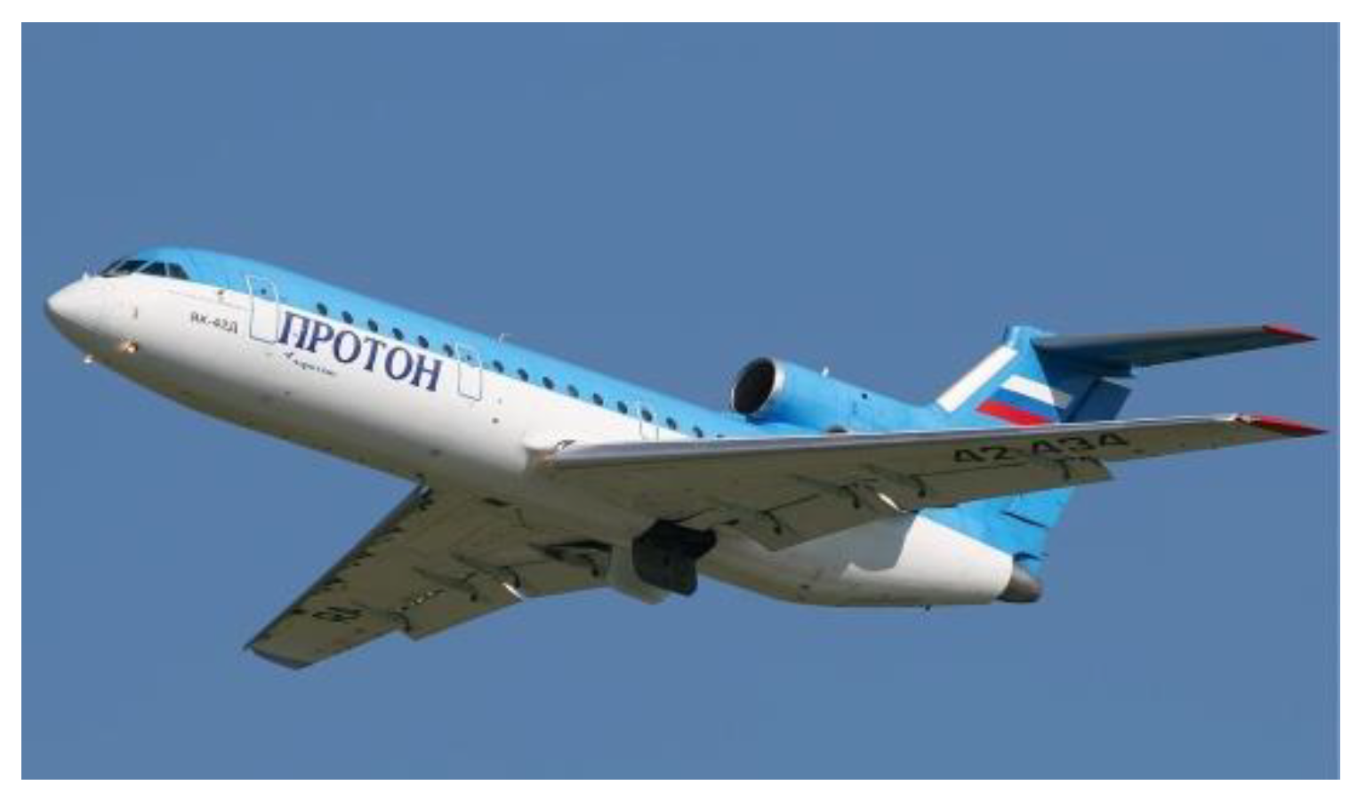
We adopted Yak-42 measured data to validate the imaging ability for a single target of the proposed method. The outline of Yak-42 is shown in Figure 6.
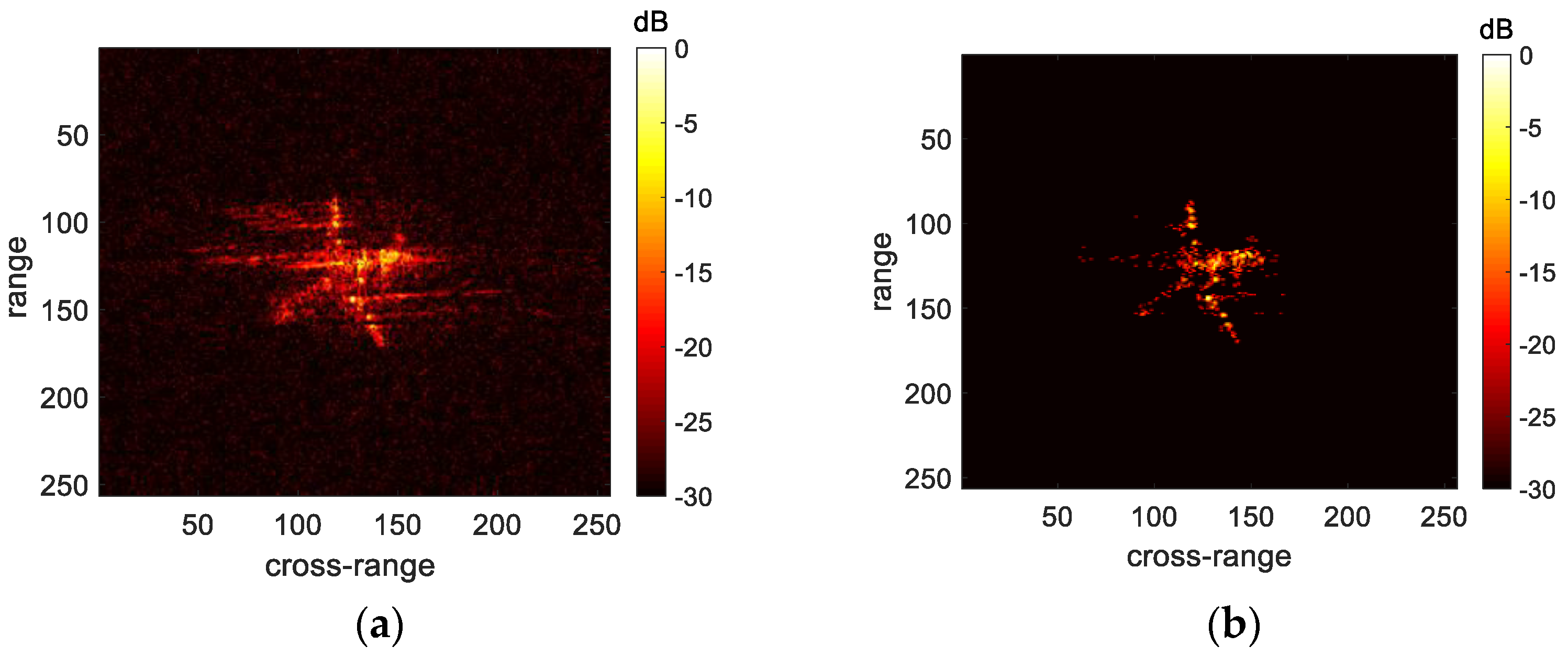
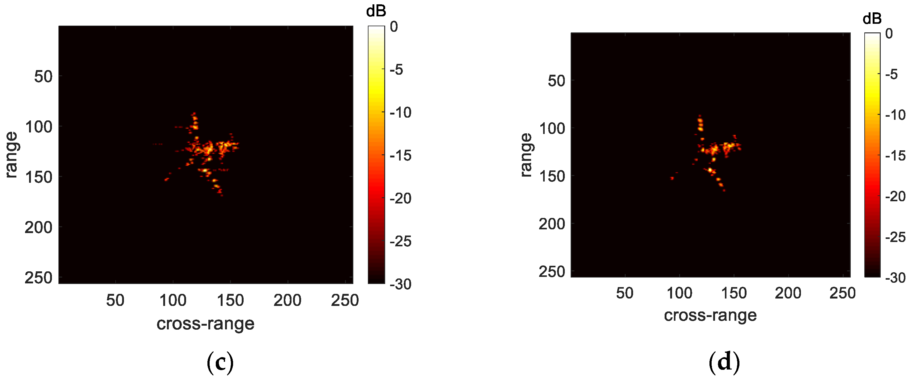
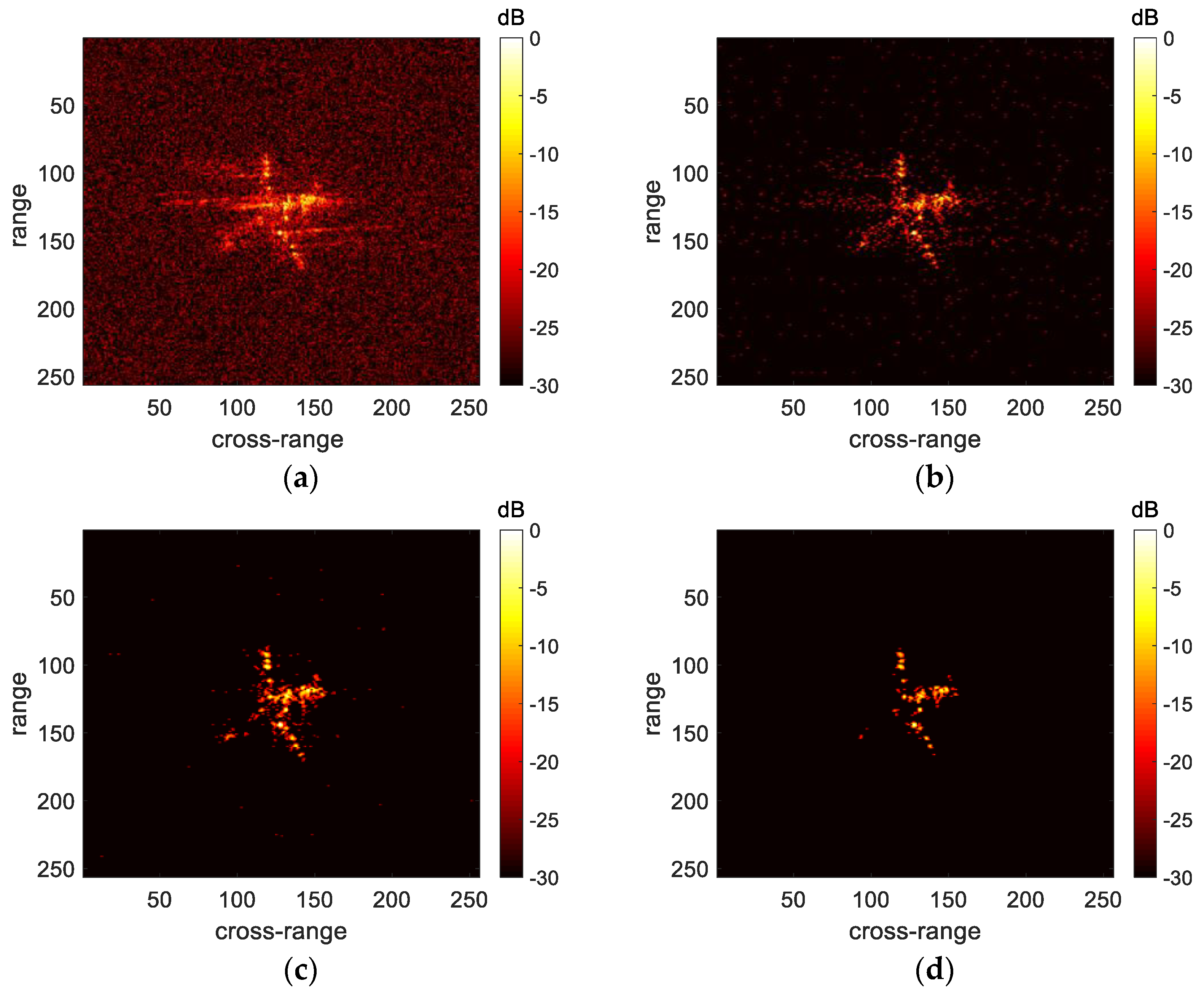
Parameters of the radar are 5.52 GHz carrier frequency, 100 Hz pulse repetition frequency, and 400 MHz bandwidth. We added white Gaussian noise (SNR = 5 dB and 0 dB) and MTRC to the data and compared our proposed method with range-Doppler (RD) [1], HAF–ICPF [21], and integrated parametric cubic phase function-reversing Wigner–Ville distribution (IPCPF–RWVD) [15], where RD is a classical ISAR imaging algorithm, HAF–ICPF is an effective imaging method for complex maneuvering target, and IPCPF–RWVD is a robust imaging method for a complex maneuvering target. The results of the above four methods are in Figure 7 and Figure 8.
Specifically, the RD method was severely defocused, especially on the body and wings of the aircraft. The HAF–ICPF method slightly improved the imaging quality, but the scattering centers of the body were still defocused. The IPCPF–RWVD method had better performance than HAF–ICPF because the IPCPF–RWVD method had a lower degree of nonlinearity. However, the result of the IPCPF–RWVD method was still defocused because MTRC affects the accuracy of parameter estimation. In contrast, our method effectively overcame the negative influence of MTRC in parameter estimation and obtained clear imaging results, as shown in Figure 7d and Figure 8d. In summary, this experiment proved the strong ability for high-quality ISAR imaging for a single target when MTRC is uncalibrated.
3.3. Validation of Imaging for Complex Maneuvering Group Targets
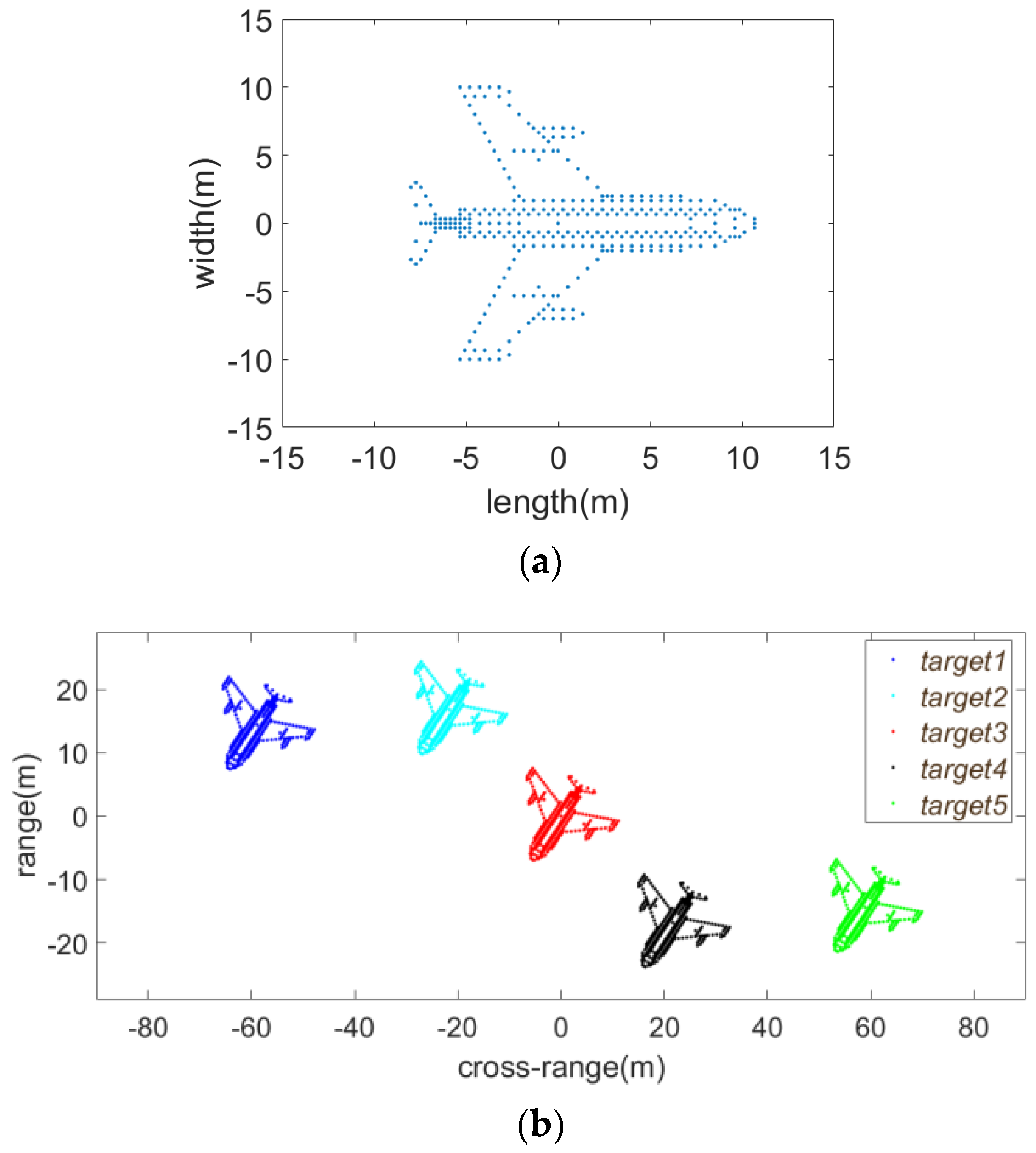
Next, we used synthetic data to validate the effectiveness of the proposed method for complex maneuvering group targets. As shown in Figure 9a, the simulated aircraft consists of 330 scattering centers, with a length of 18.67 m and a wingspan of 24 m. The amplitude of the scattering centers obeys the Rayleigh distribution, with . The group targets were composed of five simulated aircraft, and the spatial distribution is given in Figure 9b.
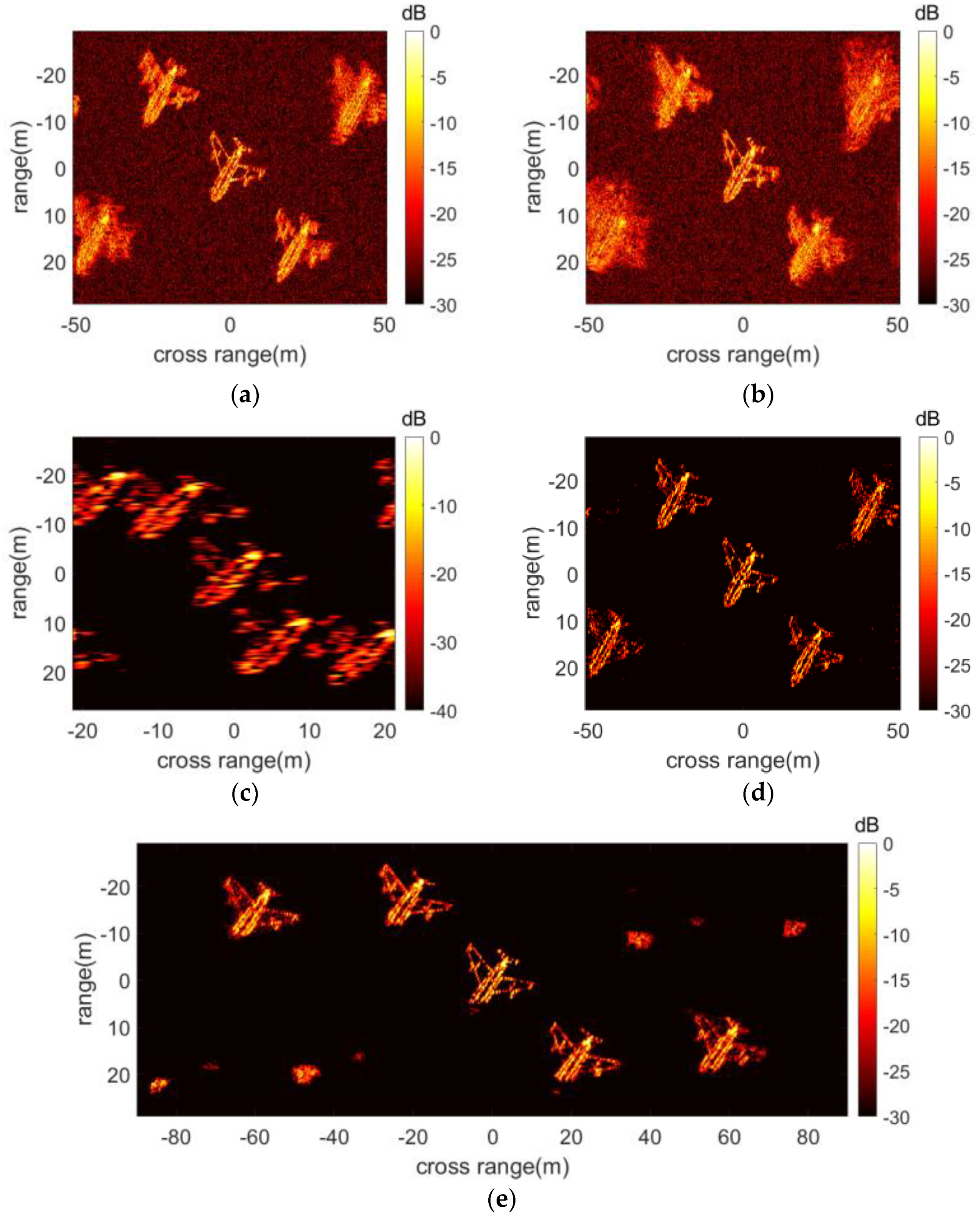
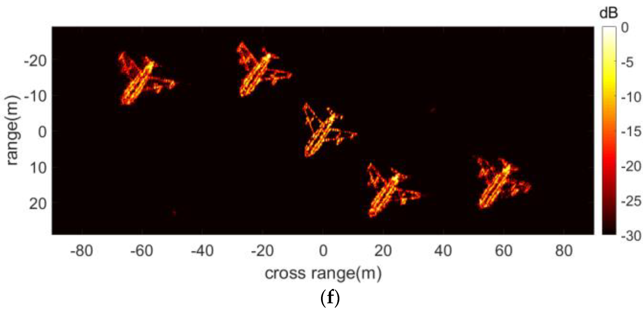
For SNR = 5 dB, the ISAR imaging result obtained with the proposed method is shown in Figure 10f. In comparison, the results by RD, RD–Keystone, SPWVD, and HAF–ICPF, as well as the results reported in [30], are provided in Figure 10a–e, respectively. SPWVD is an effective imaging method for the LFM signal model, and the method in [30] is an imaging method for group targets.
When using the RD method, the Doppler ambiguity resulted in targets 1 and 5 appearing in the wrong positions, and the results were completely defocused. The result of RD–Keystone was even worse than RD because Keystone is invalid with MTRC under the Doppler ambiguity. SPWVD and HAF–ICPF methods improved the imaging results at different but limited levels of target defocusing; however, they did not have any effects on removing the Doppler ambiguity. The method in [30] was unable to remove the Doppler ambiguity of every scattering center because [30] is not ideal when applied to the m-CPS model. In contrast, our proposed method completely eliminated the Doppler ambiguity and defocus, as shown in Figure 10f. In summary, the proposed method effectively achieved the best quality imaging result for complex maneuvering group targets among all of the compared methods.
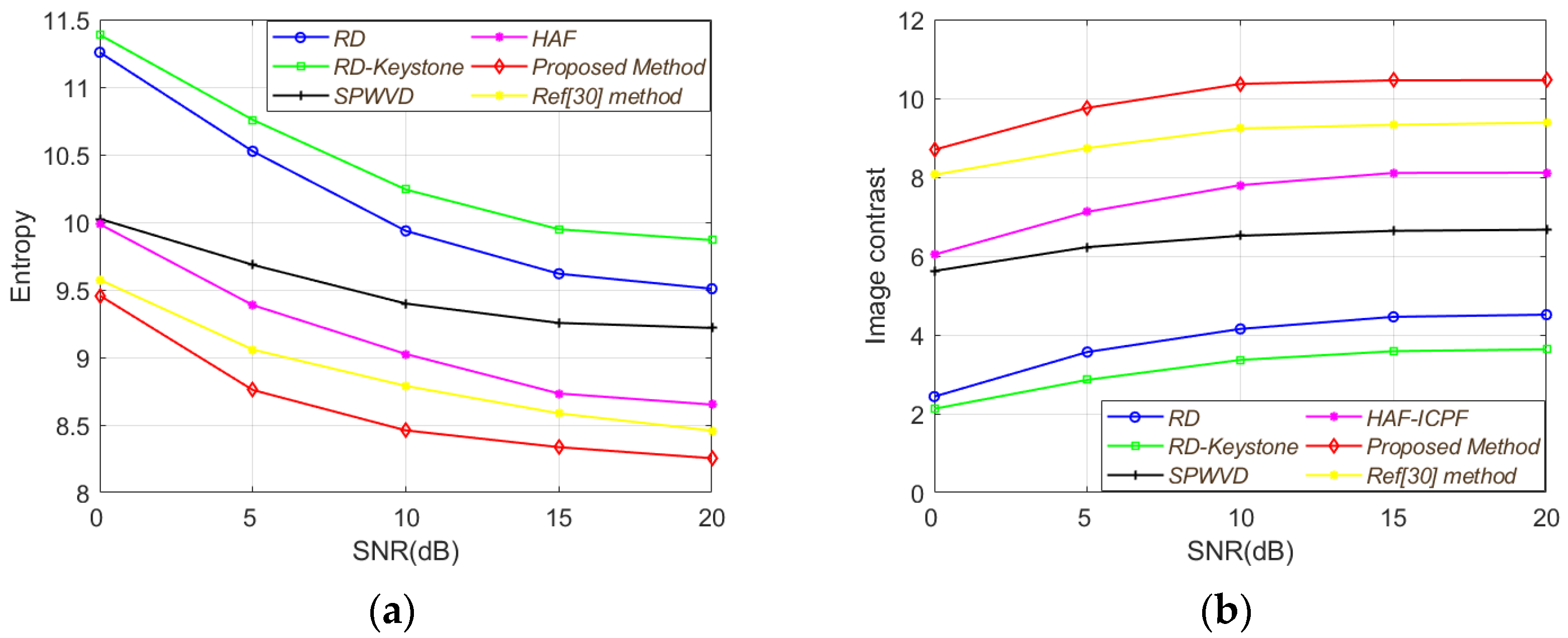
Finally, we validated the imaging quality of the proposed method under different SNRs. We adopted entropy and contrast to measure the quality of imaging results. After 50 Monte Carlo experiments, the SNR versus entropy curves and SNR versus contrast curves of the above six methods were drawn, which are shown in Figure 11.
We found that the imaging quality of RD and RD–Keystone were invalid. This is because the two methods were unable to compensate for the influence caused by the nonuniform rotation. SPWVD and HAF had better performance than the above two methods but were still not ideal because of the existence of Doppler ambiguity and MTRC. The performance of the method in [30] was the closest to that of the proposed method. However, the method was unable to correct the Doppler ambiguity of complex maneuvering group targets. In comparison, the imaging quality of our proposed method is significantly superior to all the other methods with different SNRs. This experiment effectively revealed the robustness of our method against different noise levels.
4. Conclusions
In this research, we presented a novel and effective ISAR imaging method for complex maneuvering group targets. In this method, the echo parameters were estimated via HIAF–GSCFT, and the MWC algorithm was used to remove the Doppler ambiguity. The proposed method effectively estimated rotational parameters in the presence of MTRC and improved the accuracy of Doppler ambiguity removal. Moreover, our method could be applied for complex maneuvering group targets. Experimental results demonstrated the effectiveness and robustness of this method with different SNRs. In future research, we plan to further improve the proposed method, by reducing the nonlinearity of the algorithm to improve the algorithm’s noise robustness and reduce the computational complexity.
Author Contributions
D.H. provided research ideas, F.L. completed simulation experiments and thesis writing, X.G. refined and polished the manuscript, and C.F. performed the final proofreading of the manuscript. All authors have read and agreed to the published version of the manuscript.
Funding
This work was supported by the National Postdoctoral Science Foundation of China under grant 2019M661508, Shaanxi Provincial Fund Youth Project of China under grant 2019JQ-497 and Aviation Science Fund of China under grant 201920096001 (Funder: Darong Huang). The APC was funded by 2019JQ-497.
Data Availability Statement
The data presented in this study are available on request from the corresponding author. The data are not publicly available due to the request of the funder.
Acknowledgments
This research was supported by the National Postdoctoral Science Foundation of China under Grant 2019M661508, Shaanxi Provincial Fund Youth Project of China under Grant 2019JQ-497, and Aviation Science Fund of China under Grant 201920096001.
Conflicts of Interest
The authors declare no conflict of interest.
Appendix A
In this section, we conduct a detailed analysis of the changes in the cross-terms and nondominant echo components during the HIAF–GSCFT process. In Equation (17), we give three different forms of the components below.
where p, q, r, and s are four different scattering centers on the target. When they are used as the subscripts of a parameter, it represents that the parameter belongs to the echo of the corresponding scattering center. , and are written in Equation (A4), respectively.
In Equation (21), is given by
For two different scattering centers p and q in the imaging scene, their position relationship should at least satisfy or . Combining Equation (6), the parameters of p and q satisfy at least or and are subject to and . Furthermore, we can obtain , , while . After PS processing, the signal models of the cross terms and nondominant echo components can be summarized into by
According to Equation (13), the prerequisite for using GSCFT to achieve energy focusing is that must be related to only. In Equation (A6), however, is coupled with and . Moreover, the high-order phase of prevents the signal from forming a peak through inverse Fourier transform. In summary, the cross-term and the nondominant echo components cannot achieve energy focusing through GSCFT and Fourier transform, indicating that they have no effects on the parameter estimation.
References
- Xing, M.; Wu, R.; Lan, J.; Bao, Z. Migration Through Resolution Cell Compensation in ISAR Imaging. IEEE Geosci. Remote Sens. Lett. 2004, 1, 141–144. [Google Scholar] [CrossRef]
- Berizzi, F.; Mese, E.; Diani, M.; Martorella, M. High-resolution ISAR imaging of maneuvering targets by means of the range instantaneous Doppler technique: Modeling and performance analysis. IEEE Trans. Image Process. 2001, 10, 1880–1890. [Google Scholar] [CrossRef] [PubMed]
- Barbarossa, S. Analysis of multicomponent LFM signals by a combined Wigner-Hough transform. IEEE Trans. Signal Process. 1995, 43, 1511–1515. [Google Scholar] [CrossRef]
- Wang, Y.; Jiang, Y. ISAR Imaging of Maneuvering Target Based on the L-Class of Fourth-Order Complex-Lag PWVD. IEEE Trans. Geosci. Remote Sens. 2010, 48, 1518–1527. [Google Scholar] [CrossRef]
- Wood, J.; Barry, D. Radon transformation of time-frequency distributions for analysis of multicomponent signals. IEEE Trans. Signal Process. 1994, 42, 3166–3177. [Google Scholar] [CrossRef]
- Li, W.-C.; Wang, X.-S.; Wang, G.-Y. Scaled Radon-Wigner Transform Imaging and Scaling of Maneuvering Target. IEEE Trans. Aerosp. Electron. Syst. 2010, 46, 2043–2051. [Google Scholar] [CrossRef]
- Yang, T.L.; Yang, L.; BI, G. ISAR cross-range scaling algorithm based on LVD. In Proceedings of the 2016 39th International Conference on Telecommunications and Signal Processing (TSP), Vienna, Austria, 27–29 June 2016; pp. 643–664. [Google Scholar]
- Li, X.L.; Cui, G.L.; Kong, L.J. Fast Non-Searching Method for Maneuvering Target Detection and Motion Parameters Esti-mation. IEEE Trans. Signal Process. 2016, 64, 2232–2244. [Google Scholar] [CrossRef]
- Guo, B.; Sun, H.; Yin, W.; Zeng, H.; Chen, G.; Deng, L. ISAR Imaging Algorithm of Maneuvering Target Based on Matching Flourier Transform. In Proceedings of the 2018 IEEE 4th International Conference on Computer and Communications (ICCC), Chengdu, China, 7–10 December 2018; pp. 1710–1714. [Google Scholar] [CrossRef]
- Wang, Y.; Zhang, Q.; Zhao, B. ISAR imaging of target with complex motion based on novel approach for the parameters estimation of multi-component cubic phase signal. Multidimens. Syst. Signal Process. 2018, 29, 1285–1307. [Google Scholar] [CrossRef]
- Wang, B.; Xu, S.; Wu, W.; Hu, P.; Chen, Z. Adaptive ISAR Imaging of Maneuvering Targets Based on a Modified Fourier Transform. Sensors 2018, 18, 1370. [Google Scholar] [CrossRef] [Green Version]
- Zuo, L.; Wang, B. ISAR Imaging of Non-Uniform Rotating Targets Based on Optimized Matching Fourier Transform. IEEE Access 2020, 8, 64324–64330. [Google Scholar] [CrossRef]
- O’Shea, P.J. A Fast Algorithm for Estimating the Parameters of a Quadratic FM Signal. IEEE Trans. Signal Process. 2004, 52, 385–393. [Google Scholar] [CrossRef] [Green Version]
- O’Shea, P. Improving Polynomial Phase Parameter Estimation by Using Nonuniformly Spaced Signal Sample Methods. IEEE Trans. Signal Process. 2012, 60, 3405–3414. [Google Scholar] [CrossRef]
- Lv, Q.; Su, T.; He, X. An ISAR Imaging Algorithm for Nonuniformly Rotating Targets with Low SNR Based on Modified Bilinear Parameter Estimation of Cubic Phase Signal. IEEE Trans. Aerosp. Electron. Syst. 2018, 54, 3108–3124. [Google Scholar] [CrossRef]
- Zheng, J.; Liu, H.; Liu, Z.; Liu, Q.H. ISAR Imaging of Ship Targets Based on an Integrated Cubic Phase Bilinear Autocorrelation Function. Sensors 2017, 17, 498. [Google Scholar] [CrossRef] [Green Version]
- Zhu, L. Quadratic Frequency Modulation Signals Parameter Estimation Based on Product High Order Ambiguity Func-tion-Modified Integrated Cubic Phase Function. Information 2019, 10, 140. [Google Scholar] [CrossRef] [Green Version]
- Li, L.; Yan, L.; Li, D.; Liu, H.; Zhang, C. A Novel ISAR Imaging Method for Maneuvering Target Based on AM-QFM Model Under Low SNR Environment. IEEE Access 2019, 7, 140499–140512. [Google Scholar] [CrossRef]
- Wang, Y.; Kang, J.; Jiang, Y. ISAR Imaging of Maneuvering Target Based on the Local Polynomial Wigner Distribution and Integrated High-Order Ambiguity Function for Cubic Phase Signal Model. IEEE J. Sel. Top. Appl. Earth Obs. Remote Sens. 2014, 7, 2971–2991. [Google Scholar] [CrossRef]
- Huang, P.; Liao, G.; Yang, Z.; Xia, X.-G.; Ma, J.; Zheng, J. Ground Maneuvering Target Imaging and High-Order Motion Parameter Estimation Based on Second-Order Keystone and Generalized Hough-HAF Transform. IEEE Trans. Geosci. Remote Sens. 2016, 55, 320–335. [Google Scholar] [CrossRef]
- Wang, Y. Inverse synthetic aperture radar imaging of manoeuvring target based on range-instantaneous-Doppler and range-instantaneous-chirp-rate algorithms. IET Radar Sonar Navig. 2013, 6, 921–928. [Google Scholar] [CrossRef]
- Jing, F.L.; Si, W.J.; Wang, Y. Parameter estimation of polynomial-phase signal using the hybrid LvHAF. In Proceedings of the 2017 Progress in Electromagnetics Research Symposium—Fall (PIERS—FALL), Singapore, 19–22 November 2017; pp. 417–426. [Google Scholar]
- Zhang, J.; Su, T.; Zheng, J.; He, X. Parameter estimation of CFM signals based on MICPF-HAF. Electron. Lett. 2018, 54, 456–458. [Google Scholar] [CrossRef]
- Wang, Y.; Huang, X.; Cao, R. Novel Approach for ISAR Cross-Range Scaling Based on the Multidelay Discrete Polynomial- Phase Transform Combined with Keystone Transform. IEEE Trans. Geosci. Remote Sens. 2019, 58, 1221–1231. [Google Scholar] [CrossRef]
- Jin, K.; Lai, T.; Wang, Y.; Xing, X.; Zhao, Y. Parameter estimation of quadratic frequency modulated signal based on three-dimensional scaled Fourier transform. IET Radar, Sonar Navig. 2019, 13, 1689–1696. [Google Scholar] [CrossRef]
- Qian, J.; Huang, S.; Wang, L.; Bi, G.; Yang, X. Super-Resolution ISAR Imaging for Maneuvering Target Based on Deep-Learning-Assisted Time–Frequency Analysis. IEEE Trans. Geosci. Remote Sens. 2021, 60, 1–14. [Google Scholar] [CrossRef]
- Huang, P.; Xia, X.-G.; Zhan, M.; Liu, X.; Liao, G.; Jiang, X. ISAR Imaging of a Maneuvering Target Based on Parameter Estimation of Multicomponent Cubic Phase Signals. IEEE Trans. Geosci. Remote Sens. 2021, 60, 1–18. [Google Scholar] [CrossRef]
- Pan, X.; Wang, W.; Feng, D.; Liu, Y.; Fu, Q.; Wang, G. On deception jamming for countering bistatic ISAR based on sub-Nyquist sampling. IET Radar Sonar Navig. 2014, 8, 173–179. [Google Scholar] [CrossRef]
- Pan, X.; Liu, J.; Chen, J.; Xie, Q.; Ai, X. Sub-Nyquist Sampling Jamming Against Chirp-ISAR with CS-D Range Compression. IEEE Sensors J. 2017, 18, 1140–1149. [Google Scholar] [CrossRef]
- Huang, D.; Zhang, L.; Xing, M.; Bao, Z. Doppler ambiguity removal and ISAR imaging of group targets with sparse decomposition. IET Radar Sonar Navig. 2016, 10, 1711–1719. [Google Scholar] [CrossRef]
- Caputi, W.J. Stretch: A Time-Transformation Technique. IEEE Trans. Aerosp. Electron. Syst. 1971, AES-7, 269–278. [Google Scholar] [CrossRef]
- Bao, Z.; Xing, M.D.; Wang, T. Radar Imaging Technology; Publishing House of Electronics Industry: Beijing, China, 2005; pp. 264–266. [Google Scholar]
- Zheng, J.; Su, T.; Zhu, W.; Zhang, L.; Liu, Z.; Liu, Q.H. ISAR Imaging of Nonuniformly Rotating Target Based on a Fast Parameter Estimation Algorithm of Cubic Phase Signal. IEEE Trans. Geosci. Remote Sens. 2015, 53, 4727–4740. [Google Scholar] [CrossRef]
Figure 1.
Turntable model of ISAR imaging.

Figure 2.
Comparison of range profiles: (a) range profile of unambiguous scattering centers; (b) range profile of ambiguous scattering centers.
Figure 2.
Comparison of range profiles: (a) range profile of unambiguous scattering centers; (b) range profile of ambiguous scattering centers.

Figure 3.
Flowchart of the proposed method.

Figure 4.
Result of HIAF–GSCFT.

Figure 5.
Results of GSCFT: (a) using the estimated parameters of component 1 to compensate for the echo; (b) using the estimated parameters of component 2 to compensate for the echo.
Figure 5.
Results of GSCFT: (a) using the estimated parameters of component 1 to compensate for the echo; (b) using the estimated parameters of component 2 to compensate for the echo.

Figure 6.
The outline of Yak-42.

Figure 7.
ISAR imaging results for Yak-42 by different methods under SNR = 5 dB: (a) the result of RD method; (b) the result of HAF–ICPF method; (c) the result of IPCPF–RWVD method; (d) the result of the proposed method.
Figure 7.
ISAR imaging results for Yak-42 by different methods under SNR = 5 dB: (a) the result of RD method; (b) the result of HAF–ICPF method; (c) the result of IPCPF–RWVD method; (d) the result of the proposed method.


Figure 8.
ISAR imaging results for Yak-42 by different methods under SNR = 0 dB: (a) the result of RD method; (b) the result of HAF–ICPF method; (c) the result of IPCPF–RWVD method; (d) the result of the proposed method.
Figure 8.
ISAR imaging results for Yak-42 by different methods under SNR = 0 dB: (a) the result of RD method; (b) the result of HAF–ICPF method; (c) the result of IPCPF–RWVD method; (d) the result of the proposed method.

Figure 9.
Simulated group targets: (a) simulated aircraft; (b) spatial distribution of simulated aircraft.
Figure 9.
Simulated group targets: (a) simulated aircraft; (b) spatial distribution of simulated aircraft.

Figure 10.
ISAR imaging results obtained from different methods: (a) RD; (b) RD–Keystone; (c) SPWVD; (d) HAF–ICPF; (e) the method of [30]; (f) proposed method.
Figure 10.
ISAR imaging results obtained from different methods: (a) RD; (b) RD–Keystone; (c) SPWVD; (d) HAF–ICPF; (e) the method of [30]; (f) proposed method.


Figure 11.
SNR versus entropy curve and SNR versus contrast curve of the six methods: (a) SNR versus entropy curves; (b) SNR versus contrast curves [30].
Figure 11.
SNR versus entropy curve and SNR versus contrast curve of the six methods: (a) SNR versus entropy curves; (b) SNR versus contrast curves [30].


Table 1.
Parameters of radar.
| Frequency | 9.6 GHz |
| Bandwidth | 2 GHz |
| PRF | 200 Hz |
| Pulse width | 60 μs |
| Sampling rate | 13 MHz |
| Sampling number | 512 |
Table 2.
Parameters of group targets.
| Target Code | Target 1, 5 | Target 2, 3, 4 |
|---|---|---|
| Velocity/m/s | 453.78 | 471.24 |
| A = Acceleration/m/s2 | 69.81 | 74.17 |
| Jerk/ m/s3 | 43.63 | 47.99 |
| Rotation angle/◦ | 5.77 | 6.04 |
Publisher’s Note: MDPI stays neutral with regard to jurisdictional claims in published maps and institutional affiliations. |
© 2022 by the authors. Licensee MDPI, Basel, Switzerland. This article is an open access article distributed under the terms and conditions of the Creative Commons Attribution (CC BY) license (https://creativecommons.org/licenses/by/4.0/).
Share and Cite
MDPI and ACS Style
Liu, F.; Huang, D.; Guo, X.; Feng, C. Unambiguous ISAR Imaging Method for Complex Maneuvering Group Targets. Remote Sens. 2022, 14, 2554. https://doi.org/10.3390/rs14112554
AMA Style
Liu F, Huang D, Guo X, Feng C. Unambiguous ISAR Imaging Method for Complex Maneuvering Group Targets. Remote Sensing. 2022; 14(11):2554. https://doi.org/10.3390/rs14112554
Chicago/Turabian StyleLiu, Fengkai, Darong Huang, Xinrong Guo, and Cunqian Feng. 2022. "Unambiguous ISAR Imaging Method for Complex Maneuvering Group Targets" Remote Sensing 14, no. 11: 2554. https://doi.org/10.3390/rs14112554
Note that from the first issue of 2016, this journal uses article numbers instead of page numbers. See further details here.