
Multi-Temporal Landsat-8 Images for Retrieval and Broad Scale Mapping of Soil Copper Concentration Using Empirical Models


Department of Systems Design Engineering, University of Waterloo, Waterloo, ON N2L 3G1, Canada
*
Author to whom correspondence should be addressed.
Remote Sens. 2022, 14(10), 2311; https://doi.org/10.3390/rs14102311
Submission received: 27 March 2022
/
Revised: 3 May 2022
/
Accepted: 5 May 2022
/
Published: 11 May 2022
(This article belongs to the Topic Remote Sensing and Geoinformatics in Agriculture and Environment)
Abstract
:Mapping soil heavy metal concentration using machine learning models based on readily available satellite remote sensing images is highly desirable. Accurate mapping relies on appropriate data, feature extraction, and model selection. To this end, a data processing pipeline for soil copper (Cu) concentration estimation has been designed. First, instead of using single Landsat scenes, the utilization of multiple Landsat scenes of the same location over time is considered. Second, to generate a preferred feature set as input to a regression model, a number of feature extraction methods are motivated and compared. Third, to find a preferred regression model, a variety of approaches are implemented and compared for accuracy. In this research, 11 Landsat-8 images from 2013 to 2017 of Gulin County, Sichuan China, and 138 soil samples with lab-measured Cu concentrations collected from the area in 2015 are used. A variety a metrics under cross-validation are used for comparison. The results indicate that multi-temporal images increase accuracy compared to single Landsat images. The preferred feature extraction varies based on the regression model used; however, the best results are obtained using support vector regression and the original data. The final soil Cu map generated using the recommended data processing pipeline shows a consistent spatial pattern with a ground-truth land cover classification map. These results indicate that machine learning has the ability to perform large-scale soil heavy metal mapping from widely available satellite remote sensing images.
1. Introduction
Heavy metal concentration (HMC) is a crucial property of soil quality that affects environmental conditions and human health [1,2]. Traditionally, HMC maps are obtained by first conducting field sampling and then performing spatial interpolation. Nevertheless, the accuracy of the HMC maps obtained with the geostatistical interpolation approaches are usually limited with the spatial stationary assumption [3] and the sparse, expensive and time-consuming spatial samples process [4].
Remote sensing techniques offer efficiency, especially for studies using hyperspectral imagery to deduce soil HMC [5,6,7]. Due to the significant uncertainties in the measuring system, there are no known physical models available for the direct inversion of HMC from hyperspectral data. Nevertheless, using empirical models, researchers have had more success in estimating HMC based on hyperspectral data [7]. Currently, for HMC retrieval, most studies adopt point-based spectrometer measurements with the limitations of spatial coverage. Although some researchers employed hyperspectral images with dense and wide spatial coverage capability for mineral concentration estimation [8,9], it is challenging to obtain the hyperspectral imagery due to the lack of hyperspectral satellites and the cost of airborne systems. In contrast, multispectral satellite images are more readily available to researchers. For example, Landsat-8 imagery is freely available with the advantages of adequate spatial resolution and coverage, short revisit period, and broad spectral range over the visible, near-infrared, short wave infrared and thermal infrared portion of the spectrum. Although it is of benefit to utilize Landsat imagery for broad scale mapping HMC, such investigations are not common. Therefore, to develop a fast and efficient approach for soil HMC retrieval from Landsat-8 multispectral images is important.
The objective of this research is to investigate the use of Landsat-8 images for the estimation of soil copper (Cu) concentration. This objective is challenging due to the weak correlation between soil Cu concentration and spectral observations [10]; however, there is potential for this weak spectral response to support soil Cu retrieval. For example, wavelengths around 460, 1400, 1900 and 2200 nm have been found to be sensitive to Cu concentration in a mining area [11]. Research with respect to a preferred band number and the best spectral resolution for Cu detection have also been investigated [12]. Hence, developing a framework that can effectively enhance this weak correlation to boost retrieval accuracy is expected to have the ability to accurately map Cu concentrations. In this paper, we highlight the following key items to improve Cu concentration detection using Landsat imagery and follow with a detailed discussion of each one.
- Instead of just using a single remote sensing image (SI), multi-temporal images (MTIs) of the same area are considered;
- Instead of just using the original Landsat data, various feature extraction scenarios are evaluated;
- A number of regression models are compared and contrasted to improve overall accuracy;
- The complete data processing pipeline (multi-temporal data, feature extraction and model selection) can produce maps consistent with ancillary ground-truth information.
First, to overcome the limited spectral resolution of Landsat-8, we adopt the use of Landsat-8 MTI, as opposed to just single images, to enhance the spectral information. Landsat-8 imagery plays an important role in studies on land cover classification [13], land surface temperature and climate change [14,15], agriculture [16], and vegetation property retrieval [17,18,19]. More specifically, Landsat-8 has been used for studies on the retrieval of soil properties, e.g., soil moisture [20,21] and soil salinity [22], while there are few applications of Landsat-8 data for soil HMC retrieval due to their limited spectral sensitivity for soil heavy metal components. Landsat-8 data have a lower spectral resolution compared to hyperspectral data, so to improve detection of Cu concentrations, we combine MTIs for HMC retrieval.
The use of all bands of multi-temporal images has been applied to problems such as land cover classification [23] and unmixing [24] using multispectral data as well as quantitative retrieval of land surface properties from synthetic aperture radar (SAR) data [25,26]. These studies leverage MTI with repeated observations based on the assumption of the temporal correlation effect of the spectral-temporal profile. As an example, for crop classification, the crop categories are supposed to keep constant or highly correlated during the multi-temporal observation period.
We know of no published research that demonstrates the use of MTI for the retrieval of soil Cu concentration. The research reported in this paper involves the investigation of the benefits of using MTIs from 2013 to 2017 over using a single time observation in 2015 for retrieving the Cu concentration in 2015. Considering that the HMC has a strong impact on soil and vegetation [8], the assumption is that the Cu concentration in 2015 is correlated with the temporal observations and that pixels with similar Cu concentrations tend to have similar temporal observation patterns. Moreover, compared to SI, the MTI is captured under different environmental and illumination conditions, and therefore, using MTIs can statistically reduce the influence of some less relevant factors, e.g., the soil moisture content.
Second, to extract the Cu-relevant information in the high-dimensional temporal spectral cube, we explore the use of several common feature extraction techniques. The process of feature extraction projects features in the original space into a new feature space with lower dimensionality, hopefully finding more meaningful information to improve the learning performance and build better generalizable models [27]. The application of feature selection algorithms can produce better prediction accuracy [28,29,30,31]. Although the importance of feature selection for HMC retrieval from imagery has been realized, feature importance is often not evaluated in a systematic way. Furthermore, the relationship between the feature importance and different models is not considered and discussed. In our research, we systematically evaluate three commonly used feature extraction methods (principal component analysis (PCA), minimum noise fraction transform (MNF) and isometric feature mapping (ISOMAP)) and choose the preferred feature combination based on the importance of different features relative to different regression algorithms.
Third, to identify the preferred regression algorithm, we adopt and compare several common regressors: support vector regression (SVR), partial least square regression (PLSR) and artificial neural network (ANN). Due to a lack of knowledge of the underlying physics in the soil Cu retrieval problem, uncertainty from the false understanding of the mathematical relationship between features and observations can harm the inversion accuracy. Simply using any empirical model with the improper complexity or structure is not appropriate. Therefore, to select a regression model from a group of empirical models based on unbiased model evaluation is important. However, the absence of external cross-validation for unbiased accuracy measure and model selection is common [29,32,33,34,35,36] and raises uncertainties in retrieval results. Since test sets do not influence the model training [32], accuracy measures without external cross-validation is biased. Therefore, it is necessary to perform test set validation. To address this, we systematically evaluate and select regression models based on cross-validation conducted on the whole sample set [37].
Finally, we propose a data processing framework that involves the efficient data selection, feature extraction, and regression model. We use 11 multi-temporal Landsat-8 image scenes and 138 soil samples with Cu concentration over the Gulin County in Sichuan, China. Using this framework, we can explore the interaction between these three key components and identify a data processing pipeline that can increase the accuracy of Cu concentration estimation. The remainder of the paper is organized as follows. Section 2 demonstrates the theoretical background of using empirical models to retrieve soil Cu concentration from the Landsat data. Section 3 describes the study area, data and methods used for the retrieval. Section 4 shows the results, including the accuracies for different models and the pixel-based map of the Cu concentration distribution over the study area. Section 5 discusses the results and uncertainties. Section 6 summarizes the paper and draws conclusions.
2. Theoretical Background
The retrieval of soil Cu concentration from remote sensing images is based on the principle that Cu concentration can be represented as a function of the observed spectral bands, which, however, is very complex and unknown. The objective of this work is to establish an empirical model to retrieve the soil Cu concentration from Landsat-8 MTIs, which can be formulated as:
where is the Landsat-8 images observed at time point t, is a function of data transformation for the feature extraction and selection and is the regression model that maps the feature representation of to y, which is associated with the soil Cu concentration. The subscripts t, j, k of x, , indicate, respectively, the variations of choices over data preparation, feature configuration and regressor selection, which are key issues in improving the performance of the empirical model. Therefore, to achieve an enhanced empirical model for Cu concentration estimation, this paper tries to investigate these three key issues by (1) using multi-temporal satellite observations temporally close to 2015 to enhance the spectral information of images, (2) extracting meaningful features using different approaches, i.e., PCA, MNF and ISOMAP, and selecting the most effective feature subset as model input and (3) employing multiple regressors, i.e., SVR, PLSR and ANN, to estimate the Cu concentration and choose the best regressor for mapping the Cu distribution over the study area. This research framework allows investigating the interactions among the three key components in the data inversion system and thereby enables the identification of the preferred combination of algorithms to boost the retrieval accuracy of Cu concentration.
3. Materials and Methods
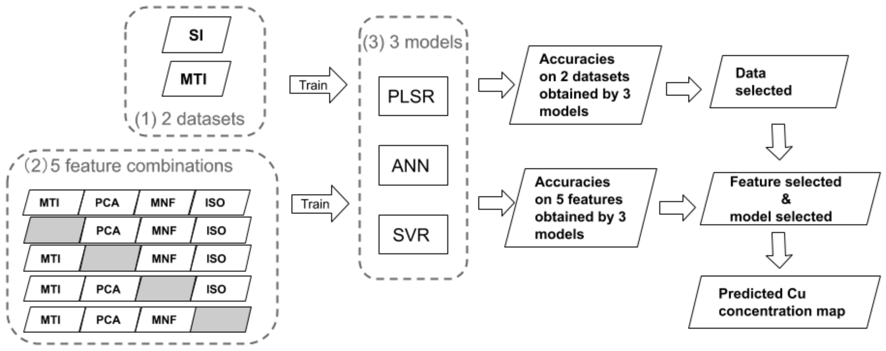
We design an experiment to retrieve soil Cu concentration accurately and effectively by exploring key issues in empirical data inversion, i.e., data preparation, feature extraction and model selection. We compare three regressors that estimate the soil Cu concentration based on four features generated from eleven multi-temporal Landsat-8 images. We employ the cross-validation technique for bias-reduced accuracy measures. The Cu concentration map is generated using the preferred model with its preferred input features. Figure 1 shows the workflow.
3.1. Study Area and Soil Samples
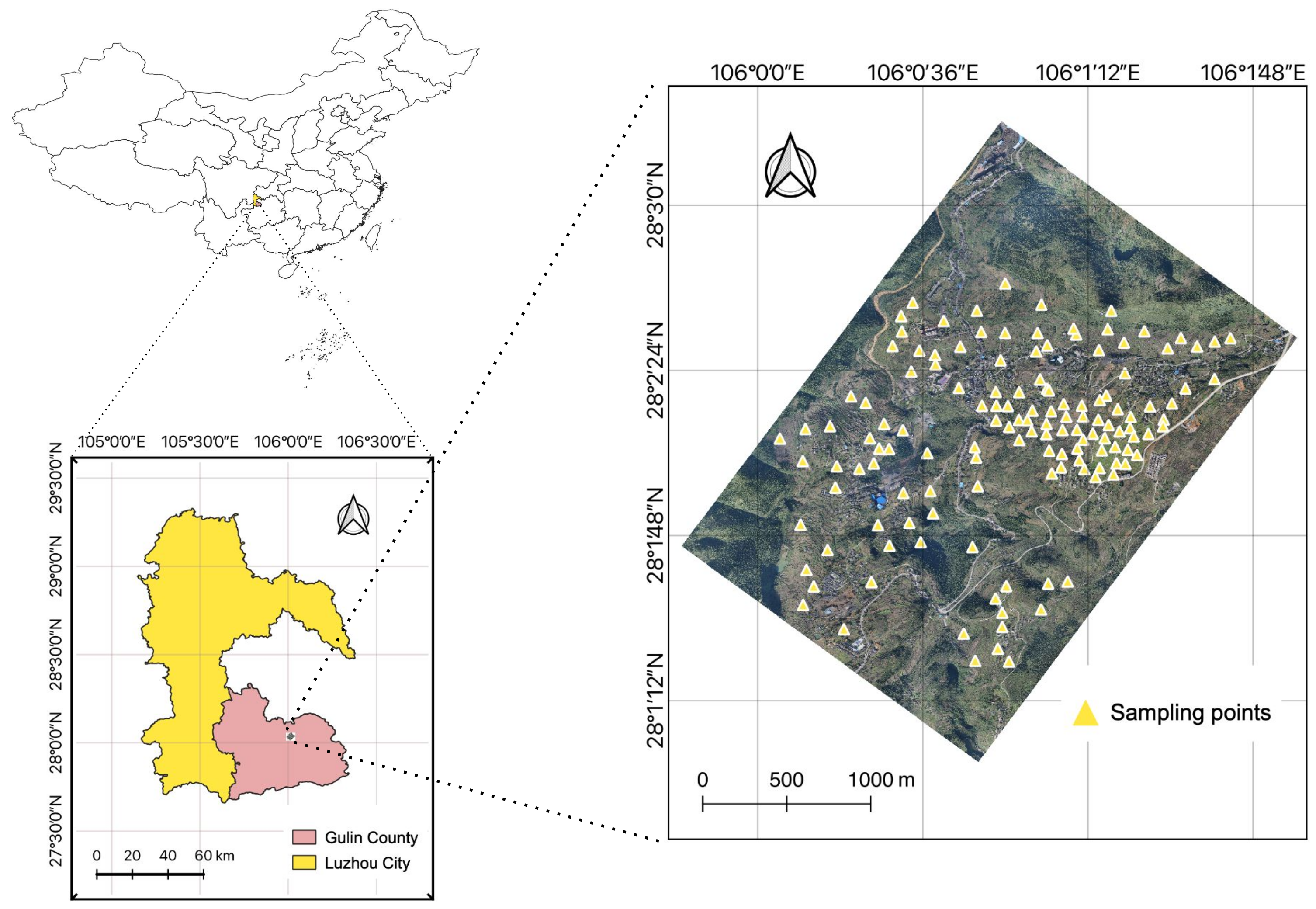
The study area is located in Shiping village, Gulin County, Sichuan Province, China. The area has a subtropical climate, with annual average rainfall 748.4–1184.2 mm [38]. Due to many mining and industrial areas, the area is known to contain heavy metal contamination. The location of the study area and the 3D representation of the remote sensing image are shown in Figure 2. The soil in this area is mainly comprised of mollic gleysols, gleyic luvisols, planosols and eutric fluvisols according to the soil map databased provided by the Food and Agriculture Organization of the United Nations. A total of 138 soil samples were collected in this study area in 2015, and the Cu concentrations of samples were analyzed and recorded.
3.2. Multi-Temporal Images of Landsat-8
In this paper, 11 single date images of Landsat-8 ranging from 2013 to 2017 (path 128, row 40 and 41) are obtained from Geospatial Data Cloud website [39] and selected as the multi-temporal images with the cloudiness coverage lower than . The imagery acquisition dates are summarized in Table 1. The downloaded images are level 1T products after topographic correction and have a 30 m spatial resolution except for the panchromatic band (band 8) with a spatial resolution of 15 m, which is not used in this study. Bands 10 and 11 of the 28 December 2014 imagery were destroyed due to a broken file and had to be excluded. As a result, the combined MTI comprises 108 bands in total.
3.3. Feature Selection
3.3.1. Feature Extraction
Feature extraction projects variables in the original space into a new feature space with a lower dimensionality, finding more meaningful information to improve the model learning performance and build better generalizable models [27]. In this study, three representative feature extraction methods are employed for extracting features from multi-temporal images of Landsat-8. Principal component analysis (PCA), minimum noise fraction (MNF) and isometric feature mapping (ISOMAP) are applied for feature extraction from multi-temporal images. The obtained features extracted by these three methods have 5, 5 and 10 dimensions separately.
3.3.2. Feature Importance Measure
The permutation feature importance measure used to evaluate different groups of features. The rationale is that when a variable is permuted, the connection between this variable and the response is lost. If this variable is associated with the response, using the permuted variable and the remaining unpermuted variables for prediction would lead to the prediction accuracy decreasing. Therefore, by calculating the difference in the prediction accuracy before and after permuting a variable, the importance of this variable can be quantified [40,41].
We explore the importance of four groups of features, i.e., original bands (OB) of MTIs, PCA, MNF and ISOMAP, by removing one of them each time and calculating the difference value of prediction accuracy before and after removing this group of features. In this manner, we can obtain the importance of each group of features related to different models used for predicting different kinds of HMC. Then, we select the “best” feature combination using forward feature selection [42], where the feature groups are added one by one from the most important to the least important until the prediction accuracy not increasing any more.
3.4. Regression Methods
Three regression methods are compared for the retrieval soil Cu concentration from Landsat-8 images. PLSR, ANN and SVM are all popular and efficient regression methods that are commonly used in soil property studies [8,18,43]. PLSR is based on the linear model, ANN represents the data-driven machine learning method and SVR implements regression by building a decision boundary.
3.4.1. Partial Least Square Regression, PLSR
PLSR is a specific form of multivariate linear regression [10], which has been widely used for soil property estimation [22,44,45]. PLSR assumes that the dependent variable can be estimated via a linear combination of explanatory variables [10]. By using the partial least-squares approach, PLSR obtains the projections of both dependent variables and explanatory variables, maximizing the covariance between projections, and then establishes the regression model based on these projections [46]. PLSR has the advantages of effectively dealing with collinear and noisy independent variables, modelling multiple response variables simultaneously [44,47] and having the inferential capability for possible linear relationships [44].
3.4.2. Artificial Neural Network, ANN
ANNs have become a popular machine learning regression algorithm over the last decade [46]. Compared to the linear regression models, ANNs can fit the data and model the complicated underlying relationships more flexibly [48]. Though ANN is good at processing nonlinear and complex problems, even with the inaccurate and noisy data [49], its performance highly relies on the network structure with a proper number of layers and neurons [46].
We use a multiple-layer feed-forward backpropagation network with three layers, including an input layer, a hidden layer and an output layer, with a learning rule based on the Levenberg–Marquardt algorithm. This common structure was adopted in related studies [44,50,51] and turned out to be effective for soil property retrieval. Tan-sigmoid and linear activation functions are applied to the hidden layer and the output layer separately in this study. A common hyperparameter optimization method, grid search [52], is adopted to find the optimal neuron number of the hidden layer in the set of .
3.4.3. Support Vector Regression, SVR
SVR is based on the same principles as the support vector machine for classification by minimizing error and individualizing the hyperplane, which maximizes the margin. As a kernel-based regression method, SVR solves nonlinear regression problems by transferring the data from the original space to a higher dimensional space via a kernel function [53]. In -SVR, the goal is to find an estimation function as flat as possible that has a deviation under from the targets of the training data [54]. In this study, -SVR with a radial basis kernel is adopted to build the HMC inverse model from Landsat-8 imagery. The performance of SVR deeply depends on the hyperparameters [55]. There are two main hyperparameters to set, i.e., cost and . The cost is the penalty associated with errors larger than , and represents the minimally required precision. Optimal hyperparameters are set by performing the grid search in a discretized two-dimensional parameter space.
3.5. Accuracy Measure
To quantify model performances based on different regression methods and different input features, four parameters, including the adjusted coefficient of determination (R), root mean square error (RMSE), mean absolute error (MAE) and standard error (SE), are calculated. R indicates the goodness of fit of the model, ranging from 0 to 1. RMSE indicates the absolute estimation errors [44]. The total MAE is attributed by each error in proportion to its magnitude rather than its square [56]. SE is calculated by taking the standard deviation and dividing it by the square root of the sample size.
3.6. Cross-Validation Estimation
To guarantee an unbiased evaluation of models, the test dataset should be separated from the training dataset and follow the same distribution as the training set [57]. The accuracy measures evaluated should be based on both the training set and the test set to avoid overestimating the generalization ability of complex models due to the overfitting effect [41]. In the k-fold cross-validation, samples are randomly partitioned to k equal-sized subsets, and only one subset is used as the test set. The process is repeated k times so that each of the subsets is used as a test set once. In this study, 6-fold cross-validation is used for model evaluation. Therefore, given 138 soil samples, 115 samples are used to train the model and the remaining 23 samples are used to evaluate the model performance on the test dataset. This is repeated 6 times. In order to obtain results independent of a particular partitioning, this procedure is repeated 20 times, and then models are obtained. Both training and test accuracies of each model are calculated.
For training each model, 5-fold cross-validation is adopted to set hyperparamters that guarantee the best performance of each method, including the number of principal components for PLSR, cost and value for SVR, as well as neuron numbers and learning rate for ANN. Hyperparameters that generate the highest R on test data would be selected for model training.
4. Results
4.1. Comparison between Single and Multi-Temporal Images of Landsat-8
Both the combined MTIs and SIs of Landsat-8 are used to train the regressors (i.e., PLSR, ANN and SVR) for the prediction of the soil Cu concentration. The 20 repeated 6-fold cross-validation is adopted to evaluate the performance of each model using all indicators: R, RMSE, MAE and SE. The mean value of R, as well as the standard deviation of R, are shown in Table 2. The mean values of R on MTIs are higher than that on SI for all regressors, and the standard deviation of R decreases when using MTIs rather than SIs. For MAE and SE, the mean values of MTI are lower than those on SI, and the standard deviation is slightly higher than SI. The mean values of RMSE of PLSR and SVR do not show an obvious advantage of MTIs, given that the mean values increase when using MTIs. For ANN, RMSE reaches a lower RMSE mean and a lower standard deviation.
4.2. Feature Evaluation and Selection
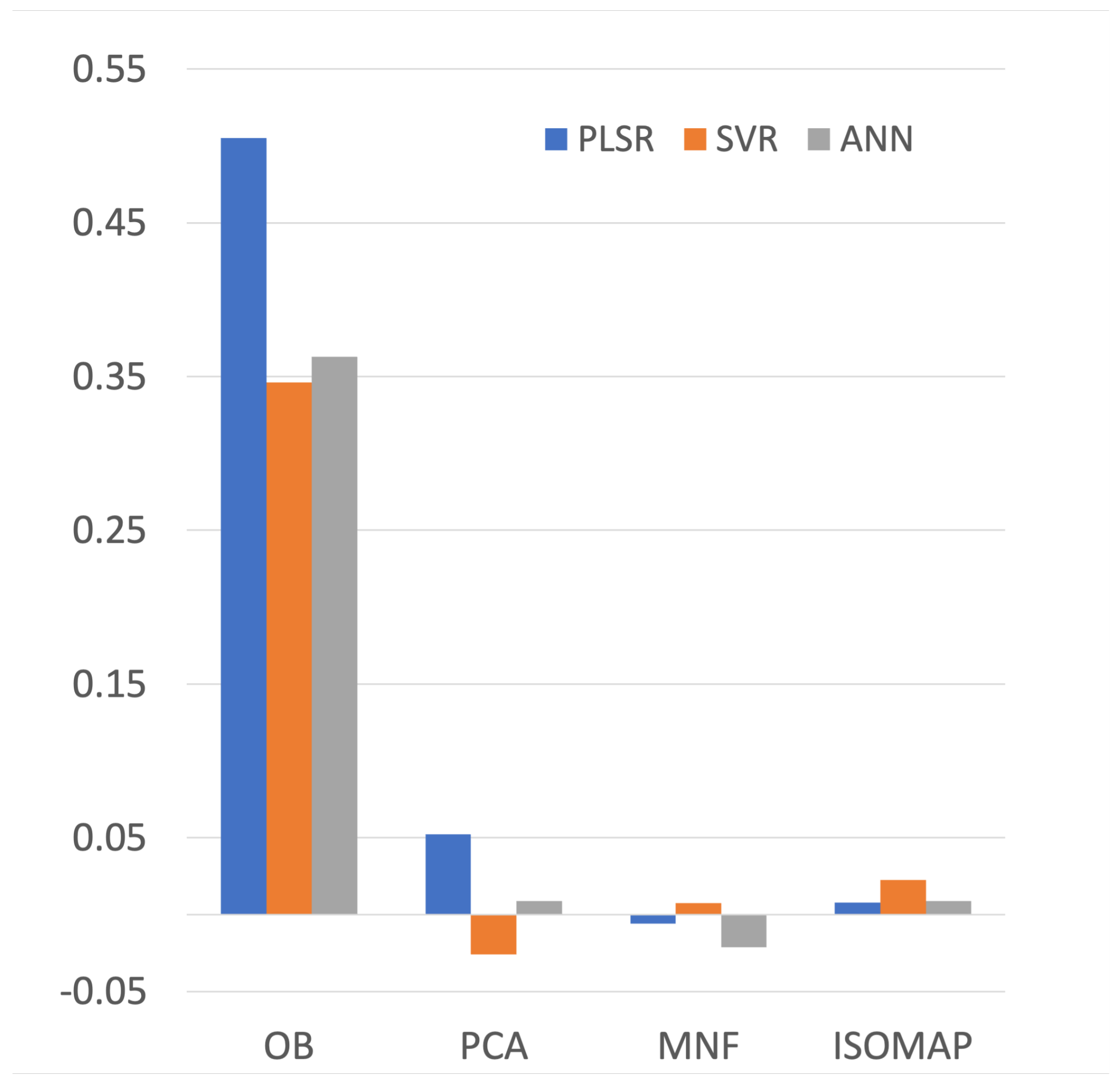
Following the method of feature importance measurement introduced in Section 3.3.2, we first combine all the features to C1 and drop PCA, MNF and ISOMAP one by one to form C2, C3, C4 and C5 separately. The prediction accuracy of these five feature combinations on PLSR, SVR and ANN are summarized in Table 3. By subtracting the adjusted R mean values of C2, C3, C4 and C5 from that of C1 separately, we obtain the feature importance of each feature group, which is plotted in Figure 3. The importance score of these features based on RMSE, MAE and SE are all calculated in addition to the importance score based on R. Except for the RMSE-based importance order of features, other indicators demonstrate the same importance rank. For all three regressors, OB is always the most important feature group for the retrieval of Cu concentration. PCA is the second important feature group for both PLSR and ANN, while SVR takes PCA as the worst input feature. The importance orders of three regressors are listed in Table 4.
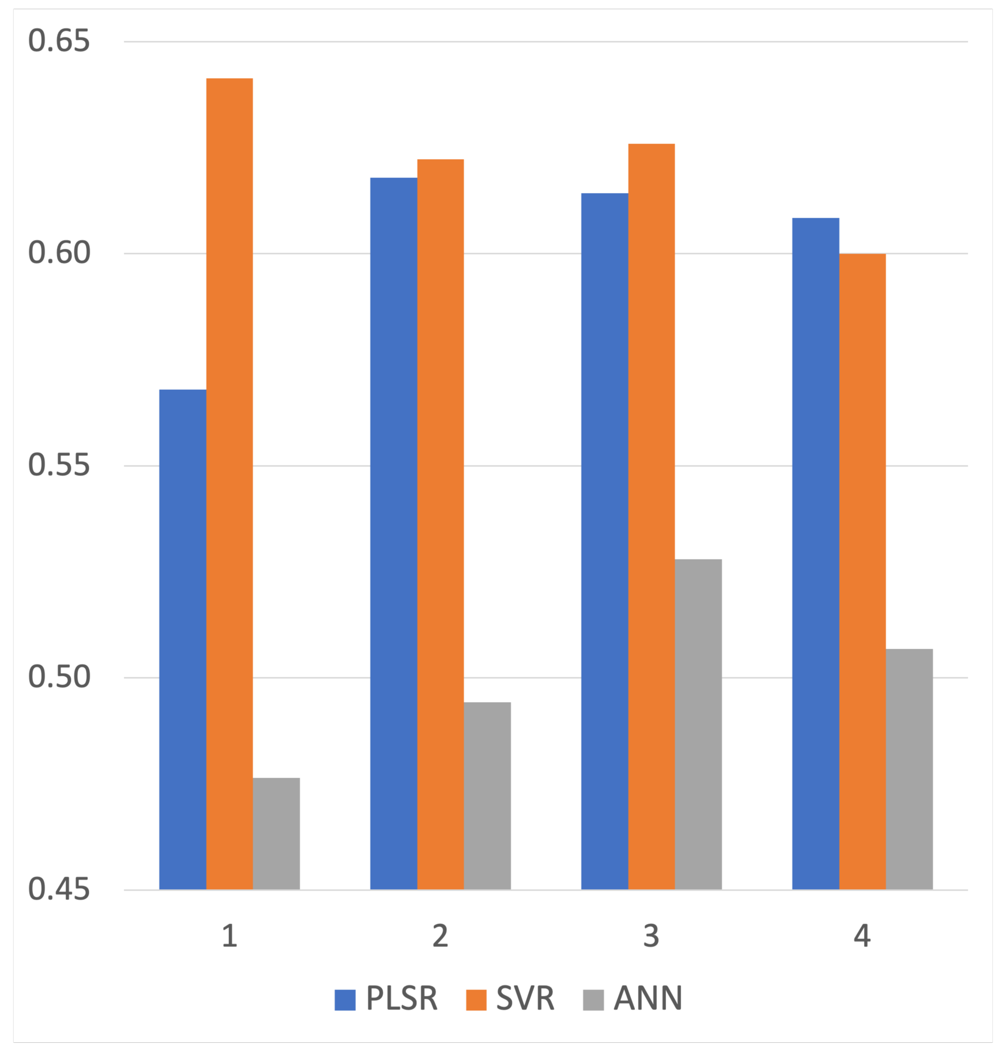
Once the importance order of feature groups for each regressor was obtained, we use the forward feature selection strategy to determine the best feature combination by adding a feature once from the most important to the least important to the model input. For example, for PLSR, we use the OB as the input to train a regressor and test its accuracy. Next, OB together with the second important feature, PCA, is used, then ISOMAP and MNF are added one by one. For all three regressors, we tested the Cu prediction accuracy on different numbers of the feature. The mean values of test R are plotted in Figure 4.
For PLSR and ANN, the overall trend is that R increases first and then decreases as the feature number increases. For SVR, the R has reached the highest value when using OB only and then goes down with the increasing number of features. By identifying the peak positions of three regressors, the best feature combination for each regressor is identified.
4.3. Model Selection
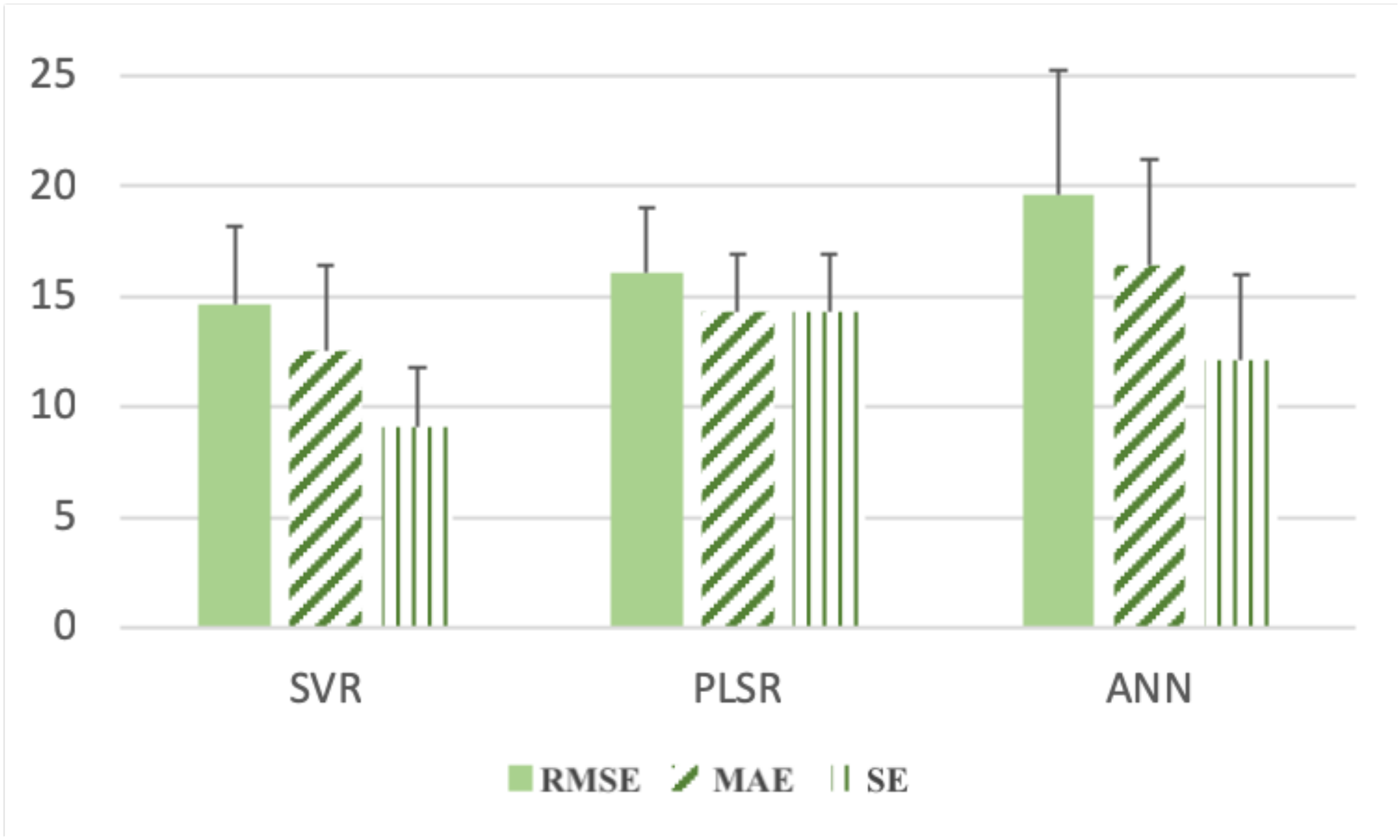
To fairly compare three regressors—PLSR, SVR and ANN—we choose the most preferred feature combination for each regressor to ensure that we are comparing the best performances of these three regressors. We use OB as the input for SVR training, the combination of OB and PCA for PLSR and the combination of OB, PCA and ISOMAP for ANN. Moreover, the hyperparameters of the three models are determined by the grid search approach. Then, the prediction accuracies of three regressors are plotted in Figure 5, including the mean and standard deviation values of RMSE, MAE and ANN, since the R statistics have been displayed in Figure 4. SVR obtains the lowest mean values of RMSE, MAE and SE. PLSR performs worse than SVR and better than ANN.
4.4. Soil Cu Concentration Mapping
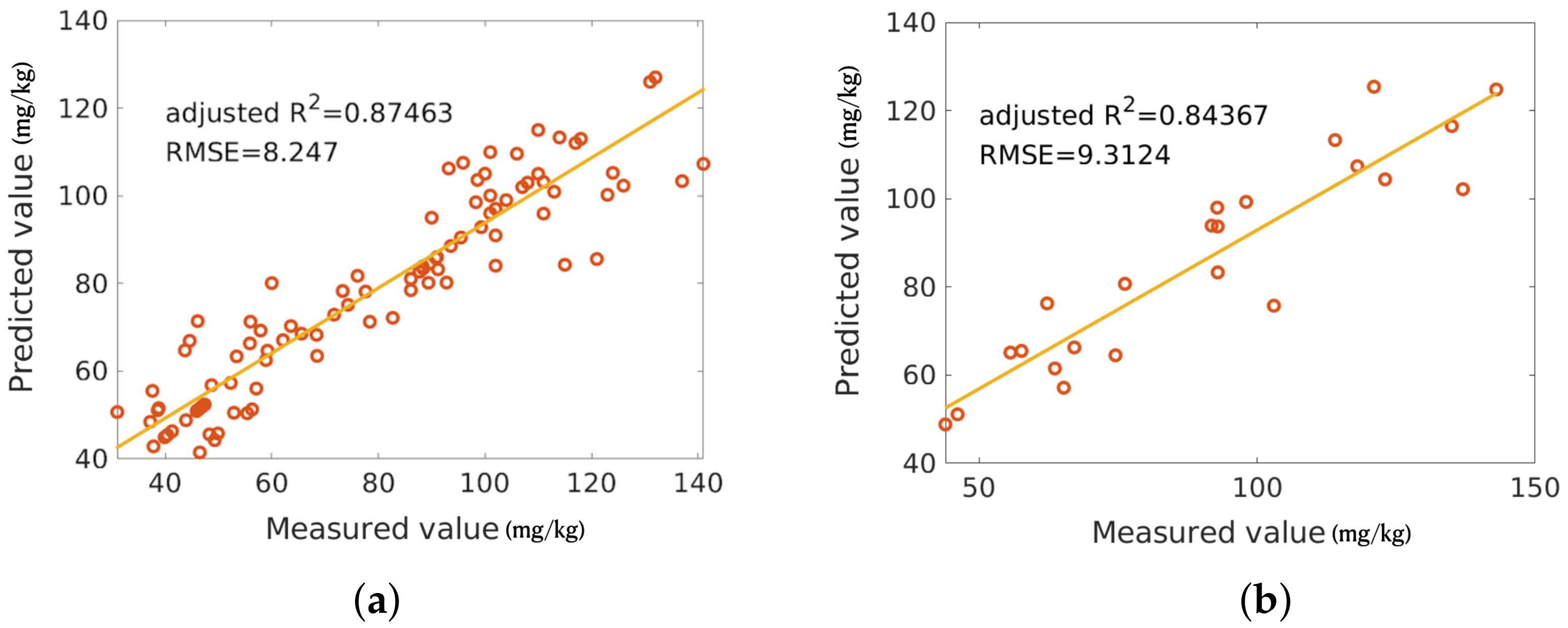
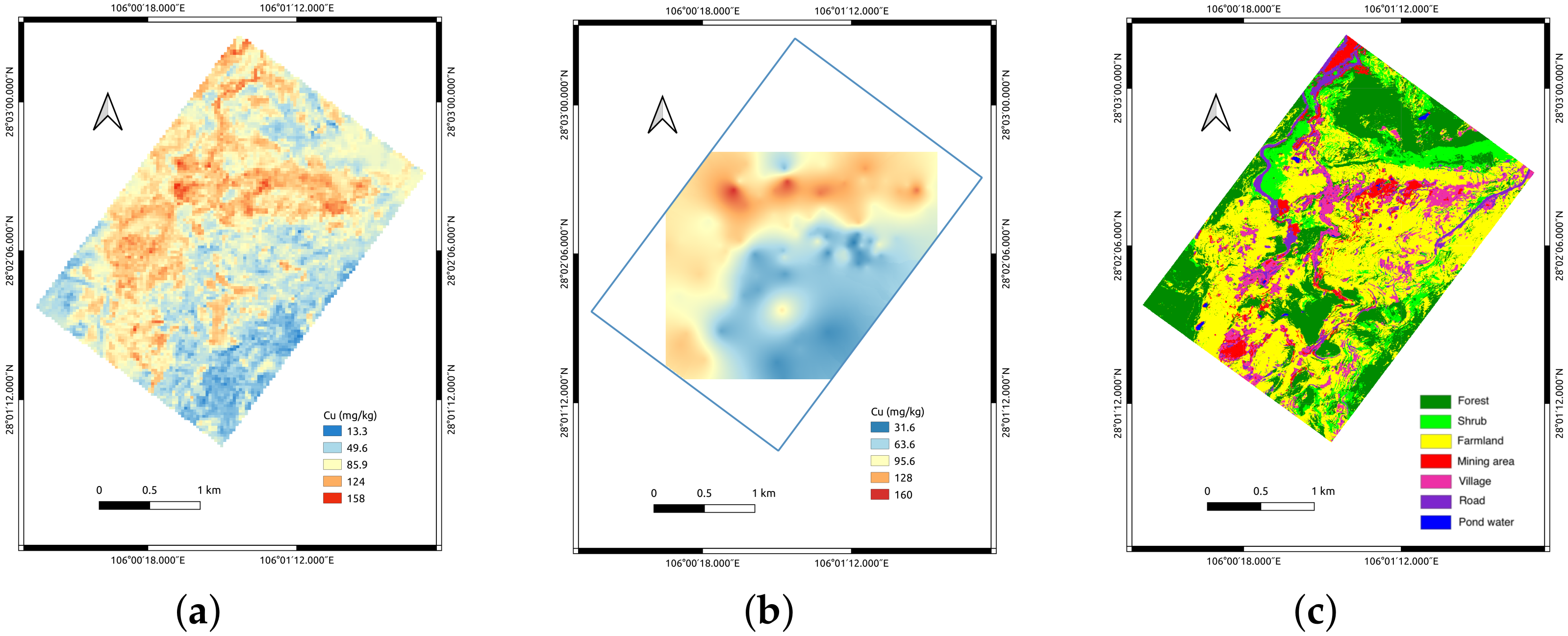
Given the operations of data preparation, feature extraction and model comparison, the OB feature is selected to input into the trained SVR model with the highest prediction R, which is the “best” model among 120 models obtained during the 20 repeated 6-fold cross-validations. The adjusted R of this model reaches 0.87 on the training set and 0.84 on the test set (see Figure 6). By inputting the OB of the images over the entire study area to the preferred SVR model, the Cu concentration distribution map is generated, which is shown in Figure 7a.
To compare the retrieval and mapping of the Cu concentration to the traditional mapping approach based on interpolation, an interpolation map, shown in Figure 7b, is produced using exponential-kriging interpolation [58] on the ArcGIS platform. The exponential semi-variogram model is used as the semi-variance function, where the parameters, including the range, sill and nugget, are default values calculated internally. We set the number of points to 60 within the default search radius. Figure 7a shows more details about the Cu concentration distribution and has a larger spatial coverage compared with Figure 7b.
5. Discussion
5.1. Benefits of Using Multi-Temporal Landsat-8 Images
The experiment results of the comparison between MTIs and SIs (see Section 4.1) show that using MTIs to establish the inversion model of Cu concentration achieves better prediction precision, which is consistent with our assumption that MTIs can enhance the spectral information for a better estimation of Cu concentration. MTI techniques have been adopted to many other applications, e.g., crop classification [59,60] and spectral unmixing [24]. MTIs turned out to be more efficient for classification [59,60], unmixing [24] and land surface property retrieval [25,26] by many studies. Previouse research took advantage of the temporal correlation effect among the MTI observations. For example, for crop type identification, the assumption is that the crop type dictates the temporal patterns in the MTI data, i.e., different crop types tend to have different temporal behaviours. Similarly, we assume the Cu concentration in 2015 is correlated with the MTI observations from the year 2013 to the year 2017, which also generates better inversion accuracy than just using SI.
5.2. Feature Selection
Feature selection is conducted by first ranking four feature groups according to the permutation feature importance and then choosing the useful feature groups via the forward feature selection. As shown in Table 4, all three regressors take OB as the most valuable feature, given that without OB ranking first for all regressors, the estimation accuracy generated by the combination of other remaining features largely decreases. We attribute this importance of OB to its rich spectral information, which can be regarded as multiple repeated observations of the study area. Except for OB, the ranking the feature importance varies with different regressors, which is ascribed to different feature preferences of regressors. For example, PCA is the second most important feature group for both PLSR and ANN but is the least important for SVR (see Figure 3). A related work [41] reports the difference in feature preference between different classifiers on classification tasks.
This paper evaluates one feature importance under the existence of all other features. The importance of a certain feature to a regressor cannot be defined independently without taking into account other input features because its importance can vary with different feature combinations that input into the regressor with this feature. For example, the PCA feature group per se is very helpful for SVR but is less valuable with the existence of OB, MNF and ISOMAP. On the contrary, a feature can be more useful when with other features than itself [42].
5.3. Regressor Comparison
Based on four indicators obtained with the 20 repeated 6-fold cross-validations, SVR turns out to be the model with the best capability of generalization, given that the mean R of prediction is 0.641 and the maximum R of prediction is 0.844, as well as the smallest RMSE, MAE and SE among three regressors. PLSR also performs well with the mean prediction R 0.618 and much better than ANN with the mean prediction R 0.528. Generally speaking, SVR outperforms PLSR, and PLSR outperforms ANN at any feature group number (see Figure 4). In a related study [51], Cu estimation by ANN is also inferior to multiple linear regression. SVR has been demonstrated to have a stronger generalization ability compared to ANN [61,62]. We are not indicating that ANN has no potential capability for soil HMC because not many different architectures with dense grid search for hyperparameters are tested exhaustively. Some research demonstrated that ANN performed well on soil property estimation [18,44]. Particularly for the HMC retrieval from Landsat images, ANN outperforms PLSR, and the R exceeds 0.8 for the concentration estimation of As, Cd, Ni and Pb [50]. This inconsistency in ANN performance between this work and other works is attributed to the different heavy metal categories, study area, training samples, network structures and hyperparameters, which need further study.
5.4. Cu Concentration Mapping
To evaluate the Cu concentration map, the classification map of this study area is introduced, which is provided by China Land Consolidation and Rehabilitation. The red regions on the classification map (Figure 7c) represent the mining area, the positions of which are consistent with the distribution of red areas representing a high Cu concentration in the Cu distribution map (Figure 7a). In the areas of farmland and forest (yellow and green on the classification map), the Cu concentration is much lower (blue areas of Figure 7a). The Cu concentration map can be explained by the classification map by assuming that Cu contamination is caused by the mining activities of humans.
Comparing the obtained Cu concentration map using the proposed pipeline with the interpolation Cu concentration map, it is observed that the distributions of Cu in these two maps share a similar distribution pattern with different spatial coverages and resolutions. Figure 7a is mapped based on pixels, and Figure 7b is produced based on sample points, so Figure 7a contains more spatial details. Another advantage of the proposed method is that the trained model has better extrapolation abilities, while the prediction area of Figure 7b is limited due to the poor extrapolation capability of interpolation methods.
5.5. Uncertainty Analysis
Although the proposed data processing pipeline leads to fairly accurate soil Cu concentration estimation, there is still a discrepancy between the estimated values and the true values of the Cu concentration, which could be caused by uncertainties in both (i) feature extraction and regression models and (ii) data.
The model uncertainty is fundamentally caused by the lack of knowledge about the true relationship between Cu concentration and remote sensing observations. In this paper, an empirical approach consisting of feature extraction and regression models is used to approximate this true relationship. Nevertheless, this approximation will inevitably lead to model bias, especially if the feature extraction and regression models are not optimized. Previous research indicates that feature selection and model selection can produce better prediction accuracy [28,29,38], where cross-validation and bootstrapping approaches are used to better utilize limited training samples [30,37,63,64]. Although this paper tries to reduce this model bias by comparing and identifying the “best” feature extraction and regression approaches and the “best” data processing pipeline, there might still be remaining model bias due to limitations of our research. For example, this study is still limited due to the limited number of feature extraction approaches and regression methods, as well as the coarse grid search density. Furthermore, for model evaluation matrices, only some classical matrices are used in this paper. However, using more matrices, e.g., residual prediction deviation or the ratio of performance to interquartile distance, might help to evaluate models more comprehensively, which could be considered for future work.
The data uncertainty is essentially caused by the inexactness, incompleteness, and insufficiency of the training samples. For example, the spatial distribution and quantity of soil samples might not be able to well-characterize the heterogeneity of the study area. The samples are not uniformly distributed in all land use types due to access limitation. The samples from the forestland are few, which could easily lead to bias for the Cu estimation over the forestland. Furthermore, although the Cu concentration of soil samples are collected and measured by a professional institution, there might be inaccuracy and even errors in the provided results.
6. Conclusions
This paper has proposed a pipeline for retrieving and mapping soil Cu concentration from Landsat MTIs. First, repeated satellite observations were utilized to enhance the spectral information of images. Second, the preferred feature is extracted and selected by systematically evaluating the feature importance. Third, the preferred model is selected by the bias-reduced model evaluation.
MTI was demonstrated to be able to make a more reliable and accurate estimation of Cu concentration using empirical regression methods. By utilizing 11 images of Landsat-8 captured in different time phases, the mean adjusted R obtained by SVR using 20 repeated 6-fold cross-validations on 138 soil samples increases from 0.433 to 0.641. Based on the OB of the MTIs, feature extraction and selection further facilitate the improvement of Cu concentration estimation. The mean R of PLSR and ANN increase from 0.568 to 0.618 and from 0.476 to 0.528 separately, indicating the necessity and benefit of feature extraction and selection. Using cross-validation estimation, PLSR, SVR and ANN are compared unbiasedly based on their best performances using their favourite feature combinations. Although ANN is a popular regression method, in our work, SVR outperforms ANN by achieving a mean R of 0.641, which is 21.4% higher than ANN. RMSE, MAE and SE also support the highest generalization capability of SVR.
The preferred model with the highest R obtained by SVR is selected to estimate the Cu concentration in soil over the study area. Compared to the interpolation map, the Cu concentration distribution map generated by the recommended pipeline gives the pixel-based Cu estimation with more spatial detail and wider spatial coverage. It also shows a consistent spatial pattern with the ground-truth land cover classification map. The results show this model’s ability to perform large-scale soil HMC mapping from widely avaliable satellite imagery.
Author Contributions
Y.F. performed the data collection, data processing, methodology and experiments.; conceptualization, Y.F. and L.X.; writing—original draft preparation, Y.F.; writing—review and editing, L.X., D.A.C. and A.W.; visualization, Y.F.; supervision, L.X. and D.A.C. All authors have read and agreed to the published version of the manuscript.
Funding
This research was funded in part by the Natural Sciences and Engineering Research Council of Canada (NSERC) under Grant RGPIN-2017-04869, Grant DGDND-2017-00078, Grant RGPAS2017-50794 and Grant RGPIN-2019-06744.
Institutional Review Board Statement
Not applicable.
Informed Consent Statement
Not applicable.
Data Availability Statement
The data presented in this study are available on request from the corresponding author.
Conflicts of Interest
The authors declare no conflict of interest.
Sample Availability
Samples of the compounds are available from the authors.
References
- Wild, A. Soils and the Environment; Cambridge University Press: Cambridge, UK, 1993. [Google Scholar]
- Alloway, B.J. Heavy Metals in Soils: Trace Metals and Metalloids in Soils and Their Bioavailability; Springer Science & Business Media: New York, NY, USA, 2012; Volume 22. [Google Scholar]
- McBratney, A.B.; Odeh, I.O.; Bishop, T.F.; Dunbar, M.S.; Shatar, T.M. An overview of pedometric techniques for use in soil survey. Geoderma 2000, 97, 293–327. [Google Scholar] [CrossRef]
- Slonecker, T.; Fisher, G.B.; Aiello, D.P.; Haack, B. Visible and infrared remote imaging of hazardous waste: A review. Remote Sens. 2010, 2, 2474–2508. [Google Scholar] [CrossRef] [Green Version]
- Choe, E.; Kim, K.W.; Bang, S.; Yoon, I.H.; Lee, K.Y. Qualitative analysis and mapping of heavy metals in an abandoned Au-Ag mine area using NIR spectroscopy. Environ. Geol. 2009, 58, 477–482. [Google Scholar] [CrossRef]
- JiA, J.; Song, Y.; Yuan, X.; Yang, Z. Diffuse reflectance spectroscopy study of heavy metals in agricultural soils of the Changjiang River Delta, China. In Proceedings of the 19th World Congress of Soil Science, Brisbane, Australia, 1–6 August 2010. [Google Scholar]
- Choe, E.; van der Meer, F.; van Ruitenbeek, F.; van der Werff, H.; de Smeth, B.; Kim, K.W. Mapping of heavy metal pollution in stream sediments using combined geochemistry, field spectroscopy, and hyperspectral remote sensing: A case study of the Rodalquilar mining area, SE Spain. Remote Sens. Environ. 2008, 112, 3222–3233. [Google Scholar] [CrossRef]
- Maliki, A.A.; Bruce, D.; Owens, G. Capabilities of remote sensing hyperspectral images for the detection of lead contamination: A review. In Proceedings of the ISPRS Annals of the Photogrammetry, Remote Sensing and Spatial Information Sciences, Melbourne, Australia, 25 August–1 September 2012; Volume 55. [Google Scholar]
- Liu, Y.; Li, W.; Wu, G.; Xu, X. Feasibility of estimating heavy metal contaminations in floodplain soils using laboratory-based hyperspectral data—A case study along Le’an River, China. Geo-Spat. Inf. Sci. 2011, 14, 10–16. [Google Scholar] [CrossRef] [Green Version]
- Wang, F.; Gao, J.; Zha, Y. Hyperspectral sensing of heavy metals in soil and vegetation: Feasibility and challenges. ISPRS J. Photogramm. Remote Sens. 2018, 136, 73–84. [Google Scholar] [CrossRef]
- Hong-Yan, R.; Zhuang, D.F.; Singh, A.; Jian-Jun, P.; Dong-Sheng, Q.; Run-He, S. Estimation of As and Cu contamination in agricultural soils around a mining area by reflectance spectroscopy: A case study. Pedosphere 2009, 19, 719–726. [Google Scholar]
- Zhang, X.; Huang, C.; Liu, B.; Tong, Q. Inversion of soil Cu concentration based on band selection of hyperspetral data. In Proceedings of the 2010 IEEE International Geoscience and Remote Sensing Symposium, Honolulu, HI, USA, 25–30 July 2010; pp. 3680–3683. [Google Scholar]
- Phiri, D.; Morgenroth, J. Developments in Landsat land cover classification methods: A review. Remote Sens. 2017, 9, 967. [Google Scholar] [CrossRef] [Green Version]
- Kalma, J.D.; McVicar, T.R.; McCabe, M.F. Estimating land surface evaporation: A review of methods using remotely sensed surface temperature data. Surv. Geophys. 2008, 29, 421–469. [Google Scholar] [CrossRef]
- Quattrochi, D.A.; Luvall, J.C. Thermal Remote Sensing in Land Surface Processing; CRC Press: Boca Raton, FL, USA, 2004. [Google Scholar]
- Skakun, S.; Vermote, E.; Roger, J.C.; Franch, B. Combined use of Landsat-8 and Sentinel-2A images for winter crop mapping and winter wheat yield assessment at regional scale. AIMS Geosci. 2017, 3, 163. [Google Scholar] [CrossRef]
- Wallis, C.I.; Homeier, J.; Peña, J.; Brandl, R.; Farwig, N.; Bendix, J. Modeling tropical montane forest biomass, productivity and canopy traits with multispectral remote sensing data. Remote Sens. Environ. 2019, 225, 77–92. [Google Scholar] [CrossRef]
- Ali, A.M.; Darvishzadeh, R.; Skidmore, A.K. Retrieval of specific leaf area from Landsat-8 surface reflectance data using statistical and physical models. IEEE J. Sel. Top. Appl. Earth Obs. Remote Sens. 2017, 10, 3529–3536. [Google Scholar] [CrossRef]
- Middinti, S.; Thumaty, K.C.; Gopalakrishnan, R.; Jha, C.S.; Thatiparthi, B.R. Estimating the leaf area index in Indian tropical forests using Landsat-8 OLI data. Int. J. Remote Sens. 2017, 38, 6769–6789. [Google Scholar] [CrossRef]
- Sadeghi, M.; Babaeian, E.; Tuller, M.; Jones, S.B. The optical trapezoid model: A novel approach to remote sensing of soil moisture applied to Sentinel-2 and Landsat-8 observations. Remote Sens. Environ. 2017, 198, 52–68. [Google Scholar] [CrossRef] [Green Version]
- Amani, M.; Parsian, S.; MirMazloumi, S.M.; Aieneh, O. Two new soil moisture indices based on the NIR-red triangle space of Landsat-8 data. Int. J. Appl. Earth Obs. Geoinf. 2016, 50, 176–186. [Google Scholar] [CrossRef]
- Aldabaa, A.A.A.; Weindorf, D.C.; Chakraborty, S.; Sharma, A.; Li, B. Combination of proximal and remote sensing methods for rapid soil salinity quantification. Geoderma 2015, 239, 34–46. [Google Scholar] [CrossRef] [Green Version]
- Guerschman, J.P.; Paruelo, J.; Bella, C.D.; Giallorenzi, M.; Pacin, F. Land cover classification in the Argentine Pampas using multi-temporal Landsat TM data. Int. J. Remote Sens. 2003, 24, 3381–3402. [Google Scholar] [CrossRef]
- Zurita-Milla, R.; Gómez-Chova, L.; Guanter, L.; Clevers, J.G.; Camps-Valls, G. Multitemporal unmixing of medium-spatial-resolution satellite images: A case study using MERIS images for land-cover mapping. IEEE Trans. Geosci. Remote Sens. 2011, 49, 4308–4317. [Google Scholar] [CrossRef]
- Mattia, F.; Satalino, G.; Pauwels, V.; Alexander, L. Soil moisture retrieval through a merging of multi-temporal L-band SAR data and hydrologic modelling. Hydrol. Earth Syst. Sci. 2009, 13, 343–356. [Google Scholar] [CrossRef] [Green Version]
- Kurvonen, L.; Pulliainen, J.; Hallikainen, M. Retrieval of biomass in boreal forests from multitemporal ERS-1 and JERS-1 SAR images. IEEE Trans. Geosci. Remote Sens. 1999, 37, 198–205. [Google Scholar] [CrossRef] [Green Version]
- Tang, J.; Alelyani, S.; Liu, H. Feature selection for classification: A review. In Data Classification: Algorithms and Applications; CRC Press: Boca Raton, FL, USA, 2014; p. 37. [Google Scholar]
- Xiaobo, Z.; Jiewen, Z.; Povey, M.J.; Holmes, M.; Hanpin, M. Variables selection methods in near-infrared spectroscopy. Anal. Chim. Acta 2010, 667, 14–32. [Google Scholar] [CrossRef]
- Balabin, R.M.; Smirnov, S.V. Variable selection in near-infrared spectroscopy: Benchmarking of feature selection methods on biodiesel data. Anal. Chim. Acta 2011, 692, 63–72. [Google Scholar] [CrossRef]
- Wang, J.; Shi, T.; Yu, D.; Teng, D.; Ge, X.; Zhang, Z.; Yang, X.; Wang, H.; Wu, G. Ensemble machine-learning-based framework for estimating total nitrogen concentration in water using drone-borne hyperspectral imagery of emergent plants: A case study in an arid oasis, NW China. Environ. Pollut. 2020, 266, 115412. [Google Scholar] [CrossRef]
- Wang, J.; Hu, X.; Shi, T.; He, L.; Hu, W.; Wu, G. Assessing toxic metal chromium in the soil in coal mining areas via proximal sensing: Prerequisites for land rehabilitation and sustainable development. Geoderma 2022, 405, 115399. [Google Scholar] [CrossRef]
- Wu, Y.; Chen, J.; Wu, X.; Tian, Q.; Ji, J.; Qin, Z. Possibilities of reflectance spectroscopy for the assessment of contaminant elements in suburban soils. Appl. Geochem. 2005, 20, 1051–1059. [Google Scholar] [CrossRef]
- Pinheiro, É.; Ceddia, M.; Clingensmith, C.; Grunwald, S.; Vasques, G. Prediction of soil physical and chemical properties by visible and near-infrared diffuse reflectance spectroscopy in the central Amazon. Remote Sens. 2017, 9, 293. [Google Scholar] [CrossRef] [Green Version]
- Zhao, Y.; Li, X.; Yu, K.; Cheng, F.; He, Y. Hyperspectral Imaging for Determining Pigment Contents in Cucumber Leaves in Response to Angular Leaf Spot Disease. Sci. Rep. 2016, 6, 27790. [Google Scholar] [CrossRef] [PubMed]
- Li, F.; Mistele, B.; Hu, Y.; Chen, X.; Schmidhalter, U. Reflectance estimation of canopy nitrogen content in winter wheat using optimised hyperspectral spectral indices and partial least squares regression. Eur. J. Agron. 2014, 52, 198–209. [Google Scholar] [CrossRef]
- Di, W.U.; Nie, P.; Joel, C.; Yong, H.E.; Wang, Z.; Hongxi, W.U. Application of visible and near infrared spectroscopy for rapid and non-invasive quantification of common adulterants in Spirulina powder. J. Food Eng. 2011, 102, 278–286. [Google Scholar]
- Wei, C.; Huang, J.; Wang, X.; Blackburn, G.A.; Zhang, Y.; Wang, S.; Mansaray, L.R. Hyperspectral characterization of freezing injury and its biochemical impacts in oilseed rape leaves. Remote Sens. Environ. 2017, 195, 56–66. [Google Scholar] [CrossRef] [Green Version]
- Fang, Y.; Xu, L.; Peng, J.; Wang, H.; Wong, A.; Clausi, D.A. Retrieval and mapping of heavy metal concentration in soil using time seies Landsat 8 imagery. In Proceedings of the International Archives of the Photogrammetry, Remote Sensing & Spatial Information Sciences, Beijing, China, 7–10 May 2018; Volume 42. [Google Scholar]
- Geospatial Data Cloud. Available online: http://www.gscloud.cn/ (accessed on 8 April 2018).
- Strobl, C.; Boulesteix, A.L.; Zeileis, A.; Hothorn, T. Bias in random forest variable importance measures: Illustrations, sources and a solution. BMC Bioinform. 2007, 8, 25. [Google Scholar] [CrossRef] [Green Version]
- Xu, L.; Li, J.; Brenning, A. A comparative study of different classification techniques for marine oil spill identification using RADARSAT-1 imagery. Remote Sens. Environ. 2014, 141, 14–23. [Google Scholar] [CrossRef]
- Guyon, I.; Elisseeff, A. An introduction to variable and feature selection. J. Mach. Learn. Res. 2003, 3, 1157–1182. [Google Scholar]
- Minu, S.; Shetty, A.; Gopal, B. Review of preprocessing techniques used in soil property prediction from hyperspectral data. Cogent Geosci. 2016, 2, 1145878. [Google Scholar] [CrossRef]
- Farifteh, J.; Van der Meer, F.; Atzberger, C.; Carranza, E. Quantitative analysis of salt-affected soil reflectance spectra: A comparison of two adaptive methods (PLSR and ANN). Remote Sens. Environ. 2007, 110, 59–78. [Google Scholar] [CrossRef]
- Yu, H.; Liu, M.; Du, B.; Wang, Z.; Hu, L.; Zhang, B. Mapping Soil Salinity/Sodicity by using Landsat OLI Imagery and PLSR Algorithm over Semiarid West Jilin Province, China. Sensors 2018, 18, 1048. [Google Scholar] [CrossRef] [Green Version]
- Verrelst, J.; Camps-Valls, G.; Muñoz-Marí, J.; Rivera, J.P.; Veroustraete, F.; Clevers, J.G.; Moreno, J. Optical remote sensing and the retrieval of terrestrial vegetation bio-geophysical properties—A review. ISPRS J. Photogramm. Remote Sens. 2015, 108, 273–290. [Google Scholar] [CrossRef]
- Wold, S.; Sjöström, M.; Eriksson, L. PLS-regression: A basic tool of chemometrics. Chemom. Intell. Lab. Syst. 2001, 58, 109–130. [Google Scholar] [CrossRef]
- Zhang, G.P. Neural networks for classification: A survey. IEEE Trans. Syst. Man Cybern. Part C (Appl. Rev.) 2000, 30, 451–462. [Google Scholar] [CrossRef] [Green Version]
- Jaroenpoj, S.; Yu, J.; Ness, J. Development of artificial neural network models for biogas production from co-digestion of leachate and pineapple peel. Glob. Environ. Eng. 2015, 1, 42–47. [Google Scholar] [CrossRef] [Green Version]
- Fard, R.S.; Matinfar, H.R. Capability of vis-NIR spectroscopy and Landsat-8 spectral data to predict soil heavy metals in polluted agricultural land (Iran). Arab. J. Geosci. 2016, 9, 745. [Google Scholar] [CrossRef]
- Kemper, T.; Sommer, S. Estimate of heavy metal contamination in soils after a mining accident using reflectance spectroscopy. Environ. Sci. Technol. 2002, 36, 2742–2747. [Google Scholar] [CrossRef]
- LeCun, Y.; Bottou, L.; Bengio, Y.; Haffner, P. Gradient-based learning applied to document recognition. Proc. IEEE 1998, 86, 2278–2324. [Google Scholar] [CrossRef] [Green Version]
- Verrelst, J.; Malenovskỳ, Z.; Van der Tol, C.; Camps-Valls, G.; Gastellu-Etchegorry, J.P.; Lewis, P.; North, P.; Moreno, J. Quantifying vegetation biophysical variables from imaging spectroscopy data: A review on retrieval methods. Surv. Geophys. 2018, 40, 589–629. [Google Scholar] [CrossRef] [Green Version]
- Smola, A.J.; Schölkopf, B. A tutorial on support vector regression. Stat. Comput. 2004, 14, 199–222. [Google Scholar] [CrossRef] [Green Version]
- Karasuyama, M.; Nakano, R. Optimizing SVR hyperparameters via fast cross-validation using AOSVR. In Proceedings of the 2007 International Joint Conference on Neural Networks, Orlando, FL, USA, 12–17 August 2007; pp. 1186–1191. [Google Scholar]
- Willmott, C.J.; Matsuura, K. Advantages of the mean absolute error (MAE) over the root mean square error (RMSE) in assessing average model performance. Clim. Res. 2005, 30, 79–82. [Google Scholar] [CrossRef]
- Hand, D.J. Construction and Assessment of Classification Rules; Wiley: Chichester, UK, 1997; Volume 15. [Google Scholar]
- Childs, C. Interpolating surfaces in ArcGIS spatial analyst. Arcuser 2004, 3235, 569. [Google Scholar]
- Ozdogan, M. The spatial distribution of crop types from MODIS data: Temporal unmixing using Independent Component Analysis. Remote Sens. Environ. 2010, 114, 1190–1204. [Google Scholar] [CrossRef]
- Vuolo, F.; Neuwirth, M.; Immitzer, M.; Atzberger, C.; Ng, W.T. How much does multi-temporal Sentinel-2 data improve crop type classification? Int. J. Appl. Earth Obs. Geoinf. 2018, 72, 122–130. [Google Scholar] [CrossRef]
- Çimen, M.; Kisi, O. Comparison of two different data-driven techniques in modeling lake level fluctuations in Turkey. J. Hydrol. 2009, 378, 253–262. [Google Scholar] [CrossRef]
- Balabin, R.M.; Lomakina, E.I. Support vector machine regression (SVR/LS-SVM)—An alternative to neural networks (ANN) for analytical chemistry? Comparison of nonlinear methods on near infrared (NIR) spectroscopy data. Analyst 2011, 136, 1703–1712. [Google Scholar] [CrossRef]
- Inoue, Y.; Sakaiya, E.; Zhu, Y.; Takahashi, W. Diagnostic mapping of canopy nitrogen content in rice based on hyperspectral measurements. Remote Sens. Environ. 2012, 126, 210–221. [Google Scholar] [CrossRef]
- Shi, T.; Hu, X.; Guo, L.; Su, F.; Tu, W.; Hu, Z.; Liu, H.; Yang, C.; Wang, J.; Zhang, J.; et al. Digital mapping of zinc in urban topsoil using multisource geospatial data and random forest. Sci. Total Environ. 2021, 792, 148455. [Google Scholar] [CrossRef]
Figure 1.
Workflow of the proposed baseline for Cu concentration mapping.

Figure 2.
Location of the study area and the distribution of soil samples.

Figure 3.
Feature importance of OB, PCA, MNF and ISOMAP for PLSR, SVR and ANN.

Figure 4.
The mean values of R on 20 repeated 6-fold cross-validations using a different number of feature groups for Cu estimation.
Figure 4.
The mean values of R on 20 repeated 6-fold cross-validations using a different number of feature groups for Cu estimation.

Figure 5.
The mean value and standard deviation of RMSE, MAE and SE obtained by SVR, PLSR and ANN using 20 repeated 6-fold cross-validations.
Figure 5.
The mean value and standard deviation of RMSE, MAE and SE obtained by SVR, PLSR and ANN using 20 repeated 6-fold cross-validations.

Figure 6.
Scatterplot of the best SVR model for Cu concentration estimation on (a) the training dataset and (b) the test dataset.
Figure 6.
Scatterplot of the best SVR model for Cu concentration estimation on (a) the training dataset and (b) the test dataset.

Figure 7.
Cu concentration mapping and evaluation: (a) the distribution map of Cu concentration generated by trained SVR model; (b) the distribution map of Cu concentration obtained by E-kriging interpolation; (c) the classification map of the study area.
Figure 7.
Cu concentration mapping and evaluation: (a) the distribution map of Cu concentration generated by trained SVR model; (b) the distribution map of Cu concentration obtained by E-kriging interpolation; (c) the classification map of the study area.


Table 1.
Landsat-8 image acquisition dates.
| 2013 | 2014 | 2015 | 2016 | 2017 |
|---|---|---|---|---|
| 16 June 2013 | 6 August 2014 a | 3 April 2015 a | 8 June 2016 | 19 February 2017 |
| 6 August 2014 b | 3 April 2015 b | 26 July 2015 | ||
| 9 October 2014 | 8 July 2015 | |||
| 28 December 2014 |
“a” represents for the image from row 40 of the satellite; “b” represents for the image from row 41 of the satellite.
Table 2.
The mean and standard deviation values of regression indicators on three regressors over 20 repeated 6-fold cross-validation using MTL and SI on the training dataset and the test dataset.
Table 2.
The mean and standard deviation values of regression indicators on three regressors over 20 repeated 6-fold cross-validation using MTL and SI on the training dataset and the test dataset.
| PLSR | SVR | ANN | |||||
|---|---|---|---|---|---|---|---|
| Mean | Std.dev | Mean | Std.dev | Mean | Std.dev | ||
| Adjusted R | MTI | 0.568 | 0.131 | 0.641 | 0.160 | 0.476 | 0.197 |
| SI | 0.368 | 0.148 | 0.433 | 0.237 | 0.249 | 0.185 | |
| RMSE | MTI | 16.997 | 3.178 | 15.515 | 3.426 | 20.651 | 5.664 |
| SI | 16.257 | 3.014 | 14.636 | 3.508 | 23.305 | 6.213 | |
| MAE | MTI | 15.215 | 3.021 | 12.498 | 3.914 | 17.673 | 5.444 |
| SI | 19.493 | 2.752 | 16.711 | 4.857 | 22.994 | 5.310 | |
| SE | MTI | 15.215 | 3.021 | 9.099 | 2.691 | 12.910 | 4.270 |
| SI | 19.493 | 2.752 | 11.874 | 3.915 | 14.504 | 4.461 | |
The highest accuracies are in bold format.
Table 3.
Mean and standard deviation of prediction accuracies of Cu concentration estimated by PLSR, SVR and ANN using 20 repeated 6-fold cross-validations.
Table 3.
Mean and standard deviation of prediction accuracies of Cu concentration estimated by PLSR, SVR and ANN using 20 repeated 6-fold cross-validations.
| PLSR | SVR | ANN | PLSR | SVR | ANN | ||
|---|---|---|---|---|---|---|---|
| Mean | Std.dev. | ||||||
| Adjusted R | C1 | 0.608 | 0.600 | 0.507 | 0.134 | 0.169 | 0.183 |
| C2 | 0.103 | 0.254 | 0.144 | 0.119 | 0.233 | 0.154 | |
| C3 | 0.556 | 0.626 | 0.498 | 0.117 | 0.143 | 0.206 | |
| C4 | 0.614 | 0.593 | 0.528 | 0.109 | 0.164 | 0.186 | |
| C5 | 0.601 | 0.577 | 0.498 | 0.132 | 0.158 | 0.186 | |
| RMSE | C1 | 16.384 | 14.741 | 20.338 | 3.543 | 3.806 | 5.407 |
| C2 | 14.809 | 20.707 | 27.151 | 4.858 | 4.910 | 8.275 | |
| C3 | 17.920 | 15.314 | 20.522 | 4.569 | 3.519 | 6.533 | |
| C4 | 16.365 | 15.335 | 19.598 | 3.571 | 3.385 | 5.628 | |
| C5 | 16.532 | 15.515 | 21.511 | 2.952 | 3.426 | 5.741 | |
| MAE | C1 | 14.475 | 13.698 | 16.717 | 2.955 | 4.140 | 4.722 |
| C2 | 24.426 | 20.835 | 26.282 | 3.854 | 5.491 | 5.900 | |
| C3 | 15.872 | 13.193 | 17.028 | 2.961 | 3.675 | 5.576 | |
| C4 | 14.246 | 13.702 | 16.423 | 2.786 | 3.865 | 4.732 | |
| C5 | 14.691 | 14.340 | 17.378 | 2.738 | 3.636 | 4.957 | |
| SE | C1 | 14.475 | 9.189 | 12.595 | 2.955 | 2.831 | 3.931 |
| C2 | 24.426 | 12.995 | 16.786 | 3.854 | 3.920 | 5.942 | |
| C3 | 15.872 | 9.552 | 12.931 | 2.961 | 2.884 | 5.040 | |
| C4 | 14.246 | 9.481 | 12.125 | 2.786 | 2.624 | 3.852 | |
| C5 | 14.691 | 9.579 | 13.118 | 2.738 | 2.594 | 3.826 | |
The highest accuracies are in bold format.
Table 4.
Features importance in descreasing order for PLSR, SVR and ANN.
| Importance Order | PLSR | SVR | ANN |
|---|---|---|---|
| 1 | OB | OB | OB |
| 2 | PCA | ISOMAP | PCA |
| 3 | ISOMAP | MNF | ISOMAP |
| 4 | MNF | PCA | MNF |
Publisher’s Note: MDPI stays neutral with regard to jurisdictional claims in published maps and institutional affiliations. |
© 2022 by the authors. Licensee MDPI, Basel, Switzerland. This article is an open access article distributed under the terms and conditions of the Creative Commons Attribution (CC BY) license (https://creativecommons.org/licenses/by/4.0/).
Share and Cite
MDPI and ACS Style
Fang, Y.; Xu, L.; Wong, A.; Clausi, D.A. Multi-Temporal Landsat-8 Images for Retrieval and Broad Scale Mapping of Soil Copper Concentration Using Empirical Models. Remote Sens. 2022, 14, 2311. https://doi.org/10.3390/rs14102311
AMA Style
Fang Y, Xu L, Wong A, Clausi DA. Multi-Temporal Landsat-8 Images for Retrieval and Broad Scale Mapping of Soil Copper Concentration Using Empirical Models. Remote Sensing. 2022; 14(10):2311. https://doi.org/10.3390/rs14102311
Chicago/Turabian StyleFang, Yuan, Linlin Xu, Alexander Wong, and David A. Clausi. 2022. "Multi-Temporal Landsat-8 Images for Retrieval and Broad Scale Mapping of Soil Copper Concentration Using Empirical Models" Remote Sensing 14, no. 10: 2311. https://doi.org/10.3390/rs14102311
Note that from the first issue of 2016, this journal uses article numbers instead of page numbers. See further details here.