
Improvement of VHR Satellite Image Geometry with High Resolution Elevation Models


Department of Geodesy and Geoinformation, Technische Universität Wien, Wiedner Hauptstraße 8-10, 1040 Vienna, Austria
*
Author to whom correspondence should be addressed.
Remote Sens. 2022, 14(10), 2303; https://doi.org/10.3390/rs14102303
Submission received: 12 March 2022
/
Revised: 2 May 2022
/
Accepted: 3 May 2022
/
Published: 10 May 2022
(This article belongs to the Section Remote Sensing Image Processing)
Abstract
:The number of high and very high resolution (VHR) optical satellite sensors, as well as the number of medium resolution satellites is continuously growing. However, not all high-resolution optical satellite imaging cameras have a sufficient and stable calibration in time. Due to their high agility in rotation, a quick change in viewing direction can lead to satellite attitude oscillation, causing image distortions and thus affecting image geometry and geo-positioning accuracy. This paper presents an approach based on re-projection of regularly distributed 3D ground points from object in image space, to detect and estimate the periodic distortions of Pléiades tri-stereo imagery caused by satellite attitude oscillations. For this, a hilly region was selected as a test site. Consequently, we describe a complete processing pipeline for computing the systematic height errors (deformations, waves) of the satellite-based digital elevation model by using a Lidar high resolution terrain model. Ground points with fixed positions, but with two elevations (actual and corrected) are then re-projected to the satellite images with the aid of the Rational Polynomial Coefficients (RPCs) provided with the imagery. Therefore, image corrections (displacements) are determined by computing the differences between the distinct positions of corresponding points in image space. Our experimental results in Allentsteig (Lower Austria) show that the systematic height errors of satellite-based elevation models cannot be compensated with an usual or even high number of Ground Control Points (GCPs) for RPC bias correction, due to insufficiently known image orientations. In comparison to a reference Lidar Digital Terrain Model (DTM), the computed elevation models show undulation effects with a maximum height difference of 0.88 m in along-track direction. With the proposed method, image distortions in-track direction with amplitudes of less than 0.15 pixels were detected. After applying the periodic distortion compensation to all three images, the systematic elevation discrepancies from the derived elevation models were successfully removed and the overall accuracy in open areas improved by 33% in the RMSE. Additionally, we show that a coarser resolution reference elevation model (AW3D30) is not feasible for improving the geometry of the Pléiades tri-stereo satellite imagery.
1. Introduction
During the last decades, the number of high and very high resolution optical satellite sensors has continually grown. Due to further developments, spatial resolutions in the range of less than half a meter can now be achieved through satellite-based recordings. High resolution satellite images have been widely used in many fields, such as topographic mapping, hazard assessment, environmental and three-dimensional urban modelling [1,2,3,4]. Generally, an accurate derivation of spatial and descriptive information from imagery requires a careful calibration of the photogrammetric system, referring to a precise computation of both interior and exterior orientations. The exterior orientation is defined by two important parameters that can affect the geometric performance of high resolution satellites: camera position and attitude. While camera position is determined as a function of time by the on-board global position system receiver and satellite ephemeris, the platform attitude is merely obtained from the star-trackers and gyros onboard, also as a function of time [5,6].
In order to guarantee a high geometric quality of geospatial information products (such as digital elevation models or orthophoto maps), a precise sensor orientation is required. One of the most critical and important issues in the photogrammetric processing chain of high resolution satellite imagery is the improvement of geopositioning accuracy, a subject which has been continuously studied for years [7,8,9,10,11,12]. In satellite imagery, sensor orientation models establish the functional geometric relationships between object and image space, or vice versa. The two most widely used imaging geometry models in photogrammetry and remote sensing are the physical and generalized sensor models [13,14,15]. Although physical sensor models explicitly reflect the physical reality by rigorous geometric relationships between the 2D image space and the 3D object space, they are still not widely used in practice, since their sensor-dependent parameters are kept confidential by some commercial satellite image vendors [16]. Because of its simplicity and generality, for more than two decades, the Rational Function Model (RFM) has been the most popular generic sensor model used in the field. Defined as a ratio of two cubic polynomials with 80 coefficients, the rational functions have proven to be a feasible alternative solution for replacing the rigorous physical sensor model, due to their high precision in geo-positioning accuracy [7,14,17,18,19,20,21]. However, because of inaccurate measurements of satellite orbits and attitudes, RPCs provided by the commercial satellite image vendors may not always approximate with exactness the real imaging process. There exist systematic biases between the coordinates derived using the vendor provided RPCs and their true ones, resulting in errors in image space which range typically from several to tens of pixels [22,23,24,25]. Therefore, there is a clear need to correct the existing systematic biases in the RPCs, in order to meet the requirements of high-precision topographic mapping [26]. In this research direction, many studies have been conducted on a variety of high resolution satellite images, such as: Quick Bird [16,27], Ikonos [28,29], GeoEye [18,30], WorldView 1/2 [19,25]. Some commonly and widely used RPC-bias correction models are: the translation model, the shift and drift model, the affine transformation model, the conformal transformation model, and the quadratic polynomial model. Improved bias-correction models were developped specific to the Chinese Ziyuan-3 sensor, such as the bias correction with cubic splines [31], thin-plate smoothing spines [26], or by local polynomial modelling [11].
Modern satellite imaging systems are pushbroom sensors, equipped with a combination of linear Charge Coupled Device (CCD) array sensors. In the flying direction, images are generated by the movement and rotation of the satellite; this means that image geometry directly depends on the relative accuracy of the sensor orientation angle and, therefore, it can be considered as a function of the exterior orientation [32]. Regularly, satellite cameras are calibrated before launch; however, it cannot be guaranteed that the geometry will not be affected by the extreme acceleration during launch and the conditions in space (temperature influences and desiccation effects), requiring an in-flight calibration [32,33]. Companies and governmental institutions operating optical satellite sensors usually calibrate their systems in laboratory or in space [34], but this is limited by the attitude data quality, which is affected by the permanently changing satellite rotations for acquiring the planned ground area [5,35,36]. Usually, for the classical satellites, the viewing direction in relation to the orbit is nearly constant during imaging, but this is not the case for the new very flexible satellites for example, Pléiades. Images can also be collected by scanning against or across the movement in the orbit, and satellites might show vibrations (jitter effect) caused by the fast rotation from one viewing direction to another. Especially for tri-stereoscopic coverage from the same orbit, fast pitch rotations are needed for the switch from forward view to the nadir- and backward-view. Such rotations require a powerful angular acceleration, followed by a negative angular acceleration, which may cause an oscillation during imaging. While these high frequencies may be measurable by the onboard gyros, they are not representable by the RPCs of degree three. Hence, a limited stability of the view direction is causing systematic image errors in relation to the used mathematical model of geometric reconstruction. Nevertheless, the original sensor rotations are usually not delivered with the image data and therefore cannot be used for a geometric reconstruction of the image orientation. A quick change in viewing direction can lead to sensor vibrations, which can not always be captured by the provided 3rd-order rational polynomial coefficients of the satellite images. Vibrations of the pitch satellite angle (along track) influence the heights of reconstructed points, so it is possible to determine the effect of the vibrations by comparing a generated height model with a reference height model [35]. As a result, satellite-based digital elevation models show systematic height errors (deformations, inclinations), due to insufficiently known image orientations determined with a typically small number of control points for RPC-bias correction.
Accurate attitude estimation of satellite platforms is the main requirement to provide a good geometric performance of remote-sensing imagery. The attitude is estimated by interpolating the measurement data provided by the star-trackers and gyros, which are sampled at a low frequency. However, when the sampling rate of attitude information is low, compared to the high frequency attitude jitter, the images processed by the geometric correction suffer from distortion or deformations [37]. Many high resolution satellites often experience attitude oscillations, causing image distortions and thus affecting the geo-positioning accuracy [15,38,39,40,41,42,43,44]. For example, the authors of [39] detect and estimate the periodic distortions of the Chinese Ziyuan-3 satellite with a frequency of 0.67 Hz, bringing improvements to the ground check points’ discrepancies at sub-pixel level A method for correcting the Ziyuan-3 image distortions caused by satellite jitter is also proposed by [6] showing a decrease of distortions across and along the track to less than 0.2 pixels as determined from known GCP positions. In [44], oscillations of about one pixel in Advanced Land Observation Satellite (ALOS) prism images (2.5 m/pixel) are identified. In [40], two distortions with frequences of 1 Hz and 4.3 Hz and amplitudes of 2.5 m and 0.1 m, respectively, were detected in Quick Bird images. As VHR satellite imagery continuously increases in usage, it is of high importance to develop methods for detecting and compensating image distortions caused by satellite attitude oscillations. In the literature, there are two major approaches that address this research topic: (1) Methods based on parallel observations between two sensors that acquire overlapping images in a very short time interval (micro seconds) along the trajectory [45,46,47,48] and (2) Methods based on a rigorous model [44,49,50,51,52], but these are often replaced by the RFM. Nevertheless, the RPCs may contain the residuals of the approximation, in case the attitude oscillations occur in a higher order than the polynomial order of the coefficients in RPCs [14,39,39]. These findings prove that image geometry should be corrected before the generation of RPCs. However, satellite image geometry is directly dependent on the accuracy of the attitude information and in situations when the attitude oscillations have a high frequency, they can not be detected by the attitude measuring sensors. Thus, the above-mentioned methods might not always work in practice. Therefore, the main objective of our study is to develop a method based on vendor provided RPCs and a high resolution elevation model for improving the geometry of (Pléiades) VHR satellite images, by detecting and estimating the periodic distortions caused by sensor attitude oscillations. Developed by the french space agency CNES (Centre National d’Etudes Spatiales), the two high resolution Pléiades satelites are flying at a nominal altitude of 694 km, reaching a ground resolution of 0.50 m in panchromatic mode and of 2 m in multi-spectral mode for the nadir-viewing direction. The fast rotation of the satellite allows collections of multiple areas of interest or stereo/tri-stereo data from the same orbit during a single pass.
Our work firstly focuses on a thorough analysis for evaluating and improving the accuracy of elevation models that are obtained from Pléiades tri-stereo imagery and to find the possible sources for existing systematic errors in the Digital Surface Models (DSMs) and secondly, on developing a new method to improve the quality of the current achievable geospatial information, by improving the satellite images’ geometry. Our study is, to the best of our knowledge, the first to develop a method for improving the VHR Pléiades satellite image geometry based on a high resolution elevation model and to perform a thorough accuracy analysis with improvement strategies, to correct the systematic height errors in the satellite derived elevation models. Specifically, our research shall answer the following questions:
- (1)
- Are standard methods (RPC estimation, global transformations) sufficient to remove systematic errors or are more complex methods required for improving the accuracy of VHR satellite-based elevation models?
- (2)
- Which form of reference data is appropriate for removing systematic height errors in VHR satellite-based elevation models: ground control points, or terrain models of high or low resolution?
- (3)
- Can the distortions in image geometry be explained by satellite sensor vibrations?
The remainder of this paper is organized as follows. In Section 1, we give an overview of related work on current strategies of satellite imagery geopositioning improvement. Our methodology is presented in Section 2, including a description of our Pléiades tri-stereo image dataset over the study site. Experimental results are presented in Section 3 and discussed in Section 4. Concluding remarks are finally given in Section 5.
2. Materials and Methods
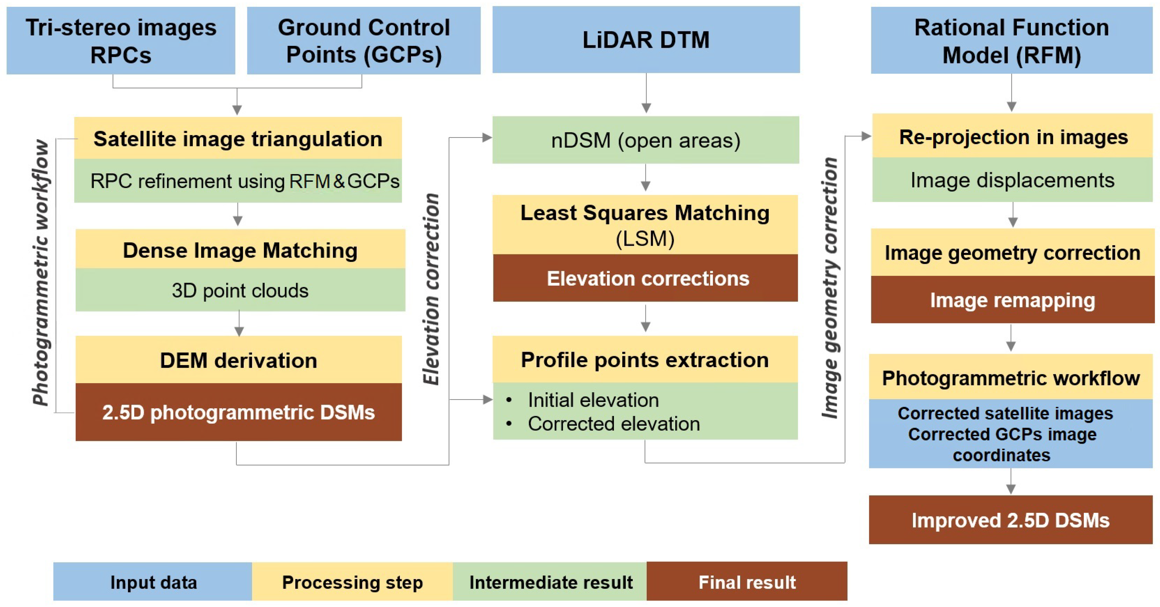
An overview of our processing pipeline is shown in Figure 1. Starting from raw satellite tri-stereo images (described in Section 2.1), we first perform an RPC bias compensation with GCPs followed by 3D reconstruction to obtain a DSM for each stereo pair (Section 2.2). A high resolution Lidar DTM is available in the area, therefore, the resulting DSMs could be improved by means of the global Least Squares Matching (LSM) technique in object space (Section 2.3.1). In this step, an elevation correction function is also determined by using the continuous LSM technique. The image correction functions are computed based on point re-projections (Section 2.3.2) and finally the corrected images and GCPs are employed as input for a new photogrammetric workflow, resulting in satellite-based DSMs with an improved quality.
2.1. Satellite Image Acquisition, Lidar DTM and GCP measurement
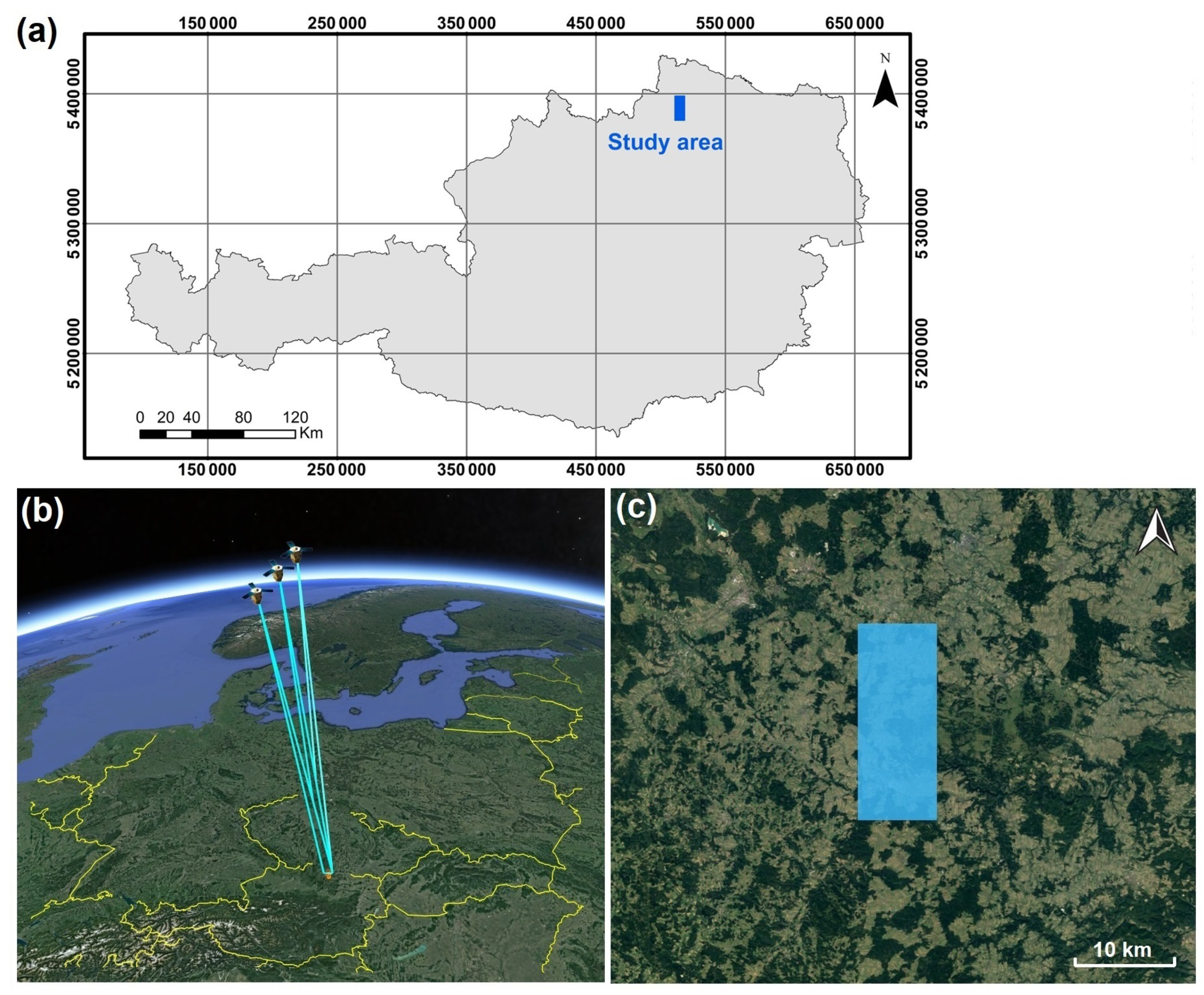
For the present experiments, a stereo triplet of Pléiades-1B satellite images acquired in the late morning of 13 June 2017 was used. This consists of three images collected during the same pass from different along-track positions of the satellite: forward (F), close to nadir (N), and backward looking directions (B). Due to the high platform speed (7.5 km/s) the sensor was able to cover a surface on the ground of 159 km within only 23 s. The Allentsteig study area is located in Waldviertel, Lower Austria (48°30′30″N; 15°08′34″E; WGS84), the north-eastern state of the country, a hilly region with elevations ranging from 537 to 846 m above sea level (Figure 2). From the total extend, about 47% is covered by arable lands, grasslands and agricultural fields, while about 39% is represented by coniferous and broad-leaved forests. Urban, suburban and rural areas are also present (for example Allentsteig and Zwettl cities, Niedernondorf and Scheideldorf villages), but they cover only small parts, compared with the entire area extend.
The three optical satellite images were provided as 16 bit pansharpened with four spectral bands (Red, Green, Blue and Near-infrared) at sensor processing level. Detailed information regarding the main acquisition properties are summarized in Table 1. The names of the images used in this research (and reported in the third column) follow the satellite viewing geometry, according to the off-Nadir viewing angle and acquisition time. Depending on the viewing angle, the ground spatial resolutions (mean values for the GSD) for Pléiades images vary between 0.70 and 0.71 m. The B/H ratios are of 0.13, 0.11, and 0.24, leading to convergence angles on the ground of 7.5°, 6.3°, and 13.8° for the forward-nadir, nadir-backward and forward-backward image combinations, respectively. Each satellite image was delivered with auxiliary data containing the RFM coefficients that allow the transformation between object and image space for subsequent photogrammetric processing.
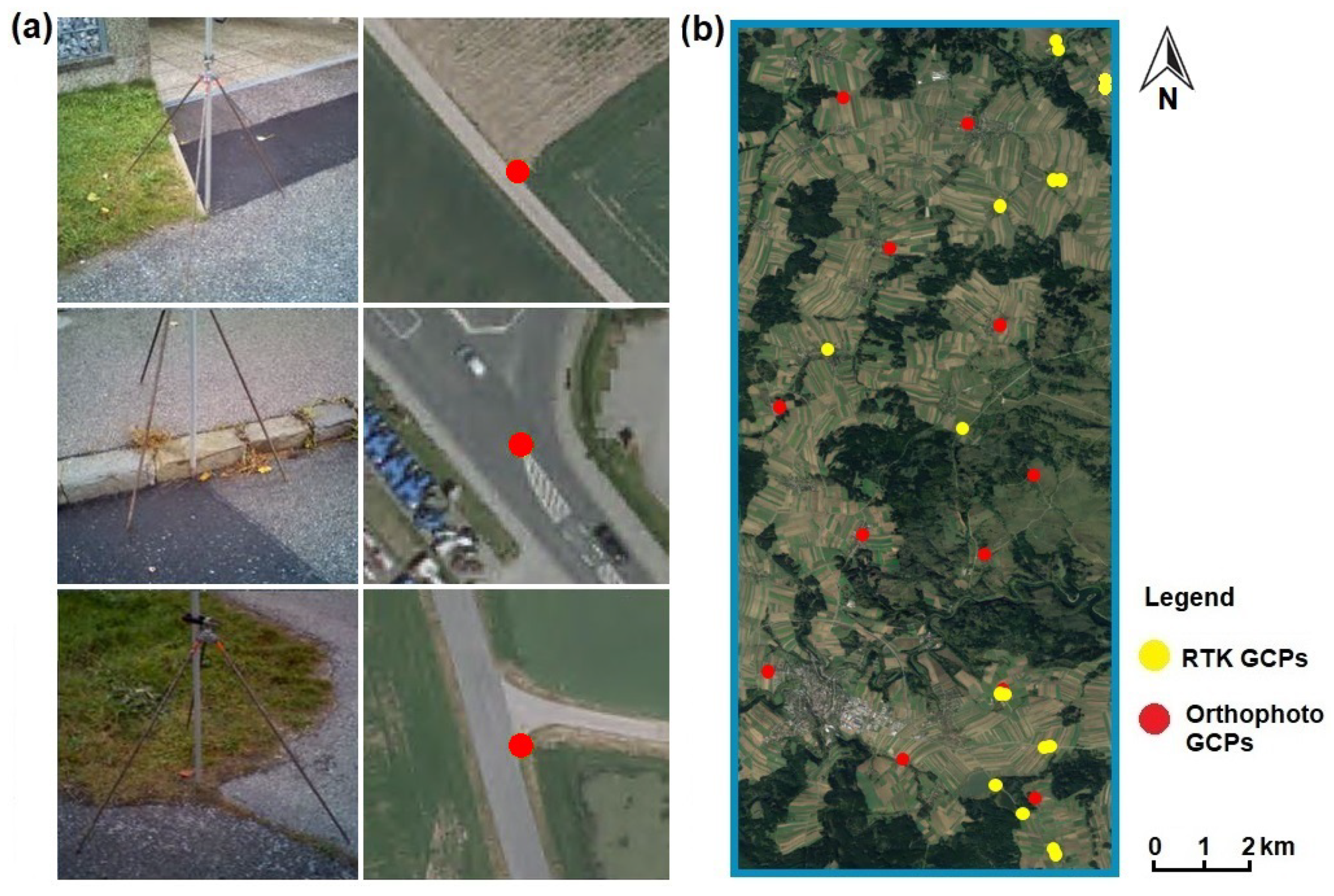
In order to refine the rational polynomial model and to check the accuracy of the final products, reference ground control is needed. For our study site, different reference data are available: GCPs, DTM from Lidar data, and a digital orthophoto. A set of 31 GCPs was directly measured in the field using GNSS real time kinematic positioning (RTK) with an accuracy of approximately 1 cm. Besides the improvement of satellite image georeferecing, the GCPs are used to check the punctual accuracy of the photogrammetrically derived elevation models. For the open, free area accuracy analyses, the DTM from Lidar was employed. With a spatial resolution of 1 m, the DTM was derived from an ALS flight measurement campaign in December 2015. Its vertical accuracy was checked against the RTK GCPs showing a of 0.12 m. Besides accuracy assessment, the Lidar terrain model was used to compute a reference mask for the open, smooth surfaces, and to improve the absolute geolocation of the satellite-based DSM by our proposed method. The planimetric accuracy of the available digital orthophoto from 2017 at 0.20 m spatial resolution was checked by computing the differences between the RTK point coordinates and their corresponding position in the orthophoto. The obtained result showed no shifts larger than one pixel. In order to obtain a homogenous distribution over the entire area of interest, additional GCPs were defined in the digital orthophoto, whose corresponding heights were extracted from the reference Lidar DTM at the same location. The positions of the newly defined GCPs were selected in such a way that they are visible in both the orthophoto and terrain model and they are identifiable in all the three satellite images. Moreover, the new points are located at the ground level, describing stable features in time with a high color contrast in the images. Hence the new manually measured GCPs are located at street marks (e.g., pedestrian crossing lines), intersections and road surface changes, corners and intersections of sidewalks, corners of paved areas and parking lots, parking space lines and intersections of these lines. Besides the available 31 RTK GCPs, 12 orthophoto GCPs were additionally manually measured (Figure 3).
2.2. DSM Derivation and Accuracy Assessment
The photogrammetric workflow as applied in this study starts with the Pléiades satellite image triangulation and dense image matching, followed by 3D information extraction and DSM derivation (Figure 1). As the image georeferencing phase is of primary importance for subsequent processing, the Pléiades triplet was oriented through the rational function model based on the eighty polynomial coefficients provided by the supplier. The reported geo-location accuracy for the Pléiades RPCs is 8.5 m CE90 (circular error at 90% confidence) corresponding to the nadir view [53]. However, as recommended, the geometry needs an improvement [54,55]. In order to reach a higher sensor orientation accuracy (to sub-pixel level), the model was further refined within a bias-compensation procedure by using GCPs and automatically extracted Tie Points (TPs), well distributed in the study area.
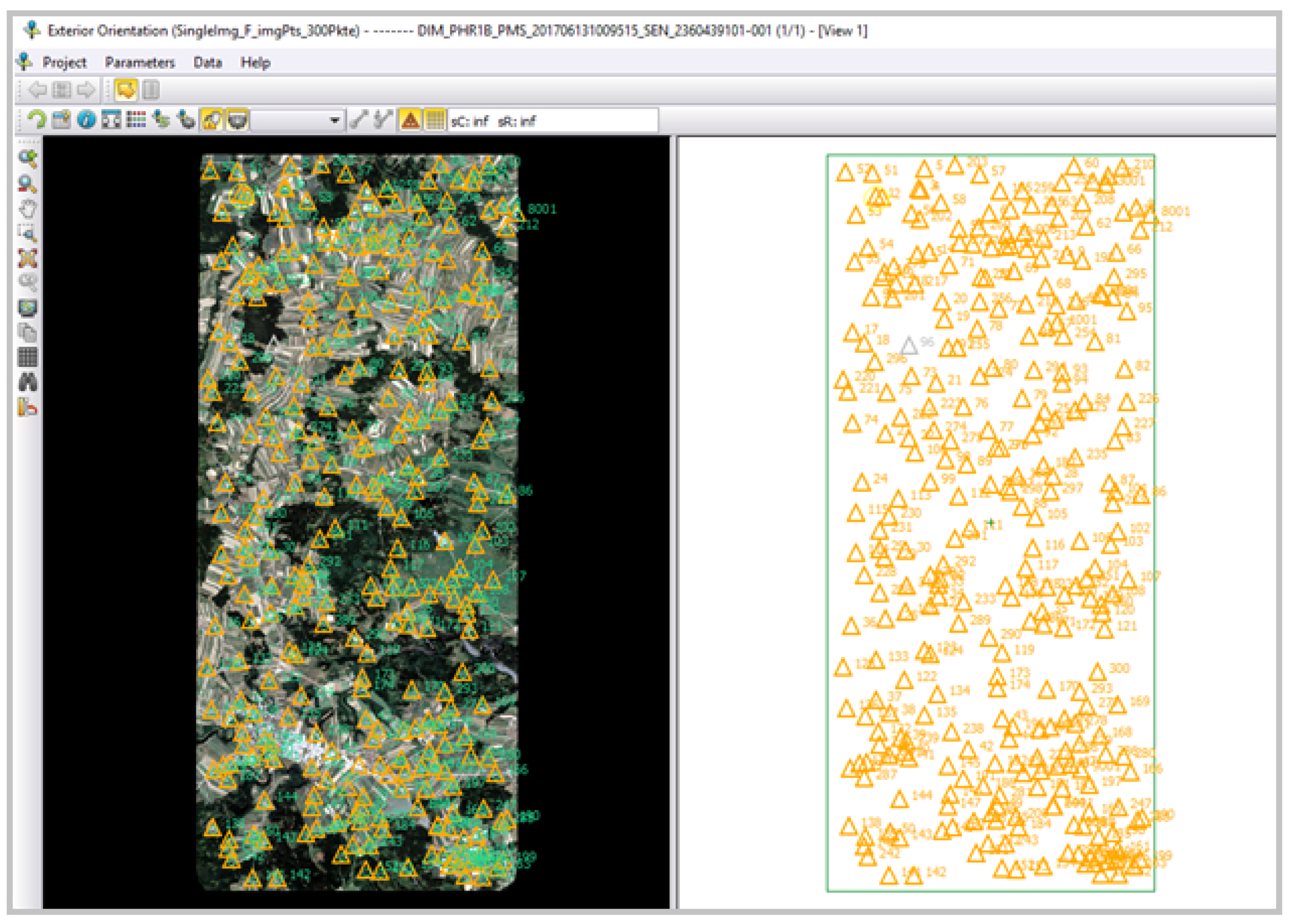
To assure a sufficiently good satellite image orientation and to check if systematic errors can be compensated by residuals in image space, we used a higher number of GCPs for refining the provided RPCs, with no automatic extraction of TPs. The considered investigation makes use of 300 GCPs (the previously defined orthophoto 12 GCPs were kept and an additional 288 orthophoto GCPs were measured) homogenously distributed over the Allentsteig scene (Figure 4). Their positions were defined based on the reference orthophoto and the corresponding heights extracted from the Lidar DTM. The 2D image coordinates of the GCPs were manually measured using the software SAT Master from Inpho/Trimble, which allows a simultaneous display of the images. To evaluate the accuracy of the georeferenced images, the RMSE between the adjusted coordinates (provided by the software) and the originally measured coordinates were computed, resulting in an overall RMSE of the residuals well below one pixel.
The photogrammetric process was completed by deriving surface points using image matching via the software Match-T DSM from Inpho Trimble (Version 9.2). The adopted matching strategies are based on Least Squares Matching (LSM), Feature Based Matching (FBM), and Cost Based Matching (CBM). The outputs are dense photogrammetric point clouds with three-dimensional coordinates in object space (i.e., X, Y, Z) and reflectance information from the three spectral bands (Red, Green and Blue). In LAS file format and with a regular distribution (one point per each image pixel), the reconstructed point clouds have densities of circa 1.42 points/m. Dense image matching was performed for each stereo pair i.e., forward-backward (FB), forward-nadir (FN) and nadir-backward (NB) and in a last step, regular raster models of height values (DSM) at 1 m resolution are generated using a robust moving planes interpolation. A search radius of 2 m and a maximum of 10 nearest neighbours are used for the interpolation. According to the input point density, we have chosen this as the optimal approach in terms of surface detail preservation.
The accuracy (in planimetry and elevation) of the satellite-based DSMs was evaluated by comparing the GCPs’ coordinates (measured either on the ground or on orthophoto and Lidar) with those monoscopically measured on the oriented satellite images in a multi-image view-mode. The summary of the resulted statistics for the coordinates are then visualised with boxplots.
The vertical accuracy assessment of the reconstructed DSMs was determined against the available elevations of the GCPs and reference Lidar DTM in open areas. Hence, the vertical accuracy was determined by: (1) computing the RMSE between reference and extracted elevations from each generated DSM for the GCPs; (2) visually analysing the difference elevation models (color-coded by elevations with corresponding color palettes) and (3) analysing the distribution histogram of difference values, by deriving statistic parameters such as mean, median, standard deviation, robust standard deviation () and RMSE. After quality checking, systematic errors were visible between the reconstructed DEMs and the Lidar DTM. Therefore, an improvement strategy is required.
2.3. Satellite DSMs’ Improvement
Obtained through photogrammetric processing, the satellite-based digital elevation models can be further improved by adopting several techniques. These can be either applied in object space (like the LSM technique) or in image space (through our proposed methodology).
2.3.1. Least Squares Matching Technique
As a traditional photogrammetric technique used for establishing correspondences between images collected from different viewing points (or between consecutive images of a sequence), LSM determines the parameters of an affine transformation between corresponding patches of two or more images. Formulated for two-dimensional greyscale images [56], the technique can be applied to surface models with a grid structure, as well [57,58,59]. In this case, LSM acts very similarly, by estimating an affine 3D transformation to align overlapping elevation models. The main idea is to find the corresponding location of a surface patch inside a window of one dataset in another dataset. This is usually undertaken by estimating a transformation in such a way that the differences between the two input models inside the patch are minimized. In contrast to images, where the defined LSM patch size should be limited to small windows (due to different viewing directions and perspective image projection), LSM can be applied to satellite- or ALS-derived elevation models over large areas (due to the orthogonal projection of the models).
In our investigation, the LSM technique is used in two different ways:
- Global LSM—for global improvement of the georeferencing of photogrammetrically derived DSMs.
- Continuous LSM—for modelling the periodic systematic elevation errors (waves) in object space (described in Section 2.3.2).
Applied to the photogrammetrically derived DSMs, the global LSM technique estimates an affine transformation between each input elevation model and the reference Lidar DTM over common open surfaces. For a reliable transformation estimation, some specific areas were not included during LSM, because of vegetation cover, matching errors and/or occlusion. Hence, from the input surface models, areas containing vegetation, rivers, lakes, buildings and other artificial objects on the ground were masked out. For this purpose, an above-ground mask was computed by using the volume-based algorithm developed by Piltz [60], having as input the photogrammetric sattellite DSM. Therefore, only smooth, object-free stable surfaces (called open areas in the following) were considered for the computation. Here, the differences in height between DSM and DTM are expected to be as low as possible (below 10 cm).
In the case of the Allentsteig study site, the percentage value of open areas (as stated before) within the Pléiades dataset is of approximately 37.8%. The affine 3D transformation with 12 parameters can be expressed in the following form:
where is the point given in the system of the dataset to be transformed (DSM), is the same point given in the system of the fixed reference dataset (Lidar DTM), is the reduction point, the translation vector and the rotation matrix given by:
Performed for open areas, the global LSM technique estimates a single global transformation parameter set, which is subsequently used to transform the Pléiades DSMs to the Lidar DTM. In contrast to global LSM where large open areas are considered for the computation, the continuous LSM technique [58] uses smaller patches arranged along flight direction for modelling the periodic systematic elevation errors. Both LSM modes, global and continuous, were conducted in the scientific software OPALS (Orientation and Processing of Airborne Laser Scanning Data) [61].
2.3.2. Image Geometry Correction
The proposed method for computing the satellite image geometry corrections employs a higher resolution elevation model (like in our case a Lidar DTM). The fully integrated methodology is depicted in Figure 1 and comprises three main steps:
- Photogrammetric processing;
- Elevation difference computation;
- Image geometry improvement.
The first part describing the photogrammetric processing chain with bias-compensation of the RPCs using GCPs for deriving elevation models from satellite imagery is detailed in Section 2.2.
Secondly, the elevation corrections in object space are determined by applying the continuous LSM photogrammetric technique between satellite-based DSMs and the reference Lidar DTM in open, smooth areas. The continuous mode option of LSM uses small patches arranged along the flight direction with the patch length as the dimension measured along the flight direction and the patch width represented by the dimension measured perpendicularly to the flight direction. For modelling the periodic systematic elevation errors in object space, the continuous mode option of LSM was used with a patch length of 1200 pixels and 70% overlap between successive patches (360 m forward movement). The patch width (across the flight direction) extends over the entire overlap. This continuous mode option of LSM in the software Opals is executed in a robust way. In this way the differences induced by objects (e.g., vegetation or buildings) between the reference DTM from Lidar and the DSM from the satellite images are removed (as long as enough open terrain is contained in the sliding window during continous LSM). Finally, an individual transformation parameter set (offsets in Z direction) is estimated for each patch. Hence, the elevation corrections describe the offsets in Z direction as a function of Y coordinate (i.e., in flight direction):
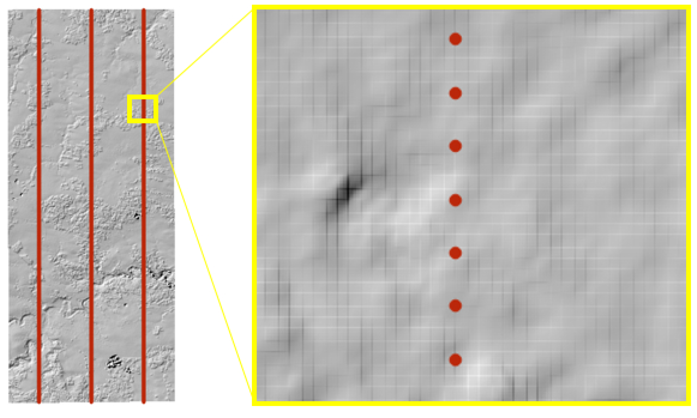
Thirdly, the image geometry corrections are determined by adopting a “from object to image space” re-projection procedure. The image correction starts with the extraction of 3D point profile lines. The selected points are distributed in three parallel lines at 10 m intervals along the flight direction. In total, the 2D positions (latitude, longitude) of 5583 points (1861 in each line) are defined (Figure 5). Their corresponding elevations (Z) are extracted from the photogrammetric satellite-based pairwise DSMs (FB, FN, NB) and the corrected elevations are computed using the function of Z differences resulting from the LSM-continuous approach with the following formula (for an object point with coordinates ):
where is the correction function for Z elevation differences in Y-coordinate direction (as resulting from continuous LSM for each DSM model: FB, FN, NB).
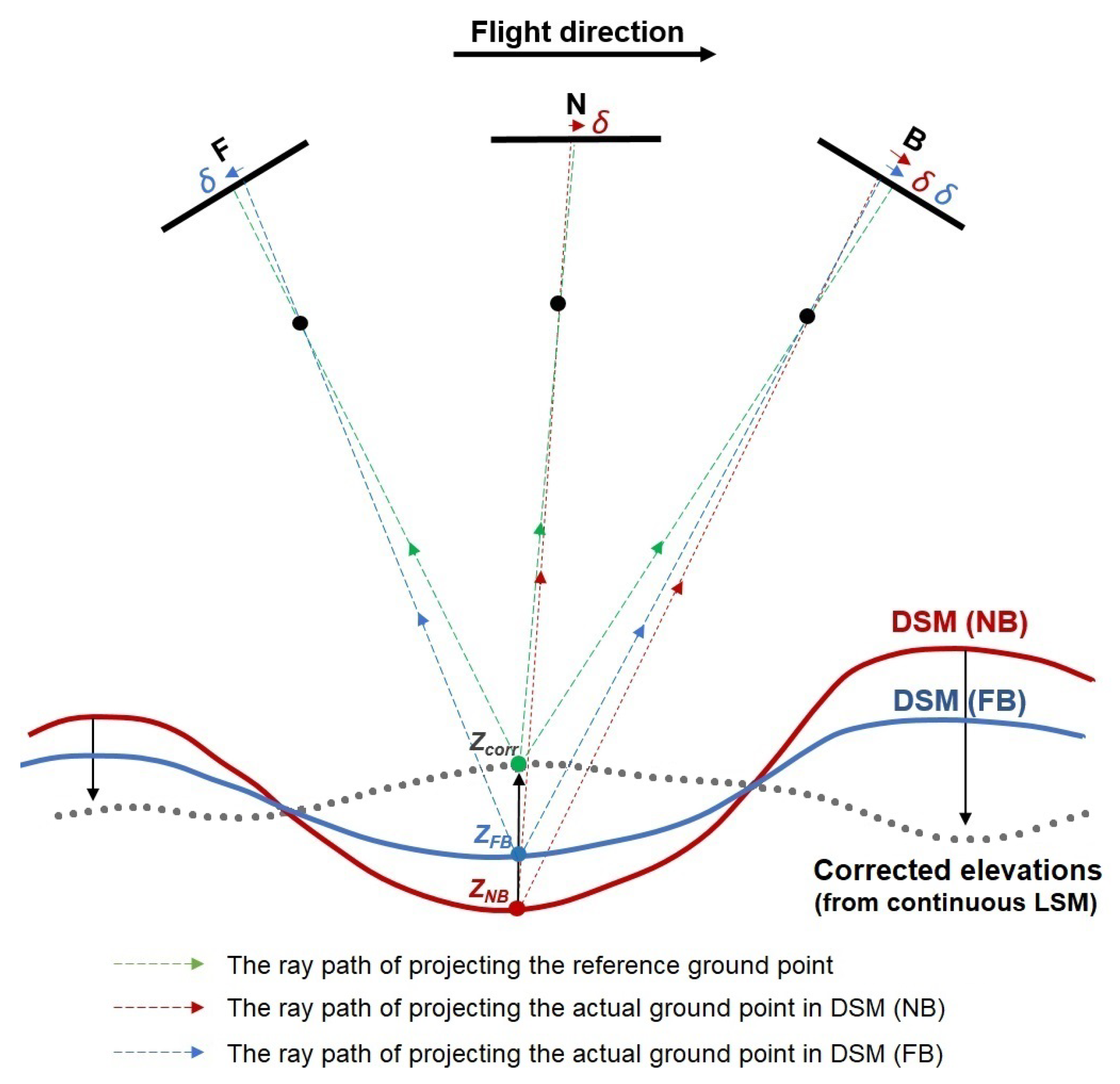
Following the mentioned principle “from object to image space”, the 3D points from line profiles are projected into the image space using the RPC model (Figure 6).
For each 2D point position from the three profile lines, two different elevations are available: (1) elevations extracted from the pairwise satellite-based DSMs (FB, FN, NB) and (2) the corrected elevations (computed in a previous step by applying the elevation correction function resulting from continuous LSM). By re-projection to the image space, the points have different positions in the satellite images and thus, the resulting displacements serve as the basis for the computation of image corrections, by using the following general formula:
where —3D point coordinates with Z extracted from the satellite-based elevation model showing systematic errors, —row, column image coordinates, —3D point coordinates with corrected Z elevation, —corrected point position in image space, —image correction (displacements, computed as the difference between the corrected and initial row point position in image space).
In contrast to stereo, the tri-stereo satellite image acquisition allows the computation of pairwise DSMs and, therefore, each satellite image is involved in the derivation of two pairwise DSMs: Forward image in , , Nadir image in , , and Backward image in , . Hence, two different correction functions per satellite image are computed, which are averaged in a final stage. Additionally, the distribution of points in three profile lines requires the estimation of average corrections. For example, the computation of satellite correction function for the Backward image, implies the following calculations:
- (1)
- Re-projection of 3D points in image space
The procedure is described for the Backward image, but applied to the other two scenes analogously.
where and —3D coordinates of points extracted from satellite-based elevation models, and —image coordinates in Backward scene, —3D point coordinates with corrected Z elevation, —corrected point position in Backward image.
- (2)
- Corrections in image space
- (3)
- Correction average of profile point lines
- (4)
- Final average correction model for Backward satellite image
The implementation of the computed correction models to each satellite image implies a replacement of pixels from one location in the source-image to the correct location in the final image, a process called warping. This strategy is possible by using the specific remap() function from the OpenCV library. Since a perfect one-to-one-pixel correspondence between source and destination images is not achievable, a cubic interpolation was set for non-integer pixel locations. The correction for every pixel location is expressed as:
where is the remapped image, the source image and is the mapping function that operates on , given by:
where the mapping function remains constant in the column direction (which for Pléiades corresponds nearly to X-East direction), while the defines the image correction function model for displacements in the row direction (corresponding to Y-North direction). This function is sampled over the final average correction model (Equation (9)) with a pixel spacing on the ground of approx. 10 m/0.7 m.
The image correction model was not applied to the satellite images only, but also to the coordinates of the GCPs in image space, where the coordinates (c, r) in the remapped image are derived as:
3. Results
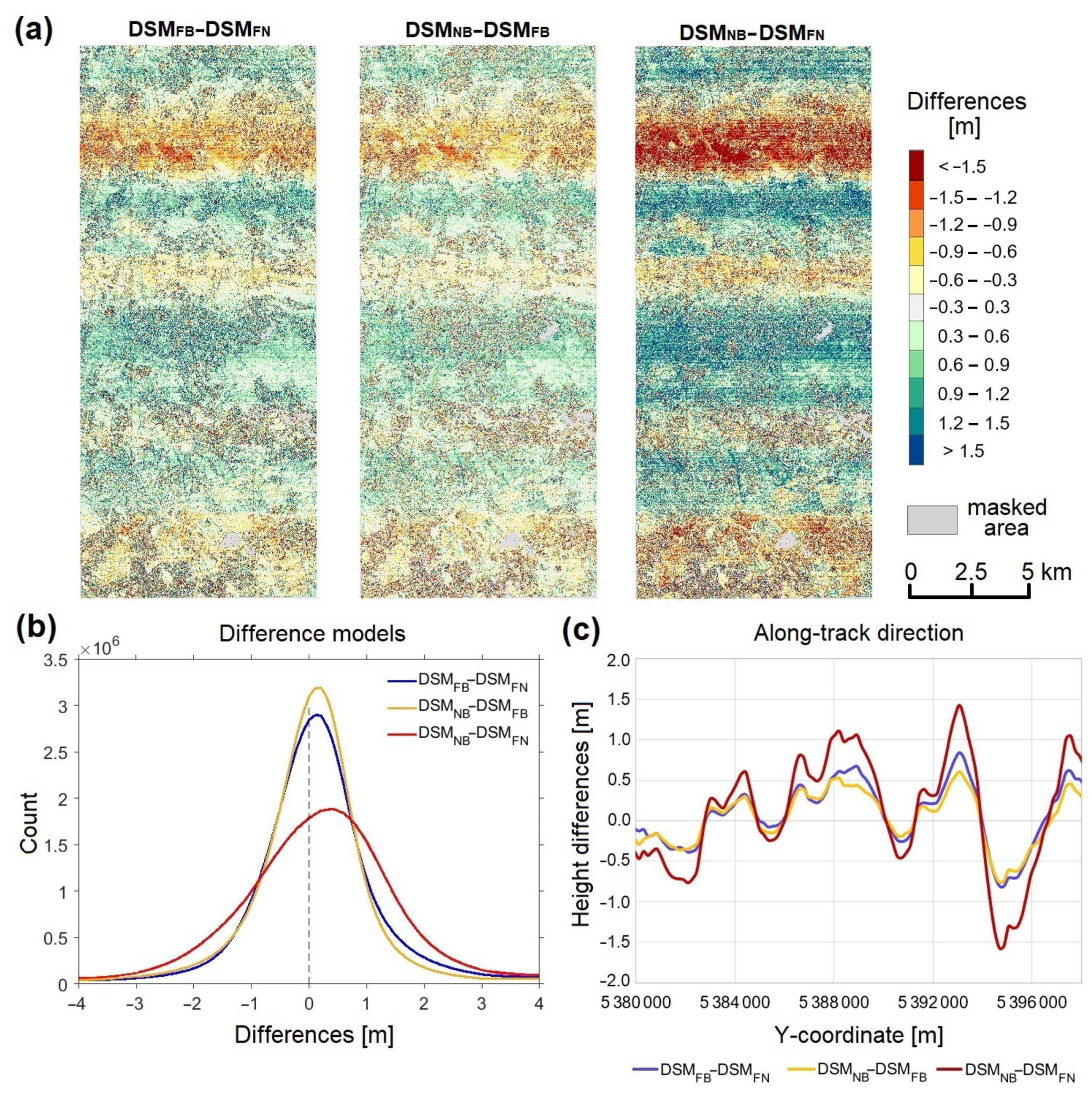
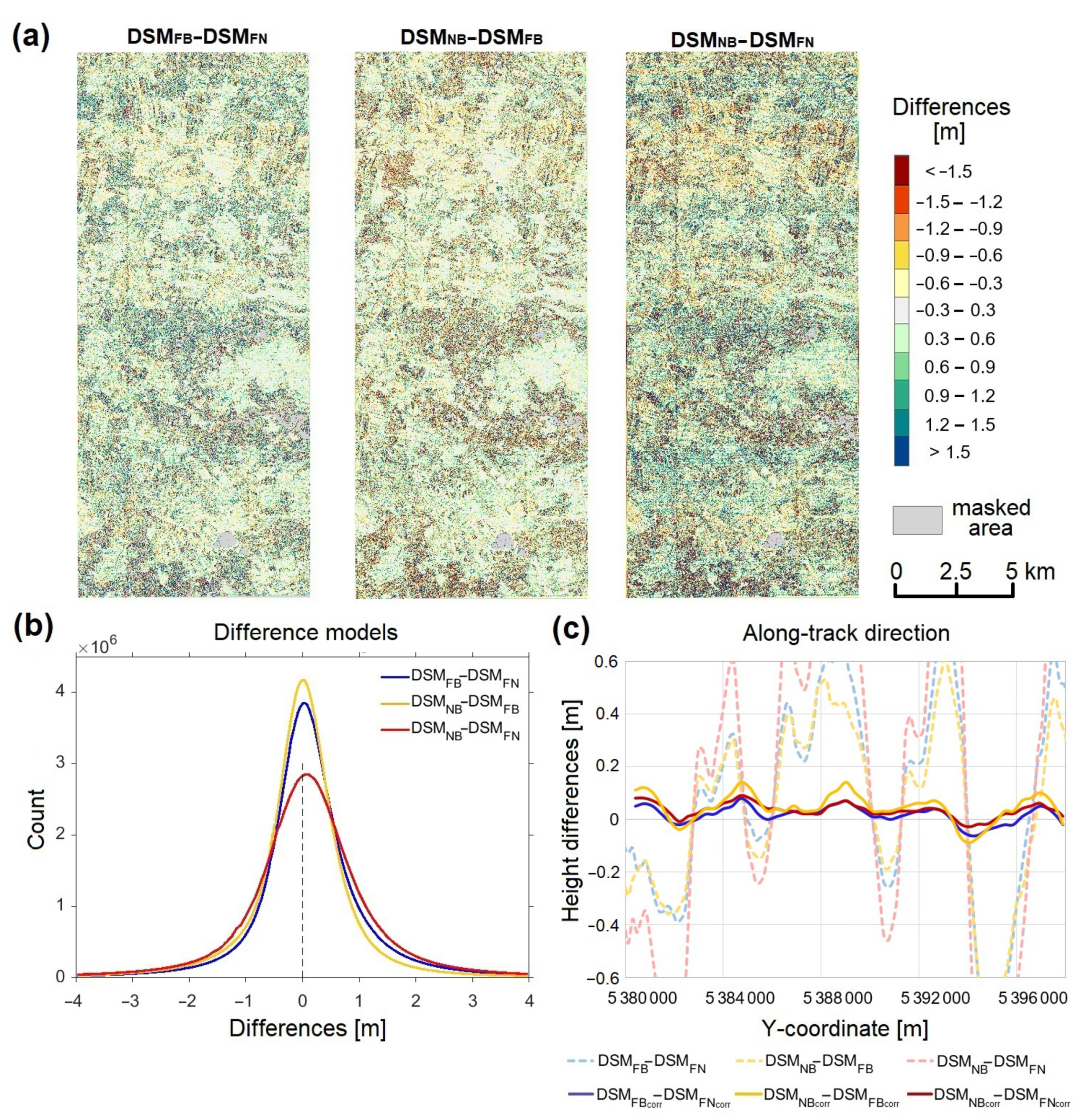
In this article we investigate triple stereo scenes. In comparison to a stereo pair, this offers the possibility to build three image pairs to compute a surface model. With perfectly calibrated and oriented images all three surface models deviate from a reference model, but also from each other only by random errors. As Figure 7 shows, this is not the case for the investigated data. A surface model computed from all three images shows differences to the Lidar reference model as systematic deviations with an amplitude reaching 0.88 m. These differences can only be determined, if a reference model of higher (bias free) accuracy is available. In our case, we consider the Lidar DTM as a bias-free reference model, since it was checked against the measured GCPs showing a good vertical accuracy with a standard deviation value of 0.12 m. Additionally, the systematic effects of satellite elevation models do not appear when computing the differences to the Lidar model only, but also between the surface models computed between the different pairs, which show even stronger systematic wave-shaped patterns, as demonstrated in Figure 8. In this case, the elevation differences for , and reach amplitudes of 0.87 m, 0.78 m and 1.65 m, respectively. In following analysis we investigate these effects and propose possible remedies for improvement.
3.1. Satellite-Based DSM from Image Orientation with Bias-Corrected RPCs Using 43 and 300 GCPs
3.1.1. Image Orientation Results
For an accurate processing, the satellite image orientations provided through the RPCs were improved by estimating an affine transformation in image space, making use of available GCPs. Two situations were analysed:
- (1)
- Image georeferencing with bias-corrected RPCs using 43 GCPs and automatically extracted TPs
- (2)
- Image georeferencing with bias-corrected RPCs using 300 GCPs (no TPs are involved).
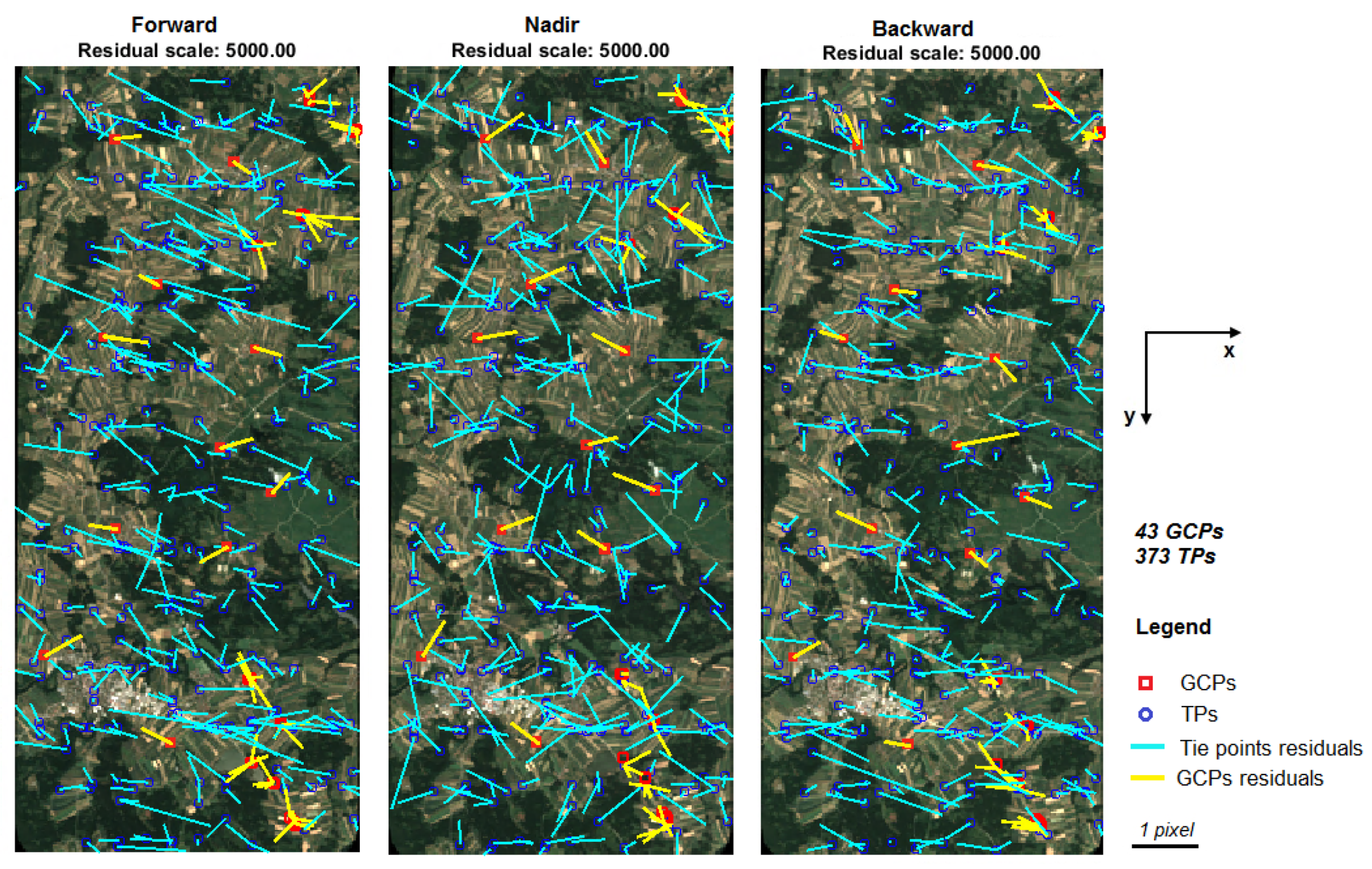
The error vector plots in image space (for GCPs and TPs) resulting from satellite triangulations in the two cases are shown in Figure 9 and Figure 10 and statistics are given in Table 2.
In both image block-orientations, values in the range of 1/3rd of a pixel were achieved for the standard deviations of point residuals. When looking at the statistics for image residuals of GCPs and automatic TPs, generally the values in the cross-track direction (x-residual) are larger than those in the track direction (y-residual). Assuming that the epipolar lines are approximately parallel to the flight direction, this indicates a good estimation in the cross-track (cross epipolar line) direction, but less control in the flying direction, keeping some systematic errors. Moreover, when comparing the RMSE y-residual within the Allentsteig image triplet—0.13 pixels, 0.22 pixels, 0.12 pixels in the first case (RPC bias-correction with 43 GCPs) and 0.24 pixels, 0.38 pixels, 0.31 pixels in the second case (RPC bias-correction with 300 GCPs) for Forward, Nadir, Backward images—larger value for the Nadir image suggests a better estimation of the orientation in comparison to the Forward and Backward scenes. This effect will also be proven by the smaller correction values for the Nadir image in Section 3.3.1. No systematic component in the y-direction can be observed for the image point residuals obtained based on bias-corrected RPC orientation using 43 GCPs (Figure 9).
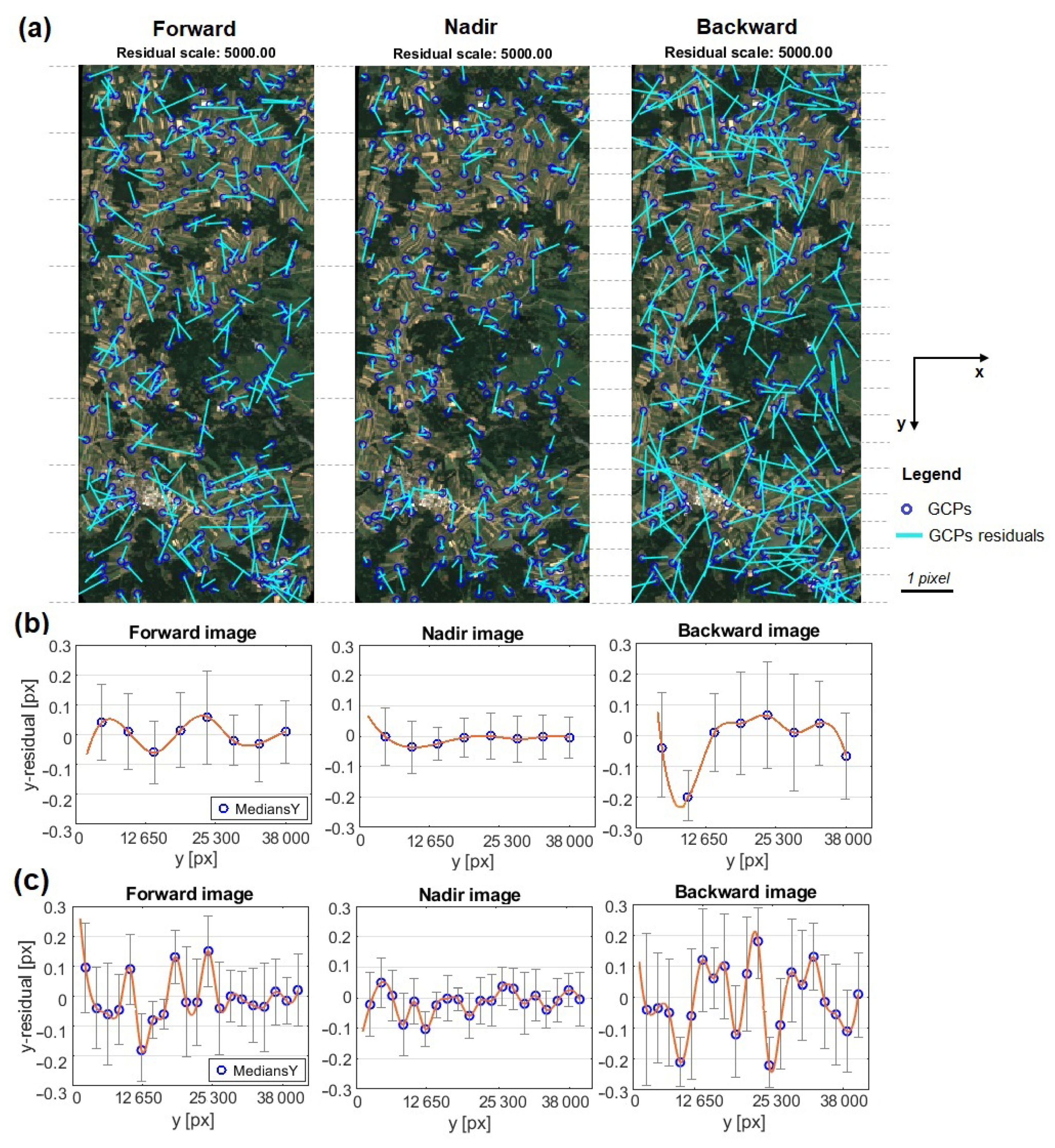
In the second case, satellite image orientation was performed with bias-corrected RPCs using 300 GCPs (no TPs included). Figure 10 provides an insight into the question of modelling the systematic error in the along-track direction (y), by making use of residuals’ robust statistics, such as median and standard deviations. The basic idea was to group the y-residuals in equal intervals along the track direction and check if the median values of the frequency distribution in each interval show similar patterns, thus deviating from a purely random distribution. However, the resulting graphs per each image displaying the medians in the y-direction and robust standard deviations for eight intervals (Figure 10b) do not show regular oscillations. While the Forward image has two complete oscillations, the Nadir graph is mostly flat and the Backward graph is irregular. By increasing the number of intervals along the track direction, the robust standard deviations remain mostly constant: between 0.1 and 0.15 pixels for Forward, smaller than 0.10 pixels for Nadir, and between 0.15 and 0.25 pixels for Backward. The high variability of medians-Y values leads to the conclusion that the 300 GCPs are not suited for identifying systematic errors from image residuals, therefore, a digital elevation model is needed. Apparently, the quite random distribution of the GCPs’ coordinate residuals in image space (showed as vector plots in Figure 10) suggests the absence of any further systematic error.
3.1.2. DSM Accuracy Evaluation
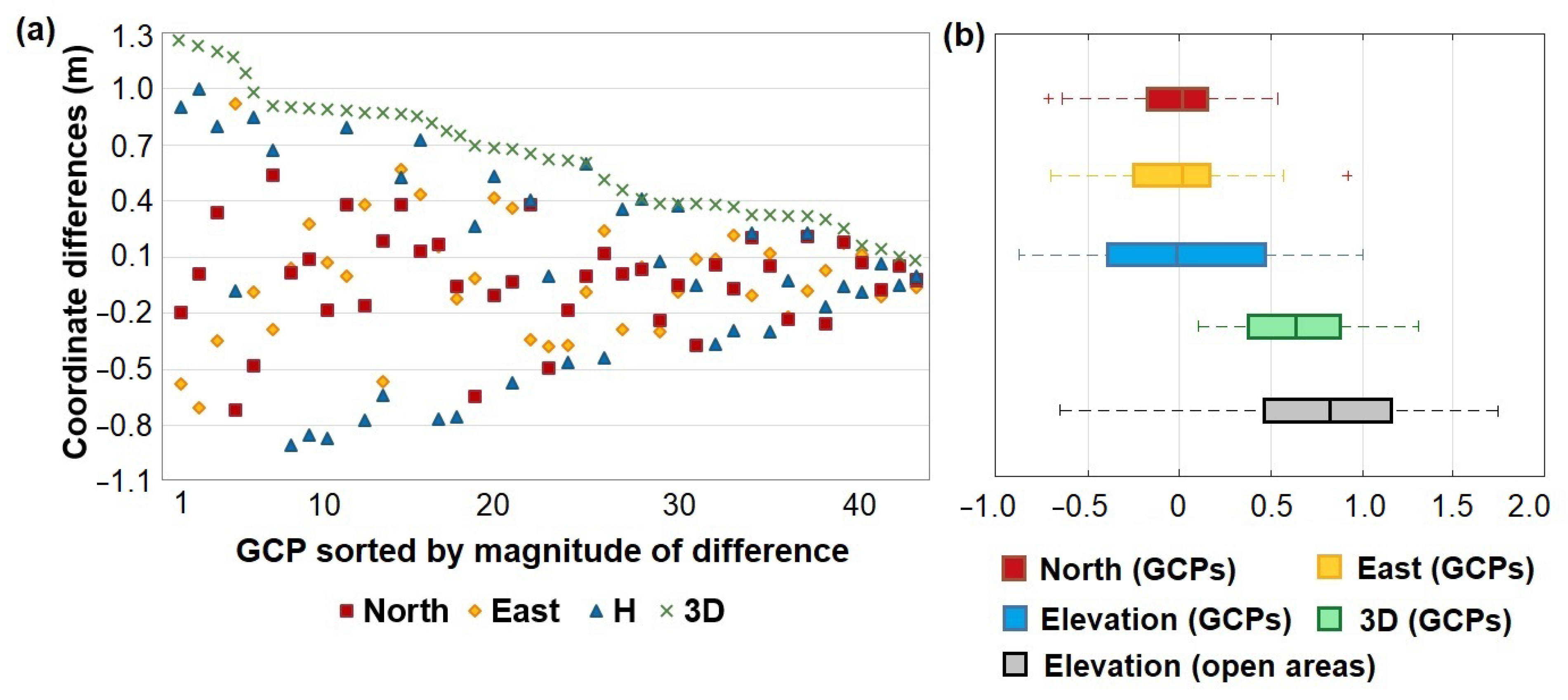
The accuracy of the computed satellite imagery aerial triangulation was evaluated by comparing the GCPs’ coordinates—measured directly on the oriented satellite images—with those measured on the terrain (or extracted from the orthophoto and Lidar). Statistic results for the 43 GCPs are shown in Table 3. Figure 11 shows the graphs of comparisons at GCPs, where the coordinate differences are less than 1 m for most of the points.
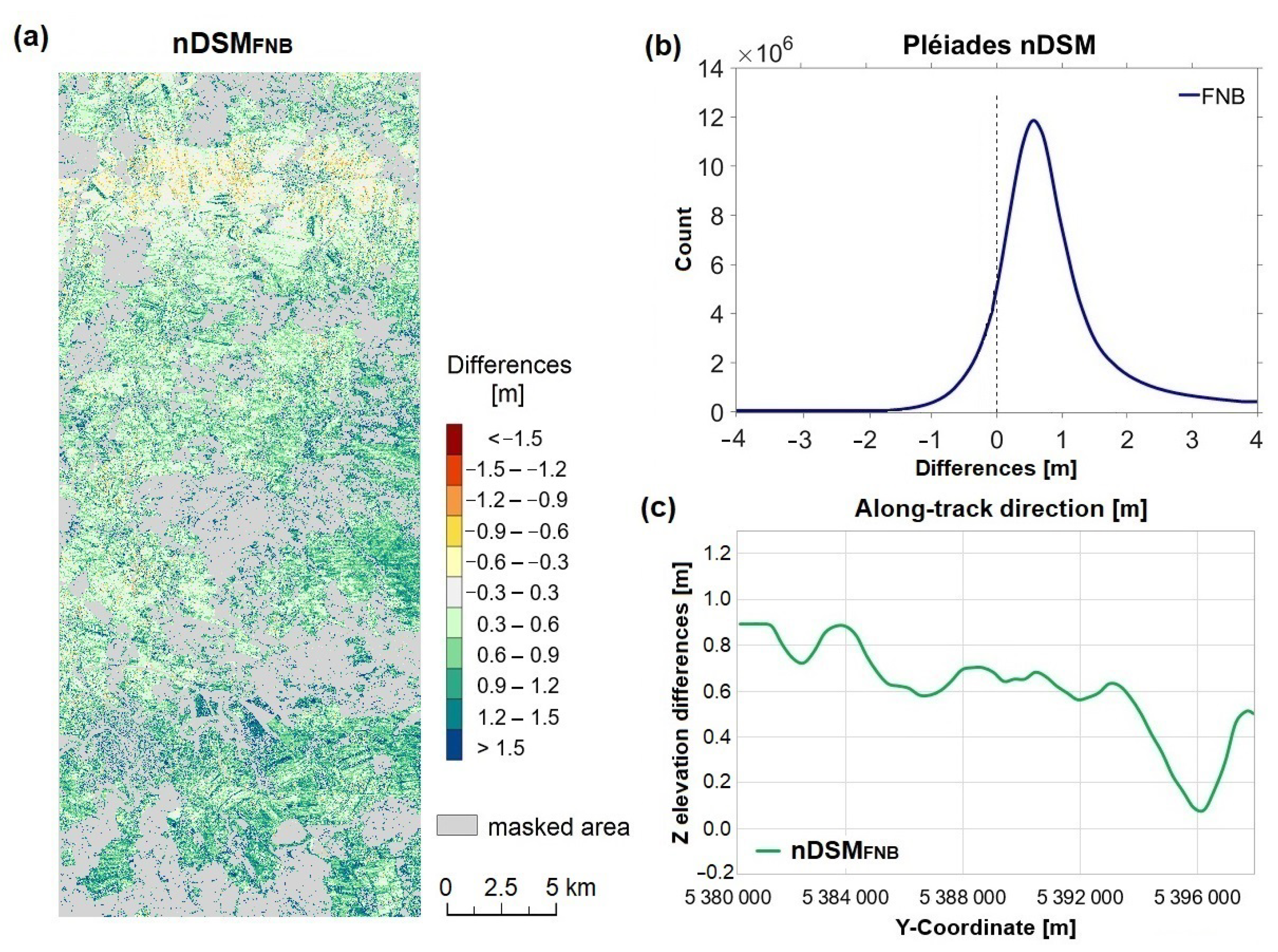
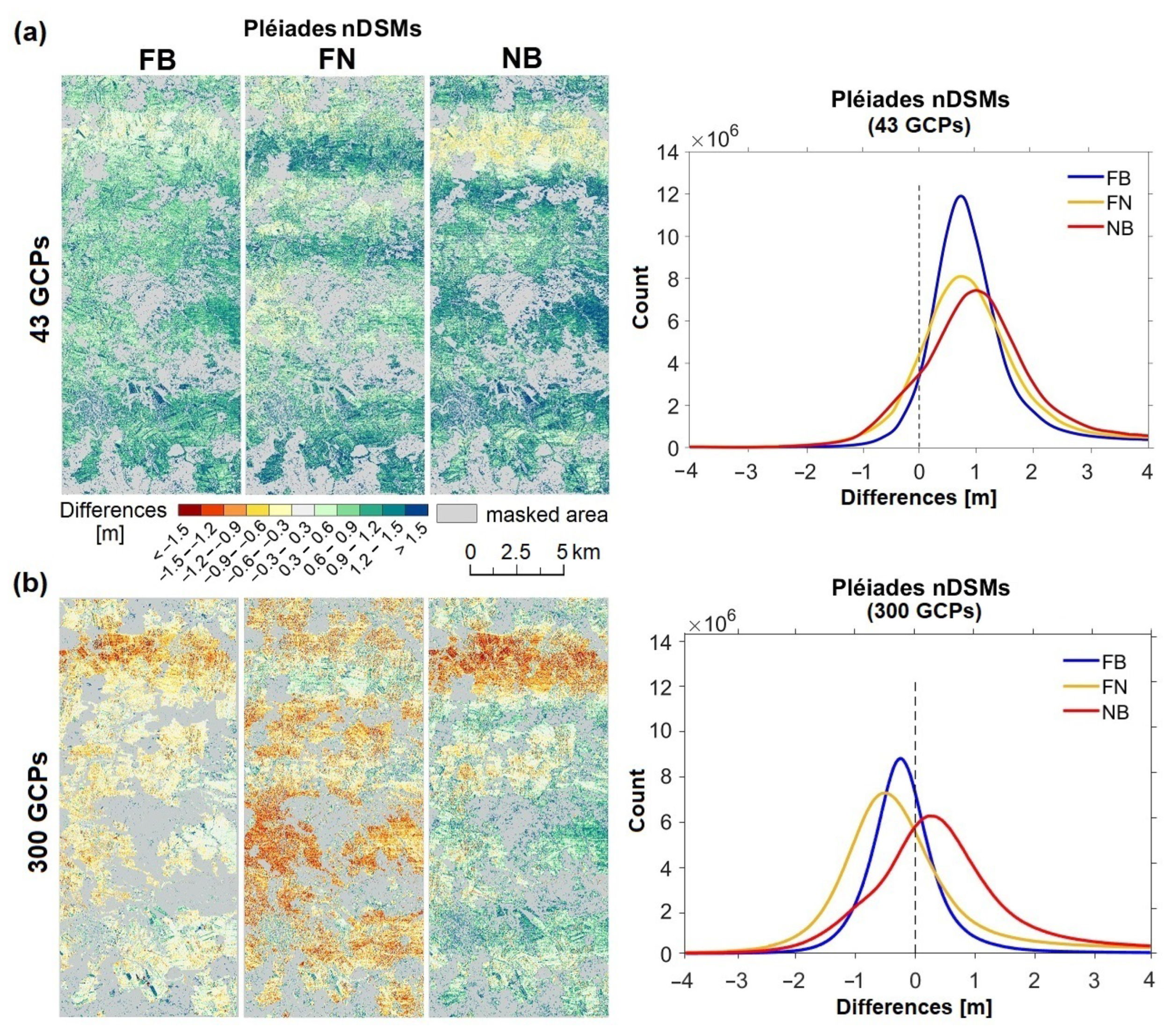
At a wider scale, the accuracy of the satellite-based DSMs was evaluated by comparing them with the ALS DTM reference data in open, free areas. Figure 12 shows a comparative view of the resulted nDSMs from the two investigations: RPCs refined with 43 GCPs and with 300 GCPs. In both cases, the color-coded height difference models reveal periodic systematic errors (similar to an undulation effect with waves) that are visible in the along-track direction. Statistics of elevation differences show non-Gaussian distributions of errors with a positive vertical offset of the Pléiades DSM (with approximately 1 m) over the reference Lidar DTM. In contrast, the elevation models computed with 300 GCPs show a better agreement with the Lidar DTM, with mean values close to zero and the best RMS of 0.65 m for the DSM from FB image combination (Table 4).
3.2. Satellite DSMs Corrected with LSM
In order to reduce the systematic errors in the satellite-based DSMs, we applied the global LSM technique between the satellite-based DSMs and reference Lidar DTM in open areas. From a visual inspection, after applying the LSM transformation we obtain an improved agreement between DSMs and the reference DTM, although the systematic wavy effect is still preserved (Figure 13).
The statistics of elevation differences between the satellite-driven DSMs (all combinations) and available reference model before and after applying the global LSM technique are given in Table 5. Initially systematically shifted by 1 m, the reconstructed terrain heights are reduced after applying the transformation. The global LSM technique substantially reduced the RMS values with 22% for FN and NB scenes, with up to 35% for FB scene.
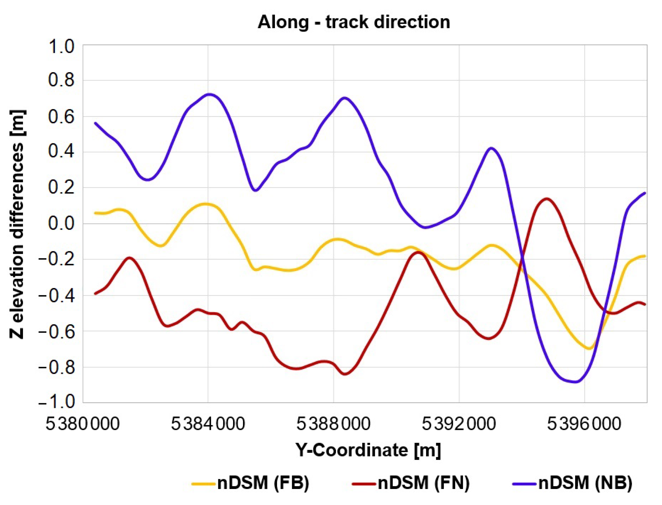
Computed with the LSM continuous approach, the elevation corrections describe the offsets in Z direction as a function of Y coordinate (in the flight direction) (Figure 14). The elevation differences from the FB surface model are around 0 m (they are the closest to 0 m, compared to NB and FN). While the maximum absolute difference for the FB model with respect to Lidar DTM is of 68 cm, the differences for NB and FN elevation models reach minimum values of −88 and −85 cm, respectively. Similar to oscillations, wavy patterns are visible in all three difference models, more pronounced in FN and NB, which have a symmetric appearance to the horizontal 0 m axis. The FB model is similar to NB, but with waves of smaller amplitudes.
3.3. Satellite DSMs Corrected Based on Image Warping
3.3.1. Image Correction Models
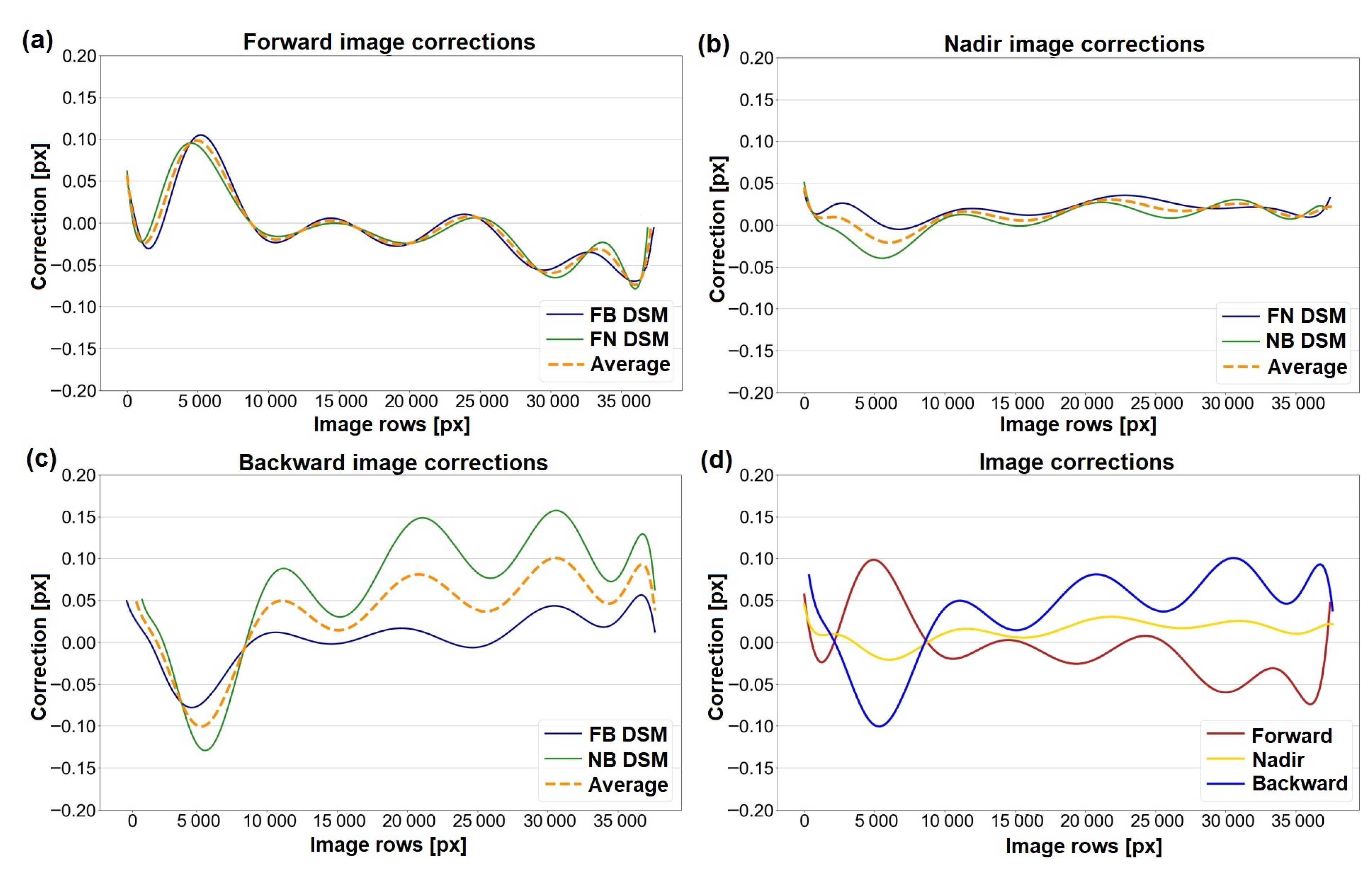
Since each satellite image is involved in the computation of two DSMs (Forward image in , , Nadir image in , , and Backward image in , ), two different corrections per image are obtained. The resulted correction functions and their average for the tri-stereo Pléiades satellite images are shown in Figure 15. For the Forward image, the correction functions computed from the two DSMs are very similar and fit very well together. For the Nadir image the amplitudes of the waves are also quite similar and the smallest (<0.02 pixels). The largest discrepancies are visible in the corrections corresponding to the Backward image. Even if the oscillation pattern is similar for both FB and NB DSMs, the correction function corresponding to the NB DSM has the maximum deviation from zero 0.125 pixels and valley-peak-span of 0.23 pixels, respectively. The resulting average image corrections for the tri-stereo Pléiades satellite imagery have amplitudes of maximum 0.063 pixels, 0.020 pixels, and 0.075 pixels for the Forward, Nadir, and Backward images, respectively. Overall, the average correction functions in all images are characterized by repetitive waves with lengths of 9509 pixels (wavelength = image rows/no. of waves, 38,034 pixels/ four waves), amplitudes varying between 0.012 and 0.075 pixels and heights between 0.025 and 0.15 pixels (Figure 15d).
A maximum wave height of 0.15 pixels corresponds to 10.5 cm on the ground. The image correction functions can be interpreted as describing the vibrations (jitter) of the satellite during image acquisition, by moving back and forth from its normal stationary position on the platform.
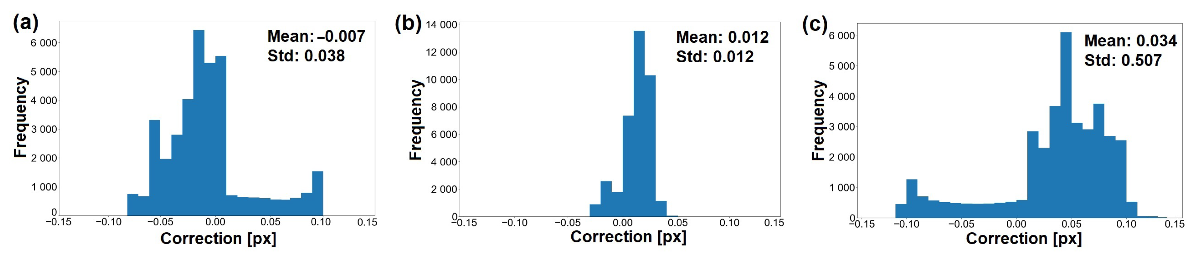
The distribution histograms for the corrections show higher values for mean and standard deviation in the Backward image when compared to the other two. The corrections for the Nadir image are the smallest, between −0.05 and 0.05 pixels (Figure 16).
When reversing the image rows (considering the opposite direction of rows from top to bottom in the image coordinate system with origin in top left corner), a similarity between image correction functions (Figure 15d) and the profile height differences for pairwise Pléiades nDSMs in object space (Figure 14) can be observed. The four dominant peaks in the correction models for each image correspond to the four peaks in the computed normalized difference surface models.
3.3.2. Sensor Oscillations
Describing oscillations with wavelengths of 9509 pixels, the determined image corrections reveal important technical information regarding the image acquisition w.r.t sensor rotation in time (pitch angle) and satellite oscillations. The sensor vibration i.e., change of the viewing direction from the sensor towards the ground for each wavelength can be determined by the following formula:
where y is considered the maximum wave amplitude of 0.15 px (0.105 m) and H the Pléiades satellite orbit height of 694 km. This results in a very small oscillation angle of the sensor with a value of degrees.
Based on the satellite image acquisition properties also, the time for a complete cycle of the oscillation (oscillating period T) can be computed. One satellite image (16,665 × 38,034 pixels) is acquired in less than 3 s (2.795 s Forward, 2.823 s Nadir, and 2.803 s Backward images), which typically results in a recording time of for each row-line. An oscillation with 9509 px wavelength (corresponding to 6656 m on the ground) is recorded in a time interval of 0.70 s. Knowing that frequency f refers to the number of waves per unit of time, given by f = 1/T, the satellite vibrations have a frequency of 1.42 Hz. Due to the small number of waves (the wavelength is very long w.r.t. the total extend), we directly measured the wavelengths from the data and did not derive them using Fourier analysis.
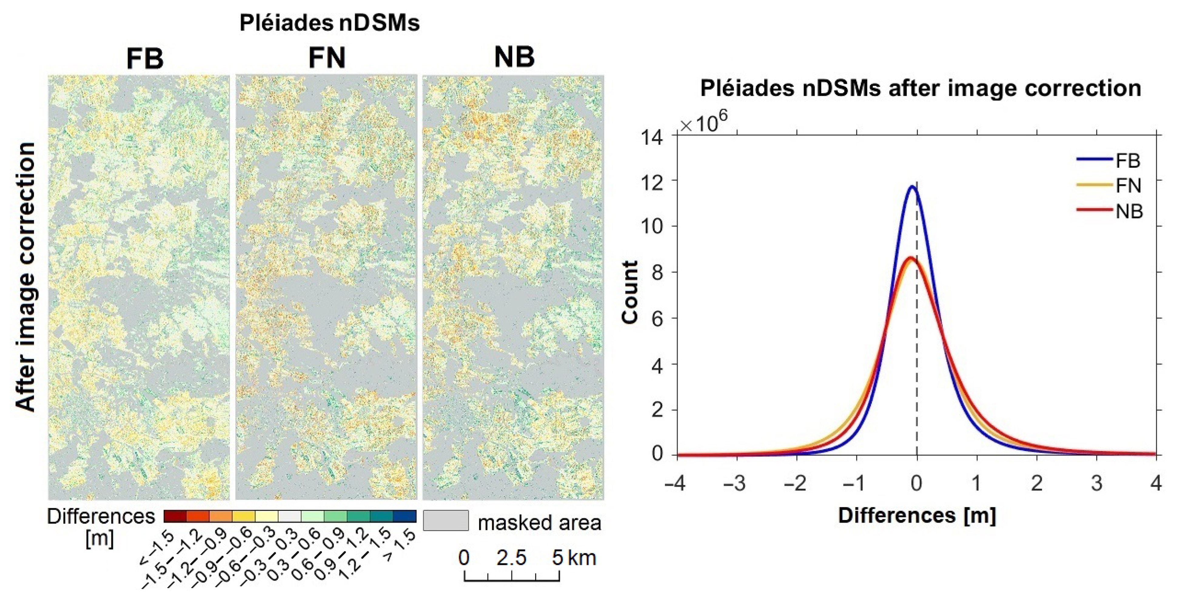
3.3.3. Evaluation of Pléiades DSMs after Image Geometry Correction
The distortions in the satellite images were corrected by using the warping technique and together with the GCPs were finally used as input in a new photogrammetric processing chain for deriving elevation models.
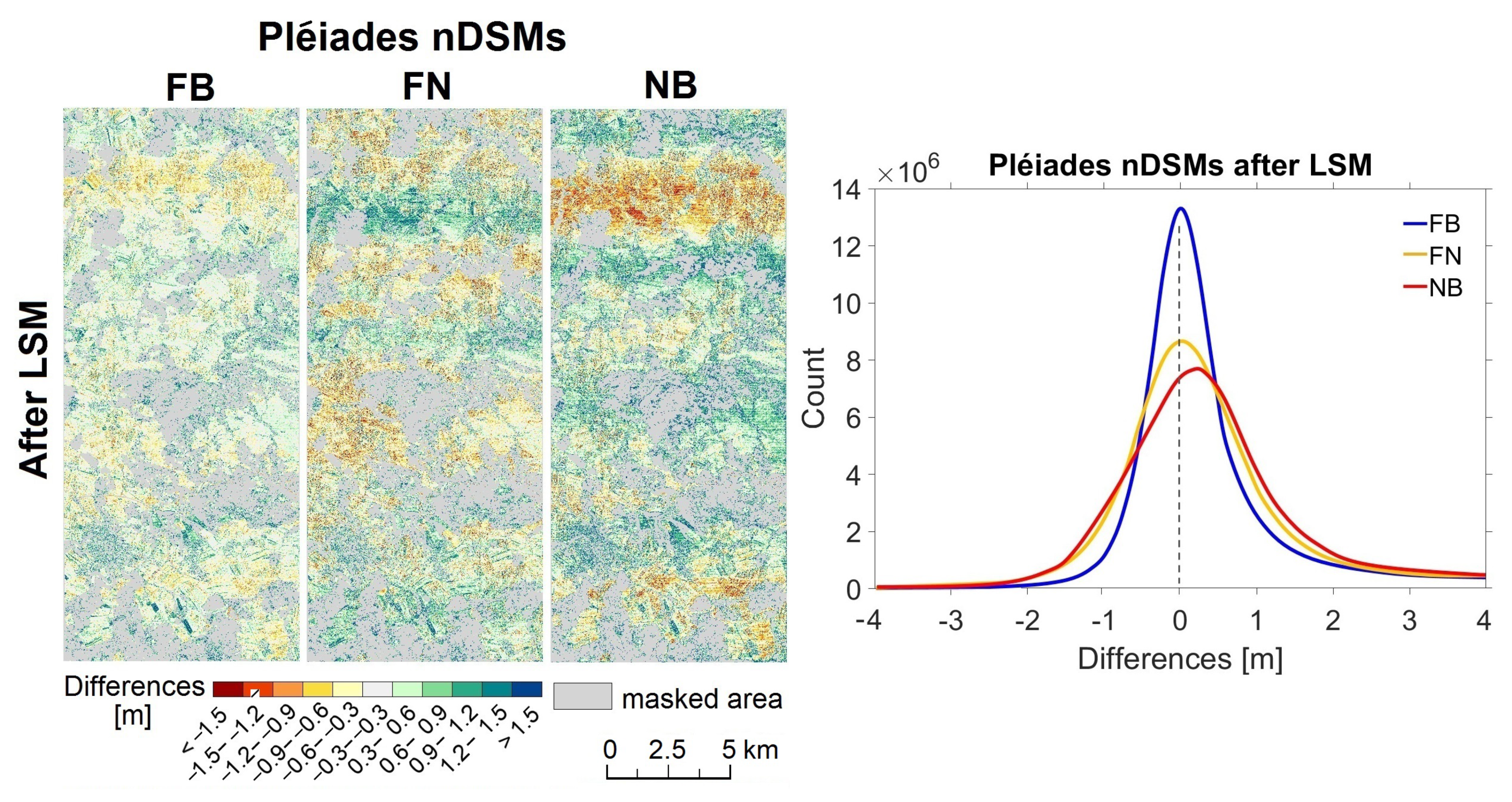
The new interpolated satellite-based DEMs in open, smooth areas for each stereo pair were again compared with the ALS reference model. As visible in Figure 17, the systematic elevation differences (with oscillation pattern) are successfully removed by applying the image correction functions. The section profile in the along-track direction with Z-elevation differences of pairwise DSMs against the reference Lidar DTM shows values close to 0 m after correction (Figure 18). Initially with maximum elevation differences of up to 0.88 m (Figure 14), the improved DSMs show less than 0.10 cm differences after correction.
Table 6 shows the vertical differences statistics of Pléiades-based DSMs before and after applying image distortion correction. Initially systematically shifted (mean values of −0.10 m, −0.32 m and 0.21 m), the difference models are reduced to mean values very close to zero. The image correction approach significantly reduced the RMS values in each scene combination with up to 34%, with highest improvement for the NB scene combination (from 0.85 m to 0.56 m).
4. Discussion
4.1. Suitability of Coarser Resolution DSMs for Satellite Image Geometry Improvement
Our method is developed based on a reference high resolution terrain model from Lidar. However, in order to test the possibility of improving VHR satellite image geometry by using a coarser resolution elevation model, the open source ALOS World 3D (AW3D30) DSM was chosen. As a freely available global dataset with 1" resolution (equivalent to approximately 30 m at the Equator), the AW3D30 elevation model could be considered as appropriate reference data for the vertical accuracy assessment of the photogrammetrically derived satellite models. However, investigations with respect to its own vertical accuracy should be performed. Acquired by the Panchromatic Remote Sensing Instrument for Stereo Mapping (PRISM) operated on the ALOS (“Daichi”), the AW3D30 was photogrammetrically developed by the Japan Aerospace Exploration Agency (JAXA) using optical imagery collected during the mission between 2006 and 2011. The geographic coordinates refer to the GRS80 ellipsoid (ITRF97), while elevations to the EGM96 geoid [62]. In the literature, studies assessing the vertical accuracy of AW3D30 generally report values of approximately 5 m. However, various research papers demonstrate a better performance with errors below 5 m [63,64].
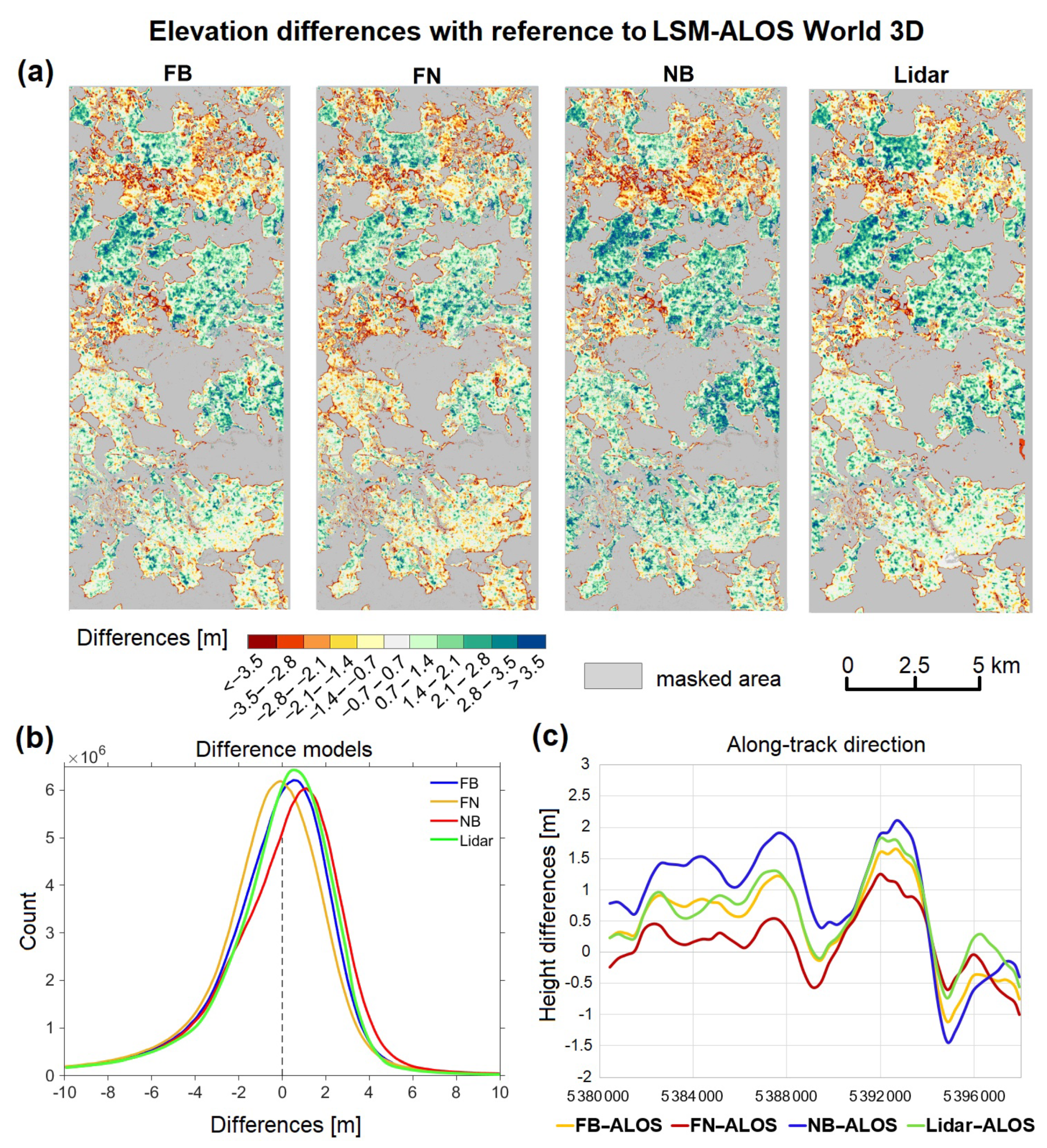
In the current investigation, the vertical quality of the ALOS elevation model was checked against the available Lidar DTM in the Allentsteig study area for the open areas, by computing the statistic parameters and by visual analysis of the colored difference model (Figure 19, Table 7). For this, the AW3D30 model was up-sampled to 1 m resolution, by applying a cubic interpolation. The results indicate an RMSE of 2.79 m with a standard deviation of 2.32 m, values smaller than the accuracies of 4 m and 4.10 m reported in [62,65], respectively.
To check the possibility of using the AW3D30 elevation model as a reference instead of Lidar for image correction model estimation, the difference models between photogrammetric satellite DSMs and AW3D30 were computed. For this, a roughness and elevation mask was computed for removing the vegetation and build-up areas, such that only open, free areas are investigated. The resulting discrepancies are generally high (RMSE up to 3 m) and consequently, the Z elevations section profile in the along-track direction (Figure 19c) shows higher ondulations when compared to the ones determined by using Lidar model as a reference (Figure 17b).
The statistic parameter comparison between the vertical assessments of Pléiades DEMs against Lidar DTM and AW3D30 reveals a lower performance of the AW3D30 DEM with about 2 m in standard deviation and RMSE (Table 7).
To improve the vertical quality of the AW3D30 model, a global LSM approach was employed for estimating a full 3D affine transformation with 12 parameters towards the Lidar reference model. This resulted in rather small improvements (0.17 m), with the RMSE value decreasing from 2.79 m to 2.62 m (Table A1). Nevertheless, the systematic errors are still kept in the Lidar-AW3D30 difference elevation model. Similar to before, the Pléiades DEMs and Lidar were compared against the LSM AW3D30 model in open areas. From a visual inspection, after the global LSM transformation we obtained a better agreement between satellite-based DEMs and the reference AW3D30 (Figure A1). Initially systematically shifted by ≈ 1 m, the Pléiades-based heights were reduced to medians close to zero after applying LSM transformation, with the FB image combination elevation model showing better accuracy then the other two.
Since the RMSE between Pléiades DSMs and AW3D30 is ≈2 m the resulted elevation undulation effects in object space are higher compared to Lidar by a factor of three (from 0.7 m to 2.3 m). Therefore, following a similar workflow for estimating the image corrections based on the AW3D30 model will lead to an overestimation by a factor of three for the correction values in image space. These systematic errors with respect to the Lidar DTM may be caused by instabilities of the ALOS sensor. Consequently the AW3D30 model is not accurate enough for computing the systematic errors in the Pléiades DSMs with amplitudes of maximum 0.88 m.
4.2. Further Remarks
Computed with our proposed method, our resulted image correction values for the tri-stereo Pléiades satellite images (with a maximum amplitude of 0.075 pixels) align very well with the values reported by Jacobsen in [35], where the Pléiades stereo scenes have systematic effects below 0.10 pixels.
The triple stereo scene allows a further verification of the image geometry correction. In Figure 8 the differences between the surface models of the different image pairs before image geometry correction were shown. These pairwise DSM differences after image geometry correction, , , and , are shown in Figure 20. The difference is dominated by random noise and systematic patterns in height are below 14 cm. This shows the effectiveness of the proposed algorithm.
As presented in Table 6, height errors of the FB, FN, and NB error are 44 cm, 57 cm, and 56 cm, respectively, whereas the systematic errors are below 14 cm. Thus, systematic errors are clearly below the random error components. The formula for the precision of heights derived by forward intersection is: [66], with the image scale and the image measurement precision. The base height ratios are given in Table 1. From this, the image measurement precision can be computed for each pair and amounts to 10% to 15% of the pixel size. It has to be considered, however, that the DSM interpolation (Section 2.2) also introduces some smoothing, and these values are too optimistic for the estimation of measurement precision in dense matching. This would explain the better accuracy than reported in [67] for very high resolution aerial photography (GSD < 10 cm), which suggests DSM accuracy between 0.5 GSD and 1 GSD for much more favourable B/H ratios.
Comparative analyses regarding the vertical accuracy assessment have also been conducted on other Pléiades and WorldView-3 DSMs. In these datasets, the same periodic systematic vertical offsets (undulation effects in the flight direction) were visible. This confirms again that attitude sensor oscillations are affecting the satellite imaging geometry, causing distortions that need to be corrected. However, these analyses need to be further investigated. Our results show that not only the investigated Pléiades DSMs suffer from errors, but also the elevation model from ALOS sensor displays periodic height discrepancies when compared against the Lidar DTM reference. This might be caused by the existing distortions in the ALOS prism images, also reported in [44,68].
These findings add further knowledge to the specific topic, by extending the currently existing list of optical sensors with limited orientation accuracies, as formulated by Jacobsen in [69]. His research demonstrates that several optical sensors, among which the Chinese ZiYuan-3, SPOT-5, WorldView-2, and Cartosat, have limited orientation accuracies, a fact that causes deformations in final derived elevation models.
5. Conclusions
In this paper we have proposed an approach for the analysis and estimation of VHR satellite image distortions caused by attitude oscillations in the flight direction, by the use of a stereo triplet with vendor-provided RPCs and a high resolution elevation model. For this purpose, three Pléiades images were tested and the experimental results demonstrated the effectiveness of the proposed method, which improves the satellite image geopositioning accuracy. Additionally, a thorough analysis regarding satellite-based DSMs accuracy analysis is presented and different improvement strategies of the Pléiades DSMs were conducted.
From the performed experiments, the following conclusions can be drawn:
- (1)
- In the flying direction, the geometric accuracy of Pléiades images depends on the sensor attitude, which is apparently affected by satellite oscillations.
- (2)
- When compared to a Lidar high resolution elevation model, the computed satellite-based DSMs show periodic systematic height errors as undulations (similar to waves with a maximum amplitude of 1.5 pixels) visible in the along-track direction. This suggests that image orientations are not sufficiently determined by employing a common number of GCPs for RPC bias-correction.
- (3)
- The periodic vertical offsets in the computed DSMs could not be effectively compensated even if the number of GCPs was increased to 300. This strategy brought improvements to the vertical accuracy of the Pléiades DSMs with 20% in the overall RMSE, which implies that the accuracy in height is sensitive to the number and distribution of GCPs. Nevertheless, the systematic elevation offsets are preserved.
- (4)
- Similar to the 300 GCPs strategy, the applied global LSM technique in object space brought significant improvements to the photogrammetrically derived DSMs, since the RMSE were reduced by 26%. However, the systematics in-track direction are still present.
- (5)
- The preservation of systematic height errors in the computed satellite-based elevation models suggests a not sufficient bias-correction model for the RPCs. This is explained by the fact that in the flying direction, satellite image geometry highly depends on the accuracy of the sensor orientation angle. Hence, a quick change in viewing direction leads to sensor vibrations, which cannot be captured by the bias-compensated 3rd-order rational polynomial coefficients.
- (6)
- The proposed approach based on corrections in image space can detect and estimate the periodic image distortions in-track direction. With amplitudes of less than 0.10 pixels, oscillation period (T) of 0.70 s, and frequency of 1.42 Hz, the image corrections describe actually the small vibrations of the Pléiades satellite during image acquisition with a pitch angle of degrees.
- (7)
- The effectiveness of our method is proven by the successfull removal of the systematic elevations discrepancies in the DSM and by the improvement of the overall accuracy with 33% in RMSE.
Overall, besides DSM quality improvement, our method presents an image post-processing scheme to eliminate the negative influence of the attitude oscillation for geo-positioning. Nevertheless, the proposed approach has two important requirements: a very highly accurate reference model and a landscape which is (at least) partly open. It will not work for areas with complete forest coverage.
The improved satellite-based DSMs can be further used to compute object heights [70] given a high resolution DTM, but also in many forestry applications, for example to detect tree growth [71,72].
In this study, only Pléiades tri-stereo images were tested. More Pléiades images covering different areas, with distinct topography are required to further analyze the influence of satellite attitude oscillations on the accuracy of satellite-based DSMs. Additionally, further studies on other VHR satellite data sets are also necessary to evaluate the performance of the proposed approach. We expect variations from image to image and only the character and size of deformations to be typical for a specific optical satellite, but this also depends upon the operating conditions due to high speed and fast satellite rotation. Although the method was inspired by and applied to VHR satellite images, the application on other dynamically accquired (i.e., scanned) data where oscilating errors may also appear (e.g., from line cameras or laser scanners) seems an interesting future task.
Author Contributions
Conceptualization, A.-M.L., N.P. and J.O.-S.; methodology, A.-M.L., C.R. and J.O.-S.; software, J.O.-S. and C.R.; validation, A.-M.L., N.P., C.R. and J.O.-S.; formal analysis, A.-M.L.; investigation, A.-M.L.; resources, J.O.-S., C.R. and N.P.; Data curation, A.-M.L. and J.O.-S.; writing—original draft preparation, A.-M.L.; writing—review and editing, A.-M.L., N.P., C.R. and J.O.-S.; visualization, A.-M.L.; supervision, N.P., C.R. and J.O.-S.; project administration, N.P. and J.O.-S.; funding acquisition, N.P., J.O.-S. All authors have read and agreed to the published version of the manuscript.
Funding
The work was partly funded by the Austrian Research Promotion Agency (FFG), Vienna, Austria.
Institutional Review Board Statement
Not applicable.
Informed Consent Statement
Not applicable.
Data Availability Statement
Not applicable.
Acknowledgments
The authors acknowledge Open Access Funding by TU Wien. We express our gratitude to the Institüt für Militärisches Geowesen (Wien) for support in satellite image acquisition and the company Vermessung Schmid ZT GmbH for providing the RTK ground control point coordinates used in this investigation.
Conflicts of Interest
The authors declare no conflict of interest.
Abbreviations
The following abbreviations are used in this manuscript:
| VHR | Very High Resolution |
| ALS | Airborne Laser Scanning |
| LiDAR | Light Detection And Ranging |
| DEM | Digital Elevation Model |
| DTM | Digital Terrain Model |
| DSM | Digital Surface Model |
| RFM | Rational Function Model |
| RPC | Rational Polynomial Coefficient |
| GSD | Ground Sampling Distance |
| GCP | Ground Control Point |
| CP | Check Point |
| TP | Tie Point |
| CBM | Cost Based Matching |
| FBM | Feature Based Matching |
| LSM | Least Squares Matching |
| DIM | Dense Image Matching |
| RTK | Real Time Kinematic |
| GNSS | Global Navigation Satellite System |
Appendix A
Figure A1 shows the difference elevation models between pairwise Pléiades DEMs and Lidar with reference to the improved AW3D30 model (by using the LSM technique). Resulting statistics are given in Table A1.

Table A1.
LSM ALOS (after LSM to Lidar) vertical accuracy with reference to Lidar and comparison of Pléiades DEMs with respect to Lidar and LSM ALOS in open areas (given values are in meters).
Table A1.
LSM ALOS (after LSM to Lidar) vertical accuracy with reference to Lidar and comparison of Pléiades DEMs with respect to Lidar and LSM ALOS in open areas (given values are in meters).
| Elevation Models | Lidar Reference | LSM ALOS Reference | ||||||||
|---|---|---|---|---|---|---|---|---|---|---|
| μ | Med | σ | σMAD | RMSE | μ | Med | σ | σMAD | RMSE | |
| LSM ALOS | −0.18 | 0.17 | 2.76 | 2.14 | 2.62 | |||||
| Pléiades comb. | ||||||||||
| FB | −0.10 | −0.16 | 0.64 | 0.53 | 0.65 | −0.27 | 0.04 | 2.70 | 2.21 | 2.71 |
| FN | −0.32 | −0.39 | 0.78 | 0.73 | 0.84 | −0.54 | −0.31 | 2.70 | 2.19 | 2.76 |
| NB | 0.21 | 0.24 | 0.83 | 0.82 | 0.85 | 0.05 | 0.42 | 2.82 | 2.36 | 2.82 |
Figure A1.
Elevation differences (Pléiades DEMs and Lidar DTM) with respect to LSM ALOS World 3D reference: (a) Color coded height difference models (masked areas are shown in grey). (b) Frequency distribution of height discrepancies for all combinations. (c) Section profile in along-track direction with Z elevation differences of pairwise DSMs against reference LSM-ALOS World 3D.

References
- Holland, D.; Boyd, D.; Marshall, P. Updating topographic mapping in Great Britain using imagery from high-resolution satellite sensors. ISPRS J. Photogramm. Remote Sens. 2006, 60, 212–223. [Google Scholar] [CrossRef]
- Nichol, J.E.; Shaker, A.; Wong, M.S. Application of high-resolution stereo satellite images to detailed landslide hazard assessment. Geomorphology 2006, 76, 68–75. [Google Scholar] [CrossRef]
- Poon, J.; Fraser, C.S.; Chunsun, Z.; Li, Z.; Gruen, A. Quality assessment of digital surface models generated from IKONOS imagery. Photogramm. Rec. 2005, 20, 162–171. [Google Scholar] [CrossRef]
- Toutin, T.; Schmitt, C.; Wang, H. Impact of no GCP on elevation extraction from WorldView stereo data. ISPRS J. Photogramm. Remote Sens. 2012, 72, 73–79. [Google Scholar] [CrossRef]
- Tong, X.; Ye, Z.; Xu, Y.; Tang, X.; Liu, S.; Li, L.; Xie, H.; Wang, F.; Li, T.; Hong, Z. Framework of jitter detection and compensation for high resolution satellites. Remote Sens. 2014, 6, 3944–3964. [Google Scholar] [CrossRef] [Green Version]
- Wang, M.; Zhu, Y.; Pan, J.; Yang, B.; Zhu, Q. Satellite jitter detection and compensation using multispectral imagery. Remote Sens. Lett. 2016, 7, 513–522. [Google Scholar] [CrossRef]
- Fraser, C.S.; Dial, G.; Grodecki, J. Sensor orientation via RPCs. ISPRS J. Photogramm. Remote Sens. 2006, 60, 182–194. [Google Scholar] [CrossRef]
- Zhang, Y.; Zheng, M.; Xiong, X.; Xiong, J. Multistrip bundle block adjustment of ZY-3 satellite imagery by rigorous sensor model without ground control point. IEEE Geosci. Remote Sens. Lett. 2014, 12, 865–869. [Google Scholar] [CrossRef]
- Jiang, Y.H.; Zhang, G.; Tang, X.; Li, D.R.; Wang, T.; Huang, W.C.; Li, L.T. Improvement and assessment of the geometric accuracy of Chinese high-resolution optical satellites. IEEE J. Sel. Top. Appl. Earth Obs. Remote Sens. 2015, 8, 4841–4852. [Google Scholar] [CrossRef]
- Oh, J.; Lee, C. Automated bias-compensation of rational polynomial coefficients of high resolution satellite imagery based on topographic maps. ISPRS J. Photogramm. Remote Sens. 2015, 100, 14–22. [Google Scholar] [CrossRef]
- Shen, X.; Li, Q.; Wu, G.; Zhu, J. Bias compensation for rational polynomial coefficients of high-resolution satellite imagery by local polynomial modeling. Remote Sens. 2017, 9, 200. [Google Scholar] [CrossRef] [Green Version]
- Dong, Y.; Lei, R.; Fan, D.; Gu, L.; Ji, S. A novel RPC bias model for improving the positioning accuracy of satellite images. ISPRS Ann. Photogramm. Remote Sens. Spat. Inf. Sci. 2020, 5, 35–41. [Google Scholar] [CrossRef]
- Hu, Y.; Tao, V.; Croitoru, A. Understanding the rational function model: Methods and applications. Int. Arch. Photogramm. Remote Sens. 2004, 20, 119–124. [Google Scholar]
- Poli, D.; Toutin, T. Review of developments in geometric modelling for high resolution satellite pushbroom sensors. Photogramm. Rec. 2012, 27, 58–73. [Google Scholar] [CrossRef]
- Toutin, T. State-of-the-art of geometric correction of remote sensing data: A data fusion perspective. Int. J. Image Data Fusion 2011, 2, 3–35. [Google Scholar] [CrossRef]
- Tong, X.; Liu, S.; Weng, Q. Bias-corrected rational polynomial coefficients for high accuracy geo-positioning of QuickBird stereo imagery. ISPRS J. Photogramm. Remote Sens. 2010, 65, 218–226. [Google Scholar] [CrossRef]
- Dial, G.; Grodecki, J. Block adjustment with rational polynomial camera models. In Proceedings of the ASPRS 2002 Conference, Washington, DC, USA, 19–26 April 2002; pp. 22–26. [Google Scholar]
- Aguilar, M.A.; Aguilar, F.J.; Mar Saldaña, M.d.; Fernández, I. Geopositioning accuracy assessment of GeoEye-1 panchromatic and multispectral imagery. Photogramm. Eng. Remote Sens. 2012, 78, 247–257. [Google Scholar] [CrossRef]
- Alkan, M.; Buyuksalih, G.; Sefercik, U.G.; Jacobsen, K. Geometric accuracy and information content of WorldView-1 images. Opt. Eng. 2013, 52, 026201. [Google Scholar] [CrossRef]
- Fraser, C.S.; Hanley, H.B. Bias-compensated RPCs for sensor orientation of high-resolution satellite imagery. Photogramm. Eng. Remote Sens. 2005, 71, 909–915. [Google Scholar] [CrossRef]
- Tao, C.V.; Hu, Y.; Jiang, W. Photogrammetric exploitation of IKONOS imagery for mapping applications. Int. J. Remote Sens. 2004, 25, 2833–2853. [Google Scholar] [CrossRef]
- Grodecki, J.; Dial, G. IKONOS geometric accuracy validation. Int. Arch. Photogramm. Remote Sens. Spat. Inf. Sci. 2002, 34, 50–55. [Google Scholar]
- Fraser, C.S.; Hanley, H.B. Bias compensation in rational functions for IKONOS satellite imagery. Photogramm. Eng. Remote Sens. 2003, 69, 53–57. [Google Scholar] [CrossRef]
- Noguchi, M.; Fraser, C.S.; Nakamura, T.; Shimono, T.; Oki, S. Accuracy assessment of QuickBird stereo imagery. Photogramm. Rec. 2004, 19, 128–137. [Google Scholar] [CrossRef]
- Teo, T.A. Bias compensation in a rigorous sensor model and rational function model for high-resolution satellite images. Photogramm. Eng. Remote Sens. 2011, 77, 1211–1220. [Google Scholar] [CrossRef]
- Shen, X.; Liu, B.; Li, Q.Q. Correcting bias in the rational polynomial coefficients of satellite imagery using thin-plate smoothing splines. ISPRS J. Photogramm. Remote Sens. 2017, 125, 125–131. [Google Scholar] [CrossRef]
- Hong, Z.; Tong, X.; Liu, S.; Chen, P.; Xie, H.; Jin, Y. A comparison of the performance of bias-corrected RSMs and RFMs for the geo-positioning of high-resolution satellite stereo imagery. Remote Sens. 2015, 7, 16815–16830. [Google Scholar] [CrossRef] [Green Version]
- Grodecki, J.; Dial, G. Block adjustment of high-resolution satellite images described by rational polynomials. Photogramm. Eng. Remote Sens. 2003, 69, 59–68. [Google Scholar] [CrossRef]
- Zhang, Y.; Lu, Y.; Wang, L.; Huang, X. A new approach on optimization of the rational function model of high-resolution satellite imagery. IEEE Trans. Geosci. Remote Sens. 2011, 50, 2758–2764. [Google Scholar] [CrossRef]
- Aguilar, M.A.; del Mar Saldana, M.; Aguilar, F.J. Assessing geometric accuracy of the orthorectification process from GeoEye-1 and WorldView-2 panchromatic images. Int. J. Appl. Earth Obs. Geoinf. 2013, 21, 427–435. [Google Scholar] [CrossRef]
- Cao, J.; Fu, J.; Yuan, X.; Gong, J. Nonlinear bias compensation of ZiYuan-3 satellite imagery with cubic splines. ISPRS J. Photogramm. Remote Sens. 2017, 133, 174–185. [Google Scholar] [CrossRef]
- Jacobsen, K. Satellite image orientation. Int. Arch. Photogramm. Remote Sens. Spat. Inf. Sci. 2008, 37, 703–709. [Google Scholar]
- Kornus, W.; Lehner, M.; Schroeder, M. Geometric inflight-calibration by block adjustment using MOMS-2P-imagery of three intersecting stereo-strips. In Proceedings of the ISPRS Workshop on Sensors and Mapping from Space, Hannover, Germany, 27–30 September 1999; pp. 27–30. [Google Scholar]
- Dial, G.; Grodecki, J. Test ranges for metric calibration and validation of high-resolution satellite imaging systems. In Post-Launch Calibration of Satellite Sensors, Proceedings of the International Workshop on Radiometric and Geometric Calibration, Gulfport, MI, USA, 2–5 December 2003; CRC Press: Boca Raton, FL, USA, 2004; Volume 2, p. 171. [Google Scholar]
- Jacobsen, K. Systematic geometric image errors of very high resolution optical satellites. Int. Arch. Photogramm. Remote Sens. Spat. Inf. Sci. 2018, 42, 233–238. [Google Scholar] [CrossRef] [Green Version]
- Pan, J.; Che, C.; Zhu, Y.; Wang, M. Satellite jitter estimation and validation using parallax images. Sensors 2017, 17, 83. [Google Scholar] [CrossRef] [PubMed] [Green Version]
- Teshima, Y.; Iwasaki, A. Correction of attitude fluctuation of Terra spacecraft using ASTER/SWIR imagery with parallax observation. IEEE Trans. Geosci. Remote Sens. 2007, 46, 222–227. [Google Scholar] [CrossRef]
- Amberg, V.; Dechoz, C.; Bernard, L.; Greslou, D.; De Lussy, F.; Lebegue, L. In-flight attitude perturbances estimation: Application to PLEIADES-HR satellites. In Earth Observing Systems XVIII; SPIE: Bellingham, WA, USA, 2013; Volume 8866, pp. 327–335. [Google Scholar]
- Tong, X.; Li, L.; Liu, S.; Xu, Y.; Ye, Z.; Jin, Y.; Wang, F.; Xie, H. Detection and estimation of ZY-3 three-line array image distortions caused by attitude oscillation. ISPRS J. Photogramm. Remote Sens. 2015, 101, 291–309. [Google Scholar] [CrossRef]
- Ayoub, F.; Leprince, S.; Binet, R.; Lewis, K.W.; Aharonson, O.; Avouac, J.P. Influence of camera distortions on satellite image registration and change detection applications. In Proceedings of the IGARSS 2008-2008 IEEE International Geoscience and Remote Sensing Symposium, Boston, MA, USA, 8–11 July 2008; Volume 2, p. II-1072. [Google Scholar]
- Mattson, S.; Robinson, M.; McEwen, A.; Bartels, A.; Bowman-Cisneros, E.; Li, R.; Lawver, J.; Tran, T.; Paris, K.; Team, L. Early assessment of spacecraft jitter in LROC-NAC. In Proceedings of the 41st Annual Lunar and Planetary Science Conference, The Woodlands, TX, USA, 1–5 March 2010; Volume 41, p. 1871. [Google Scholar]
- Pan, H.; Zhang, G.; Tang, X.; Li, D.; Zhu, X.; Zhou, P.; Jiang, Y. Basic products of the ZiYuan-3 satellite and accuracy evaluation. Photogramm. Eng. Remote Sens. 2013, 79, 1131–1145. [Google Scholar] [CrossRef]
- Robertson, B.C. Rigorous geometric modeling and correction of QuickBird imagery. In Proceedings of the 2003 IEEE International Geoscience and Remote Sensing Symposium (IEEE Cat. No. 03CH37477), Toulouse, France, 21–25 July 2003; Volume 2, pp. 797–802. [Google Scholar]
- Schwind, P.; Schneider, M.; Palubinskas, G.; Storch, T.; Muller, R.; Richter, R. Processors for ALOS optical data: Deconvolution, DEM generation, orthorectification, and atmospheric correction. IEEE Trans. Geosci. Remote Sens. 2009, 47, 4074–4082. [Google Scholar] [CrossRef]
- Mattson, S.; Boyd, A.; Kirk, R.; Cook, D.; Howington-Kraus, E. HiJACK: Correcting spacecraft jitter in HiRISE images of Mars. Health Manag. Technol 2009, 33, A162. [Google Scholar]
- Iwasaki, A. Detection and estimation satellite attitude jitter using remote sensing imagery. Adv. Spacecr. Technol. 2011, 13, 257–272. [Google Scholar]
- Mumtaz, R.; Palmer, P. Attitude determination by exploiting geometric distortions in stereo images of DMC camera. IEEE Trans. Aerosp. Electron. Syst. 2013, 49, 1601–1625. [Google Scholar] [CrossRef]
- Jiang, Y.h.; Zhang, G.; Tang, X.; Li, D.; Huang, W.c. Detection and correction of relative attitude errors for ZY1-02C. IEEE Trans. Geosci. Remote Sens. 2014, 52, 7674–7683. [Google Scholar] [CrossRef]
- Lehner, M.; Müller, R. Quality check of MOMS-2P ortho-images of semi-arid landscapes. In Proceedings of the ISPRS Workshop High Resolution Mapping Space, Hanover, Germany, 6–8 October 2003; pp. 1–5. [Google Scholar]
- Li, R.; Hwangbo, J.; Chen, Y.; Di, K. Rigorous photogrammetric processing of HiRISE stereo imagery for Mars topographic mapping. IEEE Trans. Geosci. Remote Sens. 2011, 49, 2558–2572. [Google Scholar]
- Bostelmann, J.; Heipke, C. Modeling spacecraft oscillations in HRSC images of Mars Express. Int. Arch. Photogramm. Remote Sens. Spat. Inf. Sci. 2011, 38, 51–56. [Google Scholar] [CrossRef] [Green Version]
- Gwinner, K.; Scholten, F.; Preusker, F.; Elgner, S.; Roatsch, T.; Spiegel, M.; Schmidt, R.; Oberst, J.; Jaumann, R.; Heipke, C. Topography of Mars from global mapping by HRSC high-resolution digital terrain models and orthoimages: Characteristics and performance. Earth Planet. Sci. Lett. 2010, 294, 506–519. [Google Scholar] [CrossRef]
- Astrium. Pléiades Imagery—User Guide v 2.0; Technical report; Astrium GEO-Information Services: Toulouse, France, 2012. [Google Scholar]
- Heipke, C. Automation of interior, relative, and absolute orientation. ISPRS J. Photogramm. Remote Sens. 1997, 52, 1–19. [Google Scholar] [CrossRef]
- Toutin, T. Geometric processing of remote sensing images: Models, algorithms and methods. Int. J. Remote Sens. 2004, 25, 1893–1924. [Google Scholar] [CrossRef]
- Förstner, W. Quality assessment of object location and point transfer using digital image correlation techniques. IBID 1984, 25, 197–219. [Google Scholar]
- Maas, H.G. Least-squares matching with airborne laserscanning data in a TIN structure. Int. Arch. Photogramm. Remote Sens. 2000, 33, 548–555. [Google Scholar]
- Ressl, C.; Kager, H.; Mandlburger, G. Quality checking of ALS projects using statistics of strip differences. Int. Arch. Photogramm. Remote Sens. 2008, 37, 253–260. [Google Scholar]
- Ressl, C.; Pfeifer, N.; Mandlburger, G. Applying 3-D affine transformation and least squares matching for airborne laser scanning strips adjustment without GNSS/IMU trajectory Data. In Proceedings of the ISPRS Workshop Laser Scanning, Calgary, AB, USA, 29–31 August 2011. [Google Scholar]
- Piltz, B.; Bayer, S.; Poznanska, A.M. Volume based DTM generation from very high resolution photogrammetric DSMs. Int. Arch. Photogramm. Remote Sens. Spat. Inf. Sci. 2016, 41, 83–90. [Google Scholar] [CrossRef] [Green Version]
- Pfeifer, N.; Mandlburger, G.; Otepka, J.; Karel, W. OPALS–A framework for Airborne Laser Scanning data analysis. Comput. Environ. Urban Syst. 2014, 45, 125–136. [Google Scholar] [CrossRef]
- Tadono, T.; Takaku, J.; Tsutsui, K.; Oda, F.; Nagai, H. Status of “ALOS World 3D (AW3D)” global DSM generation. In Proceedings of the 2015 IEEE International Geoscience and Remote Sensing Symposium (IGARSS), Milan, Italy, 26–31 July 2015; pp. 3822–3825. [Google Scholar]
- Santillan, J.R.; Makinano-Santillan, M.; Makinano, R.M. Vertical accuracy assessment of ALOS World 3D-30M Digital Elevation Model over northeastern Mindanao, Philippines. In Proceedings of the 2016 IEEE International Geoscience and Remote Sensing Symposium (IGARSS), Beijing, China, 10–15 July 2016; pp. 5374–5377. [Google Scholar]
- Caglar, B.; Becek, K.; Mekik, C.; Ozendi, M. On the vertical accuracy of the ALOS world 3D-30m digital elevation model. Remote Sens. Lett. 2018, 9, 607–615. [Google Scholar] [CrossRef]
- Takaku, J.; Tadono, T.; Tsutsui, K. Generation of High Resolution Global DSM from ALOS PRISM. ISPRS Ann. Photogramm. Remote Sens. Spat. Inf. Sci. 2014, 2, 243–248. [Google Scholar] [CrossRef] [Green Version]
- Kraus, K. Photogrammetrie: Geometrische Informationen aus Photographien und Laserscanneraufnahmen; Walter de Gruyter: Berlin, Germany, 2012. [Google Scholar]
- Ressl, C.; Brockmann, H.; Mandlburger, G.; Pfeifer, N. Dense Image Matching vs. Airborne Laser Scanning–Comparison of two methods for deriving terrain models. Photogramm. Fernerkund. Geoinf. 2016, 57–73. [Google Scholar] [CrossRef]
- Takaku, J.; Tadono, T. High resolution dsm generation from alos prism-processing status and influence of attitude fluctuation. In Proceedings of the 2010 IEEE International Geoscience and Remote Sensing Symposium, Honolulu, HI, USA, 25–30 July 2010; pp. 4228–4231. [Google Scholar]
- Jacobsen, K. Verbesserung der Geometrie von Satellitenbildern durch Höhenmodelle. In Publikationen der Deutschen Gesellschaft für Photogrammetrie; Würzburg, Germany, 2017; p. 13. [Google Scholar]
- Loghin, A.M.; Otepka-Schremmer, J.; Pfeifer, N. Potential of Pléiades and WorldView-3 tri-stereo DSMs to represent heights of small isolated objects. Sensors 2020, 20, 2695. [Google Scholar] [CrossRef]
- Piermattei, L.; Marty, M.; Karel, W.; Ressl, C.; Hollaus, M.; Ginzler, C.; Pfeifer, N. Impact of the acquisition geometry of very high-resolution Pléiades imagery on the accuracy of canopy height models over forested alpine regions. Remote Sens. 2018, 10, 1542. [Google Scholar] [CrossRef] [Green Version]
- Piermattei, L.; Marty, M.; Ginzler, C.; Pöchtrager, M.; Karel, W.; Ressl, C.; Pfeifer, N.; Hollaus, M. Pléiades satellite images for deriving forest metrics in the Alpine region. Int. J. Appl. Earth Obs. Geoinf. 2019, 80, 240–256. [Google Scholar] [CrossRef]
Figure 1.
Processing workflow for satellite image geometry correction model.

Figure 2.
Satellite image acquisition for the study area: (a) Overview map of Austria with marked location of the study area (coordinates in UTM zone 33N). (b) Pléiades tri-stereo acquisition geometry (view of satellite positions in Google Earth). (c) Acquisition footprint visualized in Google Earth.

Figure 3.
Measurement of GCPs: (a) GCPs measured by means of RTK GNSS (left column) and manually measured in orthophoto (right column). (b) Overview of GCPs’ distribution in Google Earth.
Figure 3.
Measurement of GCPs: (a) GCPs measured by means of RTK GNSS (left column) and manually measured in orthophoto (right column). (b) Overview of GCPs’ distribution in Google Earth.

Figure 4.
Overview of the 300 manually measured GCPs’ distribution in Match-AT software.

Figure 5.
Definition of 3D point profile-lines at 10 m intervals.

Figure 6.
Computation of image corrections.

Figure 7.
Differences between Pléiades and Lidar reference DTM in open areas: (a) Color-coded height differences (masked areas are shown in grey). (b) Frequency distribution of height discrepancies. (c) Section profile in along-track direction with Z elevation differences.
Figure 7.
Differences between Pléiades and Lidar reference DTM in open areas: (a) Color-coded height differences (masked areas are shown in grey). (b) Frequency distribution of height discrepancies. (c) Section profile in along-track direction with Z elevation differences.

Figure 8.
Differences between Pléiades pairwise DSMs: (a) Color-coded height differences. (b) Frequency distribution of height discrepancies. (c) Section profile in along-track direction with Z elevation differences.
Figure 8.
Differences between Pléiades pairwise DSMs: (a) Color-coded height differences. (b) Frequency distribution of height discrepancies. (c) Section profile in along-track direction with Z elevation differences.

Figure 9.
Image re-projection errors of the 43 GCPs and 373 TPs in the Allentsteig dataset based on bias-corrected RPC orientation. Overview of scaled image residuals in Forward, Nadir and Backward images. The vectors were exaggerated 5000 times to enable better illustration.
Figure 9.
Image re-projection errors of the 43 GCPs and 373 TPs in the Allentsteig dataset based on bias-corrected RPC orientation. Overview of scaled image residuals in Forward, Nadir and Backward images. The vectors were exaggerated 5000 times to enable better illustration.

Figure 10.
Image re-projection errors of the 300 GCPs in the Allentsteig dataset based on bias-corrected RPC orientation: (a) Overview of scaled image residuals in Forward, Nadir and Backward images with marked 8 and 20 section divisions in the flight direction. The vectors were exaggerated 5000 times to enable better illustration. (b) Median of y residuals with corresponding robust standard deviations for 8 along-track intervals. (c) Median of y residuals with corresponding robust standard deviations for 20 along-track intervals.

Figure 11.
Differences between GCPs’ coordinates from terrain measurement to reconstruction from oriented satellite images: (a) Coordinate differences. (b) Statistics on GCPs’ coordinates and on elevations in open areas.
Figure 11.
Differences between GCPs’ coordinates from terrain measurement to reconstruction from oriented satellite images: (a) Coordinate differences. (b) Statistics on GCPs’ coordinates and on elevations in open areas.

Figure 12.
Pléiades nDSMs for open areas with corresponding frequency distribution of height discrepancies: (a) Image georeferencing with bias-corrected RPCs using 43 GCPs. (b) Image georeferencing with bias-corrected RPCs using 300 GCPs.
Figure 12.
Pléiades nDSMs for open areas with corresponding frequency distribution of height discrepancies: (a) Image georeferencing with bias-corrected RPCs using 43 GCPs. (b) Image georeferencing with bias-corrected RPCs using 300 GCPs.

Figure 13.
Pléiades nDSMs (RPC refinement with 43 GCPs) for open areas after global LSM. Color-coded height differences (masked areas are shown in grey) with corresponding frequency distribution of height discrepancies for all combinations (to be compared with Pléiades nDSMs before global LSM in Figure 12a).

Figure 14.
Elevation corrections shown as profile-height differences for pairwise Pléiades nDSMs.

Figure 15.
Correction functions for Pléiades satellite imagery: (a) Forward image. (b) Nadir image. (c) Backward image. (d) Averaged values.
Figure 15.
Correction functions for Pléiades satellite imagery: (a) Forward image. (b) Nadir image. (c) Backward image. (d) Averaged values.

Figure 16.
Histograms of correction values for Pléiades satellite imagery: (a) Forward image. (b) Nadir image. (c) Backward image.
Figure 16.
Histograms of correction values for Pléiades satellite imagery: (a) Forward image. (b) Nadir image. (c) Backward image.

Figure 17.
Pléiades nDSMs for open areas after image correction (RPC refinement with 300 GCPs). Color-coded height differences (masked areas are shown in grey) with corresponding frequency distribution of height discrepancies of Pléiades DSMs against reference Lidar DTM (to be compared with Pléiades nDSMs before image correction in Figure 12b).

Figure 18.
Section profile in the along-track direction with Z elevation differences of pairwise DSMs against the reference Lidar DTM before (square-dot lines) and after (solid lines) image geometry correction (to be compared with elevation corrections in Figure 14).
Figure 18.
Section profile in the along-track direction with Z elevation differences of pairwise DSMs against the reference Lidar DTM before (square-dot lines) and after (solid lines) image geometry correction (to be compared with elevation corrections in Figure 14).

Figure 19.
Elevation differences (Pléiades DEMs and Lidar DTM) with respect to ALOS World 3D reference: (a) Color coded height difference models (masked areas are shown in grey). (b) Frequency distribution of height discrepancies for all combinations. (c) Section profile in the along-track direction with Z elevation differences of pairwise DSMs against the reference ALOS World 3D.

Figure 20.
Differences between Pléiades pairwise DSMs after image geometry correction: (a) Color-coded height differences. (b) Frequency distribution of height discrepancies. (c) Section profile in the along-track direction with Z elevation differences before (square-dot lines) and after (solid lines) image geometry correction (to be compared with Figure 8).

Table 1.
Acquisition properties for the tri-stereo satellite image dataset over Allentsteig.
| Acq. Date | Acq. Time (UTC) | Image (View) | GSD [m] | Viewing Angles [°] | B/H Ratio | Convergence Angle (°) | |
|---|---|---|---|---|---|---|---|
| In-Track | Cross-Track | ||||||
| 13 June 2017 | 10:09:51.5 | Forward | 0.71 | 3.15 | −5.66 | 0.13 (FN) | 7.5 (FN) |
| 10:10:03.7 | Nadir | 0.70 | 3.37 | 0.46 | 0.11 (NB) | 6.3 (NB) | |
| 10:10:14.0 | Backward | 0.71 | 3.62 | 5.19 | 0.24 (FB) | 13.8 (FB) | |
Table 2.
Pléiades tri-stereo satellite imagery aerial triangulation results.
| Image | No. GCPs | No. TPs/ Image | Sigma (px) | Image Residual Statistics for GCPs & TP Observations | |||||
|---|---|---|---|---|---|---|---|---|---|
| x-Residual (px) | y-Residual (px) | ||||||||
| μ | σMAD | RMSE | μ | σMAD | RMSE | ||||
| Forward | 373 | 0.00 | 0.26 | 0.26 | 0.00 | 0.13 | 0.13 | ||
| Nadir | 43 | 378 | 0.28 | 0.00 | 0.28 | 0.27 | 0.00 | 0.21 | 0.22 |
| Backward | 375 | 0.00 | 0.26 | 0.26 | 0.00 | 0.12 | 0.12 | ||
| Forward | - | 0.00 | 0.26 | 0.26 | 0.00 | 0.24 | 0.24 | ||
| Nadir | 300 | - | 0.32 | 0.00 | 0.40 | 0.40 | 0.00 | 0.38 | 0.38 |
| Backward | - | 0.00 | 0.32 | 0.31 | 0.00 | 0.32 | 0.31 | ||
Table 3.
Accuracy statistics at 43 GCPs’ coordinates and on elevation for open areas (* Vertical accuracy of Pléiades DSM against Lidar DTM in open, object-free areas).
Table 3.
Accuracy statistics at 43 GCPs’ coordinates and on elevation for open areas (* Vertical accuracy of Pléiades DSM against Lidar DTM in open, object-free areas).
| Study Site | Allentsteig | |||
|---|---|---|---|---|
| Mean (m) | Median (m) | σ (m) | RMSE (m) | |
| Easting | −0.01 | 0.02 | 0.29 | 0.32 |
| Northing | −0.02 | 0.01 | 0.22 | 0.27 |
| Elevation | 0.05 | −0.01 | 0.12 | 0.57 |
| 3D | 0.64 | 0.64 | 0.16 | 0.71 |
| * Open areas (Elevation) | 0.80 | 0.79 | 0.53 | 0.89 |
Table 4.
Accuracy assessment of Pléiades DSMs in open areas (given values are in meters).
| Scene Comb. | RPC Refinement with 43 GCPs | RPC Refinement with 300 GCPs | ||||||
|---|---|---|---|---|---|---|---|---|
| Mean | Std | σMAD | RMSE | Mean | Std | σMAD | RMSE | |
| FB | 0.77 | 0.53 | 0.51 | 0.93 | −0.10 | 0.64 | 0.53 | 0.65 |
| FN | 0.72 | 0.65 | 0.68 | 0.97 | −0.32 | 0.78 | 0.73 | 0.84 |
| NB | 0.78 | 0.70 | 0.73 | 1.04 | 0.21 | 0.83 | 0.82 | 0.85 |
Table 5.
Accuracy assessment (RPC refinement with 43 GCPs) of Pléiades DSMs in open areas (given values are in meters).
Table 5.
Accuracy assessment (RPC refinement with 43 GCPs) of Pléiades DSMs in open areas (given values are in meters).
| Scene Comb. | Before LSM | After LSM | ||||||
|---|---|---|---|---|---|---|---|---|
| Mean | Std | σMAD | RMSE | Mean | Std | σMAD | RMSE | |
| FB | 0.77 | 0.53 | 0.51 | 0.93 | 0.13 | 0.60 | 0.50 | 0.60 |
| FN | 0.72 | 0.65 | 0.68 | 0.97 | 0.13 | 0.75 | 0.72 | 0.76 |
| NB | 0.78 | 0.70 | 0.73 | 1.04 | 0.17 | 0.79 | 0.80 | 0.81 |
Table 6.
Accuracy assessment of Pléiades DSMs in open areas before and after image correction (RPC refinement with 300 GCPs; given values are in meters).
Table 6.
Accuracy assessment of Pléiades DSMs in open areas before and after image correction (RPC refinement with 300 GCPs; given values are in meters).
| Scene Comb. | Before Image Correction | After Image Correction | ||||||
|---|---|---|---|---|---|---|---|---|
| Mean | Std | σMAD | RMSE | Mean | Std | σMAD | RMSE | |
| FB | −0.10 | 0.64 | 0.53 | 0.65 | −0.00 | 0.44 | 0.45 | 0.44 |
| FN | −0.32 | 0.78 | 0.73 | 0.84 | −0.02 | 0.57 | 0.52 | 0.57 |
| NB | 0.21 | 0.83 | 0.82 | 0.85 | 0.10 | 0.55 | 0.51 | 0.56 |
Table 7.
ALOS vertical accuracy with reference to Lidar and comparison of Pléiades DEMs with respect to Lidar and ALOS in open areas (given values are in meters).
Table 7.
ALOS vertical accuracy with reference to Lidar and comparison of Pléiades DEMs with respect to Lidar and ALOS in open areas (given values are in meters).
| Elevation Models | Lidar Reference | ALOS Reference | ||||||||
|---|---|---|---|---|---|---|---|---|---|---|
| μ | Med | σ | σMAD | RMSE | μ | Med | σ | σMAD | RMSE | |
| ALOS | 0.39 | 0.83 | 2.77 | 2.32 | 2.79 | |||||
| Pléiades comb. | ||||||||||
| FB | −0.10 | −0.16 | 0.64 | 0.53 | 0.65 | 0.28 | 0.70 | 2.85 | 2.38 | 2.86 |
| FN | −0.32 | −0.39 | 0.78 | 0.73 | 0.84 | 0.03 | 0.34 | 2.81 | 2.32 | 2.82 |
| NB | 0.21 | 0.24 | 0.83 | 0.82 | 0.85 | 0.62 | 1.08 | 2.98 | 2.54 | 3.04 |
Publisher’s Note: MDPI stays neutral with regard to jurisdictional claims in published maps and institutional affiliations. |
© 2022 by the authors. Licensee MDPI, Basel, Switzerland. This article is an open access article distributed under the terms and conditions of the Creative Commons Attribution (CC BY) license (https://creativecommons.org/licenses/by/4.0/).
Share and Cite
MDPI and ACS Style
Loghin, A.-M.; Otepka-Schremmer, J.; Ressl, C.; Pfeifer, N. Improvement of VHR Satellite Image Geometry with High Resolution Elevation Models. Remote Sens. 2022, 14, 2303. https://doi.org/10.3390/rs14102303
AMA Style
Loghin A-M, Otepka-Schremmer J, Ressl C, Pfeifer N. Improvement of VHR Satellite Image Geometry with High Resolution Elevation Models. Remote Sensing. 2022; 14(10):2303. https://doi.org/10.3390/rs14102303
Chicago/Turabian StyleLoghin, Ana-Maria, Johannes Otepka-Schremmer, Camillo Ressl, and Norbert Pfeifer. 2022. "Improvement of VHR Satellite Image Geometry with High Resolution Elevation Models" Remote Sensing 14, no. 10: 2303. https://doi.org/10.3390/rs14102303
Note that from the first issue of 2016, this journal uses article numbers instead of page numbers. See further details here.