Technical Note

Modeling Post-Sunset Equatorial Spread-F Occurrence as a Function of Evening Upward Plasma Drift Using Logistic Regression, Deduced from Ionosondes in Southeast Asia

by
Prayitno Abadi
1,2,*,
Umar Ali Ahmad
2,
Yuichi Otsuka
3,
Punyawi Jamjareegulgarn
4,
Dyah Rahayu Martiningrum
1,
Agri Faturahman
5,
Septi Perwitasari
6,
Randy Erfa Saputra
2 and
Reza Rendian Septiawan
2
1
Research Center for Climate and Atmosphere, Indonesian National Research and Innovation Agency (BRIN), Bandung 40173, Indonesia
2
School of Electrical Engineering, Telkom University, Kab. Bandung 40257, Indonesia
3
Institute for Space-Earth Environmental Research (ISEE), Nagoya University, Nagoya 464-8601, Japan
4
Space Technology Department Center, King Mongkut’s Institute Technology Ladkrabang (KMITL), Prince of Chumphon Campus, Chumphon 86160, Thailand
5
Research Center for Space, Indonesian National Research and Innovation Agency (BRIN), Bandung 40173, Indonesia
6
National Institute of Information and Communications Technology (NICT), Tokyo 184-8795, Japan
*
Author to whom correspondence should be addressed.
Remote Sens. 2022, 14(8), 1896; https://doi.org/10.3390/rs14081896
Submission received: 26 February 2022 / Revised: 9 April 2022 / Accepted: 11 April 2022 / Published: 14 April 2022

Abstract

:
The occurrence of post-sunset equatorial spread-F (ESF) could have detrimental effects on trans-ionospheric radio wave propagation used in modern communications systems. This problem calls for a simple but robust model that accurately predicts the occurrence of post-sunset ESF. Logistic regression was implemented to model the daily occurrence of post-sunset ESF as a function of the evening upward plasma drift (v). The use of logistic regression is formalized by y ^ = 1 / [ 1 + exp ( z ) ] , where y ^ represents the probability of post-sunset ESF occurrence, and z is a linear function containing v . The value of v is derived from the vertical motion of the bottom side of the F-region in the evening equatorial ionosphere, which is observed by the ionosondes in Southeast Asia. Data points (938) of v and post-sunset ESF occurrence were collected in the equinox seasons from 2003 to 2016. The training set used 70% of the dataset to derive z and y ^ and the remaining 30% was used to test the performance of y ^ . The expression z = 2.25 + 0.14 v was obtained from the training set, and y ^ 0.5 (v ≥ ~16.1 m/s) and y ^ < 0.5 (v < ~16.1 m/s) represented the occurrence and non-occurrence of ESF, respectively, with an accuracy of ~0.8 and a true skill score (TSS) of ~0.6. Similarly, in the testing set, y ^ shows an accuracy of ~0.8 and a TSS of ~0.6. Further analysis suggested that the performance of the z-function can be reliable in the daily F10.7 levels ranging from 60 to 140 solar flux units. The z-function implemented in the logistic regression ( y ^ ) found in this study is a novel technique to predict the post-sunset ESF occurrence. The performance consistency between the training set and the testing set concludes that the z-function and the y ^ values of the proposed model could be a simple and robust mathematical model for daily nowcasting the occurrence or non-occurrence of post-sunset ESFs.

1. Introduction

Historically, equatorial spread-F or ESF refers to the phenomenon of spreading echoes characterizing the F region trace of ionograms recorded by the ionosondes in the equatorial zone, especially during nighttime. The ESF demonstrates the existence of irregularities (plasma density fluctuations) in the F region ionosphere [1]. The research progress in understanding the spatial and temporal variations of ESF occurrence is currently carried out by the coordinated ground-based and spaceborne observations, see [2,3,4,5]. Nowadays, the prediction of ESF occurrence has become an important task in space weather services because the irregularities at the base of the ESF occurrence have disadvantageous effects on trans-ionospheric radio wave propagation in modern communications and navigation systems [6]. In particular, ESF occurrence during the post-sunset period is well-known to be a main cause of scintillation (rapid fluctuation) on L-band signals used in global navigation satellite systems (GNSS) [7] and strong scintillation can cause deep GNSS signal fading [8]. The day-to-day variability in post-sunset ESF occurrence remains challenging, but scientists have attempted to investigate the factors that control the generation of post-sunset ESFs [9]. Hence, developing a simpler and more robust model for nowcasting post-sunset ESFs is necessary for space weather services.
Previous modeling of daily ESF occurrence employed the physics-based models, e.g., using the thermosphere ionosphere electrodynamics general circulation model (TIEGCM) [10] and ground-to-topside model of atmosphere and ionosphere for aeronomy (GAIA) [11]. The physical models, such as TIEGCM and GAIA, have a high complexity of the algorithm in generating the outputs. Furthermore, the outputs from such physical models are not directly the probability of ESF occurrence. Nevertheless, further investigations into the relationship between the outputs from the physical models and real observation of ESF occurrence are needed. In this study, we sought to build a simple model for nowcasting post-sunset ESFs that could potentially be used in space weather services. This model can be defined as an effort to forecast the occurrence of ESF a few hours after sunset by analyzing its controlling factors before and around sunset. The identification and research of the controlling factors of the ESF occurrence were made using previous literature [12,13,14,15]. Moreover, the model also connects the controlling factors to the probability of ESF occurrence. Building a simple mathematical model requires an assumption that the relations among the controlling factors of ESF occurrence are linear functions. Additionally, this model could be beneficial because it can be executed more easily and quickly with lower computational costs to determine the occurrence or non-occurrence of the post-sunset ESF at a certain night.
Based on previous investigations, we identified the prominent factor that controls the probability of post-sunset ESF occurrence daily, namely the daily changes in evening upward plasma drift in the equatorial F region that can be caused by the pre-reversal enhancement (PRE) phenomenon [12,13,14,15]. Importantly, this factor can be measured: evening upward plasma drift can be derived from ionosonde. Additionally, this factor can be used to predict post-sunset ESF occurrence. The proposed simple model of the post-sunset ESF occurrence is a binary classification model; that is, the output of the model is the occurrence or non-occurrence of ESF at certain nights. Therefore, logistic regression is suitable for this type of model.
In this study, we intend to build a mathematical model for the post-sunset ESF occurrence as a function of upward ionospheric plasma drift in the evening equatorial region. It employs logistic regression to build the prediction model of post-sunset ESF occurrence. Using the feature dataset, including the evening upward plasma drift and post-sunset ESF occurrence, we can train the logistic regression model to classify nights with and without post-sunset ESF occurrence. A database of observations from the equatorial ionosondes in Southeast Asia was utilized. In the following sections of this paper, the basic idea of logistic regression for modeling the post-sunset ESF occurrence, data preparation, and the study results have been described. A summary of this study and the extension works have been included.

2. Materials and Methods

2.1. Modeling ESF Occurrence with Logistic Regression

The probability of the post-sunset ESF occurrence must lie between the values 0 and 1, and linear regression cannot be used to deal with this model because the linear model also provides outputs outside the range of 0–1. In contrast, the logistic regression technique can be used to model probability events [16]. The probability of post-sunset ESF occurrence using logistic regression is given by
y ^ = 1 1 + e z
where y ^ represents the probability of ESF occurrence and z is a link function between the controlling factor (or predictor) of the ESF occurrence and the probability of ESF occurrence. As shown in Equation (1), the output of y ^ always ranges between zero and one with any value of z. In this study, we consider only one controlling factor of ESF occurrence, namely the evening upward plasma drift in the equatorial region (hereafter denoted as v). Therefore, the function z contains v. We consider z to be a linear function consisting of v. Mathematically, function z can be expressed as
z = β 0 + β 1 v ,
where β j (j = 0 to 1) are known as regression coefficients.
The regression coefficients ( β j ) in Equation (2) can be estimated by training observational data. Here, we need to train the dataset of v and post-sunset ESF occurrence from observations using the gradient descent technique to obtain the optimum β j . In principle, the gradient descent technique sets the optimum value of β j as a function of z to minimize the errors between the predicted output ( y ^ ) and actual output. The actual output is the occurrence of the post-sunset ESF based on observations that can be either 1 for the occurrence of the post-sunset ESF or 0 for the non-occurrence of the post-sunset ESF. In this study, we used a MATLAB toolbox to execute the gradient descent technique in obtaining the optimum β j in Equation (2). The steps in the gradient descent technique used in this study are briefly described as follows:
1.
Setting the initial value of β j ,
β j t = 0 = [ β 0 t = 0 , β 1 t = 0 ] ,
where t = 0 indicates the initial set of values of β j t = 0 . In this study, we set the initial value of each regression coefficient to zero.
2.
Computing the cost function (error) between the predicted and actual outputs based on logistic regression; hence, the cost function is given by:
J = 1 m [ i = 1 m y i log ( y ^ i ) + ( 1 y i ) log ( 1 y ^ i ) ] ,
where J is the cost function, i represents the number of observation data in the training set ranging from 1 to m (number of observations), y is the actual output of the post-sunset ESF occurrence from the observations, and y ^ is the predicted output of the post-sunset ESF occurrence obtained from Equation (1).
3.
Computing the gradient of the cost function for each coefficient β j .
J β 0 = 1 m i = 1 m ( y ^ i y i ) ,
J β 1 = 1 m i = 1 m ( y ^ i y i ) v i ,
J = [ J β 0 , J β 1 ]  
4.
Finding the minimum J and J to obtain the optimum β j using the fminunc function in the optimization toolbox of the MATLAB software. The function fminunc is used to find a local minimum of J with a value of J very close to zero.
Finally, after β j is obtained, the logistic regression in Equation (1) was used to model the post-sunset ESF occurrence as the occurrence (value 1) or non-occurrence (value 0) of the post-sunset ESF. Using Equation (1), when the value of y ^ is greater than/equals 0.5, the probability of the ESF occurrence equals 1. Otherwise, the probability of ESF occurrence is equal to 0 (when the value of y ^ is less than 0.5). In other words, ESF occurrence is established when the value of z is larger than or equal to zero, whereas ESF non-occurrence is identified when the value of z is smaller than zero.

2.2. Data Used

The data recorded by the three ionosondes in the equatorial regions of Southeast Asia were used to obtain a dataset of both v and ESF occurrences to develop a logistic regression model for post-sunset ESF occurrence. These three ionosondes were located in Chumphon (CPN; 99.4°E, 10.7°N, dip latitude: 3.0°N) in Thailand, Bac Lieu (BCL; 105.7°E, 9.3°N, dip latitude: 1.5°N) in Vietnam, and Cebu (CEB; 123.9°E, 10.4°N, dip latitude: 3.0°N) in the Philippines. Note that these three ionosondes have been operating in the project of the Southeast Asia Low-latitude Ionospheric Network (SEALION) of the National Institute of Information and Communications Technology (NICT), Japan [17,18]. From the ionosondes, the data of v and the post-sunset ESF occurrence were collected during the equinox seasons (March–April and September–October) from 2003 to 2016 as a database foundation to build a model. We collected the data during the equinox season because of the season when the post-sunset ESFs frequently occur in the longitudinal sector of Southeast Asia. In the equinox seasons in Southeast Asia, the large v associated with the PRE phenomenon is effectively generated because of the alignment of the solar terminator and geomagnetic meridian, and thus the large v effectively generates the post-sunset ESF [19]. In practice, the ionograms from the ionosondes were examined from 18:30 LT to 21:00 LT with a 5-min time resolution to obtain the data of v and the post-sunset ESF occurrence. Note that “LT” in each ionosonde observation is the local time at the longitude of the ionosonde, LT = UTC + longitude/15° where longitude is in degree (°). The examinations of ionograms from 18:30 to 19:00 and from 19:00 to 21:00 are used to estimate v and to observe the occurrence of post-sunset ESF, respectively. The ionograms were manually scaled to obtain the virtual height (h′) at approximately 3 MHz from 18:30 to 19:00 LT, and the v data were collected on specified nights using the time derivative of h′ in that time interval. It is considered that h′ at ~3 MHz in the evening is close to the true bottom side height of the F region [17]. Furthermore, data on the occurrence of post-sunset ESFs from ionosondes were collected. In this study, the ESF in the ionogram is identified when the F region trace shows either a range spread-F (RSF) phenomenon or a mixed spread-F (MSF) phenomenon. The RSF and MSF indicate the irregularities located at the bottom side F region and the irregularities located from the bottom side to the peak of the F region, respectively [7]. We visually inspect the ESF occurrence in ionograms by eyes. However, we followed the definitions of RSF and MSF from the URSI Handbook of ionogram interpretation and reduction [20]. The RSF type is identified when the lower part of the F region trace in the ionogram shows a broadening in range or virtual height. The MSF type is identified as a mixed RSF and frequency spread-F (FSF) (the FSF ionogram is identified when the F region trace near the critical frequency is broadened in frequency). The ionograms show MSF type when the F region trace is broadened in both range and frequency. In addition to visual inspection by eyes, we identified both RSF and MSF ionograms when the spreading for the lowest part of the trace exceeds 30 km in range. The value of 30 km comes from the URSI handbook. Moreover, the definition for the data of a night with (value 1) and without (value 0) post-sunset ESF occurrence are described as follows. A night with post-sunset ESF occurrence is defined as an event when at least one ionogram shows the ESF (either the RSF or MSF) from 19:00 LT to 21:00 LT, which was denoted by 1. A night without post-sunset ESF occurrence indicates that no ionogram showed the ESF in that period, which was denoted by 0.
Figure 1 displays a sequence of ionograms from 18:30 LT to 19:25 LT obtained from the CEB ionosonde on 31 March 2014. The figure is intended to represent a method that uses the ionosondes to calculate v and observe the occurrence of post-sunset ESF. In the figure, the ionograms obtained between 18:30 LT and 19:10 LT show a typical F region trace at night as characterized by a thin trace. The maximum or critical frequency of the F region (foF2) can be scaled in the normal F region trace. From 18:55 LT to 19:05 LT, the echoes (2F), which result from double reflection from the F region trace, are displayed. In other words, the 2F trace is not the real F region trace, and the ESF occurrence is not identified from multiple reflections of the real F region trace. The ionograms obtained between 18:30 LT and 19:00 LT show the h′ at ~3 MHz enhancement from altitudes of 336 km to 448 km, indicating the uplift of the F region to a higher altitude. By calculating the time derivative of h′ from 18:30 LT to 1900 LT, the value of v was found to be ~62 m/s. Furthermore, on that night, the ionograms display the ESF from 19:15 LT to 21:00 LT (only the ESF appearances (white circles) between 19:15 LT and 19:25 LT are shown in the figure). As seen in Figure 1, the ESF appearances in the ionograms from 19:15 to 19:25 LT are displayed as the typical MSF (the ionograms where RSF and FSF are present at the same time), and we measured that the spread of trace in the lowest part exceeds 30 km in range. Therefore, the data for the post-sunset ESF occurrence is equal to 1 on the night of 31 March 2014, obtained from the CEB ionosonde. On that night, the data of v and the post-sunset ESF occurrence were also available from the CPN ionosonde, and the values of v and the post-sunset ESF occurrence were ~92 m/s and 1, respectively. Thus, on the night of 31 March 2014, two pairs of values of v and the post-sunset ESF occurrence were obtained from two ionosondes. The data of v and the occurrence/non-occurrence of post-sunset ESF were collected from the combination of CPN, BCL, and CEB ionosondes in the same manner as described in Figure 1. In this study, 938 data points of pairs of v and the occurrence/non-occurrence of post-sunset ESF were collected.
Figure 2 shows the distribution of the data of v and post-sunset ESF occurrence collected from the three ionosonde stations. As seen in the figure, most data are collected from the CPN ionosonde (577 of 938 data points) followed by data collected from the BCL (306 data points) and CEB (55 data points) ionosondes. In addition to the data obtained from ionosonde, each pair of v and the occurrence/non-occurrence of post-sunset ESF is also complemented with daily F10.7 (in solar flux unit, sfu). Therefore, our dataset contains 938 data points, where each data point consists of daily F10.7 and a pair of v and the occurrence/non-occurrence of post-sunset ESF. Datapoints for v and the occurrence of post-sunset ESF were collected in F10.7 values ranging from 60 to 240 sfu. From 938 data points, the training set used 70% of the dataset to build the mathematical model for the post-sunset ESF occurrence (Equations (1) and (2)), and the mathematical model was tested using the remaining 30% of the dataset. In addition, in the result of this study, we will check the performance of the model with various levels of solar activity.

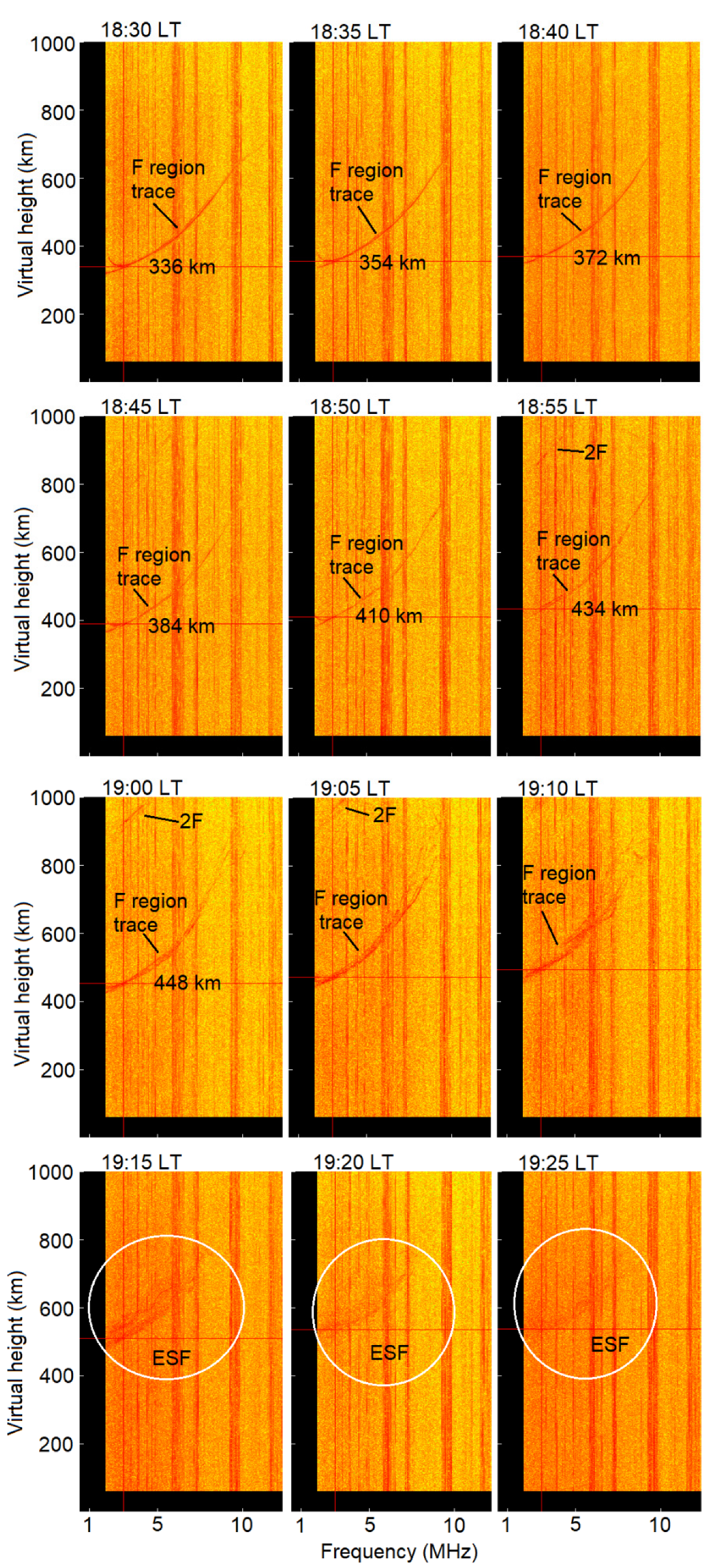
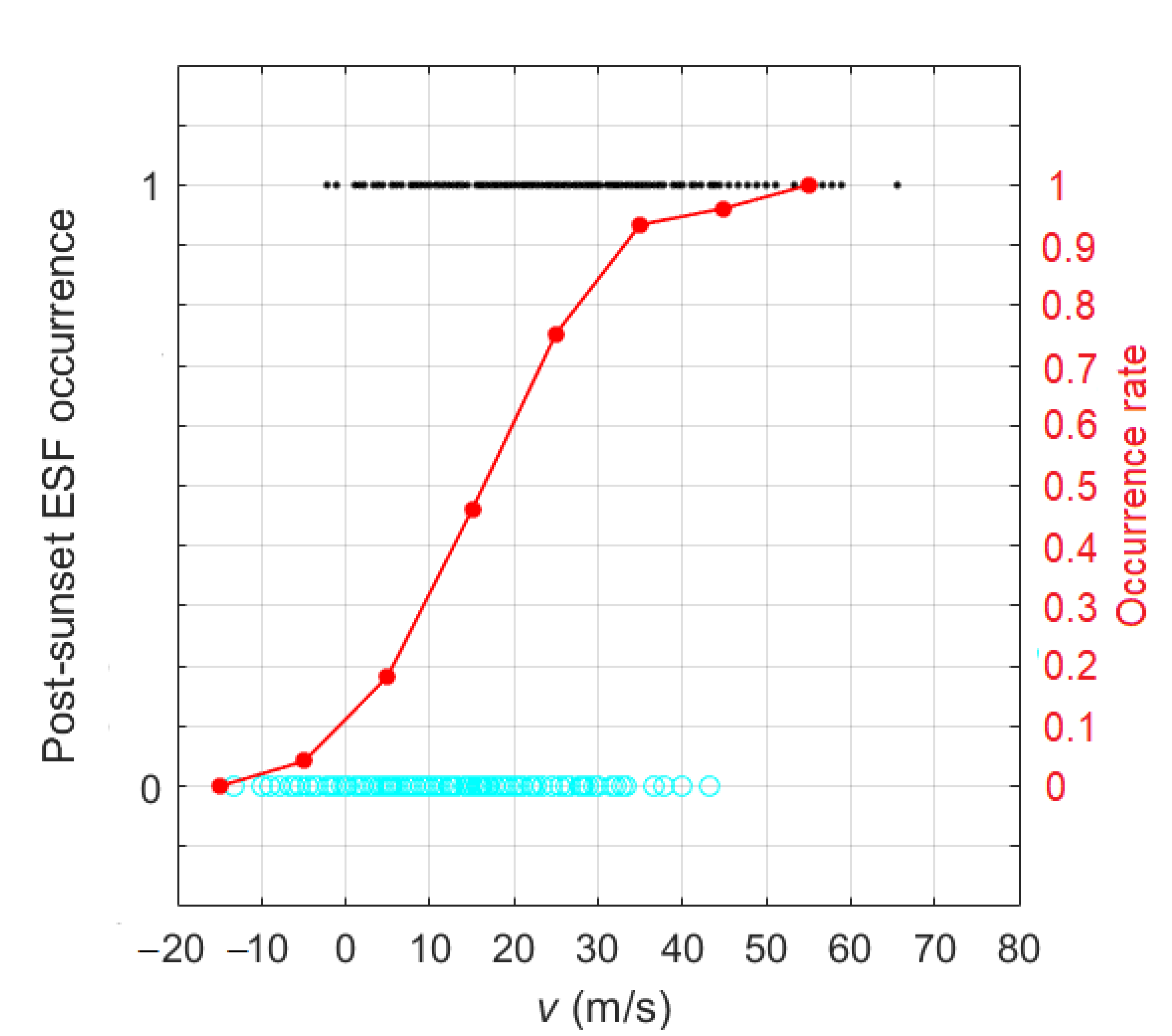
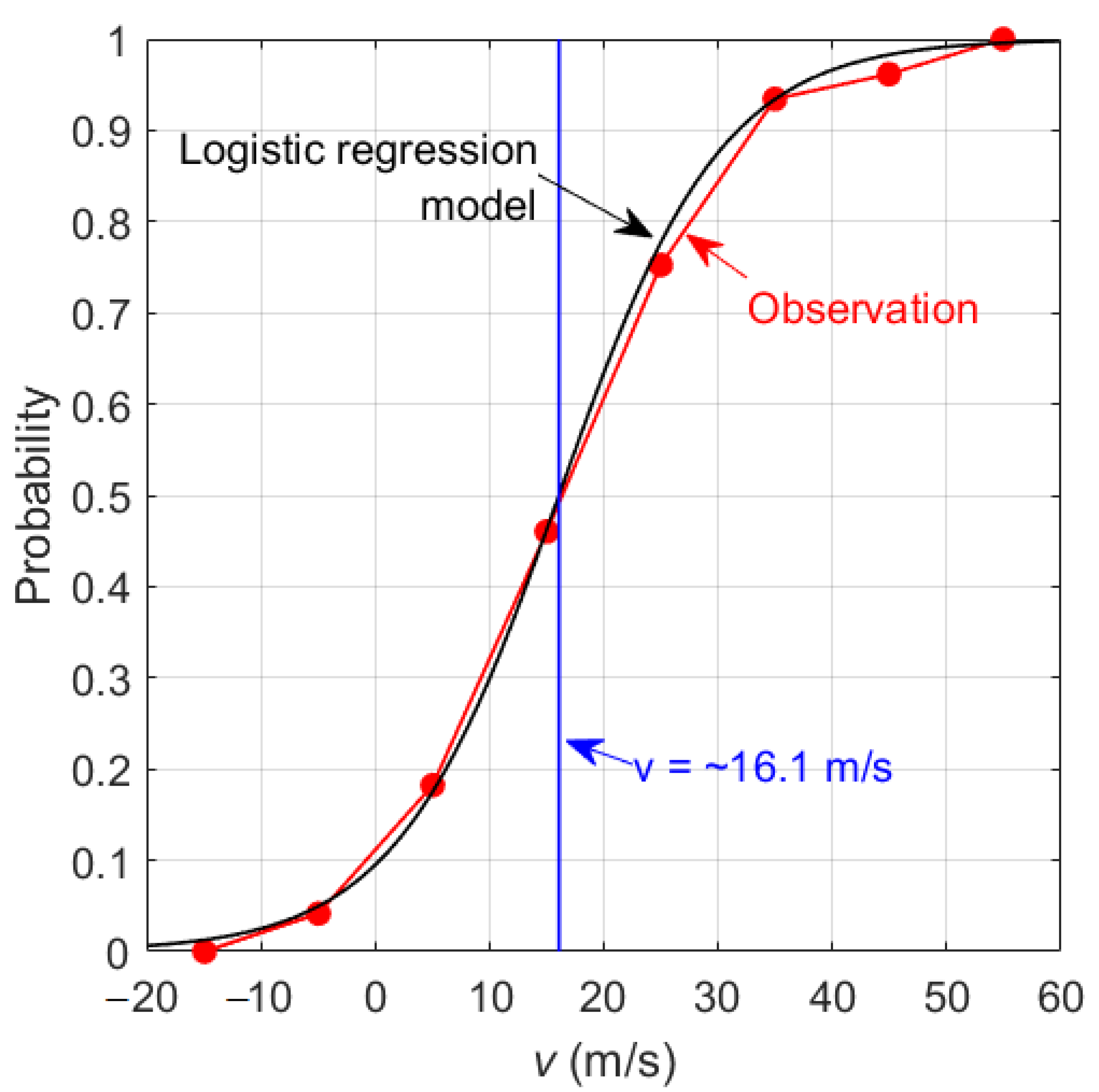
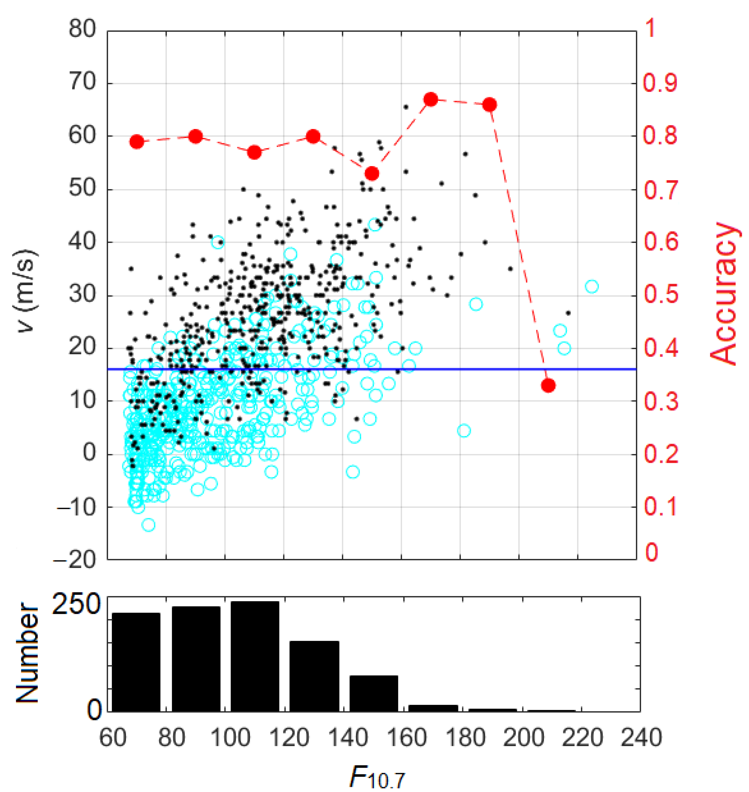
3. Results and Discussion

This study employed the evening upward plasma drift (v) from the ionosondes as a predictor in the model of post-sunset ESF using logistic regression. From these observations, the first results from this study, as displayed in Figure 3, intend to statistically visualize the relationship between v as a predictor and the occurrence rate of the post-sunset ESF. In the panel, the red curve shows the occurrence rate of post-sunset ESFs as a function of v. The occurrence (black dots) and non-occurrence (cyan circles) of post-sunset ESFs were also distinguished by 0 and 1.
Figure 3 shows the occurrence rate of post-sunset ESF at intervals of −20 ≤ v < −10, −10 ≤ v < 0, 0 ≤ v < 10, …, and 50 ≤ v < 60 m/s. The collected 938 data points of v ranged from approximately −13 m/s to 92 m/s, in which v ≥ 60 m/s values indicate the occurrence of post-sunset ESF. The negative v values show the non-occurrence of post-sunset ESF, except for three data points. As for the v values of 0–40 m/s, the occurrence and non-occurrence of post-sunset ESFs overlap. In general, the red curve shows that the probability of post-sunset ESF occurrence increases when v increases. When v increased from a negative value to 30 m/s, the post-sunset ESF occurrence rate increased from 0 to 0.8. The probability of a post-sunset ESF occurrence higher than 0.5 could occur when the v values are greater than 20 m/s. Furthermore, the post-sunset ESF occurrence rates are higher than 0.8 for v ≥ 30 m/s, and these features are consistent with the findings of a previous study [21]. Figure 3 shows a higher correlation between large v and a higher probability of ESF occurrence, and it is a well-known finding. When v is large enough, the necessary seeding mechanisms for generating strong ESF always appear to be present. Therefore, these two phenomena (v and ESF occurrence) are highly correlated [12,13]. However, the relationship between the probability of ESF occurrence and v cannot be simply approximated by linear regression. This study innovates to implement the logistic regression to model the probability of ESF occurrence. Clearly, the red curve in Figure 3 can be approximated by the logistic regression (Equation (1)) and v can be a good predictor of the z-function (Equation (2)).
Next, the result from the training set, that is, the regression coefficients (βj) for the z function (Equation (2)) are shown. Furthermore, the z-function was used in the logistic regression (Equation (1)) to predict the occurrence of post-sunset ESFs. The training set utilized 70% of the dataset, and the remaining 30% was used for the testing set. By steps of the gradient descent technique described earlier, z = −2.25 + 0.14v was obtained from the training set, and this z-function is used in Equation (1) to predict the occurrence of post-sunset ESFs in both training and testing datasets. Figure 4 shows the probability of post-sunset ESF occurrence as a function of v (black curve) calculated from the z-function (z = −2.25 + 0.14v) implemented in logistic regression and the red curve is the occurrence rate of ESF from the ionosondes observation. Note that the red curve in Figure 4 is the same as the red curve in Figure 3. As seen in Figure 4, the black curve closely fits with the red curve. We emphasized that the z-function found is an important finding to model the probability of ESF occurrence. Furthermore, Figure 4 displays the blue line indicating a value of v (~16.1 m/s), and this v can be used to indicate whether post-sunset ESF occurred. With the expression z = −2.25 + 0.14v and logistic regression in Equation (1), the threshold of v (~16.1 m/s) can be found when z is equal to zero. When z ≥ 0, it means that v is greater than/equals ~16.1 m/s and the post-sunset ESF occurrence is expected (the probability ( y ^ ) ≥ 0.5). Otherwise, z is less than zero, meaning that v is lower than ~16.1 m/s, and the post-sunset ESF occurrence is not expected (the probability ( y ^ ) < 0.5). In conclusion, this study suggests that the z-function (z = –2.25 + 0.14v) implemented in logistic regression can be a new technique to predict post-sunset ESF occurrence.
Table 1 summarizes the performances of the z-function (z = −2.25 + 0.14v) or the threshold of v (~16.1 m/s) in predicting the post-sunset ESF occurrence for both training and testing datasets. In addition, Table 1 also shows the performance of predicting post-sunset ESF occurrence using the persistence technique (i.e., what happened yesterday will happen today). The persistence technique is a useful benchmark for model-model comparisons [22]. We have successfully collected 780-data points in our dataset to perform the persistence technique. In the table, the performances are quantified using the accuracy, true positive rate (TPR), false-positive rate (FPR), and true skill score (TSS). Accuracy is calculated from the ratio between the summation of true positives (TP) and true negatives (TN) and the number of data observations. TP is the number of predicted and observed post-sunset ESF events. TN is the number of unpredicted and unobserved post-sunset ESF events. The TPR was calculated as the ratio of TP to the number of observed post-sunset ESF occurrences. Furthermore, FPR = 1 − TNR, where TNR (true negative rate) is the ratio of TN to the number of unobserved post-sunset ESF occurrences. Finally, TSS = TPR − FPR, and the range values of accuracy, TPR, FPR, and TSS are [0 1], [0 1], [0 1], and [−1 1], respectively.
In Table 1, the use of the z-function (z = −2.25 + 0.14v) or the threshold of v (~16.1 m/s) has a good performance in predicting the post-sunset ESF occurrence in the training and testing datasets. As shown in Table 1, the good performance of the z-function can be quantified by higher values of accuracy, TPR, and TSS, along with a lower value of FPR. Interestingly, the performances of the z-function in the training and testing datasets have consistent values. Clearly, the performances of the z-function in both datasets are better than that of the persistence technique. We consider that with an accuracy of ~0.8, TSS of ~0.6, and a better performance than the persistence technique, the z-function used in the logistic regression has a good performance in classifying nights with and without post-sunset ESF occurrence in the training and testing datasets. This finding indicates that the z-function proposed and implemented in the logistic regression (Equation (1)) can be a robust mathematical model to predict the occurrence and non-occurrence of post-sunset ESF on nights when new inputs of v are added. We consider that our mathematical model, like the proposed z-function in this study, can be a prospective tool for nowcasting post-sunset ESF occurrence in space weather services.
In this study, the threshold of v (~16.1 m/s) for determining the occurrence of post-sunset ESF is a statistical finding. It is well-known that the threshold of v for the occurrence of post-sunset ESF could vary with the level of solar activity [23]. Therefore, we need to check the consistency of the threshold of v (~16.1 m/s) in classifying nights with and without post-sunset ESF occurrences with various solar activity levels. Figure 5 shows the scatter plot of v and F10.7 (upper panel) with the occurrence (black dots) and non-occurrence (cyan circles) of post-sunset ESF. Note that 938 datapoints of v and post-sunset ESF occurrence are plotted in the upper panel. The blue line indicates the v of ~16.1 m/s. The figure intends to check the performance of the threshold of v (16.1 m/s) (blue line) in classifying the occurrence and non-occurrence of post-sunset ESF at intervals of 60 ≤ F10.7 < 80 sfu, 80 ≤ F10.7 < 100 sfu, …, and 200 ≤ F10.7 < 220 sfu. Datapoints above or at the blue line will be classified as the occurrence of post-sunset ESF, whereas data points below the line will be classified as non-occurrence of post-sunset ESF. The number of data points (black dots and cyan circles) at each interval of F10.7 is displayed in the lower panel of Figure 5. At each interval of F10.7, black dots and cyan circles highly overlap. However, by calculating the accuracy of the performance of v (~16.1 m/s) in classifying the occurrence and non-occurrence of post-sunset ESF, the red curve in the upper panel shows the accuracy of ~0.8 in F10.7 values ranging from 60 to 140 sfu. The number of data points is 832 in the F10.7 interval of 60–140 sfu. The number of data points for each F10.7 interval above 140 sfu is significantly decreased (below 80 data points), and the accuracy of the performance may not be reliable. In short, the threshold of v (~16.1 m/s) could be reliable for determining whether post-sunset ESF occurred with the accuracy of ~0.8 in the solar activity F10.7 intervals of 60–140 sfu.
The post-sunset ESF occurrence in this study is determined as either the occurrences of RSF or MSF with the spreading trace greater than 30 km in range. The mathematical model of the post-sunset ESF occurrence found in this study could miss predicting the weaker post-sunset ESF occurrences (RSF and MSF with the spreading trace less than 30 km). In addition, the model may have a different accuracy when the threshold of spreading trace in determining the ESF occurrence is changed. The degree of spreading trace in the ESF occurrence can be related to the strength of v, see [24]. We consider that if the threshold of spreading trace is changed to be greater (or less) than 30 km, the threshold of v in determining the post-sunset ESF could be stronger (or weaker) than ~16.1 m/s. As a result, the accuracy of the model changes because the threshold of v in determining the post-sunset ESF occurrence is changed. Furthermore, we would like to discuss the accuracy of 0.8 in our model to predict post-sunset ESF occurrences, and it means that the model could have an error of 0.2 to predict the post-sunset ESF occurrences. As seen in Figure 5, occurrence and non-occurrence of post-sunset ESF highly overlap. Non-occurrence of post-sunset ESF can be occurred either v less than or greater than v of 16.1 m/s. We found that a few points of negative v show the occurrence of post-sunset ESF. On the other hand, we found one data point with stronger v (~40 m/s) showing non-occurrence of post-sunset ESF. The error of 0.2 in our model reflects that the ESF generation could not be controlled by v alone, although v is an important controlling factor for ESF generation. Another controlling factor, such as the presence of large-scale wave structure (LSWS) of plasma density perturbation in the bottom side equatorial F region, could importantly govern the ESF occurrence [25].

4. Summary and Future Works

This study implemented a logistic regression (Equation (1)) with link function z (Equation (2)) containing a linear combination of evening vertical plasma motion (v) to model the post-sunset ESF occurrence. The parameter v is used as a predictor for nowcasting post-sunset ESF occurrence. Data on v and post-sunset ESF occurrences were collected in equinox seasons from the ionosondes in the equatorial zone of Southeast Asia to build the model. From the training dataset, the formalization of z was done as z = −2.25 + 0.14v, and this z function is used in the logistic regression (Equation (1)) to determine whether post-sunset ESF occurred in both the training and testing datasets. From the expression z, the threshold of v (~16.1 m/s) can be derived to expect whether the post-sunset ESF occurred. The values of v ≥ ~16.1 m/s result in positive z, whereas v < ~16.1 m/s results in negative z. When the value of z is greater than or equal to zero (or the y ^ in Equation (1) is greater than or equal to 0.5), the occurrence of a post-sunset ESF is expected. Otherwise, when the z value is less than zero (or the y ^ is less than 0.5), the occurrence of a post-sunset ESF is not expected. With such criteria, the performance of the z function or the threshold of v (~16.1 m/s) found in this study has an accuracy of 0.8 and a TSS of 0.6 for predicting the post-sunset ESF occurrence in both training and testing datasets. The performances of the z-function are better than that of the persistence technique (an accuracy of 0.6 and a TSS of 0.3). This study suggested that the z-function is a statistical finding that can be used to predict the post-sunset ESF occurrence. Here, the z-function found can be implemented in logistic regression for modeling post-sunset ESF occurrence, and this can be a simple and robust mathematical model to predict post-sunset ESF occurrence. The model found in this study can be reliable to predict the post-sunset ESF occurrence in the range of solar flux F10.7 between 60 and 140 sfu.
The mathematical model of the post-sunset ESF occurrence found in this study requires real-time observation of v if it is implemented in space weather services. This work must be complemented by the automatic calculation of v from the ionosonde. Future work needs to develop an automatic scaling of h′ from the ionosonde in the evening sector of the equatorial region. In particular, the automatic scaling of h′ at ~3 MHz for the three ionosondes stations used in this study is required to support the implementation of the model for nowcasting the post-sunset ESF in the space weather services in Southeast Asia. In addition, the mathematical model found in this study should be validated using data observation in solstice months to determine the consistency and accuracy of the model performance.

Author Contributions

Conceptualization, P.A.; methodology, P.A.; software, P.A.; validation, P.A. and Y.O.; formal analysis, P.A.; investigation, P.A., U.A.A. and Y.O.; resources, P.A.; data curation, P.A.; writing—original draft preparation, P.A.; writing—review and editing, P.A., Y.O., U.A.A., P.J., S.P., D.R.M., A.F., R.E.S. and R.R.S.; visualization, P.A.; supervision, Y.O. and U.A.A.; project administration, Y.O. and U.A.A.; funding acquisition, Y.O. and U.A.A. All authors have read and agreed to the published version of the manuscript.

Funding

This research was supported by the 2020 ISEE International Joint Research Program, Nagoya University, Japan. The APC for this manuscript was supported by Telkom University, Indonesia. Y.O. was supported by JSPS KAKENHI Grant Numbers (20H00197; 21H04518). P.J. acknowledges that this research was supported by the Program Management Unit-Brain Power (PMU-B) through the Office of National Higher Education Science Research and Innovation Policy Council (NXPO) under grant no. B05F640197.

Data Availability Statement

Data from the ionosondes of the SEALION project can be accessed at https://aer-nc-web.nict.go.jp/sealion/ (accessed on 15 January 2022). The F10.7 data were obtained from the NASA Omniweb website (https://omniweb.gsfc.nasa.gov/form/dx1.html, accessed on 18 January 2022). The datasets used during the current study, including the MATLAB code for developing the logistic regression model for post-sunset ESF occurrence, are available from the corresponding author upon request.

Acknowledgments

The authors acknowledge the SEALION Project for providing ionosonde observations in the equatorial region of Southeast Asia. The SEALION project was operated with an international effort by King Mongkut’s Institute of Technology Ladkrabang (KMITL), Chiang Mai University (CMU), National Institute of Aeronautics and Space of Indonesia (LAPAN), Institute of Geophysics, Vietnam Academy of Science and Technology (IGP-VAST), University of San Carlos (USC), Kyoto University, Rajamangala University of Technology Isan (RMUTI), and National University of Laos (NUOL).

Conflicts of Interest

The authors declare no conflict of interest.

References

  1. Booker, H.G.; Wells, H.W. Scattering of radio waves by the F region of the ionosphere. J. Geophys. Res. 1938, 43, 249–256. [Google Scholar] [CrossRef]
  2. Kelley, M.C.; Makela, J.J.; Paxton, L.J.; Kamalabadi, F.; Comberiate, J.M.; Kil, H. The first coordinated ground- and space-based optical observations of equatorial plasma bubbles. Geophys. Res. Lett. 2003, 30, 1766. [Google Scholar] [CrossRef]
  3. Xiong, C.; Stolle, C.; Lühr, H. The Swarm satellite loss of GPS signal and its relation to ionospheric plasma irregularities. Space Weather 2016, 14, 563–577. [Google Scholar] [CrossRef]
  4. Aa, E.; Zou, S.; Eastes, R.; Karan, D.K.; Zhang, S.-R.; Erickson, P.J.; Coster, A.J. Coordinated ground-based and space-based observations of equatorial plasma bubbles. J. Geophys. Res. Space Phys. 2020, 125, e2019JA027569. [Google Scholar] [CrossRef]
  5. Cai, X.; Burns, A.G.; Wang, W.; Coster, A.; Qian, L.; Liu, J.; Solomon, S.C.; Eastes, R.W.; Daniell, R.E.; McClintock, W.E. Comparison of GOLD nighttime measurements with total electron content: Preliminary results. J. Geophys. Res. Space Phys. 2020, 125, e2019JA027767. [Google Scholar] [CrossRef]
  6. International Civil Aviation Organization (ICAO). Manual on Space Weather Information in Support of International Air Navigation (Doc 10100); ICAO Publication: Montreal, QC, Canada, 2018; pp. 2-1–2-6.
  7. Alfonsi, L.; Spogli, L.; Pezzopane, M.; Romano, R.; Zuccheretti, E.; De Franceschi, G.; Cabrera, M.A.; Ezquer, R.G. Comparative analysis of spread-F signature and GPS scintillation occurrences at Tucuman, Argentina. J. Geophys. Res. Space Phys. 2013, 118, 4483–4502. [Google Scholar] [CrossRef] [Green Version]
  8. Seo, J.; Walter, T.; Chiou, T.Y.; Enge, P. Characteristics of deep GPS signal fading due to ionospheric scintillation for aviation receiver design. Radio Sci. 2009, 44, RS0A16. [Google Scholar] [CrossRef]
  9. Li, G.; Ning, B.; Otsuka, Y.; Abdu, M.A.; Abadi, P.; Liu, Z.; Spogli, L.; Wan, W. Challenges to Equatorial Plasma Bubble and Ionospheric Scintillation Short-Term Forecasting and Future Aspects in East and Southeast Asia. Surv. Geophys. 2021, 42, 201–238. [Google Scholar] [CrossRef]
  10. Shinagawa, H.; Jin, H.; Miyoshi, Y.; Fujiwara, H.; Yokoyama, T.; Otsuka, Y. Daily and seasonal variations in the linear growth rate of the Rayleigh-Taylor instability in the ionosphere obtained with GAIA. Prog. Earth Planet. Sci. 2018, 5, 16. [Google Scholar] [CrossRef]
  11. Carter, B.A.; Yizengaw, E.; Retterer, J.M.; Francis, M.; Terkildsen, M.; Marshall, R.; Norman, R.; Zhang, K. An analysis of the quiet time day-to-day variability in the formation of postsunset equatorial plasma bubbles in the Southeast Asian region. J. Geophys. Res. Space Phys. 2014, 119, 3206–3223. [Google Scholar] [CrossRef]
  12. Huang, C.S.; Hairston, M.R. The postsunset vertical plasma drift and its effects on the generation of equatorial plasma bubbles observed by the C/NOFS satellite. J. Geophys. Res. Space Phys. 2015, 120, 2263–2275. [Google Scholar] [CrossRef]
  13. Fejer, B.G.; Scherliess, L.; de Paula, E.R. Effects of the vertical plasma drift velocity on the generation and evolution of equatorial spread F. J. Geophys. Res. Space Phys. 1999, 104, 19859–19869. [Google Scholar] [CrossRef] [Green Version]
  14. Dabas, R.S.; Singh, L.; Lakshmi, D.R.; Subramanyam, P.; Chopra, P.; Garg, S.C. Evolution and dynamics of equatorial plasma bubbles: Relationships to ExB drift, postsunset total electron content enhancements, and equatorial electrojet strength. Radio Sci. 2003, 38, 1075. [Google Scholar] [CrossRef]
  15. Abadi, P.; Otsuka, Y.; Liu, H.X.; Hozumi, K.; Martinigrum, D.R.; Jamjareegulgarn, P.; Thanh, L.T.; Otadoy, R. Roles of thermospheric neutral wind and equatorial electrojet in pre-reversal enhancement, deduced from observations in Southeast Asia. Earth Planet. Phys. 2021, 5, 387–396. [Google Scholar] [CrossRef]
  16. Dobson, J.A.; Barnett, A.G. An Introduction to Generalized Linear Model, 4th ed.; CRC Press: Boca Raton, FL, USA, 2018; pp. 149–174. [Google Scholar]
  17. Maruyama, T.; Kawamura, M.; Saito, S.; Nozaki, K.; Kato, H.; Hemmakorn, N.; Boonchuk, T.; Komolmis, T.; Ha Duyen, C. Low latitude ionosphere-thermosphere dynamics studies with ionosonde chain in Southeast Asia. Ann. Geophys. 2007, 25, 1569–1577. [Google Scholar] [CrossRef] [Green Version]
  18. Nozaki, K. FMCW ionosonde for the SEALION project. J. Natl. Inst. Inf. Commun. Technol. 2009, 56, 287–298. [Google Scholar]
  19. Burke, W.J.; Huang, C.Y.; Gentile, L.C.; Bauer, L. Seasonal-longitudinal variability of equatorial plasma bubbles. Ann. Geophys. 2004, 22, 3089–3098. [Google Scholar] [CrossRef] [Green Version]
  20. Piggott, W.R.; Rawer, K. URSI Handbook of Ionogram Interpretation and Reduction; Rep. UAG-23A, World Data Cent. for Sol.Terr. Phys.; NOAA: Boulder, CO, USA, 1972.
  21. Abadi, P.; Otsuka, Y.; Supriadi, S.; Olla, A. Probability of ionospheric plasma bubble occurrence as a function of pre-reversal enhancement deduced from ionosondes in Southeast Asia. AIP Conf. Proc. 2020, 2226, 050001. [Google Scholar] [CrossRef]
  22. Carter, B.A.; Currie, J.L.; Dao, T.; Yizengaw, E.; Retterer, J.; Terkildsen, M.; Groves, K.; Caton, R. On the assessment of daily equatorial plasma bubble occurrence modeling and forecasting. Space Weather 2020, 18, e2020SW002555. [Google Scholar] [CrossRef]
  23. Dabas, R.S.; Lakshmi, D.R.; Reddy, B.M. Day-to-day variability in the occurrence of equatorial and low-latitude scintillations in the Indian zone. Radio Sci. 1998, 33, 89–96. [Google Scholar] [CrossRef]
  24. Abdu, M.A.; de Medeiros, R.T.; Bittencourt, J.A.; Batista, I.S. Vertical ionization drift velocities and range type spread F in the evening equatorial ionosphere. J. Geophys. Res. 1983, 88, 399–402. [Google Scholar] [CrossRef] [Green Version]
  25. Tsunoda, R.T.; Yamamoto, M.; Tsugawa, T.; Hoang, T.L.; Tulasi Ram, S.; Thampi, S.V.; Chau, H.D.; Nagatsuma, T. On seeding, large scale wave structure, equatorial spread F, and scintillations over Vietnam. Geophys. Res. Lett. 2011, 38, L20102. [Google Scholar] [CrossRef]
Figure 1. A sequence of ionograms in the time interval of 18:30 LT–19:25 LT was obtained from the Cebu ionosonde on 31 March 2014.
Remotesensing 14 01896 g001
Figure 2. The distribution of the data collected from Chumphon (CPN), Bac Lieu (BCL), and Cebu (CEB) ionosondes stations during equinox seasons from 2003 to 2016.
Remotesensing 14 01896 g002
Figure 3. The occurrence rate of post-sunset ESF (red curve) as a function of the equatorial evening upward plasma drift (v). The occurrence and non-occurrence of post-sunset ESF are respectively displayed by black dots and cyan circles as well as by 0 and 1.
Remotesensing 14 01896 g003
Figure 4. The probability of post-sunset ESF occurrence (black curve) is derived from the logistic regression and the occurrence rate of post-sunset ESF (red curve) comes from the ionosonde observation. The blue line shows the value of v (~16.1 m/s).
Remotesensing 14 01896 g004
Figure 5. The scatter plot of F10.7 and v (upper panel) with the occurrence (black dots) and non-occurrence (cyan circles) of post-sunset ESF. The blue line indicates v of ~16.1 m/s. The red curve shows the accuracy of the performance of z-function in classifying occurrence and non-occurrence of post-sunset ESF at each F10.7 interval. The number of data points at each F10.7 interval is displayed in the (lower panel).
Remotesensing 14 01896 g005
Table 1. The performances of logistic regression model and persistence technique for forecasting post-sunset ESF occurrence.
DatasetsPerformance
AccuracyTPRFPRTSS
Training
(657 data points)
0.780.790.220.57
Testing
(281 data points)
0.790.790.210.58
Persistence technique
(780 data points)
0.650.680.380.30
Publisher’s Note: MDPI stays neutral with regard to jurisdictional claims in published maps and institutional affiliations.

