
Hyperspectral Indices for Predicting Nitrogen Use Efficiency in Maize Hybrids


1
Corteva Agrisciences™, Indianapolis, IN 46268, USA
2
Lyles School of Civil Engineering, Purdue University, West Lafayette, IN 47907, USA
3
Department of Agronomy, Purdue University, West Lafayette, IN 47907, USA
*
Author to whom correspondence should be addressed.
Remote Sens. 2022, 14(7), 1721; https://doi.org/10.3390/rs14071721
Submission received: 20 February 2022
/
Revised: 21 March 2022
/
Accepted: 29 March 2022
/
Published: 2 April 2022
(This article belongs to the Special Issue UAV Imagery for Precision Agriculture)
Abstract
:Enhancing the nitrogen (N) efficiency of maize hybrids is a common goal of researchers, but involves repeated field and laboratory measurements that are laborious and costly. Hyperspectral remote sensing has recently been investigated for measuring and predicting biomass, N content, and grain yield in maize. We hypothesized that vegetation indices (HSI) obtained mid-season through hyperspectral remote sensing could predict whole-plant biomass per unit of N taken up by plants (i.e., N conversion efficiency: NCE) and grain yield per unit of plant N (i.e., N internal efficiency: NIE). Our objectives were to identify the best mid-season HSI for predicting end-of-season NCE and NIE, rank hybrids by the selected HSI, and evaluate the effect of decreased spatial resolution on the HSI values and hybrid rankings. Analysis of 20 hyperspectral indices from imaging at V16/18 and R1/R2 by manned aircraft and UAVs over three site-years using mixed models showed that two indices, HBSI1 and HBS2, were predictive of NCE, and two indices, HBCI8 and HBCI9, were predictive of NIE for actual data collected from five to nine hybrids at maturity. Statistical differentiation of hybrids in their NCE or NIE performance was possible based on the models with the greatest accuracy obtained for NIE. Lastly, decreasing the spatial resolution changed the HSI values, but an effect on hybrid differentiation was not evident.
1. Introduction
Nitrogen (N) is an essential nutrient for plants and is commonly found in various fertilizer forms to support agricultural production [1]. Unfortunately, the actual N available to maize plants is often much less than the quantity of fertilizer applied, since mineral N availability is affected by a multitude of factors such as precipitation, temperature, microbial effects, soil type, rate of application, placement, timing, fertilizer source, etc. [1]. Even modern hybrids, commercialized after 2000, are only able to recover approximately 50–55% of applied fertilizer, suggesting that much of the applied N is still lost [2]. N recovery efficiencies tend to improve at low N rates but applying lower than agronomic optimum N rates also results in yield declines for growers. Such excessive losses are an economic as well as environmental cost, negatively affecting air and water quality as well as human health [1,3]. Therefore, a large opportunity exists to decrease N use and loss by increasing the efficiency of maize in using this important nutrient.
Although breeding for yield in maize has improved plant N uptake efficiency indirectly [4,5,6,7], greater focused research into plant N efficiency has been encouraged [3]. Crop physiology research has advanced understanding of in-season N dynamics and plant component partitioning and has developed various N uptake and utilization parameters to describe N use efficiency [8,9]. A plant’s N use consists of a multitude of processes such as N uptake, translocation, assimilation, and remobilization. Nitrogen use efficiency (NUE) is a measure of the productivity and agronomic efficiency of plant response to N. For grain producing crops, NUE compares the amount of grain produced by the crop relative to the amount of fertilizer provided to the crop [8,10]. The N parameter of Nitrogen Internal Efficiency (NIE) is one of the two major components of NUE [8,11]. NIE measures the end consequences of season-long N translocation and utilization based on the amount of grain produced by the plant per unit of plant N at maturity. Another important component to a plant’s use of N is the Nitrogen Conversion Efficiency (NCE) parameter, which is a measure of how much biomass a plant produces per unit N in the plant [4,12].
Currently, these N parameters can only be determined via laborious whole-plant field sampling and laboratory-based methods such as Dumas combustion for N tissue determination [13,14,15]. While there have been extensive advances in the field of genotyping during the last 20 years, the current bottleneck to breeding and genetic advancement is in phenotyping [16,17,18]. Efforts to hasten NUE research through high-throughput phenotyping have come to the forefront in recent years due to technological advancements in remote sensing through the use of hand-held or proximal sensing and aerial and ground-based platforms [9,18,19]. Remote sensing is advantageous as it is non-destructive. Additionally, once methods are standardized, it is expected that remote sensing will decrease the labor costs inherent in today’s hands-on phenotyping methods [16,17,20,21].
Hyperspectral sensors commonly collect image data in nearly continuous narrow bandwidths, typically over the spectral range of 300 nm to 2500 nm. Datasets from these sensors contain hundreds of bands, many of which are correlated. The benefit to hyperspectral data is greater spectral resolution, which provides differentiation between materials with absorbance or reflectance characteristics that cannot be discriminated at coarser bandwidths [22].
Image-based vegetation indices (VI) are calculated as reflectance ratios (or ratios of functions of reflectances) at different wavelengths of multi- or hyperspectral data. They are used to predict specific physiological measures [23] or to assess canopy attributes such as leaf area index (LAI) or biomass [24]. Multiple VIs have been well studied in maize for prediction of biomass [25,26,27,28], grain yield [26,27,29,30] and N or chlorophyll levels [15,25,31,32,33,34]. However, direct prediction of the previously described N use efficiency parameters with hyperspectral VIs has not been studied in maize.
The objectives of this study were to: (1) evaluate and identify the statistically best in-season VI(s) for predicting the end-season N use efficiency parameters of NCE and NIE; (2) identify the in-season VI(s) most able to categorize end-season N parameter hybrid differences, as defined by hybrid rankings; and (3) determine the impact of downsampling images from high to low spatial resolution on VIs and the subsequent effect on hybrid rankings.
2. Materials and Methods
2.1. Experimental Design and Site Description
A two-year experiment was conducted during the summers of 2014 and 2017. For 2014 two fields in Woodland, California (CA), (Gorman, 38.751, −121.789; Rominger, 38.727, −121.832) were planted as part of a corn/wheat rotation. Prior to planting and trial establishment, all cover crop and previous crop residue (wheat straw) was removed from the field to further reduce soil organic matter levels and N availability. Soils at Gorman consisted of Yolo silt loam, and those at Rominger field were Brentwood silty clay loam. The 2017 experiment was located at the Agronomy Center for Research and Education (ACRE, 40.483, −86.994) near West Lafayette, Indiana (IN), on land that had previously been planted with soybeans, and consisted of Drummer soils, Milford silty clay loam, and Raub–Brenton complex. Figure S1 shows the general locations of the experimental sites.
The experimental design with a split-plot design (randomized complete block) consisted of 4 replicates and was blocked by N treatment as the main plot. Experiment details are provided in Table 1. N treatments were separated with border plots. Hybrids and plant densities were completely randomized within N treatments. In 2014, nine commercial Mycogen® grain corn hybrids (DAS01 through DAS09), recommended for growing in the Eastern Cornbelt of the United States, were planted in the north–south direction at 2 different densities (65,000 and 95,000 plants per hectare). These hybrids had relative maturity ratings from 99 to 116 days and were selected with an intentionally high amount of genetic diversity. Plots were 6 rows wide (4.6 m) with 76 cm row spacing and 12 m long (not including a 76 cm alley between replicates). Total experiment size at Gorman was 1.8 ha and 1.7 ha at Rominger. At both Woodland, CA locations, all plots were irrigated with drip tape to ensure plants experienced no water stress. Before planting, overhead sprinklers were used to prewet the area. In 2017 five commercial Mycogen® hybrids (DAS02 through DAS05 and DAS09), a subset of those from 2014, were planted at two planting densities, also in the north-south direction (69,100 and 99,600 plants per hectare). The subset of hybrids had relative maturity ratings from 110 to 116 days. Plots were four rows wide (3 m) with 76 cm row spacing and 15 m long, not including a 76 cm alley between replicates. The total experiment size at ACRE was approximately 0.9 ha. The IN experiment was wholly rainfed.
For the 2014 experiment, N fertilizer, urea ammonium nitrate (UAN, 32-0-0), was applied through the irrigation system at a depth of 30 cm. Three N treatment rates were used: 0 kg N ha−1, 56 kg N ha−1 applied at V4, and 224 kg N ha−1. The high N treatment was applied in the following manner: 24.7 kg N ha−1 applied at pre-plant, 50.4 kg N ha−1 applied at V4 and 151.3 kg N ha−1 at V8. In CA, phosphorus (P), potassium (K) and micronutrients were applied at pre-plant using 0-15-15-S-Zn at a rate of 40 kg ha−1 of P or K for the low or medium N treatments. The high N treatment had a pre-plant application of 8-16-8-S-Zn at a rate of 25 kg ha−1 of N or P and 48 kg ha−1 of K. In the IN experiment, N fertilizer (28% UAN) was coulter-band injected between corn rows at physiological growth stage V5. Total N amounts for each N treatment in IN were the same as for the CA plantings. No micronutrients were applied in IN.
The field experiments experienced no visible water stress, and weeds and insects were controlled to avoid additional stress to the plants. Historical and monthly weather data for this experiment are outlined in Table S1. Thirty-year averages were obtained from Woodland (USC00049781), CA, and West Lafayette, IN, stations available from the online data portal of Midwestern Regional Climate Center’s cliMATE system [35]. Monthly averages for ACRE were obtained from the Purdue automated ACRE station, West Lafayette, IN, from the Indiana State Climate Office [36].
Soil testing for N was performed with pre-plant probing of the top 30 cm via two increments of 0–15 cm and 15–30 cm in CA. In IN, soil cores were collected at both V3 and V12 from two depth increments of 0–30 cm and 30–60 cm. CA soil testing was conducted by Dellavalle Laboratory, Inc. (Fresno, CA, USA) using recommended methods for the Western Region [37]. Chemical testing of IN soils was conducted by A&L Great Lakes Laboratories, Inc. (Fort Wayne, IN, USA) using the Mehlich 3 extraction procedure [38] and colorimetry EPA method 350.1 [39] for nitrate determination and the colorimetery EPA method 353.2 [40] for soil ammonia determination.
2.2. Plant Measurements and Physiological N Parameters Measured
Above ground plant sampling and harvest were both carried out on the center 2 rows (rows 3 and 4 in 2014 and rows 2 and 3 in 2017) on the biomass sampling dates in Table 1. In 2014, the center rows were divided into six 1 m long segments (sampling area of 1.22–1.53 m2 of 10–15 plants depending on planting density) for the in-season hand sampling, and one 3 m segment for the R6 sampling zone (sampling area of 4.64 m2 with 30 plants in the low density or 42 plants in the high planting density). All 2014 plots were completely hand harvested. For in-season hand sampling in 2017, the center rows were divided into three 10-plant segments (sampling areas of 1.45 m2 for the low planting density or 1.01 m2 for the high density), each at least 1 m from the others. The 2017 R6 yields were obtained by combine harvesting the center 2 rows after the hand sampling areas had been removed (sampling areas of 18.87 or 20.20 m2). After partitioning plants into leaves, stalk/tassel, and ears (if present), plant parts were dried at 65 °C to constant weight. Then, moisture and weights were determined and samples ground to 1 mm. N concentration (pN) (%) of samples (stover or grain) was determined through Dumas combustion at the Dow AgroSciences Analytical Laboratory for the 2014 samples (Indianapolis, IN, USA) and A&L Great Lakes Laboratories, Inc. for the 2017 experiment. All grain yield is reported at 15.5% moisture.
The N parameters were calculated based on the following relationships using field sampling and laboratory N analysis data obtained as described above.
Nitrogen Conversion Efficiency (NCE) (kg kg−1N):
where BMtot = whole-plant above ground biomass weight and Nplant = total plant N content.
NCE = BMtot/Nplant,
Nitrogen Internal Efficiency (NIE) (kg kg−1N):
where Y = grain yield at 0% moisture and Nplant = total plant N content.
NIE = Y/Nplant,
2.3. Remote Sensing Data
All remote sensing data acquired over the 2014 fields in CA were collected by SpecTIR LLC, based in Reno, Nevada, from a manned aircraft flown at 405 m at Gorman and 410 m at Rominger on the dates shown in Table 1. The hyperspectral camera was a ProSpecTir-VS pushbroom system with a spectral range of 390 to 2450 nm at 5 nm (360 bands) and a 320-pixel swath. Swath width was approximately 160 m, and spatial resolution was 0.5 m for this data set. All data were collected with the sun at ≥40° elevation angle. Data for this study were acquired in a single flightline. ATCOR® (Atmospheric and Topographic Correction) software was used to convert the radiance data to reflectance values, and spectral polishing was achieved using a proprietary program based on the Savitsky–Golay filter. Geocorrection was based on a 12-channel GPS system with real-time differential corrections provided to the inertial navigation system (INS). A 10 m resolution digital elevation model was used to orthorectify the images. Data were provided in the UTM Zone 10–WGS–84 map projection and datum.
At ACRE, hyperspectral data were acquired at desired physiologically relevant times (Table 1) by a Nano-Hyperspec® VNIR pushbroom scanner (Headwall Photonics, Inc., Bolton, MA, USA) mounted on a DJI Spreading Wings S1000 octocopter (DJI, Nanshan District, Shenzhen, China). The octocopter was flown approximately 60 m above the ground at 8 m s−1 velocity, resulting in a 24 m field-of-view (640 pixels per scan line). Each image had 272 bands (400 to 1000 nm spectral range), 4 cm spatial resolution and 2.2 nm spectral resolution. An Applanix APX-15 V3 GNSS/INS unit (Applanix, Richmond Hill, Ontario, Canada) provided navigation information. Hyperspectral data were orthorectified based on a 1.0 m digital elevation model (2011–2013 IN statewide LiDAR, IndianaMap Framework Data) using the Headwall Photonics SpectralView software and processed to reflectance using FLAASH in the ENVI software (L3Harris Geospatial Solutions, Inc., Broomfield, CO, USA). Individual flightlines were mosaicked with ENVI 5.5 software. As an initial investigation, data from images at similar phenotypic time points across all 3 locations were grouped. Specifically, imaging data from V18 in CA were grouped with imaging data from V16/17 in IN. Similarly, R1/R2 data from CA were pooled with imaging data from IN at R1.
2.4. Feature Extraction with Hyperspectral Indices (HSI)
As the 2014 CA images had lower spatial resolution (50 cm), the 2017 IN images were downsampled spatially by averaging the spectral values of all the pixels in each 50 × 50 cm spatial area. This enabled comparison of images and data of similar spatial resolution for similar phenotypic time points. Indices shown in Table 3 were calculated. The 20 hyperspectral vegetation indices (HSI) were chosen based on literature references documenting respective investigations for predicting plant biomass, chlorophyll or N concentration, grain yield, or plant stress. These HSI were based on spectral regions known to be responsive to plant performance changes. Imaging data were binned to ~5 nm for all HSI calculations to reduce noise. However, bands at 855 and 910 nm for HBSI1 and HBSI2, respectively, were binned to 20 nm as recommended [27]. Soil pixels were removed using thresholds developed for each imaging date and location. The threshold value selected to identify soil pixels was based on inspection of the image, known soil locations, and the reflectance histogram of each index. For each plot of maize in the imaging data, subplots of the inner 2 rows were extracted, avoiding the areas within 1 m of the alleys and in-season sampling areas. This resulted in subplots 152 cm wide and approximately 6.5 m long. Finally, the remaining pixels within these subplots were averaged to obtain the final HSI reflectance data for each plot. The high spatial resolution imaging data from IN were processed similarly for generation of the HSI.
2.5. Statistical Analysis
Statistical analysis was based on JMP 14.3.0 and SAS Enterprise Guide 7.1 (SAS Institute Inc., Cary, NC, USA). Mixed models (PROC MIXED) with the Restricted Maximum Likelihood Method (REML) were used in the analysis. Model assumptions of constant variance and normality were evaluated visually [56]. When necessary, values were transformed to satisfy model assumptions and parametric bootstrap procedures were used to estimate confidence limits (1000 bootstrap samples).
2.5.1. Treatment Effects
Mixed models were developed to examine the effects of the N treatment, plant density, hybrids and their two-way interactions on the physiological parameters of total biomass at R6 (TDM), N concentration at R6 (pN), total nitrogen content (TNC), or grain yield at R6 (GY), with a significance level of α = 0.10. Each model had hybrid, N treatment, plant density, and their 2-way interactions as fixed effects. Random effects included environmental effects, including location, block(location), location * hybrid, location * plant density, and location * N treatment. Random effects were removed when they accounted for less than 1% of the total variance within the data. Analyses for the physiological parameters (TDM at R6, pN at R6, TNC at V12, R1 and R6, and final GY) were conducted for the data “globally” across all three site-years, accounting for location effects through the random effects in the mixed model. Sample means were compared for statistically significant fixed effects in the mixed models based on a Tukey–Kramer HSD means comparison at α = 0.10.
2.5.2. Hybrid Rankings
Comparison of the hybrid’s relative response in the N parameters (Y = pN, TNC, NCE or NIE) to the environment and treatment effects was established through mixed models with hybrid, N treatment, plant density, and 2-way interactions as fixed effects. Hybrid rankings were ascertained by globally grouping all three locations, as well as for the ACRE location-only, to allow for comparison in the spatial resolution analysis described in the following sub-sections. For the global analysis of all locations, environment was the random effect (block(location), location, location * hybrid, location * N treatment). For the ACRE-only analysis, environment random effects were pass and block only. The term “pass” refers to the row location of each treatment on a plot map. Rankings for the N parameters were defined when the fixed effect of hybrid was significant at α = 0.10 in the model, and there was hybrid separation based on a Tukey–Kramer HSD means comparison (α = 0.10).
2.6. Relationship of HSI to N Parameters
2.6.1. HSI Selection
Relationships between the 20 in-season HSI and each of the end-season N parameters were explored by location based on the Pearson correlation coefficients (r) and the Spearman (non-linear) rank correlation coefficients (r). Sign and magnitude of correlation coefficients for each of the three locations were evaluated. HSI were selected for further statistical analysis when all three locations were positively or negatively correlated and at least one location had a Pearson correlation coefficient approximately ≥ |0.30| (magnitude) (step A in Figure 1).
Mixed models for predicting the N parameters (dependent variable, Y) across all three site-years consisted of the HSI at a defined time point (V16/18 or R1/R2) along with hybrid and hybrid * HSI as the fixed effects. Random effects included location only to avoid overfitting the model. Treatment effects such as plant density and N fertilizer were not included due to confounding effects in the statistics models.
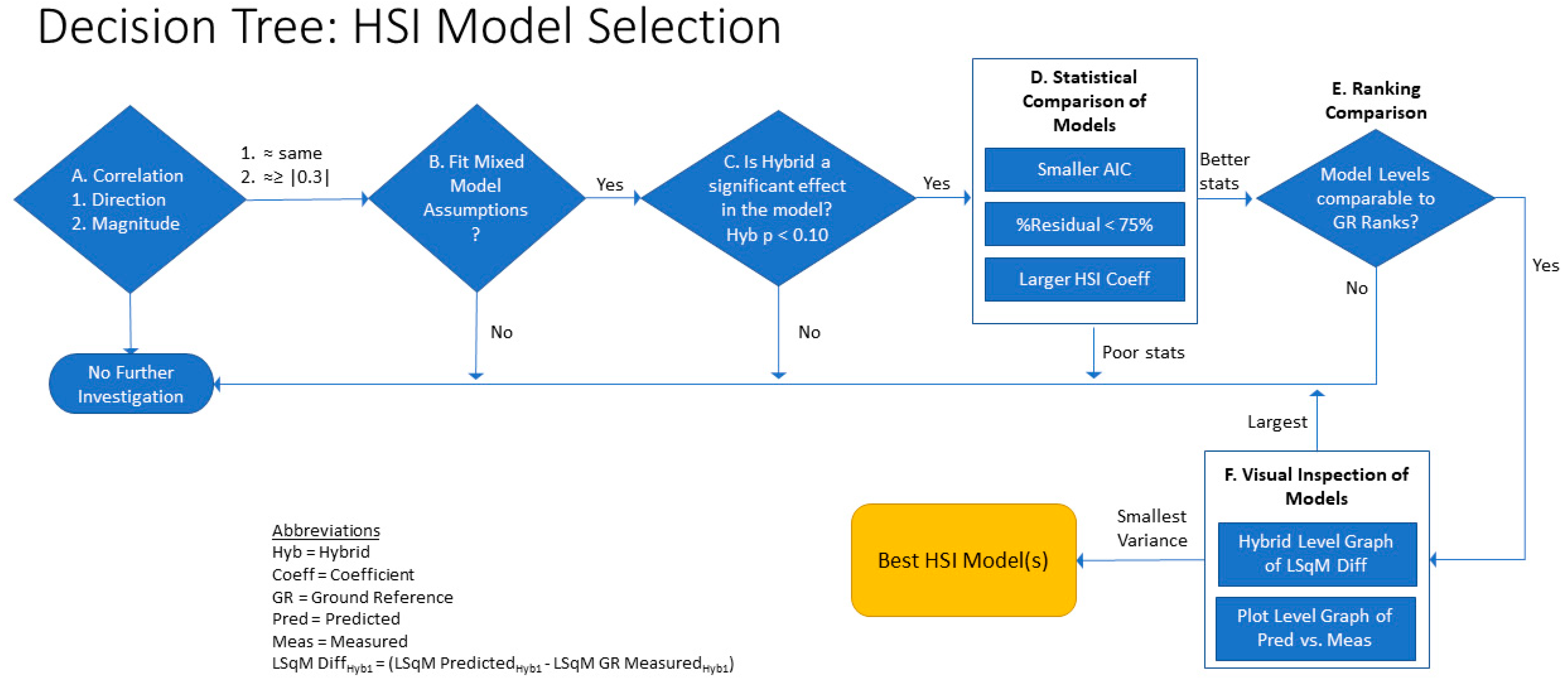
Values of indices were standardized to mean = 0, std dev = 1 to facilitate comparison, defined as z-scores. A decision tree based on six criteria described below (see Figure 1) was used to select the best HSIs for predicting the N parameters:
- A.
- Survey correlation statistics based on sign and magnitude as described in Methods;
- B.
- Examine residual diagnostics, selecting HSI models where statistical assumptions are satisfied;
- C.
- Select models where hybrid is a significant effect at α = 0.10;
- D.
- Compare statistical values of each model with preference for models with smaller Akaike’s Information Criterion (AIC), % residual <75%, and larger coefficient estimate for the standardized (z-score) HSI effect;
- E.
- Compare hybrid ranking level letters (obtained from a Tukey–Kramer’s HSD means comparison) of the HSI model to the ground reference hybrid rankings;
- F.
- Visually inspect charts of the difference in the hybrid least square mean values of the HSI and ground reference models as well as plots of the predicted by measured values at the per-plot level; preference is given to the models with smallest variance.
2.6.2. Impact of Downsampling
The impact of reducing spatial resolution of the ACRE hyperspectral data was evaluated using a matched pairs t-test (α = 0.05) in JMP based on those indices identified as most predictive of the N parameters from the previous section. Downsampling effects on hybrid rankings were established by evaluation of Pearson correlation coefficients as well as building mixed models similar to those used for predicting the N parameters from the HSI in the global analysis described previously (Y = N parameter; fixed effects: HSI, hybrid, and hybrid * HSI; random effects: pass and block). Models were developed using both the high and low resolution standardized HSI data. Rankings were based on the hybrid least square means estimates and Tukey–Kramer means comparison (α = 0.10) obtained from the mixed models. The ground reference hybrid rankings and those obtained for the high- and low-resolution models were compared.
3. Results and Discussion
3.1. Treatment Effect on Physiological Parameters
Models for analyzing the treatment effects on the agronomically important physiological parameters of biomass (TDM), total N content (TNC) and yield are shown in Table S3. Least square mean estimates of TDM and TNC (at V12, R1 and R6) by the main fixed effects (hybrid, N, plant density) are reported in Table S4. Since these variables were not central to the key theme of our study, results are discussed in the Supplementary Materials.
As a measure of the final impact of the (main fixed) treatment effects, the mean estimates of grain yield are shown in Table 4 along with the Tukey–Kramer HSD means comparisons. Hybrids for these experiments were specifically selected to be genetically diverse, and DAS03 and DAS08 had significantly higher grain yield estimates than DAS09 and DAS07. Hybrid differences in response to N are well documented [57,58]. Although grain yields (averaged across hybrids, plant densities, and 3 site-years) increased numerically with higher N rates as anticipated, the response to N fertilizer was not statistically significant.
3.2. Treatment and Time Effect on N Parameters
3.2.1. Effect on pN at R6: Ground Reference Model
The model built on the agronomic data for prediction of whole-plant N concentration at R6 (pN) explained more than 80% of variability in the data (Table 5). Location accounted for the largest proportion (~60%) of the variability in the data and the interaction between N and location accounted for more than 20%. All fixed effects (main effects and interactions) were significant in the model except for the interaction between N and plant density. Significant hybrid differences were evident upon Tukey–Kramer analysis resulting in three levels (A, B, and C) (Table 4). Similar whole-plant pN hybrid differences have been observed in previous research on N and genotypes [4,59]. In our study DAS06 had significantly higher pN than DAS03, DAS04, and DAS07. However, several hybrids (DAS01, DAS02, DAS05, and DAS08) were indistinguishable from the highest and lowest ranked hybrids. The statistical separation of hybrids based on pN motivated the analysis of HSIs for predicting this N parameter in our study.
3.2.2. Effect on NCE: Ground Reference Model
Over the three site-years, the mean NCE increased over the growing season from 51.3 kg kgN−1 at V12 to 107.3 kg kgN−1 at R6. This was similar to previous studies documenting maize biomass increases, even under N stress [60]. An increase in standard deviation of NCE at R1 was driven by an increase in the standard deviation for both plant dry matter (PDM) and TNC, the two NCE components. Over the growing season, the variance of the distribution of NCE increased and became skewed to higher values by the season’s end (R6). This was driven by an increase in the standard deviation in TNC from R1 to R6, which also skewed to higher values. The increase in TNC from R1 to R6 shows differences in post-silking N uptake for the different hybrids. Lower NCE values under high N conditions throughout the growing season are consistent with prior research, which shows NCE increasing more for low N than high N over the season [4,61]. The range in NCE between hybrids (12.3 kg kgN−1) or N treatments (26.0 kg kgN−1) was similar to research evaluating hybrids released over a 38 year span at similar N fertilizer rates [4]. In contrast to that study, however, our experiment had a 0N treatment; thus, an increased range of N treatment response was expected. The relatively small grain yield response suggests that our sites may have had considerable available N even at the 0N rate. Stronger results may have been obtained with prior N drawdown management of the 0N fields.
3.2.3. Effect on NIE: Ground Reference Model
The overall NIE mean (at R6) of all three site-years across all N treatments was 50.2 kg kgN−1. At low N rates, the NIE distribution was skewed towards higher values with a high mean NIE (55.0 kg kgN−1). The medium N treatment NIE mean was 51.0 kg kgN−1. The high N treatment had a more symmetric distribution and a lower mean NIE (45.8 kg kgN−1). This decreasing NIE response with an increase in N treatment is well documented in other research [11,62]. The difference in NIE between the low and high N treatment in our experiment (9.1 kg kgN−1) was similar to some N research in maize [4,11] yet much smaller than other research [62]. Since these studies had comparable fertilizer treatments this indicates a wide range of N treatment (low N, ~0 N to high N, ≥220 N) is important to differentiation, but not the only factor necessitating consideration in designing the experiment for delineation between hybrids.
The range in NIE response (9.9 kg kgN−1) between hybrids in our study was similar to other research evaluating hybrids commercialized from 1967 to 2005 [4] but much lower than the response evident in a longer era study (69 yrs) of maize hybrids [2]. This suggests our research may have had stronger results with greater genetic differentiation in our hybrids.
3.2.4. Hybrid Rankings by NCE or NIE at R6
Agronomic models for predicting ground reference NCE or NIE accounted for ≥80% of the variability in the data (Table 5). These models indicated that location alone accounted for the majority of the variability in the data. The main effects of hybrid and N were significant to both models while plant density was only a significant effect for NCE. Thus, hybrid and N treatment had significant impacts on NCE and NIE. These results of hybrid effect on NCE or NIE agree with previous results showing the genotype impact [4,63].
Significant differences in NCE between hybrids were evident based on Tukey–Kramer means differences for both the global or ACRE-only data (Table 6). Hybrids DAS04 and DAS07 had the highest NCE values. They were significantly larger than DAS06 and DAS09, the two lowest ranking hybrids by NCE. The ACRE model provided slightly different hybrid rankings. As in the global model, DAS03 ranked significantly better than DAS09. However, while DAS04 was one of the highest ranked hybrids in the global model, at ACRE it was not significantly different from the poorly ranked DAS09. Numerically, DAS04 had higher NCE than DAS09 at ACRE. This difference between the models highlights the importance of testing hybrids across multiple environments to provide a broader perspective of a hybrid in a grower’s field and to have greater statistical confidence of a hybrid’s performance.
Significant differences in NIE between hybrids were also evident though with fewer difference levels: three across the nine hybrids (Table 6). DAS03 was highest in NIE. The lowest tiered hybrids, significantly different from the top tier, were DAS05 and DAS07. DAS03 also had significantly higher NIE than DAS06 and DAS09. At ACRE-only, DAS03 was also significantly higher in NIE than DAS09. However, the distinction between DAS03 and DAS02 at ACRE was not apparent in the global model.
3.3. Evaluating the Relationship between N Parameters and Hyperspectral Indices
Exploratory investigations into the relationship between the N parameters (pN, NCE and NIE) and the HSI noted that for many HSI there were differences in the distribution of the spectral indices obtained each year. Based on the experimental design, potential causes for such distribution differences could be imaging platforms, weather (in 2014 vs. 2017) or agricultural locality (California valley basin vs. Eastern Cornbelt). Due to previous results of the importance of location, all data were evaluated for correlations by location.
3.4. Correlation between N Parameter (pN, NCE, NIE) and HSI
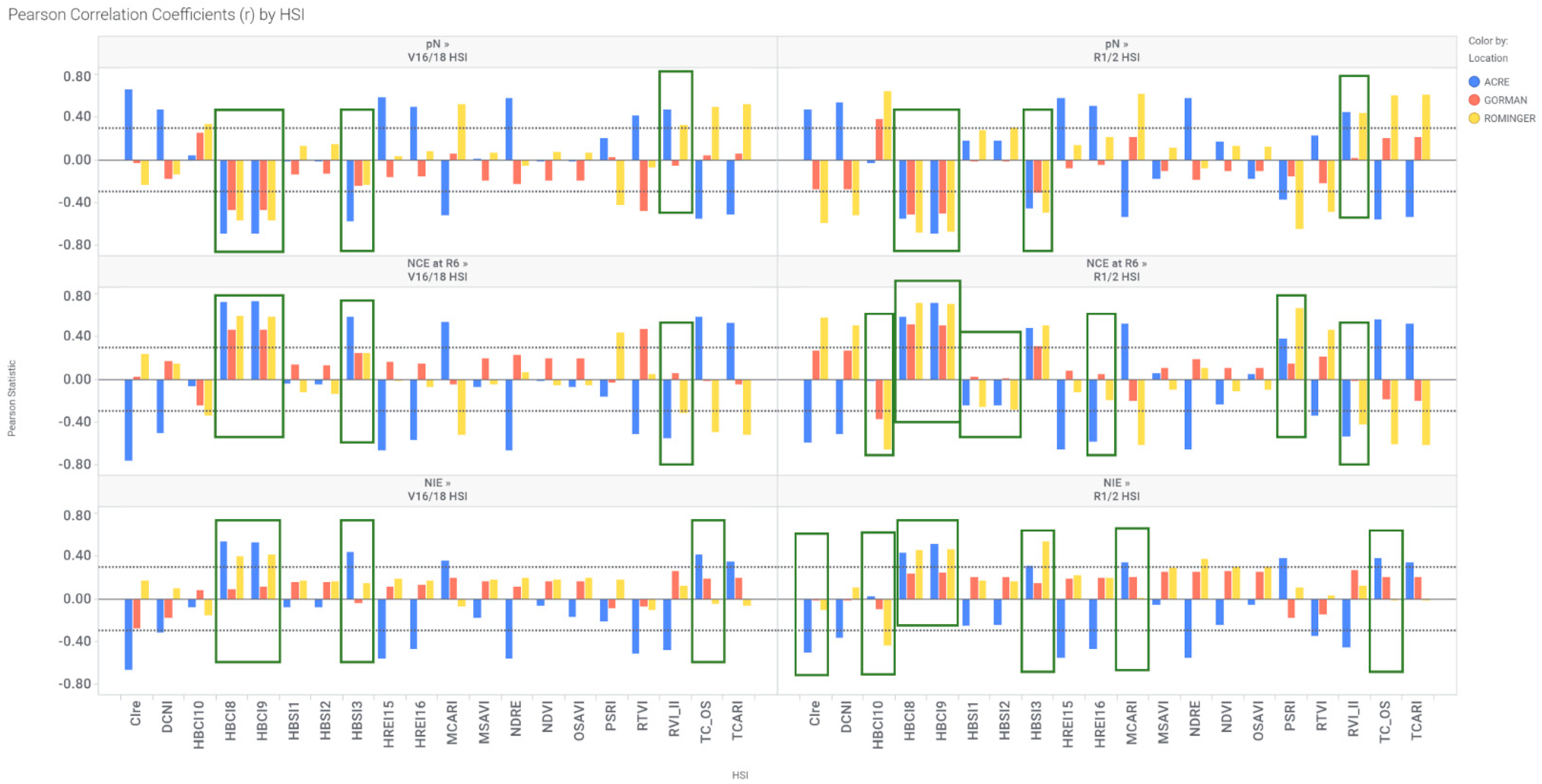
Pearson correlation coefficients between the three N parameters at R6 and the HSI at V16/18 and R1/2 for each location were evaluated (Figure 2). Initial observations showed very few of the 20 HSIs were strongly correlated (r > 0.6) with the N parameters at all three locations. Similarity in sign and magnitude of correlation were more evident between Gorman and Rominger, the two CA locations, than with the IN location. However, several HSI (15 for pN, 16 for NCE, and 14 for NIE) were selected for further investigation based on the criteria of consistent directionality (sign) and magnitude of correlation (step A in Figure 1). Spearman’s rank correlations (data not shown) and the Pearson correlation coefficients had the same signs. As hypothesized, the HSI that were more strongly correlated to pN were also those most strongly correlated to NCE and NIE. Since N deficiency can cause plant stress, it was surprising that none of the plant stress HSIs (HREI15, HREI16, NDRE, and CIRE), were highly correlated with pN at any of the three locations. This result was in contrast to previous studies which showed CIRE and other red edge HSIs reliably predicting N content in plants with low N levels [34,64]. DCNI, an HSI developed for N detection by [48], was also not strongly linearly related to pN. However, our findings supported work by [65] who found poor predictability for plant N with this index. Previous findings of chlorophyll indices such as MCARI, TCARI, and TCARI/OSAVI that were strongly correlated to leaf chlorophyll at the canopy scale [66,67] were not supported by our results, which found that these HSI had inconsistent or small correlations with pN.
Correlation coefficients were often larger for pN and NCE, relative to NIE, especially at ACRE. Since NCE is the amount of dry matter per unit of N in the plant, an analysis of variance was conducted to evaluate whether there was less dry matter in 2014 than in 2017 to account for the stronger correlations observed in 2017. This would suggest that the HSI are simply sensing biomass differences in the fields. Welch’s Anova for the model with year as the independent variable indicated significant differences (α = 0.05) between years at V12 and R6 for plant dry matter (PDM) and at R6 for TDM. However, at both plant stages the biomass in 2014 was greater than in 2017. This pattern was opposite to that from the HSI correlation suggesting the indices were not just sensing biomass differences between years. An analysis of the statistical difference in plant N (TNC) by year indicated that at all time points (V12, R1/R2, and R6) TNC in 2014 was statistically greater than in 2017 suggesting N detection was driving the stronger NCE correlations with the indices (Welch’s Anova and ANOVA, α = 0.05). There were no obvious changes in the magnitude of the correlations between HSIs and NCE at V16 or R1. Conversely, for NIE the correlations changed depending on the HSI and imaging time point, suggesting some indices may be more sensitive to NIE changes and thus better predictors.
3.5. N Parameter Estimation by HSI
3.5.1. Predicting pN with Hyperspectral Indices
Of the 15 plant-stage HSI models selected based on the value of the correlation coefficient between pN at R6 and HSI, only five fit the mixed model statistical assumptions (normality and constant variance) (step B in Figure 1): HBCI8 at V16, and HBCI8, HBCI9, HBSI2, and HRE16 at R1. However, for two of the five models, hybrid was not a significant effect; thus, these models (HBCI8 and HBCI9 at R1) were not considered further (step C). The AIC value (−134.2) for V16 HBCI8 was low but the residual was large (98.1%) so this model was not investigated further (step D). The statistics for the remaining two models (HBSI2 and HREI16 at R1; Table 7) were similar; thus, the next consideration was the hybrid rankings (step E).
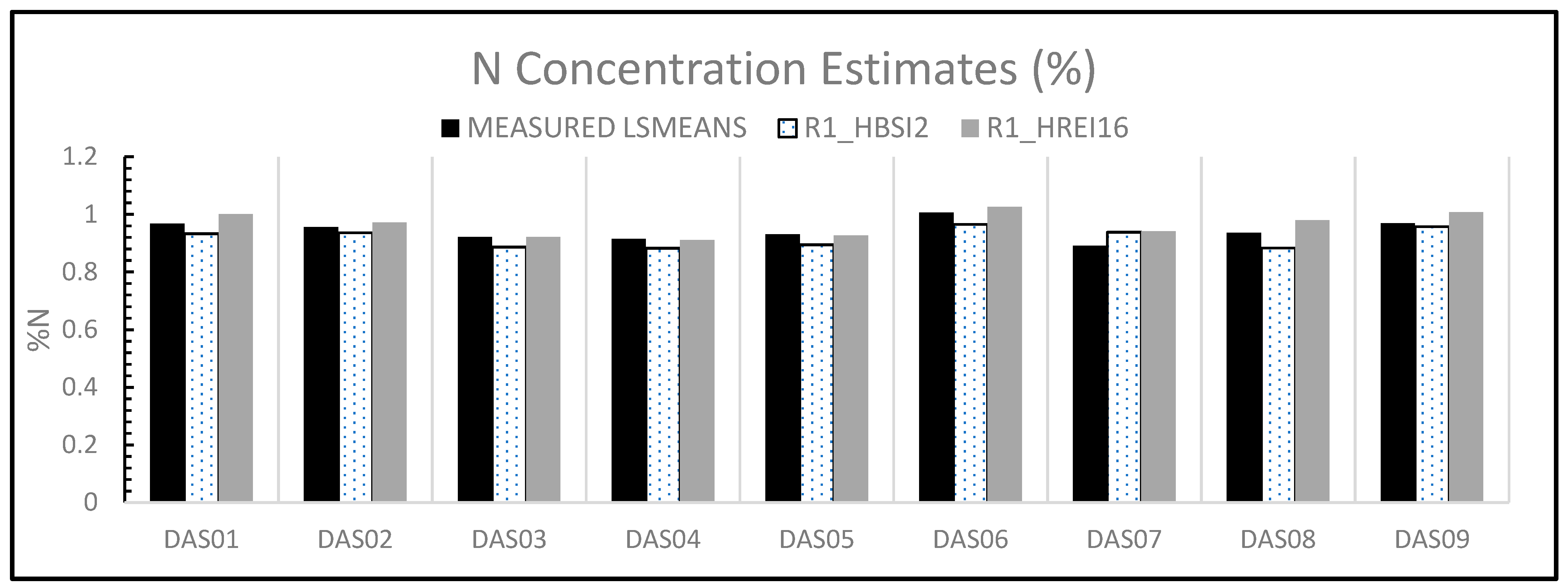
The hybrid rankings based on ground reference pN resulted in three levels (A, B, and C) shown in Table 7. The two HSIs identified as predictive of pN, HBSI2 and HREI16 at R1 both resulted in two levels. HBSI2 only clearly differentiated between DAS09 and DAS04. This model was unable to discriminate between DAS06 and DAS07. Similarly, while HREI16 distinguished between DAS06, DAS03, and DAS04 as in the reference model, it also, did not differentiate between DAS06 and DAS07. Thus, the hybrid rankings for pN by either HSI were not consistent with the reference data.
Visual inspection of the plots (step F) illustrated the statistical results. Figure 3 shows that R1 HBSI2 underestimated the hybrid means, while HREI16 consistently overestimated them. Overall, R1 HBSI2 had the smallest predicted difference in the means for all hybrids except for DAS07. Interestingly, DAS07 was the hybrid with the least accurately estimated pN by both models. The cause of the poor estimates for DAS07 is unknown. Inspection of the parentage of these hybrids reveals that DAS07 was the only hybrid with a different female inbred, hinting at the potential interaction of genotype and HSI. More evidence of this interaction is needed.
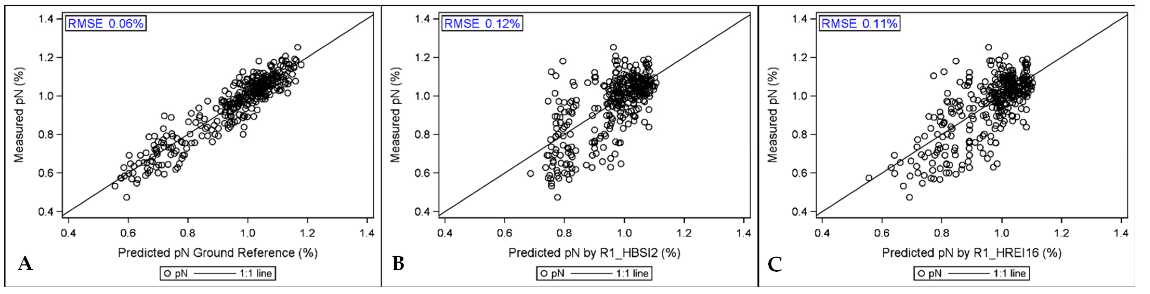
The predicted vs. measured graph based on each of the selected HSI is shown in Figure 4. The individual by-plot estimates have slightly lower variance of the residuals for HREI16 than HBSI2, especially at the lower pN. The least square hybrid means shown in Figure 3 indicate HREI16 was the most accurate HSI model for pN at the hybrid level. Figure 3 and Figure 4 show the models are similar in predictions, but the indices have too much noise for practical implementation. Additionally, the HBSI2 range is not small enough for accurate predictions. Based on these comparisons, HBSI2 and HREI16 at R1 were the best HSIs for predicting pN within those evaluated. However, neither was able to clearly separate hybrids at R6 based on in-season imaging.
3.5.2. Predicting NCE with Hyperspectral Indices
Based on correlation values, 15 HSI-time point combinations were evaluated for predicting ground reference NCE values. The analysis delineated in the decision tree of Figure 1 was followed as described in detail for pN. Only four HSI, HBSI1, HBSI2, HBSI3 and HBCI9 at R1, had adequate fit to the model assumptions. Constant variance was usually the assumption violated by the other models, removing them from consideration. Further analysis indicated HBSI1 and HBSI2 had the best performance. The hybrid rankings and fit statistics are shown in Table 8. The reference data hybrid rankings clearly show DAS07 = DAS04 > DAS09 = DAS06 (Table 8). The models for HBSI1 and HBSI2 only showed two levels in the rankings. However, both models identified DAS04 > DAS09 = DAS06. Consequently, some of the differentiation from the HSI models matched the reference rankings even though separation of DAS07 was missed by the HSI models. All other hybrids were inseparable based on both HSI models.
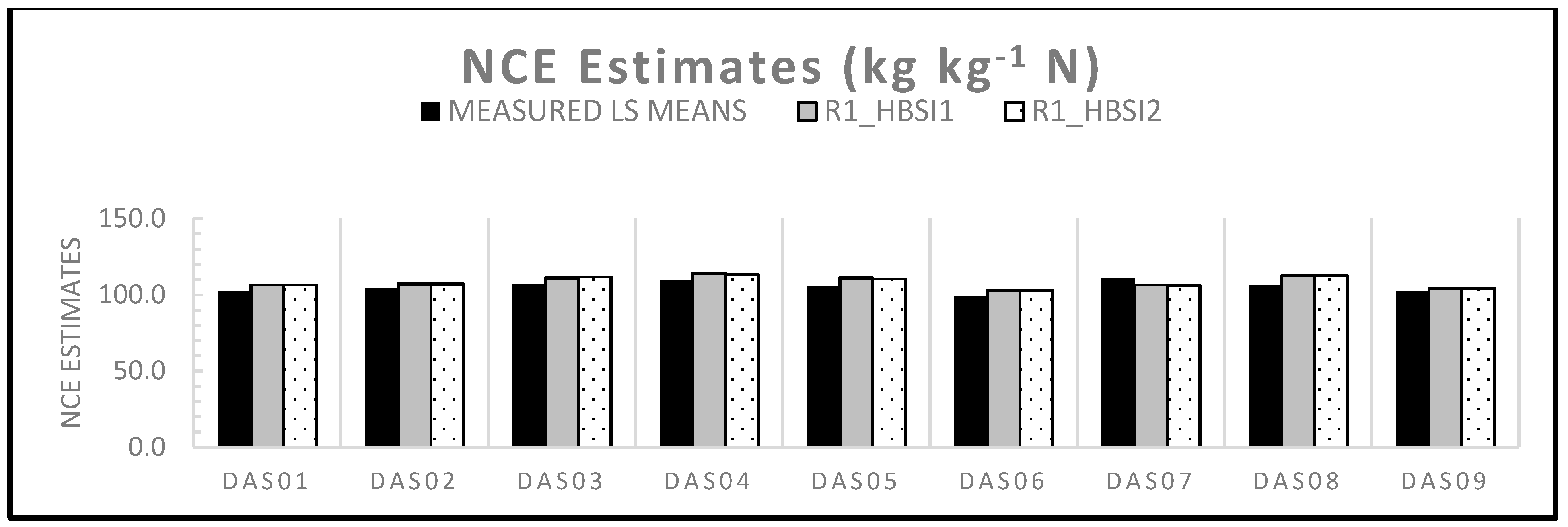
Plots of the hybrid LS means show comparable estimates between HSBI1 and HBSI2 (Figure 5). Most of the predictions for HBSI1 and HBSI2 were greater than the measured means. DAS07 was again an outlier, consistently underestimated by both models. By plot, the scatter pattern was similar for both HSI with greater scatter in the larger measured NCE values (>125 kg kgN−1) (Figure 6). However, the overall by-hybrid estimates in Figure 5 based on the in-season HSI imaging were quite similar to the measured end-season ground reference means. Removal of the lowest ranking hybrids (DAS06 and DAS09) by either HSI model resulted in a hybrid pool still containing the top five hybrids by NCE. In summary, both of these HSIs succeeded in providing ranking guidance for culling two of the lower performing hybrids (DAS06 and DAS09) for end-season NCE based on R1 imaging data.
Both HBSI1 and HBSI2 are normalized difference vegetation indices with NIR reflectance at 855 or 910 nm, respectively. The NIR region is known for detecting variations in cellular structures and plant cavities which vary upon changes in plant vigor or health. These experiments were designed to cause N stress to the maize plants over time. This effect is evident in the low N treatment of our experiment which had significantly lower biomass (TDM at R6), pN, and TNC at R6 as well as numerically lower grain yields. NCE is closely tied to plant health since it is a measure of biomass produced per unit of N. Consequently, this newly identified link between the structural indices (HBSI1 and HBSI2) and NCE is reasonable and supports our hypothesis.
An HSI originally developed for biomass detection in cotton [44], MSAVI was later confirmed as predictive of maize biomass [68]. Earlier research [66] found that MSAVI was consistently a good predictor of leaf chlorophyll content in maize and wheat. Under N stress and high density conditions, maize plants are shorter in final height, producing less biomass [69]. Due to the relationship of MSAVI to biomass and chlorophyll, we hypothesized a strong relationship to NCE. However, the data did not support this idea.
Interestingly, HBSI3, another structural index proposed by [27], differed from HBSI1 and HBSI2 by its reflectance in the green region (550 nm) instead of the NIR portion of the spectrum. The band at 550 nm is known to be responsive to chlorophyll changes [70,71]. Our results showed it to be less predictive of NCE than the other structural indices.
Due to the ability of HBSI1 and HBSI2 to differentiate hybrids in NCE at R6 based on mid-season images, further investigation of this promising finding is recommended. Additional studies with other locations and hybrids for these specific HSI are needed to fully assess their applicability across environments and genotypes. Both HSI identified in this study as good predictors of NCE were based on reflectance of NIR:R. Several NIR:R indices such as NDVI, MSAVI, and OSAVI were also investigated in this research, yet no relationship was found. Many other NIR:R indices exist and should be investigated, such as PSSRa or PSSRb [72] or NLI [73], as there is potential for those to be even more predictive of NCE.
3.5.3. Predicting NIE with Hyperspectral Indices
Fifteen HSI-time point combinations were selected as potential predictors of NIE. Six models, from both imaging time points, fit the statistical assumptions (Table 9). Based on the decision tree in Figure 1, three HSI remained for consideration of the hybrid rankings: HBCI8 at V16 and HBCI8 and HBCI9 at R1.
Hybrid rankings based on measured data resulted in three levels (Table 9). DAS03 was significantly greater in NIE than DAS06, DAS09, DAS07, and DAS05. Additionally, DAS01, DAS04, and DAS08 also had significantly higher NIE means than DAS07 and DAS05. Hybrid differences in NIE were detected by many of the HSI models. For example, HBCI8 at V16 found significant differences between DAS03 > DAS09 ≥ DAS06 ≥ DAS05 = DAS07. However, it also detected differences between DAS01 ≥ DAS09 = DAS06, which were not identified by the field sampling. HBCI8 at R1 had five levels of separation with many differences matching the reference data such as: DAS03 > DAS09 ≥ DAS06 ≥ DAS07 ≥ DAS05. Similarly, DAS01 and DAS08 were found to be significantly different to DAS05 and DAS07. For this model, DAS02 was the only hybrid incorrectly assigned as being significantly different from several hybrids, while the ground reference NIE data showed no differences between DAS02 and any of the tested hybrids. HBCI9 at R1 correctly identified differences between DAS01 to DAS05 and to DAS07, but it misclassified DAS09 as equivalent to DAS03 and different from DAS05.
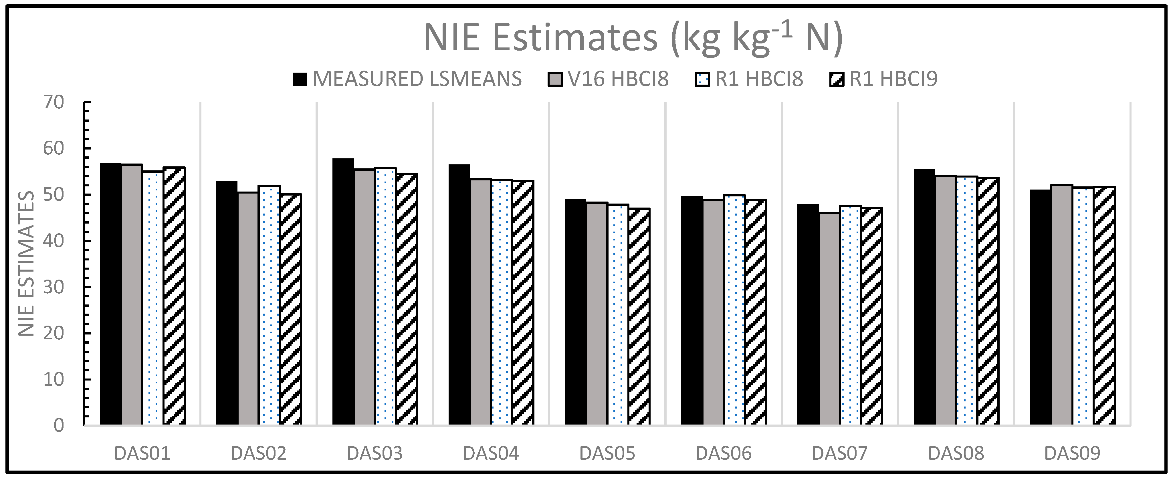
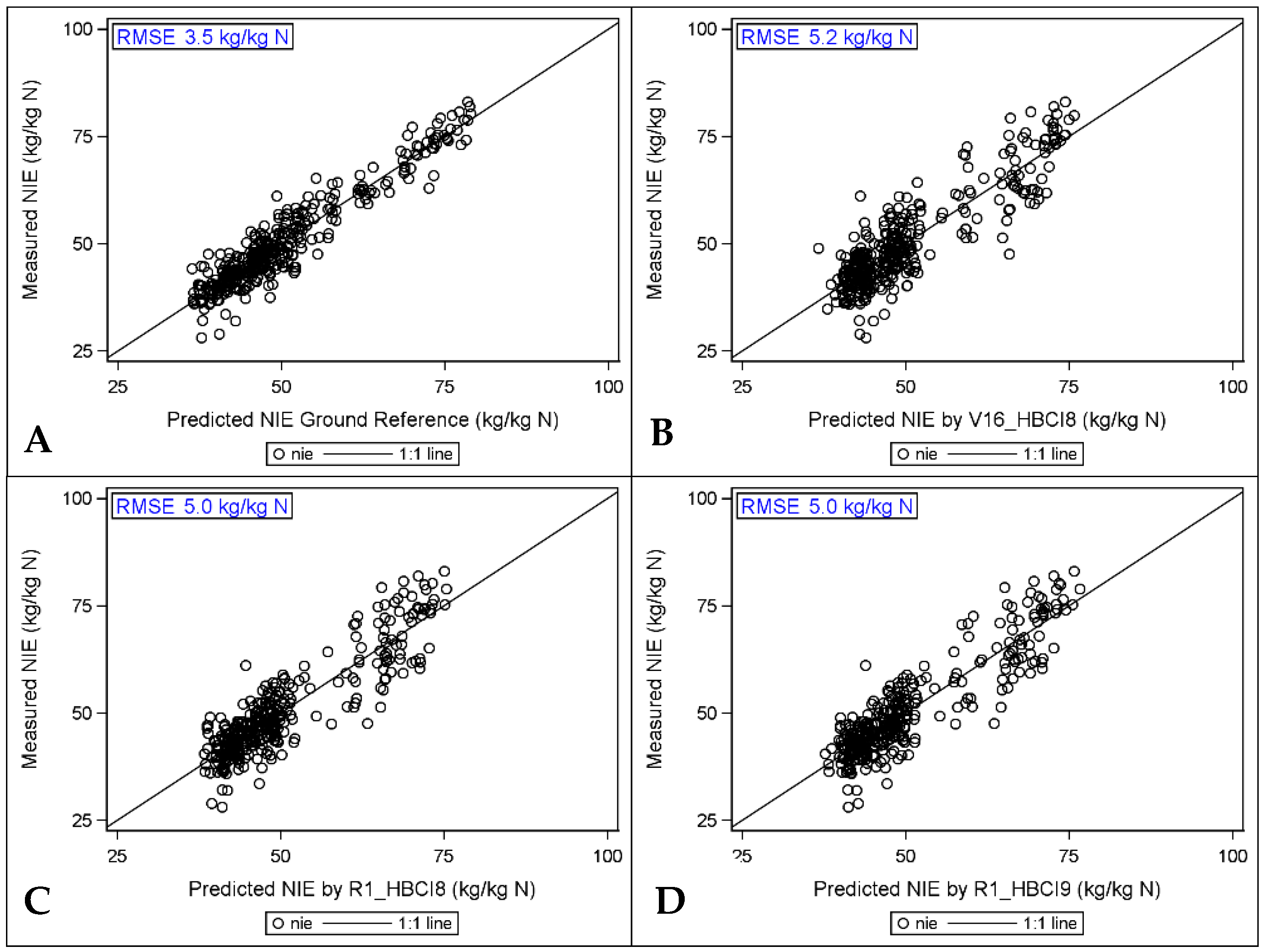
The LS means chart (Figure 7) showed that the three HSI models often underestimated the hybrid mean values. The smallest differences between estimated and measured values were evident for HBCI8 at both imaging dates. The measured vs. predicted plots shown in Figure 8 showed a similar scatter pattern around the 1:1 line for all three models. All three also had only slightly more scatter than the ground reference model. The three HSI models provided the ability to separate the best hybrids in NIE (DAS01 and DAS03) from the bottom performing hybrids of DAS05 and DAS07 based on mid-season imaging data. This suggests that these HSI extracted from imaging during the growing season could be deployed prior to the end of the growing season in order to facilitate decision-based selection as part of an early stage breeding program.
The set of indices discussed here, HBCI8 and HBCI9, are classified as hyperspectral biochemical indices (HBCI) designed for studying pigments such as carotenoids and chlorophyll [27]. Both HSI contain one band (550 nm) which increases in reflectance as chlorophyll levels decrease [70]. Accordingly, our results suggest that mid-season chlorophyll was a stronger factor in NIE prediction by HSI than other biophysical components of biomass or canopy structure.
End-season NIE hybrid predictions were remarkably accurate based on HSI extracted from mid-season imaging. Further studies are recommended to validate this finding for other genotypes and environments. Additionally, the HSI identified as predictive of NIE (HBCI8 and HBCI9) were based on the green portion of the electromagnetic spectrum or the ratio of green:blue (G:B). No other G:G or G:B indices were investigated here. Similar indices may be more accurate predictors of NIE; thus, we recommend further research into similar indices.
3.6. Comparison of High to Low Spatial Resolution HSI
The image data obtained in 2017 at ACRE which had extremely high resolution (4 cm pixels) were resampled to match the 2014 50 cm pixel data. The effect of this downsampling is examined in this section for the five HSI identified as predicting hybrid differences for NCE and NIE. The resolution effect on pN was not analyzed since the HSI did not detect hybrid differences in pN for the global dataset.
The analysis by each HSI (HBCI8, HBCI9, HBSI2, HBSI2 at R1 and HBCI8 at V16) showed that the low- and-high resolution data were highly positively correlated based on Pearson correlation coefficients (r ≥ 0.97, n = 104). However, the matched pairs t-tests, both by plot and across plots, indicated HSI values were significantly different at the two resolutions. For all HSI, resampling the high-resolution images resulted in significantly increased index values for the low-resolution images, likely due to mixed pixel effects associated with shadows and soil. These differences decreased at greater HSI values. This result confirms the theoretical analysis of the effect of spatial resolution on NDVI by [74] who found that NDVI-low resolution is greater than NDVI-high resolution. However, in their analysis the largest difference was found at moderate and low vegetation levels (20–50%) and darker soils [74]. These researchers found less difference in the two resolutions as vegetation proportion increased or with high red reflectance soils. In our research, the HSI were calculated at V16/18 or R1/2, by which time the canopy had already closed; thus, high vegetation levels and little visible soil precluded a similar analysis. Overall, our findings indicated that the correlations between HSI and N parameters (NCE or NIE) did not change in a consistent pattern as the resolution of the maize fields decreased with downsampling.
Impact of Resolution Difference on Rankings
Upon detection of the statistically significant effect of resampling and downgrading the 2017 image data, an analysis was conducted to determine the effect of resampling on hybrid rankings from the models themselves. For NCE all HSI, regardless of time-point or resolution, were unable to detect the hybrid differences evident in the measured data at ACRE (Table 10). The NCE model estimates were quite similar to the ground reference data, often correctly identifying the hybrid with the lowest and highest NCE numerical values. However, these differences were not statistically significant. Since the HSI were able to determine some statistical differences in hybrids for NCE when using all three site-years, this result suggests that the models based on imaging need larger quantities of data—more than what were available within our single location at ACRE.
A similar analysis was conducted using the imaging data at ACRE for NIE prediction. We found slight statistical differences in hybrid rankings only for V16 HBCI8 (Table 11). The other two HSI did not show differences in hybrid rankings between the high- and low-resolution data. Overall, there was no consistent effect from the change in spatial resolution for NIE. Nevertheless, none of the image data (high or low resolution) were able to differentiate the hybrids as with the measured data, similar to the NCE findings. Consequently, the effect of resolution change on hybrids could not be fully evaluated.
The significant differences in the index values with no change in the correlations between HSI and N parameters, in addition to the inability to differentiate hybrids with either high or low resolution, are ambiguous results. The lack of corroboration of our results with other research may be due to the fact that these images were acquired after canopy closure and resolution tends to have a greater impact earlier in the season. Additional investigation into this timing aspect is needed.
4. Conclusions
In this study we evaluated 20 HSI at two time-points (V16 and R1) across three site-years for detecting hybrid differences and predicting pN at R6, NCE at R6 and NIE. Our experiment encompassed strikingly different environments (California valley basin vs. Eastern Cornbelt) for five to nine common hybrids. The multiple N rates and plant densities in each environment resulted in a moderate range of NCE and NIE values at maturity.
In these experiments, we found two HSI at R1, a structural index and a red-edge index (HBSI2682,910 and HREI16705,910), were well-suited for predicting plant N concentration at R6, but not for identification and separation of hybrid differences. For NCE, we identified two structural HSI at R1 (HBSI1682,855 and HBSI2682,910) to be predictive of NCE and hybrid differences. Both HSI identified the hybrid with the highest NCE and the two hybrids with the lowest NCE. Finally, two biochemical HSIs (HBCI8515,550 at V16 and R1 and HBCI9490,550 at R1) were predictive of NIE, the amount of grain yield per unit plant N. These HSI also detected significant hybrid differences similar to those identified by the ground reference data. The top two NIE hybrids were differentiated from the three lowest ranking hybrids. Overall, our findings indicated a greater ability to accurately predict NIE than NCE and the weakest predictability for pN. To our knowledge, this is the first effort using vegetation indices from hyperspectral imaging in mid-season maize production for predicting end-season NCE and NIE.
In the global analysis across all three site-years, the low resolution (50 cm) image data were adequate for detecting hybrid differences. However, our results from the resolution analysis indicated that, while index values changed, the effect of resolution change on hybrid differentiation was not evident, since hybrid differences were not apparent at either high (4 cm) or low (50 cm) pixel resolution. We hypothesized these ambiguous results were due to the limited dataset.
The HSI newly identified as predictive of NCE and NIE correctly ranked the best hybrids early in the season (at V16 or R1), thus enabling opportunities for reducing hand sampling and field data collection of hybrids with lower N efficiencies. We hope these HSI, after additional validation, can be applied directly for the foundational work needed in breeding for N efficiency in maize. Implementation of these HSI or other remote sensing methods into routine breeding efforts can only improve and hasten our understanding and development of N-efficient maize hybrids.
Supplementary Materials
The following supporting information can be downloaded at: https://www.mdpi.com/article/10.3390/rs14071721/s1, Figure S1. Experiment site locations in Woodland, California (yellow location pin marked as “Rominger plots”) and West Lafayette, Indiana (yellow location pin marked as “ACRE plots”), Table S1. Monthly weather averages (precip = precipitation; temp = temperature; deg = degrees), Table S2. Soil nutrient characteristics, Table S3. Mixed model analysis of treatment effects and interactions on physiological characteristics across 3 site-years (α = 0.10), Table S4. Least square mean estimates of plant biomass at R6 (TDM), and N content (TNC) at V12, R1 and R6 for the main fixed effects of hybrid (H), nitrogen (N), and plant density (PD). References [75,76,77,78] are cited in the supplementary materials.
Author Contributions
Conceptualization, M.B.O. and T.J.V.; methodology, M.B.O., M.M.C. and T.J.V.; software, M.B.O.; validation, M.B.O. and M.M.C.; formal analysis, M.B.O.; investigation, M.B.O.; resources, M.B.O., M.M.C. and T.J.V.; data curation, M.B.O.; writing—original draft preparation, M.B.O.; writing—review and editing, M.B.O., M.M.C. and T.J.V.; visualization, M.B.O.; supervision, M.M.C. and T.J.V.; project administration, T.J.V.; funding acquisition, M.B.O. and T.J.V. All authors have read and agreed to the published version of the manuscript.
Funding
This research was funded by Dow AgroSciences LLC and Corteva Agriscience™.
Institutional Review Board Statement
Not applicable.
Informed Consent Statement
Not applicable.
Data Availability Statement
Remote sensing data are currently available via correspondence with the authors. Data will be archived at Purdue University for at least 5 years.
Acknowledgments
We would like to acknowledge all field station support, especially that at Gorman and Rominger, which was instrumental to the generation of the data used in this research.
Conflicts of Interest
The authors declare no conflict of interest. The funders had no role in the analyses or interpretation of data, in the writing of the manuscript, or in the decision to publish the results.
References
- Ribaudo, M.; Hansen, L.; Livingston, M.; Mosheim, R.; Williamson, J.; Delgado, J. Nitrogen in agricultural systems: Implications for conservation policy. USDA-ERS Econ. Res. Rep. 2011, 127, 89. [Google Scholar] [CrossRef] [Green Version]
- Mueller, S.M.; Messina, C.D.; Vyn, T.J. Simultaneous gains in grain yield and nitrogen efficiency over 70 years of maize genetic improvement. Sci. Rep. 2019, 9, 9095. [Google Scholar] [CrossRef] [PubMed] [Green Version]
- Doering, O.; Galloway, J.; Theis, T.; Aneja, V.; Boyer, E.; Cassman, K.; Cowling, E.; Dickerson, R.; Herz, W.; Hey, D. Reactive Nitrogen in the United States: An Analysis of Inputs, Flows, Consequences, and Management Options; Board, E.S.A., Ed.; United States Environmental Protection Agency: Washington, DC, USA, 2011.
- Chen, K.; Vyn, T.J. Post-silking factor consequences for N efficiency changes over 38 years of commercial maize hybrids. Front. Plant Sci. 2017, 8, 1737. [Google Scholar] [CrossRef] [PubMed] [Green Version]
- Ciampitti, I.A.; Vyn, T.J. Physiological perspectives of changes over time in maize yield dependency on nitrogen uptake and associated nitrogen efficiencies: A review. Field Crops Res. 2012, 133, 48–67. [Google Scholar] [CrossRef]
- DeBruin, J.L.; Schussler, J.R.; Mo, H.; Cooper, M. Grain yield and nitrogen accumulation in maize hybrids released during 1934 to 2013 in the US Midwest. Crop Sci. 2017, 57, 1431–1446. [Google Scholar] [CrossRef]
- Moose, S.; Below, F.E. Biotechnology approaches to improving maize nitrogen use efficiency. In Molecular Genetic Approaches to Maize Improvement; Kriz, A.L., Larkins, B.A., Eds.; Springer: Berlin/Heidelberg, Germany, 2009; pp. 65–77. [Google Scholar]
- Moll, R.H.; Kamprath, E.J.; Jackson, W.A. Analysis and interpretation of factors which contribute to efficiency of nitrogen utilization. Agron. J. 1982, 74, 562–564. [Google Scholar] [CrossRef]
- Shrawat, A.; Zayed, A.; Lightfoot, D.A. (Eds.) Engineering Nitrogen Utilization in Crop Plants; Springer International Publishing: Berlin/Heidelberg, Germany, 2018. [Google Scholar]
- Salvagiotti, F.; Castellarín, J.M.; Miralles, D.J.; Pedrol, H.M. Sulfur fertilization improves nitrogen use efficiency in wheat by increasing nitrogen uptake. Field Crops Res. 2009, 113, 170–177. [Google Scholar] [CrossRef]
- Ciampitti, I.A.; Vyn, T.J. A comprehensive study of plant density consequences on nitrogen uptake dynamics of maize plants from vegetative to reproductive stages. Field Crops Res. 2011, 121, 2–18. [Google Scholar] [CrossRef]
- Gastal, F.; Lemaire, G.; Durand, J.-L.; Louarn, G. Quantifying crop responses to nitrogen and avenues to improve nitrogen-use efficiency. In Crop Physiology, 2nd ed.; Academic Press: Cambridge, MA, USA, 2015; pp. 161–206. [Google Scholar]
- Muñoz-Huerta, R.F.; Guevara-Gonzalez, R.G.; Contreras-Medina, L.M.; Torres-Pacheco, I.; Prado-Olivarez, J.; Ocampo-Velazquez, R.V. A review of methods for sensing the nitrogen status in plants: Advantages, disadvantages and recent advances. Sensors 2013, 13, 10823–10843. [Google Scholar] [CrossRef] [PubMed]
- Unkovich, M.; Herridge, D.; Peoples, M.; Cadisch, G.; Boddey, B.; Giller, K.; Alves, B.; Chalk, P. Measuring Plant-Associated Nitrogen Fixation in Agricultural Systems; Australian Centre for International Agricultural Research (ACIAR): Canberra, Australia, 2008.
- Zhao, D.; Raja Reddy, K.; Kakani, V.G.; Read, J.J.; Carter, G.A. Corn (Zea mays L.) growth, leaf pigment concentration, photosynthesis and leaf hyperspectral reflectance properties as affected by nitrogen supply. Plant Soil 2003, 257, 205–218. [Google Scholar] [CrossRef]
- Araus, J.L.; Cairns, J.E. Field high-throughput phenotyping: The new crop breeding frontier. Trends Plant Sci. 2014, 19, 52–61. [Google Scholar] [CrossRef] [PubMed]
- Cobb, J.N.; DeClerck, G.; Greenberg, A.; Clark, R.; McCouch, S. Next-generation phenotyping: Requirements and strategies for enhancing our understanding of genotype–phenotype relationships and its relevance to crop improvement. Theor. Appl. Genet. 2013, 126, 867–887. [Google Scholar] [CrossRef] [Green Version]
- Jin, X.; Zarco-Tejada, P.; Schmidhalter, U.; Reynolds, M.P.; Hawkesford, M.J.; Varshney, R.K.; Yang, T.; Nie, C.; Li, Z.; Ming, B. High-throughput estimation of crop traits: A review of ground and aerial phenotyping platforms. IEEE Geosci. Remote Sens. Mag. 2020, 9, 200–231. [Google Scholar] [CrossRef]
- Nguyen, G.N.; Kant, S. Improving nitrogen use efficiency in plants: Effective phenotyping in conjunction with agronomic and genetic approaches. Funct. Plant Biol. 2018, 45, 606. [Google Scholar] [CrossRef] [PubMed]
- Rodrigues Junior, F.A.; Ortiz-Monasterio, I.; Zarco-Tejada, P.J.; Ammar, K.; Gérard, B. Using precision agriculture and remote sensing techniques to improve genotype selection in a breeding program. In Proceedings of the 12th International Conference on Precision Agriculture (ICPA), Sacramento, CA, USA, 20–23 July 2014. [Google Scholar]
- White, J.W.; Andrade-Sanchez, P.; Gore, M.A.; Bronson, K.F.; Coffelt, T.A.; Conley, M.M.; Feldmann, K.A.; French, A.N.; Heun, J.T.; Hunsaker, D.J.; et al. Field-based phenomics for plant genetics research. Field Crops Res. 2012, 133, 101–112. [Google Scholar] [CrossRef]
- Lillesand, T.; Kiefer, R.W.; Chipman, J. Remote Sensing and Image Interpretation; John Wiley & Sons: Hoboken, NJ, USA, 2014. [Google Scholar]
- Campbell, J.B.; Wynne, R.H. Introduction to Remote Sensing; Guilford Press: New York, NY, USA, 2011. [Google Scholar]
- Mulla, D.J. Twenty five years of remote sensing in precision agriculture: Key advances and remaining knowledge gaps. Biosyst. Eng. 2013, 114, 358–371. [Google Scholar] [CrossRef]
- Goel, P.K.; Prasher, S.O.; Landry, J.A.; Patel, R.M.; Viau, A.A.; Miller, J.R. Estimation of crop biophysical parameters through airborne and field hyperspectral remote sensing. Trans. ASAE 2003, 46, 1235–1246. [Google Scholar]
- Osborne, S.L.; Schepers, J.S.; Francis, D.D.; Schlemmer, M.R. Use of spectral radiance to estimate in-season biomass and grain yield in nitrogen- and water- stressed corn. Crop Sci. 2002, 42, 165–171. [Google Scholar]
- Thenkabail, P.S.; Gumma, M.K.; Teluguntla, P.; Mohammed, I.A. Hyperspectral remote sensing of vegetation and agricultural crops. Photogramm. Eng. Remote Sens. 2014, 80, 697–723. [Google Scholar]
- Thenkabail, P.S.; Smith, R.B.; De Pauw, E. Hyperspectral vegetation indices and their relationships with agricultural crop characteristics. Remote Sens. Environ. 2000, 71, 158–182. [Google Scholar] [CrossRef]
- Blackmer, T.M.; Schepers, J.S.; Varvel, G.E.; Walter-Shea, E.A. Nitrogen deficiency detection using reflected shortwave radiation from irrigated corn canopies. Agron. J. 1996, 88, 1–5. [Google Scholar] [CrossRef] [Green Version]
- Elsayed, S.; Darwish, W. Hyperspectral remote sensing to assess the water status, biomass, and yield of maize cultivars under salinity and water stress. Bragantia 2017, 76, 62–72. [Google Scholar] [CrossRef] [Green Version]
- Campbell, P.; Middleton, E.; McMurtrey, J.; Chappelle, E. Assessment of vegetation stress using reflectance or fluorescence measurements. J. Environ. Qual. 2007, 36, 832–845. [Google Scholar] [CrossRef]
- Osborne, S.L.; Schepers, J.S.; Francis, D.D.; Schlemmer, M.R. Detection of phosphorus and nitrogen deficiencies in corn using spectral radiance measurements. Agron. J. 2002, 94, 1215–1221. [Google Scholar] [CrossRef] [Green Version]
- Schlemmer, M.R.; Francis, D.D.; Shanahan, J.; Schepers, J.S. Remotely measuring chlorophyll content in corn leaves with differing nitrogen levels and relative water content. Agron. J. 2005, 97, 106–112. [Google Scholar] [CrossRef] [Green Version]
- Thenkabail, P.S.; Lyon, J.G.; Huete, A. Hyperspectral Remote Sensing of Vegetation; CRC Press: Boca Raton, FL, USA, 2012. [Google Scholar]
- Midwestern Regional Climate Center. Available online: https://mrcc.illinois.edu/CLIMATE/ (accessed on 8 June 2019).
- Indiana State Climate Office. Available online: www.iclimate.org (accessed on 2 December 2017).
- Miller, R.O.; Gavlak, R.; Horneck, D. Soil, Plant and Water Reference Methods for the Western Region; WCC-103 Publication: Fort Collins, CO, USA, 2013; p. 156. [Google Scholar]
- NCERA-13; Eliason, R.; Goos, R.J.; Hoskins, B. Recommended Chemical Soil Test Procedures for the North Central Region; NCERA-13, Ed.; Missouri Agricultural Experiment Station: Columbia, MO, USA, 2015; p. 76. [Google Scholar]
- US EPA. Standard method 350.1: Nitrogen, ammonia (colorimetric, automated phenate). In Methods for the Determination of Inorganic Substances in Environmental Samples; Office of Research and Development, US EPA: Cincinnati, OH, USA, 1993. [Google Scholar]
- US EPA. Method 353.2: Determination of Nitrate—Nitrite Nitrogen by Automated Colorimetry, Revision 2.0; O’Dell, J., Ed.; Environmental Monitoring Systems Laboratory: Cincinnati, OH, USA, 1993.
- Dellavalle Laboratory Inc. Soil Interpretation Report; Kasapligil, D., Ed.; Dellavalle Laboratory, Inc.: Davis, CA, USA, 2014. [Google Scholar]
- Vitosh, M.; Johnson, J.; Mengel, D. Tri-State Fertilizer Recommendations for Corn, Soybeans, Wheat and Alfalfa; Michigan State University Extension: East Lansing, MI, USA, 1995. [Google Scholar]
- Rouse, J.W.J.; Haas, R.H.; Schell, J.A.; Deering, D.W.; Harlan, J.C. Monitoring the Vernal Advancment and Retrogradation (Greenwave Effect) of Natural Vegetation; Texas A&M University Remote Sensing Center: College Station, TX, USA, 1974. [Google Scholar]
- Qi, J.; Chehbouni, A.; Huete, A.; Kerr, Y.; Sorooshian, S. A modified soil adjusted vegetation index. Remote Sens. Environ. 1994, 48, 119–126. [Google Scholar] [CrossRef]
- Chen, P.-F.; Nicolas, T.; Wang, J.-H.; Philippe, V.; Huang, W.-J.; Li, B.-G. New index for crop canopy fresh biomass estimation. Spectrosc. Spectr. Anal. 2010, 30, 512–517. [Google Scholar]
- Merzlyak, M.N.; Gitelson, A.A.; Chivkunova, O.B.; Rakitin, V.Y. Non-destructive optical detection of pigment changes during leaf senescence and fruit ripening. Physiol. Plant. 1999, 106, 135–141. [Google Scholar] [CrossRef] [Green Version]
- Daughtry, C.S.T.; Walthall, C.L.; Kim, M.S.; Brown de Colstoun, E.; McMurtrey, J.E., III. Estimating corn leaf chlorophyll concentration from leaf and canopy reflectance. Remote Sens. Environ. 2000, 74, 229–239. [Google Scholar] [CrossRef]
- Chen, P.; Haboudane, D.; Tremblay, N.; Wang, J.; Vigneault, P.; Li, B. New spectral indicator assessing the efficiency of crop nitrogen treatment in corn and wheat. Remote Sens. Environ. 2010, 114, 1987–1997. [Google Scholar] [CrossRef]
- Xue, L.; Cao, W.; Luo, W.; Dai, T.; Zhu, Y. Monitoring leaf nitrogen status in rice with canopy spectral reflectance. Agron. J. 2004, 96, 135–142. [Google Scholar] [CrossRef]
- Kim, M.S.; Daughtry, C.; Chappelle, E.; McMurtrey, J.; Walthall, C. The use of high spectral resolution bands for estimating absorbed photosynthetically active radiation (A par). In Proceedings of the 6th Symposium on Physical Measurements and Signatures in Remote Sensing, Val D’Isere, France, 17–24 January 1994; pp. 299–306. [Google Scholar]
- Kim, M.S. The Use of Narrow Spectral Bands for Improving Remote Sensing Estimations of Fractionally Absorbed Photosynthetically Active Radiation. In Department of Geography; University of Maryland: College Park, MD, USA, 1994. [Google Scholar]
- Rondeaux, G.; Steven, M.; Baret, F. Optimization of soil-adjusted vegetation indices. Remote Sens. Environ. 1996, 55, 95–107. [Google Scholar] [CrossRef]
- Haboudane, D.; Miller, J.R.; Tremblay, N.; Zarco-Tejada, P.J.; Dextraze, L. Integrated narrow-band vegetation indices for prediction of crop chlorophyll content for application to precision agriculture. Remote Sens. Environ. 2002, 81, 416–426. [Google Scholar] [CrossRef]
- Barnes, E.; Clarke, T.; Richards, S.; Colaizzi, P.; Haberland, J.; Kostrzewski, M.; Waller, P.; Choi, C.; Riley, E.; Thompson, T. Coincident detection of crop water stress, nitrogen status and canopy density using ground based multispectral data. In Proceedings of the Fifth International Conference on Precision Agriculture, Bloomington, MN, USA, 16–19 July 2000. [Google Scholar]
- Gitelson, A.A.; Gritz, Y.; Merzlyak, M.N. Relationships between leaf chlorophyll content and spectral reflectance and algorithms for non-destructive chlorophyll assessment in higher plant leaves. J. Plant Physiol. 2003, 160, 271–282. [Google Scholar] [CrossRef] [PubMed]
- Montgomery, D.C.; Peck, E.A.; Vining, G.G. Introduction to Linear Regression Analysis, 5th ed.; John Wiley & Sons: Hoboken, NJ, USA, 2012; Volume 821. [Google Scholar]
- Bundy, L.; Carter, P. Corn hybrid response to nitrogen fertilization in the northern corn belt. J. Prod. Agric. 1988, 1, 99–104. [Google Scholar] [CrossRef] [Green Version]
- Jeschke, M.; DeBruin, J. Corn hybrid response to nitrogen fertilizer. In Crop Insights; DuPont Pioneer Agronomy Sciences: Johnston, Hungary, 2016; pp. 1–7. [Google Scholar]
- Chevalier, P.; Schrader, L. Genotypic differences in nitrate absorption and partitioning of N among plant parts in maize. Crop Sci. 1977, 17, 897–901. [Google Scholar] [CrossRef]
- Sadras, V.O.; Calderini, D.F. Crop Physiology: Applications for Genetic Improvement and Agronomy, 2nd ed.; Academic Press: Cambridge, MA, USA, 2015. [Google Scholar]
- Plénet, D.; Lemaire, G. Relationships between dynamics of nitrogen uptake and dry matter accumulation in maize crops. Determination of critical N concentration. Plant Soil 2000, 216, 65–82. [Google Scholar] [CrossRef]
- Haegele, J.W.; Cook, K.A.; Nichols, D.M.; Below, F.E. Changes in nitrogen use traits associated with genetic improvement for grain yield of maize hybrids released in different decades. Crop Sci. 2013, 53, 1256. [Google Scholar] [CrossRef] [Green Version]
- D’Andrea, K.E.; Otegui, M.E.; Cirilo, A.G.; Eyhérabide, G.H. Ecophysiological traits in maize hybrids and their parental inbred lines: Phenotyping of responses to contrasting nitrogen supply levels. Field Crops Res. 2009, 114, 147–158. [Google Scholar] [CrossRef]
- Schlemmer, M.; Gitelson, A.; Schepers, J.; Ferguson, R.; Peng, Y.; Shanahan, J.; Rundquist, D. Remote estimation of nitrogen and chlorophyll contents in maize at leaf and canopy levels. Int. J. Appl. Earth Obs. Geoinf. 2013, 25, 47–54. [Google Scholar] [CrossRef] [Green Version]
- Zhao, B.; Duan, A.; Ata-Ul-Karim, S.T.; Liu, Z.; Chen, Z.; Gong, Z.; Zhang, J.; Xiao, J.; Liu, Z.; Qin, A.; et al. Exploring new spectral bands and vegetation indices for estimating nitrogen nutrition index of summer maize. Eur. J. Agron. 2018, 93, 113–125. [Google Scholar] [CrossRef]
- Haboudane, D.; Tremblay, N.; Miller, J.R.; Vigneault, P. Remote estimation of crop chlorophyll content using spectral indices derived From hyperspectral data. IEEE Trans. Geosci. Remote Sens. 2008, 46, 423–437. [Google Scholar] [CrossRef]
- Hunt Jr, E.R.; Doraiswamy, P.C.; McMurtrey, J.E.; Daughtry, C.S.; Perry, E.M.; Akhmedov, B. A visible band index for remote sensing leaf chlorophyll content at the canopy scale. Int. J. Appl. Earth Obs. Geoinf. 2013, 21, 103–112. [Google Scholar] [CrossRef] [Green Version]
- Zhou, K.; Cheng, T.; Zhu, Y.; Cao, W.; Ustin, S.L.; Zheng, H.; Yao, X.; Tian, Y. Assessing the impact of spatial resolution on the estimation of leaf nitrogen concentration over the full season of paddy rice using near-surface imaging spectroscopy data. Front. Plant Sci. 2018, 9, 964. [Google Scholar] [CrossRef] [Green Version]
- Boomsma, C.R.; Santini, J.B.; Tollenaar, M.; Vyn, T.J. Maize morphophysiological responses to intense crowding and low nitrogen availability: An analysis and review. Agron. J. 2009, 101, 1426. [Google Scholar] [CrossRef] [Green Version]
- Buschmann, C.; Nagel, E. In vivo spectroscopy and internal optics of leaves as basis for remote sensing of vegetation. Int. J. Remote Sens. 1993, 14, 711–722. [Google Scholar] [CrossRef]
- Thenkabail, P.S.; Smith, R.B.; De Pauw, E. Evaluation of narrowband and broadband vegetation indices for determining optimal hyperspectral wavebands for agricultural crop characterization. Photogramm. Eng. Remote Sens. 2002, 68, 607–622. [Google Scholar]
- Blackburn, G.A. Quantifying chlorophylls and carotenoids at leaf and canopy scales: An evaluation of some hyperspectral approaches. Remote Sens. Environ. 1998, 66, 273–285. [Google Scholar] [CrossRef]
- Goel, N.S.; Qin, W. Influences of canopy architecture on relationships between various vegetation indices and LAI and Fpar: A computer simulation. Remote Sens. Rev. 1994, 10, 309–347. [Google Scholar] [CrossRef]
- Jiang, Z.; Chen, Y.; Li, J.; Dou, W. The impact of spatial resolution on NDVI over heterogeneous surface. In Proceedings of the 2005 IEEE International Geoscience and Remote Sensing Symposium, 2005, IGARSS’05, Seoul, Korea, 29 July 2005; pp. 1310–1313. [Google Scholar]
- Google Data SIO, NOAA, U.S. Navy, NGA, GEBCO Landsat/Copernicus INEGI Data LDEO-Columbia, NSF, and N. IBCAO. Google Earth 2022. Available online: earth.google.com (accessed on 11 March 2022).
- Chenu, K. Characterizing the crop environment–nature, significance and applications. In Crop Physiology; Elsevier: Amsterdam, The Netherlands, 2015; pp. 321–348. [Google Scholar]
- Connor, D.J.; Loomis, R.S.; Cassman, K.G. Crop Ecology: Productivity and Management in Agricultural Systems; Cambridge University Press: Cambridge, UK, 2011. [Google Scholar]
- Schepers, J.S.; Raun, W. (Eds.) Nitrogen in Agricultural Systems; ASA-CSSA-SSSA: Madison, WI, USA, 2008. [Google Scholar]
Figure 1.
Decision tree used for selecting the best HSI models.

Figure 2.
Pearson correlation coefficients (r) by V16/18 or R1/2 HSI for pN at R6, NCE at R6, and NIE at R6 for each location. Blue = ACRE (IN), Red = Gorman (CA), and Yellow = Rominger (CA). Dotted lines at |0.3| are for reference only. Green boxes highlight some of the strongest or more consistent correlations.

Figure 3.
Least square means estimates of N concentration (pN) (%) by hybrid for the ground reference model, HBSI2 and HREI16 at R1 models.
Figure 3.
Least square means estimates of N concentration (pN) (%) by hybrid for the ground reference model, HBSI2 and HREI16 at R1 models.

Figure 4.
Predicted vs. actual (measured) estimates of N concentration (pN) (%) with RMSE for each plot. Black line is 45° reference line (1:1 line). (A) Ground reference mixed model; (B) R1 HBSI2; (C) R1 HREI16 models.
Figure 4.
Predicted vs. actual (measured) estimates of N concentration (pN) (%) with RMSE for each plot. Black line is 45° reference line (1:1 line). (A) Ground reference mixed model; (B) R1 HBSI2; (C) R1 HREI16 models.

Figure 5.
Least square means estimates of NCE by hybrid based on measured or HSI models.

Figure 6.
Predicted vs. actual (measured) estimates of NCE with RMSE for each plot. The black line is the 45° reference line (1:1 line). (A) Ground reference mixed model; (B) R1 HBSI1 model; (C) R1 HBSI2 model.
Figure 6.
Predicted vs. actual (measured) estimates of NCE with RMSE for each plot. The black line is the 45° reference line (1:1 line). (A) Ground reference mixed model; (B) R1 HBSI1 model; (C) R1 HBSI2 model.

Figure 7.
Least square means estimates of NIE by hybrid based on measured or HSI models.

Figure 8.
Predicted vs. actual (measured) estimates of NIE with RMSE for each plot. The black line is the 45° reference line (1:1 line). (A) Ground reference mixed model; (B) V16 HBCI8 model; (C) R1 HBCI8 model; (D) R1 HBCI9 model.
Figure 8.
Predicted vs. actual (measured) estimates of NIE with RMSE for each plot. The black line is the 45° reference line (1:1 line). (A) Ground reference mixed model; (B) V16 HBCI8 model; (C) R1 HBCI8 model; (D) R1 HBCI9 model.


Table 1.
Experiment design with sampling and imaging dates.
| Year | Location | Planting Date | Harvest Date | Final Plant Density (Plants ha−1) | Plot Size (w × l) | N Trt (kg N ha−1) (Appl Time) | BM Sampling Stages and Dates | Hybrids | RS Dates |
|---|---|---|---|---|---|---|---|---|---|
| 2014 | Woodland, CA (Gorman) | 5/14 | 9/17 | 65,000 95,000 | 4.6 m × 12 m (6 rows) | 0 56 (V4) 224 (pre, V4 and V8) | V12 (6/25) V18 (7/14) R2 (7/22) R6 (9/17) | DAS01 DAS02 DAS03 DAS04 DAS05 DAS06 DAS07 DAS08 DAS09 | V18 (7/11) R1 (7/24) |
| Woodland, CA (Rominger) | 5/27 | 10/2 | V12 (7/7) R1 (7/25) R6 (10/2) | V18 (7/11) R2 (7/24) | |||||
| 2017 | West Lafayette, IN (ACRE) | 5/17 | 10/17 | 69,100 99,600 | 3 m × 15 m (4 rows) | 0 56 (V5) 224 (V5) | V12 (7/12) R1 (7/24) R6 (10/5) | DAS02 DAS03 DAS04 DAS05 DAS09 | V5 (6/16) V8 (6/27) V16/17 (7/18) R1 (7/25) R3/R4 (8/20) R5 (9/8) R5/R6 (9/22) |
Note: w = wide; l = long; Trt = treatment; Appl = application; BM = Biomass; pre = pre-plant; RS = remote sensing.
Table 2.
Soil N testing results.
| N Levels (mg kg−1) | ||||||||||
|---|---|---|---|---|---|---|---|---|---|---|
| Sampling Time | Pre-Plant | V3 | V12 | |||||||
| Sampling Depth (cm) | Gor NO3− N LN | Gor NO3− N HN | Rom NO3− N LN | Rom NO3− N HN | ACRE NO3− N LN | ACRE NH4+ N LN | ACRE NO3− N LN | ACRE NO3− N HN | ACRE NH4+ N LN | ACRE NH4+ N HN |
| 0–15 | 19 | 24 | 9 | 10 | 14 | 4 | 2 | 3 | 6 | 6 |
| 15–30 | 29 | 25 | 9 | 12 | ||||||
| 30–60 | na | na | na | na | 11 | 3 | 2 | 4 | 4 | 4 |
Note: Gor = Gorman; Rom = Rominger; LN = Low N treatment plots; HN = High N treatment plots; na = not available.
Table 3.
Summary of hyperspectral indices (HSI) evaluated.
| Category | Spectral Index | Equation | Reference |
|---|---|---|---|
| Biomass | NDVI | (R800 − R670)/(R800 + R670) | [43] |
| MSAVI | 0.5 × (2 × R800 + 1 − (sqrt((2 × R800 +1)2 − 8 × (R800 − R670))) | [44] | |
| RTVI | (100 × (R750 − R730) − (10 × (R750 − R550)) × sqrt(R700/R670)) | [45] | |
| Grain Yield/Structural | PSRI | (R678 − R500)/R750 | [46] |
| HBSI1 | (R855 − R682)/(R855 + R682) | [27,34] | |
| HBSI2 | (R910 − R682)/(R910 + R682) | ||
| HBSI3 | (R550 − R682)/(R550 + R682) | ||
| Chlorophyll or N Concentration | HBCI8 | (R550 − R515)/(R550 + R515) | [27,34] |
| HBCI9 | (R550 − R490)/(R550 + R490) | ||
| HBCI10 | (R720 − R550)/(R720 + R550) | ||
| MCARI | ((R700 − R670) − 0.2 × (R700 − R550)) × (R700/R670) | [47] | |
| DCNI | (R720 − R700)/(R700 − R670)/(R720 − R670 + 0.03) | [48] | |
| RVI II | R810/R560 | [49] | |
| TCARI | 3 × ((R700 − R670) − 0.2 × (R700 − R550) × (R700/R670)) | [50,51] | |
| OSAVI | ((1 + 0.16) × (R800 − R670))/(R800 + R670 + 0.16) | [52] | |
| TCARI/OSAVI | TCARI/OSAVI | [53] | |
| Plant Stress | HREI15 | (R855 − R720)/(R855 + R720) | [27,34] |
| HREI16 | (R910 − R705)/(R910 + R705) | [27,34] | |
| NDRE | (R790 − R720)/(R790 + R720) | [54] | |
| CIRE | (R750 − R800)/(R695 − R740) − 1 | [55] |
Note: NDVI = Normalized Difference Vegetation Index; MSAVI = Modified Soil Adjusted Vegetation Index; RTVI = Red-edge Triangular Vegetation Index; PSRI = Plant Senescence Reflectance Index; HBSI = Hyperspectral Biomass and Structural Index; HBCI = Hyperspectral Biochemical Index; MCARI = Modified Chlorophyll Absorption Reflectance Index; DCNI = Double-peak Canopy Nitrogen Index; RVI II = Ratio Vegetation Index II; TCARI = Transformed Chlorophyll Absorption Ratio; OSAVI = Optimized Soil Adjusted Vegetation Index; HREI = Hyperspectral Red Edge Index; NDRE = Normalized Difference Red Edge; CIRE = Chlorophyll Index Red Edge.
Table 4.
Least square mean estimates of pN at R6 and grain yield (GY) for main fixed effects of hybrid (H), nitrogen (N), and plant density (PD). Hybrid means with different letters are significantly different.
Table 4.
Least square mean estimates of pN at R6 and grain yield (GY) for main fixed effects of hybrid (H), nitrogen (N), and plant density (PD). Hybrid means with different letters are significantly different.
| Trt Class | Main Fixed Effects | R6 pN Estimate (%) | GY Estimate (Mg ha−1) | |||||
|---|---|---|---|---|---|---|---|---|
| Means β | LCL | UCL | Means β | SE | ||||
| H | DAS01 | 0.97 | ABC | 0.94 | 1.00 | 13.82 | AB | 1.13 |
| DAS02 | 0.96 | ABC | 0.93 | 0.98 | 12.76 | ABC | 1.07 | |
| DAS03 | 0.92 | BC | 0.90 | 0.94 | 14.32 | A | 1.07 | |
| DAS04 | 0.91 | BC | 0.89 | 0.94 | 13.33 | AB | 1.07 | |
| DAS05 | 0.93 | ABC | 0.91 | 0.95 | 12.79 | ABC | 1.07 | |
| DAS06 | 1.01 | A | 0.98 | 1.03 | 12.19 | ABC | 1.13 | |
| DAS07 | 0.89 | C | 0.86 | 0.92 | 10.48 | C | 1.13 | |
| DAS08 | 0.94 | ABC | 0.90 | 0.97 | 14.35 | A | 1.13 | |
| DAS09 | 0.97 | AB | 0.95 | 0.99 | 11.59 | BC | 1.07 | |
| N | High_N | 1.04 | A | 1.03 | 1.05 | 14.22 | ns | 1.14 |
| Med_N | 0.92 | AB | 0.90 | 0.94 | 12.96 | ns | 1.14 | |
| Low_N | 0.86 | B | 0.84 | 0.88 | 11.36 | ns | 1.14 | |
| PD | High | 0.92 | B | 0.91 | 0.93 | 12.93 | ns | 0.97 |
| Low | 0.96 | A | 0.95 | 0.98 | 12.76 | ns | 0.97 | |
Notes: pN = Total Plant Percent Nitrogen Concentration (%). Standard errors (SE) reported for grain yield (GY) and 95% upper and lower confidence limits (CL) are shown for pN due to transformation of the response variable. β = Levels with different letters are significantly different by Tukey–Kramer HSD (α = 0.10) within a treatment class (trt class) and physiological variable; ns = not significant.
Table 5.
Mixed model analysis of treatment effects (H, N, and PD) and interactions on N parameters (pN, NCE, and NIE) at R6 across 3 site-years (α = 0.10).
Table 5.
Mixed model analysis of treatment effects (H, N, and PD) and interactions on N parameters (pN, NCE, and NIE) at R6 across 3 site-years (α = 0.10).
| Var | Summary of Fit Model Statistics | Random Effects | Type 3 Tests of Fixed Effects | |||||
|---|---|---|---|---|---|---|---|---|
| REML Var Comp Est | ||||||||
| (% of Total) | Effect | DF | Den DF | Pr > F | ||||
| pN at R6 | N Obs | 363 | Loc | 58.1 | H | 8 | 12 | 0.015 |
| N | 2 | 4 | 0.038 | |||||
| AIC | −394.4 | N*Loc | 22.9 | PD | 1 | 299 | <0.0001 | |
| H*N | 16 | 299 | 0.080 | |||||
| Res(%) | 17.2 | H*Loc | 1.9 | H*PD | 8 | 299 | 0.069 | |
| N*PD | 2 | 299 | ns | |||||
| NCE at R6 | N Obs | 363 | Loc | 58.3 | H | 8 | 311 | <0.0001 |
| N | 2 | 4 | 0.040 | |||||
| AIC | −6400.2 | PD | 1 | 311 | <0.0001 | |||
| N*Loc | 24.9 | H*N | 16 | 311 | 0.060 | |||
| Res(%) | 16.8 | H*PD | 8 | 311 | 0.019 | |||
| N*PD | 2 | 311 | ns | |||||
| NIE at R6 | N Obs | 363 | Loc | 84 | H | 8 | 12 | 0.002 |
| N | 2 | 4 | 0.040 | |||||
| AIC | 1947.2 | N*Loc | 4.7 | PD | 1 | 299 | ns | |
| H*N | 16 | 299 | ns | |||||
| Res(%) | 8.8 | H*Loc | 2.5 | H*PD | 8 | 299 | <0.0001 | |
| N*PD | 2 | 299 | ns | |||||
Notes: pN = Total Plant Percent Nitrogen Concentration (%); NCE = Nitrogen Conversion Efficiency at R6 (kg kgN−1); NIE = Nitrogen Internal Efficiency (kg kgN−1); N Obs = number of observations; AIC = Akaike’s Information Criterion; Res(%) = model residual in percent; REML Var Comp Est = Restricted Maximum Likelihood Variance Component Estimates for the random effects; Loc = Location and Blocking effects; N = Nitrogen Treatment; H = Hybrid; PD = Plant Density; DF = Degrees of Freedom for numerator; Den DF = Degrees of Freedom for denominator; ns = Not Significant at α = 0.10. For random effects, % of total variability reported. For fixed effects, p-value reported. Asterisks here indicate interactions.
Table 6.
NCE and NIE least square mean values from ground reference global models across two θ or three site years or at ACRE-only. Hybrid means with different letters are significantly different.
Table 6.
NCE and NIE least square mean values from ground reference global models across two θ or three site years or at ACRE-only. Hybrid means with different letters are significantly different.
| Analysis | Hybrid | NCE (kg kgN−1) | NIE (kg kgN−1) | ||||||
|---|---|---|---|---|---|---|---|---|---|
| Means | LCL | UCL | Means | LCL | UCL | ||||
| Global | DAS01 θ | 102.7 | DEF | 100.0 | 105.5 | 56.8 | AB | 44.3 | 69.3 |
| DAS02 | 104.4 | CDE | 102.5 | 106.6 | 53.0 | ABC | 40.6 | 65.4 | |
| DAS03 | 106.7 | BC | 104.6 | 108.9 | 57.8 | A | 45.4 | 70.2 | |
| DAS04 | 109.5 | AB | 107.0 | 112.3 | 56.5 | AB | 44.1 | 68.9 | |
| DAS05 | 105.9 | BCD | 103.9 | 108.3 | 49.0 | C | 36.6 | 61.4 | |
| DAS06 θ | 98.8 | F | 96.4 | 101.2 | 49.7 | BC | 37.2 | 62.2 | |
| DAS07 θ | 111.1 | A | 108.0 | 114.6 | 47.9 | C | 35.4 | 60.4 | |
| DAS08 θ | 106.6 | ABCD | 103.5 | 109.9 | 55.5 | AB | 43.0 | 68.0 | |
| DAS09 | 102.2 | EF | 100.2 | 104.2 | 51.1 | BC | 38.7 | 63.4 | |
| ACRE only | DAS02 | 122.7 | AB | 120.7 | 124.7 | 67.2 | B | 65.3 | 69.1 |
| DAS03 | 128.7 | A | 126.5 | 131.1 | 71.4 | A | 69.8 | 73.0 | |
| DAS04 | 123.4 | AB | 121.3 | 125.5 | 68.8 | AB | 66.7 | 71.0 | |
| DAS05 | Not-est | Not-est | |||||||
| DAS09 | 120.2 | B | 118.2 | 122.2 | 66.6 | B | 65.0 | 68.3 | |
Note: Tukey–Kramer HSD means comparison reported (α = 0.10); means with different letters are significantly different. 95% confidence limits (CL) reported for each hybrid. Not-est = not estimable.
Table 7.
Fit statistics and least square means estimates for ground reference and HSI models for pN (%). Hybrid means with different letters are significantly different.
Table 7.
Fit statistics and least square means estimates for ground reference and HSI models for pN (%). Hybrid means with different letters are significantly different.
| Hybrid | pN Ground Ref Means (%) | pN Est from R1 HSI (%) | ||||
|---|---|---|---|---|---|---|
| HBSI2 | HREI16 | |||||
| DAS01 | 0.97 | ABC | 0.93 | AB | 1.00 | AB |
| DAS02 | 0.96 | ABC | 0.94 | AB | 0.97 | AB |
| DAS03 | 0.92 | BC | 0.89 | AB | 0.92 | B |
| DAS04 | 0.91 | BC | 0.88 | B | 0.91 | B |
| DAS05 | 0.93 | ABC | 0.89 | AB | 0.93 | B |
| DAS06 | 1.01 | A | 0.97 | AB | 1.03 | A |
| DAS07 | 0.89 | C | 0.94 | AB | 0.94 | AB |
| DAS08 | 0.94 | ABC | 0.88 | AB | 0.98 | AB |
| DAS09 | 0.97 | AB | 0.96 | A | 1.01 | A |
| AIC | −349.4 | −9.2 | −39.2 | |||
| N | 363 | 345 | 345 | |||
| %Res | 17.2 | 33.9 | 64.3 | |||
| HYB P-VAL | 0.015 | 0.016 | 0.001 | |||
| HSI P-VAL | NA | 0.002 | <0.0001 | |||
| HSI Coeff | NA | 0.054 | 0.263 | |||
Note: pN = N concentration (%); AIC = Akaike’s Information Criterion; N = total number of observations; %Res = Percent of total variance for the residual; HYB P-VAL = p-value of fixed effect hybrid; HSI P-VAL = p-value of fixed effect HSI; HSI Coeff = coefficient of the solution for the HSI effect; ns = not significant at α = 0.10. Levels connected by the same letter are not significantly different according to Tukey–Kramer HSD (α = 0.10).
Table 8.
NCE (kg kg−1 N) least square means estimates and fit statistics. Hybrid means with different letters are significantly different.
Table 8.
NCE (kg kg−1 N) least square means estimates and fit statistics. Hybrid means with different letters are significantly different.
| Hybrid | NCE Ground Ref Means | NCE Estimates from R1 HSI | ||||
|---|---|---|---|---|---|---|
| HBSI1 | HBSI2 | |||||
| DAS01 | 102.7 | DEF | 106.6 | AB | 106.6 | AB |
| DAS02 | 104.4 | CDE | 107.2 | AB | 107.2 | AB |
| DAS03 | 106.7 | BC | 111.1 | AB | 111.8 | AB |
| DAS04 | 109.5 | AB | 114.0 | A | 113.2 | A |
| DAS05 | 105.9 | BCD | 111.1 | AB | 110.4 | AB |
| DAS06 | 98.8 | F | 103.1 | B | 103.1 | B |
| DAS07 | 111.1 | A | 106.6 | AB | 106.0 | AB |
| DAS08 | 106.6 | ABCD | 112.5 | AB | 112.5 | AB |
| DAS09 | 102.2 | EF | 104.3 | B | 104.3 | B |
| AIC | −6400 | −6074 | −6076 | |||
| N | 363 | 345 | 345 | |||
| %Res | 16.8 | 31.8 | 33.3 | |||
| HYB P-VAL | <0.0001 | 0.009 | 0.007 | |||
| HSI P-VAL | NA | 0.004 | 0.001 | |||
| HSI Coeff | NA | 5.56E-06 | 5.17E-06 | |||
Note: AIC = Akaike’s Information Criterion, N = total number of observations, %Res = Percent of total variance for the residual; HYB P-VAL = p-value of fixed effect hybrid; HSI P-VAL = p-value of fixed effect HSI; HSI Coeff = coefficient of the solution for the HSI effect; ns = not significant at α = 0.10. Levels connected by the same letter are not significantly different according to Tukey–Kramer HSD (α = 0.10).
Table 9.
NIE least square mean estimates (kg kg−1 N) and fit statistics for various HSI-based models at the V16 or R1 maize development stage. Hybrid means with different letters are significantly different.
Table 9.
NIE least square mean estimates (kg kg−1 N) and fit statistics for various HSI-based models at the V16 or R1 maize development stage. Hybrid means with different letters are significantly different.
| Hybrid | NIE Ground Ref Means | NIE Estimates from | ||||||
|---|---|---|---|---|---|---|---|---|
| V16 HSI | R1 HSI | |||||||
| HBCI8 | HBCI8 | HBCI9 | ||||||
| DAS01 | 56.8 | AB | 56.5 | A | 55.0 | AB | 55.8 | A |
| DAS02 | 53.0 | ABC | 50.5 | BCD | 51.9 | BC | 50.1 | CDE |
| DAS03 | 57.8 | A | 55.4 | A | 55.7 | A | 54.5 | AB |
| DAS04 | 56.5 | AB | 53.3 | ABC | 53.3 | ABC | 53.0 | AD |
| DAS05 | 49.0 | C | 48.3 | D | 47.8 | E | 47.0 | E |
| DAS06 | 49.7 | BC | 48.8 | CD | 49.9 | CDE | 48.9 | DE |
| DAS07 | 47.9 | C | 46.0 | D | 47.6 | DE | 47.2 | BCDE |
| DAS08 | 55.5 | AB | 54.1 | AB | 53.9 | AB | 53.7 | AC |
| DAS09 | 51.1 | BC | 52.1 | BC | 51.5 | BCD | 51.7 | AD |
| AIC | 1947.2 | 2209.9 | 2076.1 | 2067.7 | ||||
| N | 363 | 363 | 345 | 345 | ||||
| %Res | 8.8 | 28.3 | 15.8 | 32.7 | ||||
| HYB P-VAL | 0.0018 | <0.0001 | <0.0001 | <0.0001 | ||||
| HSI P-VAL | NA | <0.0001 | <0.0001 | <0.0001 | ||||
| HSI Coeff | NA | 2.64 | 1.76 | 4.28 | ||||
Note: AIC = Akaike’s Information Criterion, N = total number of observations, %Res = Percent of total variance for the residual; HYB P-VAL = p-value of fixed effect hybrid; HSI P-VAL = p-value of fixed effect HSI; HSI Coeff = coefficient of the solution for the HSI effect; ns = not significant at α = 0.10. Levels connected by the same letter are not significantly different according to Tukey–Kramer HSD (α = 0.10).
Table 10.
NCE hybrid rankings at ACRE for HSI of interest at low and high spatial resolution. Hybrid rankings are based on a Tukey–Kramer HSD hybrid means comparison; hybrids with the same letter are not significantly different.
Table 10.
NCE hybrid rankings at ACRE for HSI of interest at low and high spatial resolution. Hybrid rankings are based on a Tukey–Kramer HSD hybrid means comparison; hybrids with the same letter are not significantly different.
| Hybrid | NCE GROUND REF | R1 HBSI1 | R1 HBSI2 | ||
|---|---|---|---|---|---|
| LOW | HIGH | LOW | HIGH | ||
| DAS02 | AB | A | A | A | A |
| DAS03 | A | A | A | A | A |
| DAS04 | AB | A | A | A | A |
| DAS05 | not est | A | A | A | A |
| DAS09 | B | A | A | A | A |
Note: NCE Ground Ref = NCE measured data. Levels with different letters within resolution (low or high) and index are significantly different by Tukey–Kramer HSD (α = 0.10); Degrees of freedom (DF) = 35 for each NCE analysis.
Table 11.
NIE hybrid rankings at ACRE for HSI of interest at low and high spatial resolution. Hybrid rankings are based on a Tukey–Kramer HSD hybrid means comparison; hybrids with the same letter are not significantly different.
Table 11.
NIE hybrid rankings at ACRE for HSI of interest at low and high spatial resolution. Hybrid rankings are based on a Tukey–Kramer HSD hybrid means comparison; hybrids with the same letter are not significantly different.
| Hybrid | NIE GROUND REF | V16 HBCI8 | R1 HBCI8 | R1 HBCI9 | |||
|---|---|---|---|---|---|---|---|
| LOW | HIGH | LOW | HIGH | LOW | HIGH | ||
| DAS02 | B | ABC | A | A | A | AB | AB |
| DAS03 | A | A | A | A | A | A | A |
| DAS04 | AB | AB | A | A | A | A | A |
| DAS05 | not est | C | B | B | B | B | B |
| DAS09 | B | BC | AB | AB | AB | AB | AB |
Note: NIE Ground Ref = NIE measured data. Levels with different letters within resolution (low or high) and index are significantly different by Tukey–Kramer HSD (α = 0.10); DF = 36 for each NIE analysis.
Publisher’s Note: MDPI stays neutral with regard to jurisdictional claims in published maps and institutional affiliations. |
© 2022 by the authors. Licensee MDPI, Basel, Switzerland. This article is an open access article distributed under the terms and conditions of the Creative Commons Attribution (CC BY) license (https://creativecommons.org/licenses/by/4.0/).
Share and Cite
MDPI and ACS Style
Olson, M.B.; Crawford, M.M.; Vyn, T.J. Hyperspectral Indices for Predicting Nitrogen Use Efficiency in Maize Hybrids. Remote Sens. 2022, 14, 1721. https://doi.org/10.3390/rs14071721
AMA Style
Olson MB, Crawford MM, Vyn TJ. Hyperspectral Indices for Predicting Nitrogen Use Efficiency in Maize Hybrids. Remote Sensing. 2022; 14(7):1721. https://doi.org/10.3390/rs14071721
Chicago/Turabian StyleOlson, Monica B., Melba M. Crawford, and Tony J. Vyn. 2022. "Hyperspectral Indices for Predicting Nitrogen Use Efficiency in Maize Hybrids" Remote Sensing 14, no. 7: 1721. https://doi.org/10.3390/rs14071721
Note that from the first issue of 2016, this journal uses article numbers instead of page numbers. See further details here.