Combining Sample Plot Stratification and Machine Learning Algorithms to Improve Forest Aboveground Carbon Density Estimation in Northeast China Using Airborne LiDAR Data

Abstract

Timely, accurate estimates of forest aboveground carbon density (AGC) are essential for understanding the global carbon cycle and providing crucial reference information for climate-change-related policies. To date, airborne LiDAR has been considered as the most precise remote-sensing-based technology for forest AGC estimation, but it suffers great challenges from various uncertainty sources. Stratified estimation has the potential to reduce the uncertainty and improve the forest AGC estimation. However, the impact of stratification and how to effectively combine stratification and modeling algorithms have not been fully investigated in forest AGC estimation. In this study, we performed a comparative analysis of different stratification approaches (non-stratification, forest type stratification (FTS) and dominant species stratification (DSS)) and different modeling algorithms (stepwise regression, random forest (RF), Cubist, extreme gradient boosting (XGBoost) and categorical boosting (CatBoost)) to identify the optimal stratification approach and modeling algorithm for forest AGC estimation, using airborne LiDAR data. The analysis of variance (ANOVA) was used to quantify and determine the factors that had a significant effect on the estimation accuracy. The results revealed the superiority of stratified estimation models over the unstratified ones, with higher estimation accuracy achieved by the DSS models. Moreover, this improvement was more significant in coniferous species than broadleaf species. The ML algorithms outperformed stepwise regression and the CatBoost models based on DSS provided the highest estimation accuracy (R² = 0.8232, RMSE = 5.2421, RRMSE = 20.5680, MAE = 4.0169 and Bias = 0.4493). The ANOVA of the prediction error indicated that the stratification method was a more important factor than the regression algorithm in forest AGC estimation. This study demonstrated the positive effect of stratification and how the combination of DSS and the CatBoost algorithm can effectively improve the estimation accuracy of forest AGC. Integrating this strategy with national forest inventory could help improve the monitoring of forest carbon stock over large areas.

1. Introduction

Covering about 30% of the earth land area, forest ecosystems are a huge global carbon reservoir with carbon stocks of about 861 ± 66 Pg C [1]. Over 80% of vegetation aboveground carbon in terrestrial ecosystems and more than 70% of global soil organic carbon are stored in forest ecosystems [2,3,4]. As carbon is naturally exchanged between forests and the atmosphere through photosynthesis, respiration, decomposition and combustion, forest ecosystems play a key role in the global carbon cycle [5,6,7]. To better understand and regulate the mechanisms of the global carbon cycle, we require accurate estimation and monitoring of forest aboveground carbon density (AGC). Forest AGC is an important indicator of the fundamental characteristics of forest ecosystems and the basis for evaluating the structural function and carbon sink capacity of forests [8,9]. Moreover, the current need to mitigate the impact of climate change on the global ecosystems raises the importance of quantifying forest carbon exchange and carbon stock from local to global scales [10,11]. Quantitative and accurate estimation of forest AGC is also required by many international climate change adaptation and mitigation policies (e.g., the United Nations Framework Convention on Climate Change (UNFCCC), the Kyoto Protocol, the Reducing Emissions from Deforestation and Forest Degradation (REDD+) program and the carbon neutrality policy) [12,13,14,15].

Traditionally, forest AGC is obtained through ground surveys, which are generally recognized to be the most accurate method [16,17]. However, the field-measured method is usually labor-intensive and time-consuming, and it is difficult to carry out at large scales or in remote areas [12]. The advent of remote-sensing technology, particularly light detection and ranging (LiDAR), has overcome these limitations to some extent. LiDAR technology is considered to be the most accurate remote-sensing-based estimation tool for forest aboveground biomass (AGB) and carbon stock [18]. As an active remote-sensing technology, LiDAR has the greatest advantage over other sensors in the ability to accurately capture the vertical structure information of forest vegetation, which plays an important role in forest AGC estimation. Due to its high spectral saturation point, LiDAR can also overcome the data saturation problem in optical and radar data. Metrics from LiDAR data (e.g., height and density) are highly correlated with forest AGB and AGC, and have been reported to provide good estimation results in several studies across various geographical areas [19,20,21,22,23]. To date, the most common approach to estimate forest AGC based on LiDAR data is achieved by establishing statistical regression models between LiDAR metrics and ground survey data. These regression models can be divided into two main categories: parametric and non-parametric algorithms. The parametric algorithms that have been widely used include multiple linear regression, stepwise regression, partial least squares regression, etc. Parametric algorithms have a clear model structure and strong interpretability of model parameters, but need to obey strict statistical assumptions and are hardly generalized. The non-parametric machine-learning algorithms, such as artificial neural networks (ANNs), support vector machines (SVMs), K-nearest neighbors (K-NNs), random forest (RF) and Cubist have attracted great interests in recent years [24,25,26]. Compared with parametric algorithms, non-parametric algorithms determine the model structure in a data-driven manner and are insensitive to noisy data. Due to the flexibility of non-parametric algorithms, they may be more suitable for modeling complex non-linear forest carbon-stock estimates [18]. Recently, two novel decision-tree-based ensemble algorithms, extreme gradient boosting (XGBoost) and categorical boosting (Catboost), have excelled in several machine-learning competitions and attracted much attention. Although XGBoost and CatBoost have outperformed other machine-learning algorithms in various fields [27,28,29,30], these two algorithms have rarely been used in forest AGC estimation, and the performance remains to be examined.

Stratified estimation is suggested to be an effective approach to reduce variance and improve the accuracy of estimates without increasing the sample size [31]. The main purpose of stratification is to group heterogeneous components within populations into strata so that the within-stratum variance will be significantly smaller than the overall variance, resulting in a better estimate result. This method has been proven to be useful in forest AGB estimation, and the stratification methods range from forest type and topography to site quality [32,33,34]. Among these methods, stratification based on forest type has been frequently used and has shown positive effects, as forest AGB and AGC vary with different stand structures and species composition [35]. However, other studies have reported only slight improvements when using forest-type stratification [36,37,38]. The mixed results raise the need for further research on the effects of stratification in forest AGC estimates and provide guidance for appropriate stratification methods. Moreover, limited by the number of sample plots, few studies have explored the effect of finer stratification (e.g., dominant species stratification) on forest AGC estimates.

The northeast forest region, together with the southern forest region and the southwest forest region, are known as the three major forest regions in China. As the largest natural forest area in China, the northeast forest region is the largest carbon pool, with its forest aboveground carbon stock reaching more than 1/4 of the country’s total [39,40]. Despite that several studies have developed remote-sensing-based forest AGB estimation models at the regional level, forest-type level or species level in the northeast forest region [41,42], species-level carbon-stock estimation models based on LiDAR data in the northeast forest region of China have not been reported. Finer descriptions of forest ecosystems and structures, such as specific-species characteristics, are needed to meet the new challenges posed by forest management and monitoring [43]. Species-level information is of great value to support refined forest management and sustainable development. Moreover, the species-level approach makes full use of existing forest inventory information and avoids the additional costs of ground surveys.

Here, in order to fill the above gaps, we used airborne LiDAR data, stepwise regression and four machine learning algorithms (RF, Cubist, XGBoost and CatBoost) to develop forest AGC estimation models based on forest type and dominant species stratification in the northeastern forest regions of China. We hypothesized that the accuracy of forest AGC estimation can be substantially increased by combining finer stratification (dominant species stratification) and non-parametric machine learning algorithms. To examine this assumption, the performance of estimation models was compared (a) between stratification and non-stratification; (b) between forest type stratification (FTS) and dominant species stratification (DSS); (c) within the strata; and (d) between multiple stepwise regression and four machine learning algorithms, RF, Cubist, XGBoost and CatBoost. The objectives of this study were threefold: (1) to examine the effect of stratification on forest AGC estimation and explore appropriate stratification methods; (2) to evaluate the application of machine-learning algorithms in forest AGC estimation, especially the performance of the two novel decision tree-based ensemble algorithms, XGBoost and CatBoost; and (3) to establish species-level forest AGC estimation models in the northeastern forest regions of China.

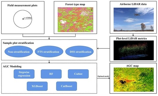
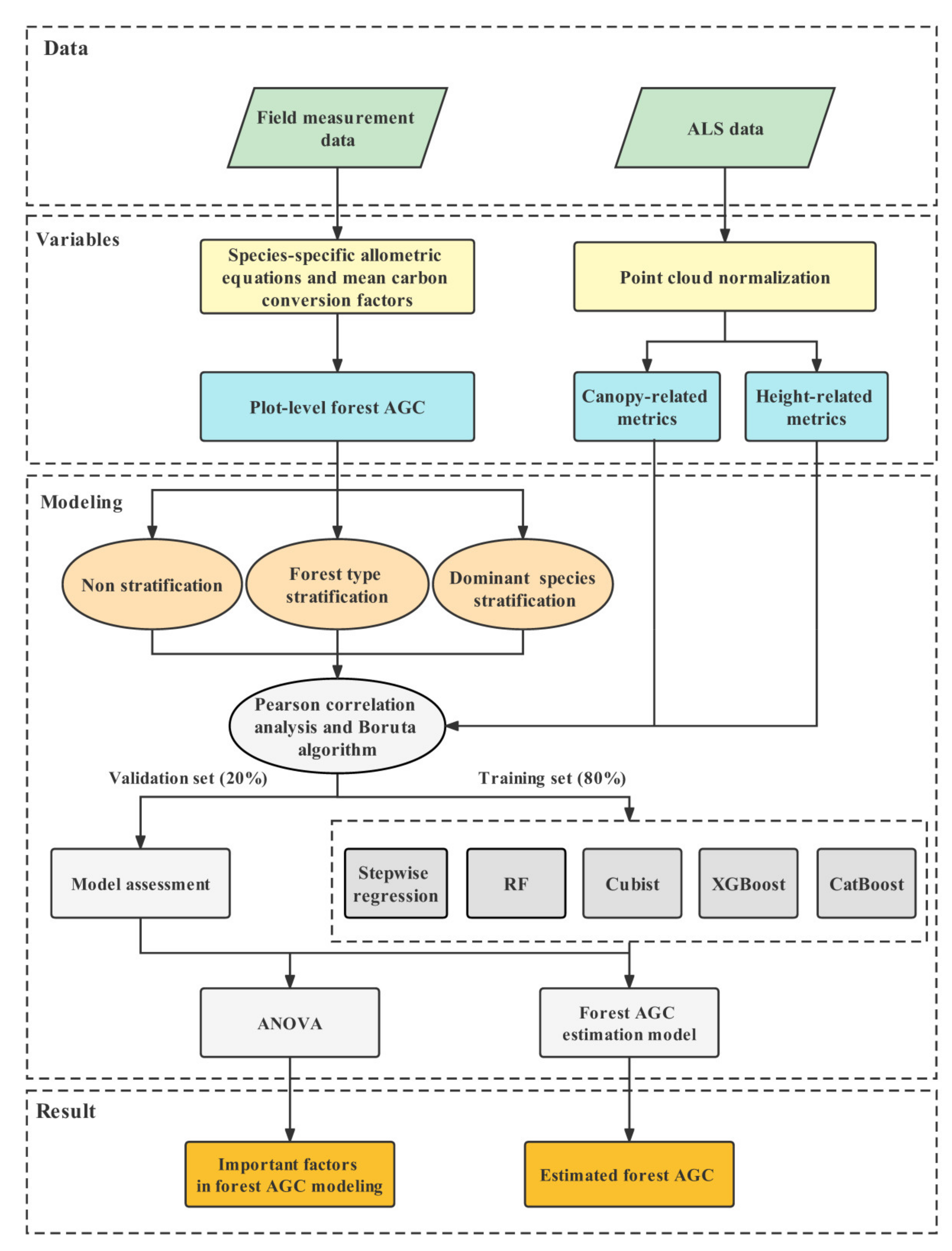
2. Materials and Methods

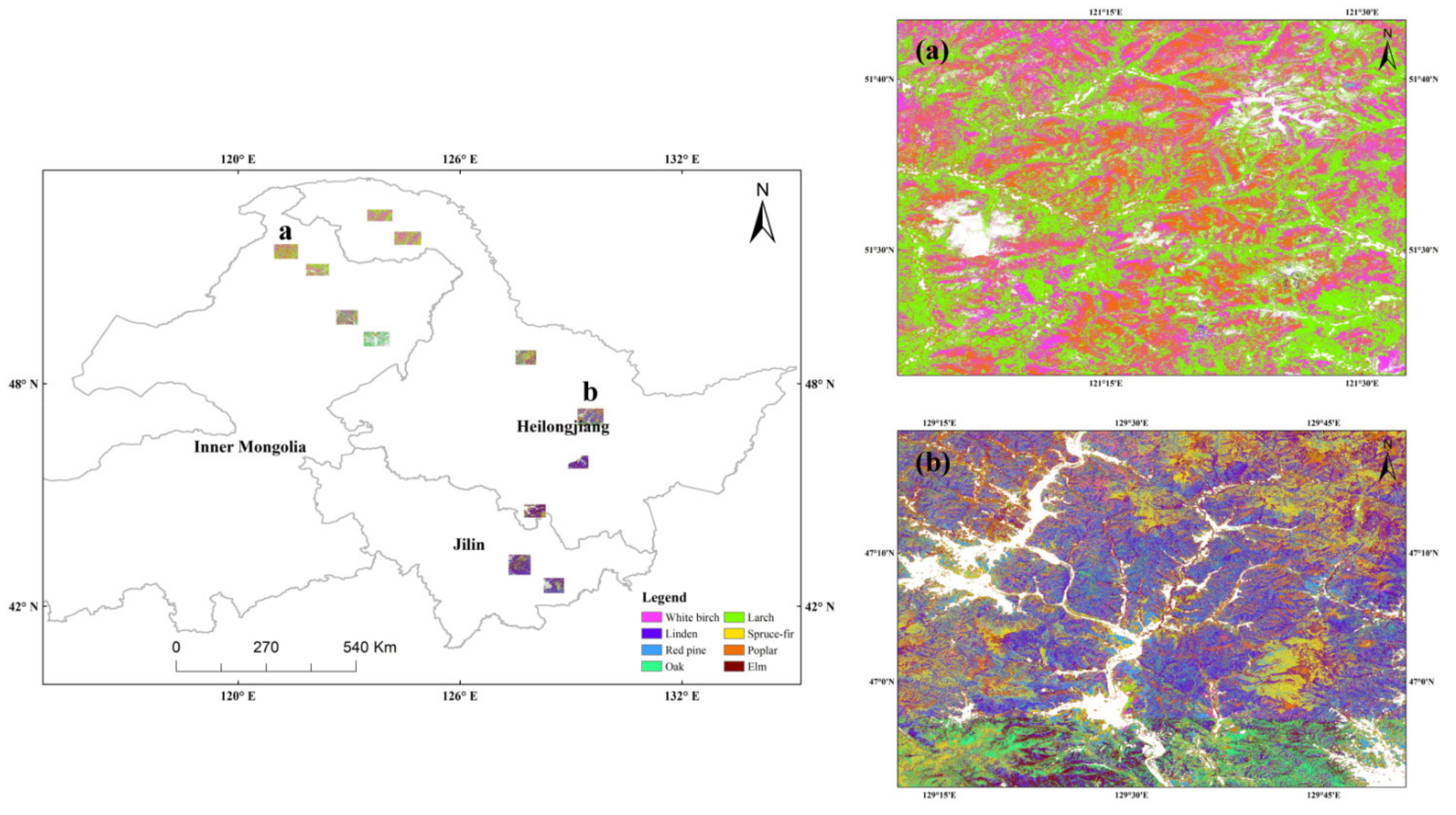
2.1. Study Area

We conducted this study in the forest regions of Northeast China, across three provinces, Heilongjiang, Jilin and Inner Mongolia. The study area covered 12 areas in six forest regions (Figure 1), including the Daxinganling in Inner Mongolia, the Daxinganling in Heilongjiang, the Yichun, the Songhua River, the Mudanjiang and the Changbai Mountain (longitude 119°36′—134°05′E, latitude 41°37′—53°33′N). The climate in most of the region is temperate monsoon, with a cold monsoon climate in the north. The average annual precipitation ranges from 400 to 1000 mm, and the average annual temperature varies between −2 and 2.6 °C. The northeast forest region is surrounded by mountains to the east, north and west, with an average altitude distribution of 500–2500 m. The northeast forest region is one of the richest forest areas in China, with a total forest area of about 680,000 km² and a total forest volume stock of about 3.2 billion m³, accounting for 37% of the country’s total forest area and 30% of the country’s total forest volume stock, respectively (Pan et al., 2011). The Northeast Forest Region contains three zonal vegetation types: cold-temperate coniferous forests, temperate mixed-coniferous forests and warm-temperate deciduous broadleaf forests. The main coniferous species include Larch (Larix gmelinii), Camphor Pine (Pinus sylvestris var. mongolica), Red Pine (Pinus koraiensis) and Spruce (Picea asperata); the main broadleaf species are Poplar (Populus davidiana), White Birch (Betula platyphylla), Oak (Quercus mongolica) and Elm (Ulmus pumila).

2.2. Data Source and Preprocessing

2.2.1. Field Measurements Data and Forest AGC Calculation

The field survey was conducted from September 2019 to November 2019. The dominant species, origin, age group and depression of each stand and the diameter at breast height (DBH), tree height, age and canopy cover of the individual tree that DBH ≥ 6 cm within each plot were measured and recorded by using traditional measuring instruments in the forest inventory. Based on the latest national forest resources inventory results, the distribution of dominant tree species, traffic conditions and other factors in the northeast region, 12 areas covering the target species were typically selected as aerial flight areas for obtaining LiDAR data. A total of 1600 sample plots were randomly collected in these areas, covering five typical forest areas, namely Da Hinggan Ling, Xiao Hinggan Ling, Wanda Mountain, Zhangguangcai Mountain and Changbai Mountain. The sample plots were circular, with a radius of 13.82 m and an area of about 600 m². The quality of the sample plot survey was checked to ensure that the error in DBH measurement was less than 3% and the error in tree height measurement was less than 5%. To ensure the geographic match between the field data and the LiDAR data, clear markers were set up at the center of each sample plot, and Real-Time Kinematic (RTK) technology was used to accurately locate the center of the sample plot, ensuring that the horizontal and vertical coordinates of the sample plot were positioned to within 1 m.

The individual tree data obtained from the field survey were statistically summarized, and the outliers were removed according to the criterion of triple standard deviation; and the data of dead trees were removed to calculate the mean area at breast height, mean diameter at breast height, mean tree height and stand density of the sample plots. After screening, a total of 1587 plots were selected. The AGB was calculated by applying species-specific allometric equations, and then the aboveground carbon stock was received by multiplying by the species-specific mean carbon conversion factor. The allometric equations and carbon-conversion factors for each tree species are shown in

Table 1. Allometric equations and mean carbon conversion factors used in this study.

Tree Species	Allometric Equation	Mean Carbon Conversion Factors
Picea asperata	AGB = 0.08070 × D2.25957 × H0.25663	0.4804
Abies fabri	AGB = 0.06945 × D2.05753 × H0.50839	0.4805
Larix gmelinii	AGB = 0.06848 × D2.01549 × H0.59146	0.4742 (Natural forest) 0.4674 (Plantation)
Pinus koraiensis	AGB = 0.027847 × D1.810004 × H0.905002	0.4809
Populus davidiana	AGB = 0.02884 × D2.8785	0.4956 (Natural forest) 0.4761 (Plantation)
Ulmus pumila	AGB = 0.0607 × D2.4316 + 0.0678 × D1.9623 + 0.0148 × D1.9816	0.4648
Betula platyphylla	AGB = 0.06807 × D2.10850 × H0.52019	0.4656
Quercus mongolica	AGB = 0.06149 × D2.14380 × H0.58390	0.4802
Tilia tuan	AGB = 0.01275 × D2.0188 × H1.0094 + 0.00182 × D1.9492 × H0.9746 + 0.00024 × D1.9814 × H0.9907	0.4677

, with reference to [44,45]. Finally, the individual tree aboveground carbon stock in each plot was summed up and converted into hectares to obtain the forest AGC at plot level.

2.2.2. Design of Sample Plot Stratification

The stratification of sample plots was based on the species information recorded in the field data. In DSS, the criterion for stratification was that one or several tree species account for more than 70% of the entire sample plot in volume stock. The sample plots were therefore stratified (a) to coniferous forests and broadleaf forests (b) to three dominant coniferous tree species, namely Spruce–Fir, Larch and Red Pine, and five dominant broadleaf tree species, namely of Poplar, Elm, Linden, Oak and White Birch. According to Reference [38], strata with smaller populations may return higher prediction errors, which, in turn, can affect the total prediction error. Therefore, to minimize the impact of strata size on the estimation results, we deliberately kept the sample sizes of the eight dominant species strata on a comparable level (approximately 200 sample plots per strata). The detailed information and summary statistics for the forest AGC of each stratification are provided in

Table 2. Overview and distribution of forest AGC of the forest-type-based stratification sample plots.

Forest Type	Number Of Plot			Forest AGC (Mg/ha)
	Total	Training Plot	Validation Plot	Range	Mean	Standard Deviation
Coniferous forests	591	473	118	1.40–82.30	26.23	13.09
Broadleaf forests	996	795	201	0.52–79.83	26.19	11.98
All forests (non-stratification)	1587	1267	320	0.52–82.30	26.20	12.35

and

Table 3. Overview and distribution of forest AGC of the dominant-species-based stratification sample plots.

Dominant Species	Tree Species Composition	Number of Plot			Forest AGC (Mg/Ha)
		Total	Training Plot	Validation Plot	Range	Mean	Standard Deviation
Picea asperata and Abies fabri	Picea asperata dominant forests or Abies fabri dominant forests with a small mixture of Larix gmelinii	197	158	39	2.29–82.30	30.73	15.35
Larix gmelinii	Pure or Larix gmelinii dominant forests with a small mixture of Betula platyphylla and Populus davidiana	197	158	39	1.40–56.13	25.33	12.11
Pinus koraiensis	Pure or Pinus koraiensis dominant forests with a small mixture of Larix gmelinii	197	158	39	1.44–49.13	22.64	9.96
Populus davidiana	Pure or Populus davidiana dominant forests with a small mixture of Larix gmelinii	209	167	42	0.52–79.83	34.36	17.44
Ulmus pumila	Ulmus pumila dominant forests with a small mixture of Populus davidiana	199	159	40	5.81–48.09	23.12	7.62
Betula platyphylla	Pure or Betula platyphylla dominant forests with a small mixture of Larix gmelinii	203	162	41	1.82–52.63	22.17	9.74
Quercus mongolica	Quercus mongolica dominant forests with a small mixture of Pinus tabuliformis	196	157	39	2.27–65.42	25.86	12.07
Tilia tuan	Tilia tuan dominant forests with a small mixture of Larix gmelinii	200	160	40	5.74–42.26	21.71	7.71

. The distribution of the dominant species in the study area is shown in Figure 2. This map was generated from Sentinel-2A images and RF classifier.

2.2.3. Airborne Laser Scanning Data

In order to minimize the impact of forest condition change and errors caused by the time mismatch between field measurements and LiDAR data, airborne LiDAR data were acquired in twelve regions within the six forest regions in September and October 2019, with a total aerial area of 1043 km². Using RIEGL VUX-1UAV airborne laser scanner (RIEGL, Horn, Austria) mounted on a medium rotorcraft UAV platform (Siwei Spatial Data, Beijing, China), with a maximum pulse emission frequency of 550 kHz, a beam divergence angle of 0.5 mrad, a spot diameter of 50 mm, an average point density of about 4 points/m², an average ground point distance of about 1 m, a measurement accuracy of 10 mm, a flight height of about 100 m and a flight speed of 70–110 km/h.

The raw ALS data were processed in the TerraScan modules running on the Microstation platform (TerraSolid, Ltd., Helsinki, Finland) and the LiDAR 360 software (GreenValley, Beijing, China). The main preprocessing procedures include (a) route leveling; (b) point cloud denoising; (c) point cloud filtering—an improved TIN (triangulated irregular network) densification filtering algorithm [46] was used to classify the raw point clouds into the ground or non-ground points; (d) DEM generation, interpolation of the classified ground points using the TIN algorithm [47] to generate DEM; (e) point cloud data normalization—the absolute elevation of each point was subtracted from the DEM, and the height of the point cloud was normalized to remove the elevation effects of the terrain; (f) point cloud data clipping—the point cloud data corresponding to the sample plot was clipped out according to the coordinates of the sample center and the radius information to facilitate the extraction of LiDAR variables; and (g) LiDAR metrics extraction—the 32 LiDAR metrics were extracted from the normalized point clouds within each sample plot with a threshold of 2 m to exclude shrubs and grasses.

2.3. Methods

In this study, we integrated sample plot stratification and ML algorithms to establish forest AGC estimation models based on airborne LiDAR data in the forest regions of Northeast China. Figure 3 showed the framework of the methods for this study. Field measurement data and ALS data were first under preprocessing to obtain plot-level forest AGC and normalized LiDAR data within plots. To explore the effect of stratification in forest AGC estimation, the initial sample plots were stratified into three groups: non-stratification, FTS and DSS (Section 2.2.2). Thirty height-related metrics and 2 canopy-related metrics were extracted from normalized LiDAR data, and Pearson correlation analysis and Boruta algorithms were used to perform variables selection (Section 2.3.1). Then forest AGC estimation models were built based on Stepwise regression and four ML algorithms (RF, Cubist, XGBoost and CatBoost), and independent validation sample plots were used to evaluate the established models (Section 2.3.2 and Section 2.3.5). The analysis of variance (ANOVA) was applied to identify the important factors in forest AGC modeling (Section 2.3.4). Finally, based on the model validation and ANOVA results, the optimal stratification approach and algorithms, and the important factors in forest AGC estimation were derived.

2.3.1. Model Variables Extraction and Selection

Height-related variables and canopy-related variables derived from LiDAR data are suggested to be useful at plot-level estimation and show a high correlation with forest AGB and AGC [48,49]. The height metrics directly describe the vertical height and geometry character of the trees, the density metrics reflect the return density of the trees, the canopy metrics depict canopy structure and the intensity metrics refer to the energy backscattered from the feature to the LiDAR sensor [50,51]. In this study, we extracted 30 height-related and 2 canopy-related variables based on normalized point cloud data with a threshold of 2 m. The detailed information and description of LiDAR metrics are shown in

Table 4. Summary of the metrics extracted from ALS data used in this study.

LiDAR Metrics	Description
CC	Canopy cover
Canopy_relief_ratio	Canopy relief ratio
H_1, H_5, H_10, H_20, H_30,…H_80, H_90, H_95, H_99	Height percentiles. Vertical distribution of point cloud height: 1%, 5%, 10%, 20%, 30%, …, 80%, 90%, 95%, 99% quantile
H_max	Maximum height
H_min	Minimum height
H_mean	Mean height
H_median	Median of height
H_madmedian	Median of median absolute deviation of height
H_sqrt_mean_sq	Generalized means for the 2nd power of height
H_curt_mean_cube	Generalized means for the 3rd power of height
H_AIH_IQ	Interquartile distance of cumulative height
H_IQ	Interquartile distance of height
H_skewness	Skewness of height
H_kurtosis	Kurtosis of height
H_aad	Average absolute deviation of height
H_cv	Coefficient of variation of height
H_stddev	Standard deviation of height
H_variance	Variance of height

.

Although forest AGC is influenced by various factors, not all variables are useful in forest AGC modeling, due to the information redundancy issue. Identifying optimal variables is challenging but the key to establishing a forest AGC estimation model. In this study, Pearson correlation analysis and the Boruta algorithm were used to perform variable selection. The Pearson correlation analysis was first used to select the LiDAR metrics that most correlated with forest AGC. Then, the Boruta algorithm was used to further identify the optimal variables. The core idea of the Boruta algorithm is to construct a shadow feature by randomly mixing the original object feature values to determine whether the importance result of any given feature is significant or not, and then to classify all feature objects in a random forest classification using an extended aggregate with random samples. The maximum Z score among shadow attributes (MZSA) was found and then a two-sided test was performed for each feature object with unassigned importance. Features significantly below the MZSA were considered “unimportant” and features significantly above the MZSA were considered “important”. This process was repeated until all attributes were assigned importance values, resulting in the optimal set of feature variables [52]. All of these procedures were performed in R 4.1.0 using the Boruta packages [52].

2.3.2. Modeling Algorithms

Stepwise regression and four machine-learning algorithms, namely RF, Cubist, XGBoost and CatBoost, were used for forest AGC modeling in this study. Stepwise regression is a parametric algorithm to screen variables and establish the optimal regression equation. In the modeling process of stepwise regression, the predictive variables are input into the regression equation one by one according to the given statistical standard. At each step of the analysis, the predictive variables with the highest correlation with the dependent variables first enter the regression equation, and then the variables are introduced into the model one by one, and the F-test is carried out to judge whether the variable can be selected. Stepwise regression has been widely applied in forest AGB and AGC estimation, as it can remove the variables causing multicollinearity [53,54,55].

RF is an improved machine learning integration algorithm based on decision trees; it was first proposed by Breiman et al. in 2001. Its advantages over traditional decision tree algorithms are that it is insensitive to noisy data, can deal with discrete or continuous data sets and can handle huge datasets [21]. The basic principle of RF is that multiple decision trees are integrated into a single but powerful model, using the “bagging” idea [56], and the Bootstrap resampling technique is used to generate a new training sample set from N original training samples by repeatedly selecting a random k (k < N) sample set. In the whole sampling process, some samples may be taken more than once, while some of the training data will not be sampled. This part of the training data is called “out-of-bag” (OOB) data; the OOB data are not involved in the model-fitting process, but are used to examine the generalization of the model. As randomness can effectively reduce model variance, the RF algorithm can achieve good generalization and low variance resistance without additional “pruning” of the decision trees [57].

Cubist is a rule-based decision-tree model extending from the earlier M5 model, based on which a regression tree is constructed, and generating a linear regression model at the end nodes of the tree, with predictions based on linear regression results at the end nodes rather than on discrete values. The final model of Cubist is a set of multivariate models associated with a set of rules associated with it, where each rule corresponds to a multivariate linear expression. Cubist also uses a boosting-like scheme known as committees, which uses the results of the training set to adjust and create subsequent trees, and then averages the predictions of all committees to generate the final predictions [26]. In addition, the predictions generated by the model rules can be adjusted by using the neighborhoods defined by the parameter neighbors in the training-set data, as this enables Cubist to predict outside of the sample coverage [58].

XGBoost is an ensemble learning algorithm based on the Gradient Boosting Decision Tree (GBDT) framework proposed by Chen and Guestrin in 2016 [59] that has won numerous awards in Kaggle machine-learning competitions and has received widespread attention in recent years. The algorithm is based on the idea of “Boosting” to generate a number of decision trees in turn, combining all the predictions of a set of weak learners to develop a strong learner through an additive training strategy. In contrast to the general GBDT algorithm, the XGBoost algorithm performs a second-order Taylor expansion on the objective function, using the second-order derivatives to accelerate the convergence of the model during training. At the same time, a regularization term is added to the objective function to control the complexity of the tree in order to obtain a simpler model and avoid overfitting [60]. Thus, XGBoost is a flexible and highly scalable tree-structured boosting algorithm with the advantages of being able to handle sparse data, greatly increase the speed of the algorithm, and reduce computational memory in training on very large scale datasets.

CatBoost is a novel gradient boosting decision-tree algorithm developed by Dorogush et al. [61] that belongs to the same boosting family as XGBoost, both being an improved implementation in the framework of the GBDT algorithm. CatBoost uses oblivious trees as base predictors, with fewer parameters and high accuracy, which can also handle categorical features well. In addition, CatBoost has solved the statistical problems of Gradient Bias and Prediction shift that all existing gradient boosting algorithms face by proposing a new and improved gradient boosting algorithm, order boosting, to reduce the occurrence of overfitting and thus improve the algorithm’s accuracy and generalization. The basic idea is, firstly, the CatBoost model correlates the category features to account for the different bases of category features, including calculating the frequency of category occurrences and considering different combinations of category features to construct the regression tree. Secondly, to solve the prediction drift problem caused by gradient bias, random permutations are generated in the training dataset, and gradients are obtained based on it. For training distinct models, different permutations are used; thus, overfitting will not happen. Compared with existing GBDT algorithms, the advantages of CatBoost are the following: (a) using an innovative algorithm that automatically treats categorical features as numerical features, (b) combining category features and making full use of the connections between features greatly enriches the feature dimension and (c) the use of a fully symmetric tree model reduces overfitting and improves the accuracy and generalization of the algorithm [57,62].

Forest AGC estimation is largely dependent on the relationship between tree height and AGC due to the allometric relationships of the tree. Complex forest structure can affect the relationship between forest AGC and tree height and thus interfere with the estimation results. In theory, separate modeling of forest AGC for different dominant species can mitigate this interference and improve the algorithm’s estimation performance. Therefore, in this study, we assume that the finer the stratification and the simpler the forest structure, the better the algorithm’s estimation performance will be. Moreover, the estimation performance of different algorithms may be various due to the differences in forest structure among species. To verify these hypothesizes, three different scenarios were designed: (1) forest AGC models were established based on five algorithms without stratification, resulting in a total of 5 models; (2) forest AGC models were established based on FTS with five algorithms, resulting in a total of 10 models; and (3) forest AGC models were established based on DSS with five algorithms, resulting in a total of 40 models.

2.3.3. Hyperparameter Optimization in Machine Learning Algorithm

Four machine learning algorithms, RF, Cubist, XGBoost and CatBoost, were used in this study. In a machine-learning algorithm, the predicted results and model performance are largely determined by the hyperparameters of the model. A set of hyperparameters should be tuned for each algorithm to obtain the best model performance. The hyperparameters of different machine learning vary greatly, and it is difficult to adjust the parameters manually. Therefore, grid search technology was used to perform hyperparameter tuning automatically. Hyperparameter tuning was performed on the RF, Cubist, XGBoost and CatBoost algorithms based on the lowest RMSE of the model obtained by repeating the 10-fold cross-validation method five times on the training dataset, respectively, to ensure the robustness in the modeling process. All of these procedures were performed in R 4.1.3, using the Caret packages. Details about various hyperparameters and their corresponding grid values are presented in

Table 5. Hyperparameter tuning ranges for four machine learning algorithms.

Algorithm	Hyperparameter	Description	Value Ranges
RF	mtry	the number of predictor variables randomly sampled at each split	(1–n) n refers to the number of predictor variables
	ntree	the number of trees	(100–1000) at intervals of 50
Cubist	committees	the number of trees	(1–100) at intervals of 1
	neighbors	controls the rule-based model predictions	(0–9) at intervals of 1
XGBoost	max_depth	the depth of the tree	(1–10) at intervals of 1
	eta	the learning rate	(0.01–0.5) at intervals of 0.01
	gamma	minimum loss reduction of the tree	(0–1) at intervals of 0.1
	colsample_bytree	the number of predictor variables supplied to a tree	(0–1) at intervals of 0.1
	min_child_weight	minimum number of instances	(1–10) at intervals of 1
	subsample	the number of observations supplied to a tree	(0–1) at intervals of 0.1
CatBoost	depth	the depth of the tree	(1–10) at intervals of 1
	learning_rate	the learning rate	(0.01–0.5) at intervals of 0.01
	l2_leaf_reg	coefficient at the L2 regularization term of the cost function	(0–5) at intervals of 0.1
	rsm	the percentage of features to use at each split selection	(0–1) at intervals of 0.1

.

2.3.4. Statistical Analysis

The two-way analysis of variance (ANOVA) was used to quantify the effect of each factor on the estimation error and to identify the key factors in forest AGC estimation. These factors include the stratification method (non-stratification, FTS and DSS), the regression algorithm (stepwise regression, RF, Cubist, XGBoost and CatBoost) and their interactions. To better show how each factor explains the total variance, we calculated the eta-squared (η²), the proportion of the sum of squares of each factor to the total sum of squares. The ANOVA was performed in R 4.1.0.

2.3.5. Model Validation

To compare the estimation performance of stepwise regression and four machine-learning algorithms in this study, coefficient of determination (R², Equation (1)), root mean square error (RMSE, Equation (2)), relative root mean square error (RRMSE, Equation (3)), mean absolute error (MAE, Equation (4)) and Bias (Equation (5)) were employed. The hold-out method was used for calculating the model performance metrics, and the field measurement data of each stratification were randomly split into a training set (80% of the total) and a validation set (the remaining 20%). The training set was used to train and establish the model, while the validation set was not involved in the model establishing process but acted as an independent sample to evaluate the model performance. After hyperparameter optimization, the best models were built based on the training set, and the model performance metrics were calculated based on the validation set. The higher R², lower RMSE, RRMSE, MAE and Bias values imply a higher prediction accuracy and better estimation results:

$${\mathrm{R}}^2=1-\frac{{\sum }_{i=1}^n{\left(y_i-\widehat{ y_i}\right)}^2}{{\sum }_{i=1}^n{\left(y_i-\overline{y}\right)}^2}$$

(1)

$$\mathrm{RMSE}=\sqrt{\frac{{\sum }_{i=1}^n\left(y_i-\widehat{y_i}\right)²}{n}}$$

(2)

$$\mathrm{RRMSE} = \frac{\mathrm{RMSE}}{\overline{y}} \times 100$$

(3)

$$\mathrm{MAE}=\frac{{\sum }_{i=1}^n\left|y_i-\widehat{y_i}\right|}{n}$$

(4)

$$\mathrm{Bias}=\frac{{\sum }_{i=1}^n(\widehat{y_i}-y_i)}{n}$$

(5)

where n is the number of sample plots, $\widehat{ y_i}$ is the predicted forest AGC, $y_i$ is the field measurement forest AGC and $\overline{y}$ is the mean of field measurement forest AGC.

3. Results

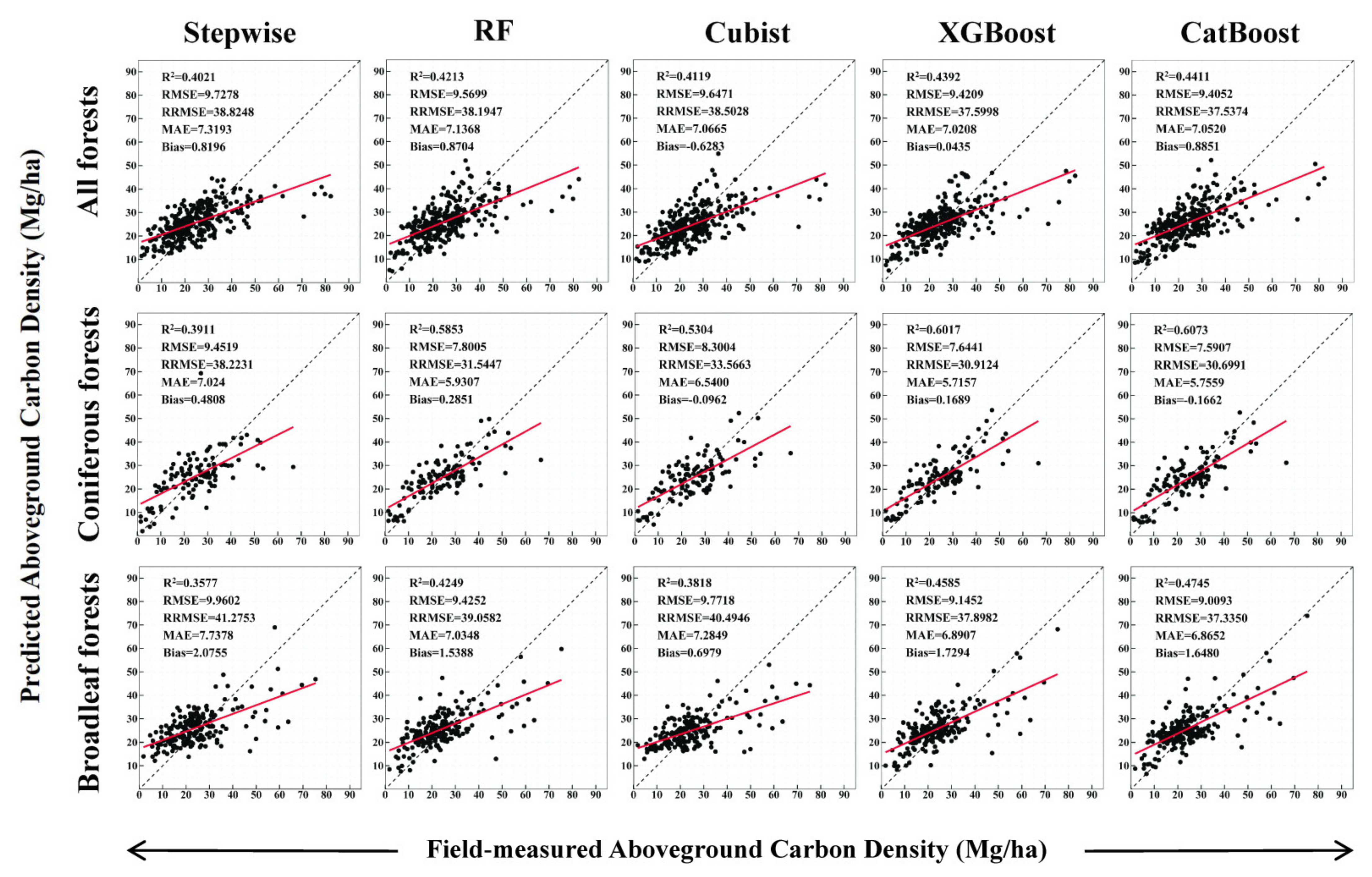
3.1. Comparative Analysis of Forest AGC Estimation Results

3.1.1. Forest AGC Estimation Results Based on FTS

To evaluate the effect of FTS and non-parametric machine-learning algorithms in establishing the forest AGC estimation models, 15 forest AGC estimation models were developed by using stepwise regression and four machine-learning algorithms (RF, Cubist, XGBoost and CatBoost) based on non-stratification and two stratified datasets (coniferous forests and broadleaf forests), respectively. The model performance and evaluation results for the stratified and the unstratified models are shown in

Table 6. Performance of forest AGC estimation model based on non-stratification and FTS in the validation datasets.

Forest Type	Model	R2	RMSE (Mg/ha)	RRMSE (%)	MAE (Mg/ha)	Bias (Mg/ha)
All forests (non-stratification)	Stepwise	0.3948	9.7867	39.0596	7.3902	0.8163
	RF	0.4213	9.5699	38.1947	7.1368	0.8704
	Cubist	0.4119	9.6471	38.5028	7.0665	−0.6283
	XGBoost	0.4392	9.4209	37.5998	7.0208	0.0435
	CatBoost	0.4411	9.4052	37.5374	7.0520	0.8851
Coniferous forests	Stepwise	0.3911	9.4519	38.2231	7.0240	0.4808
	RF	0.5853	7.8005	31.5447	5.9307	0.2851
	Cubist	0.5304	8.3004	33.5663	6.5400	−0.0962
	XGBoost	0.6017	7.6441	30.9124	5.7157	0.1689
	CatBoost	0.6073	7.5907	30.6961	5.7559	−0.1662
Broadleaf forests	Stepwise	0.3577	9.9602	41.2753	7.7378	2.0755
	RF	0.4249	9.4252	39.0582	7.0348	1.5388
	Cubist	0.3818	9.7718	40.4946	7.2849	0.6979
	XGBoost	0.4585	9.1452	37.8982	6.8907	1.7294
	CatBoost	0.4745	9.0093	37.3350	6.8652	1.6480

.

According to the results illustrated in Table 6, the FTS models improved the performance and predicted accuracy when applying machine-learning algorithms, as evidenced by an increase in R² and a decrease in RMSE, RRMSE and MAE, while the reversed results were achieved in stepwise regression models. Compared to the unstratified models, a significant improvement was observed in the coniferous-forest-stratified models, while only a slight improvement in the broadleaf-forest-stratified models, indicating that FTS provided a more positive effect in coniferous forests than broadleaf forests. Overall, four machine learning algorithms outperformed stepwise regression, regardless of the datasets used. The CatBoost models achieved the best estimation performance in all the three datasets, with the highest R² (0.4411 in all forests, 0.6073 in coniferous forests and 0.4745 in broadleaf forests), lowest RMSE (9.4052 in all forests, 7.5907 in coniferous forests and 9.0093 in broadleaf forests), RRMSE (37.5374 in all forests, 30.6961 in coniferous forests and 37.3350 in broadleaf forests) and MAE (6.8652 in broadleaf forests), followed by XGBoost, RF, Cubist and stepwise regression. The Bias of the CatBoost models in the three datasets were 0.8851, −0.1662 and 1.6480 Mg/ha, respectively, suggesting a general overestimation of forest AGC in unstratified and broadleaf forest models, as well as a general underestimation of forest AGC in coniferous forest models.

The improvement provided by the FTS models can be further evidenced in the scatter plots between the field-measurement forest AGC and model estimated values (Figure 4). Figure 4 shows the correlation between the estimated forest AGC and the reference data based on FTS is better compared to the non-stratification ones except the models using stepwise regression. Moreover, a significant underestimation is observed when the forest AGC is larger than 40 Mg/ha in all the 15 models, while a significant overestimation is observed when the forest AGC is lower than 10 Mg/ha in unstratified and broadleaf forests models. However, the extent of overestimation and underestimation is reduced when using FTS.

3.1.2. Aboveground Carbon Density Estimation Results Based on DSS

To examine the influence of DSS and ML algorithms in the forest AGC estimation, we compared and analyzed the model validation results of the forest AGC models established by using stepwise regression and four machine-learning algorithms (RF, Cubist, XGBoost and CatBoost) based on eight DSS datasets (Spruce-Fir, Larch, Red Pine, Poplar, White Birch, Oak, Linden and Elm), respectively, resulting in a total of 40 models. The results of model performances are summarized in

Table 7. Performance of forest AGC estimation models based on DSS in the validation datasets.

Dominant Species	Model	R2	RMSE (Mg/ha)	RRMSE (%)	MAE (Mg/ha)	Bias (Mg/ha)
Spruce–Fir	Stepwise	0.7371	6.8977	23.4290	5.3067	−0.1559
	RF	0.7547	6.6623	22.6294	4.9116	0.1994
	Cubist	0.7493	6.7361	22.8801	5.2763	0.4992
	XGBoost	0.7936	6.1119	20.7600	4.5688	−0.3968
	CatBoost	0.8175	5.7463	19.5181	4.2701	1.0252
Larch	Stepwise	0.6931	6.5371	28.4119	4.9649	1.7802
	RF	0.6273	7.2045	31.3124	5.8318	1.9752
	Cubist	0.6854	6.6184	28.7652	5.2080	0.5859
	XGBoost	0.7047	6.4125	27.8701	4.8272	1.1372
	CatBoost	0.7304	6.1274	26.6309	4.7103	1.1988
Red Pine	Stepwise	0.7864	4.8843	21.8278	3.6780	−1.0045
	RF	0.8351	4.2915	19.1786	3.2918	−0.7201
	Cubist	0.8014	4.7098	21.0482	3.8554	−1.0005
	XGBoost	0.8509	4.0810	18.2380	3.3971	−0.1736
	CatBoost	0.8699	3.8113	17.0328	3.2853	0.1476
Poplar	Stepwise	0.6751	8.9241	23.6450	6.8659	−0.9275
	RF	0.7607	7.6595	20.2943	6.0103	−0.0022
	Cubist	0.7486	7.8506	20.8007	6.1131	0.5429
	XGBoost	0.7778	7.3812	19.5569	5.8989	0.1414
	CatBoost	0.8054	6.9076	18.3022	5.2377	−0.0178
White Birch	Stepwise	0.7211	5.3155	24.7447	4.1372	0.2416
	RF	0.7407	5.0642	23.5747	3.7654	0.2466
	Cubist	0.7662	4.8671	22.6570	3.5408	−0.2407
	XGBoost	0.7636	4.8943	22.7840	3.5005	0.0718
	CatBoost	0.7852	4.6653	21.7180	3.6770	−0.1229
Oak	Stepwise	0.6362	6.6328	27.7826	4.8668	0.9758
	RF	0.7468	5.5342	23.1808	4.0921	0.1669
	Cubist	0.7386	5.6229	23.5524	3.9071	0.1812
	XGBoost	0.7652	5.3294	22.3229	4.0862	−0.5591
	CatBoost	0.7903	5.0355	21.0920	3.8465	0.3638
Linden	Stepwise	0.3224	6.5837	30.2533	5.0754	0.7719
	RF	0.5294	5.4869	25.2136	4.1952	0.4577
	Cubist	0.4821	5.7557	26.4485	4.2222	0.3208
	XGBoost	0.5450	5.3949	24.7906	4.1490	0.2983
	CatBoost	0.6327	4.8474	22.2750	3.8665	0.5140
Elm	Stepwise	0.5362	4.8298	20.4512	3.9670	0.9204
	RF	0.5959	4.5080	19.0887	3.7378	1.2237
	Cubist	0.5448	4.7845	20.2596	3.9858	1.1691
	XGBoost	0.6308	4.3089	18.2456	3.5939	0.9103
	CatBoost	0.6906	3.9446	16.7032	3.1906	0.5471

and Figure 5.

Figure 5 illustrates the estimation accuracy of forest AGC varies with different dominant species. In terms of algorithm performance, estimation models based on DSS show similar trends to those based on FTS; that is, the four machine-learning algorithms outperform the stepwise regression, with the CatBoost models achieving the highest estimation accuracy, followed by XGBoost, RF, Cubist and stepwise regression. The detailed information of the model evaluation results can be found in Table 7. Table 7 shows the 40 models for eight different dominant species with R² varying from 0.3224 to 0.8699, RMSE varying from 3.8113 to 8.9241, RRMSE varying from 16.7032 to 31.3124, MAE varying from 3.1906 to 6.8659 and Bias varying from −1.0045 to 1.9752. Relatively high estimation accuracy was achieved in all eight dominant species, with the CatBoost model based on DSS for Red Pine achieving the best estimation accuracy (R² = 0.8699, RMSE = 3.8133, RRMSE = 17.0328, MAE = 3.2853 and Bias = 0.1476). In terms of Bias, no single algorithm is optimal in all dominant species, with the highest mean Bias (1.2755) being observed in the Larch models, indicating a more significant overestimation of forest AGC in the Larch, regardless of the algorithm used. Overall, the models established based on DSS achieved much higher estimation accuracy compared to the unstratified models (Table 6), and this improvement is more significant in the Spruce–Fir, Larch, Red Pine, Poplar, White Birch and Oak models. The estimated forest AGC of eight dominant species models based on the CatBoost algorithm was shown in Figure 6. The mean estimated forest AGC ranged from 21.36 to 37.72 Mg/ha in eight dominant species, with the estimated forest AGC of Poplar and Spruce–Fir being significantly higher than the other dominant species, and the estimated forest AGC of the remaining dominant species were at a comparable level.

The scatter plots between the field-measurement forest AGC and estimated values for the eight dominant species are provided in Figure 7. Figure 7 shows that the linear relationships between the estimated and measured values of forest AGC are relatively better in Spruce–Fir, Larch, Red Pine, Poplar, White Birch and Oak models, while relatively poor linear relationships are observed in Linden and Elm. A significant underestimation is observed when the forest AGC is larger than 40 Mg/ha in Larch, Poplar and Oak models, while a significant overestimation is observed when the forest AGC is lower than 20 Mg/ha in Larch, Poplar, Linden and Elm models. Compared to the unstratified models (Figure 4), the linear relationships between the estimated and measured values of forest AGC and the extent of overestimation and underestimation are greatly improved in all 40 models established based on DSS. The forest AGC estimation models based on DSS have achieved much better estimation performance than unstratified ones.

3.1.3. Comparative Analysis of Forest AGC Estimation Results Based on FTS and DSS

To further explore the optimal stratification method in forest AGC estimation, the overall estimation accuracy of models based on non-stratification, FTS and DSS were summarized in

Table 8. Summary of the overall estimation accuracy of non-stratification, FTS and DSS models on the validation datasets.

Stratification Method	Model	R2	RMSE (Mg/ha)	RRMSE (%)	MAE (Mg/ha)	Bias (Mg/ha)
Non-stratification	Stepwise regression	0.3948	9.7867	39.0596	7.3902	0.8163
	RF	0.4213	9.5699	38.1947	7.1368	0.8704
	Cubist	0.4119	9.6471	38.5028	7.0665	−0.6283
	XGBoost	0.4392	9.4209	37.5998	7.0208	0.0435
	CatBoost	0.4411	9.4052	37.5374	7.0520	0.8851
FTS	Stepwise regression	0.3700	9.7752	40.1415	7.4738	1.4856
	RF	0.4826	8.8590	36.3788	6.6264	1.0751
	Cubist	0.4353	9.2548	38.0042	7.0094	0.4042
	XGBoost	0.5101	8.6205	35.3995	6.4561	1.1522
	CatBoost	0.5223	8.5121	34.9546	6.4549	0.9769
DSS	Stepwise regression	0.7309	6.4663	25.3713	4.8700	0.3162
	RF	0.7737	5.9307	23.2698	4.5070	0.4091
	Cubist	0.7705	5.9719	23.4313	4.5200	0.2599
	XGBoost	0.7984	5.5975	21.9624	4.2611	0.1803
	CatBoost	0.8232	5.2421	20.5680	4.0169	0.4493

. Generally, the CatBoost models based on DSS have achieved the best estimation accuracy (R² = 0.8232, RMSE = 5.2421, RRMSE = 20.5680, MAE = 4.0169 and Bias = 0.4493), while the stepwise regression models based on FTS provided the worst estimation accuracy (R² = 0.3700, RMSE = 9.7752, RRMSE = 40.1415, MAE = 7.4738 and Bias = 1.4856). The comparative results illustrate that the estimation accuracy of models based on DSS is significantly higher than that of models based on FTS, regardless of the algorithm used, with R² increased from 0.3700~0.5223 to 0.7309~0.8232, RMSE reduced from 8.5121~9.7752 to 5.2421~6.4663, RRMSE reduced from 34.9546~40.1415 to 20.5680~25.3713, MAE reduced from 6.4549~7.4738 to 4.0169~4.8700 and Bias reduced from 0.4042~1.4856 to 0.1803~0.4493. As the CatBoost models based on DSS have provided the highest estimation accuracy, they were chosen for mapping the spatial distribution of the estimated forest AGC in the study area (Figure 8). Moreover, compared to the non-stratification models, a significant improvement was observed in DSS models, while only a slight improvement was observed in FTS models.

Further comparison of scatter plots of field-measured forest AGC and estimated values between FTS models (Figure 4) and DSS models (Figure 6) illustrates that the linear relationships between the estimated and measured values of forest AGC and the extent of overestimation and underestimation are greatly improved in all 40 models established based on DSS. In summary, the forest AGC estimation model established by each dominant species has a higher predictive ability and applied potential than the models constructed by each forest type.

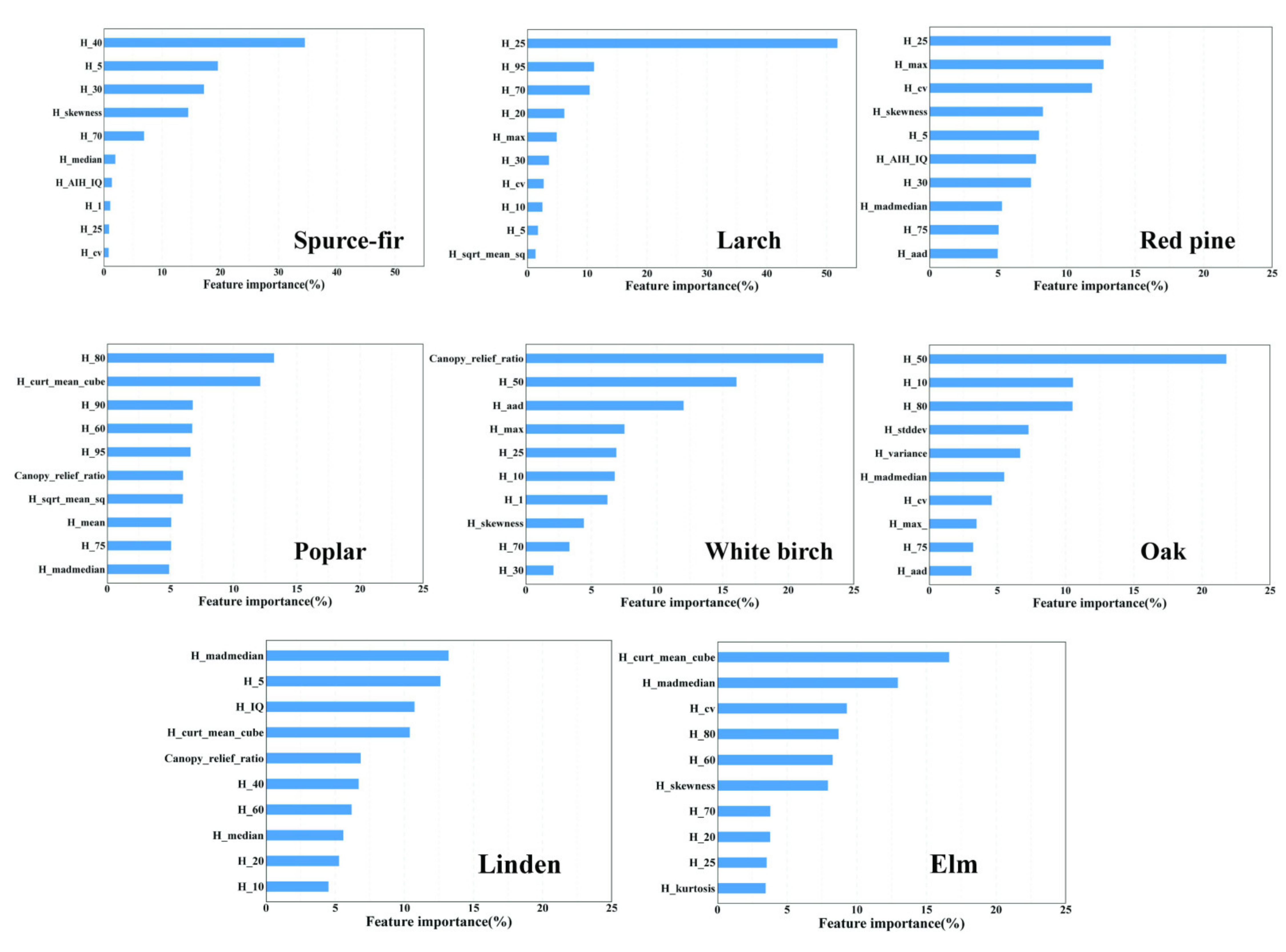
3.2. Variable Importance Analysis

The variable importance for forest AGC estimation models was evaluated by the PredictionValuesChange method based on CatBoost in the DSS models. The relative importance of the 10 highest ranked variables was shown in Figure 9, revealing that the important variables vary in different dominant species models. The height percentile metrics have achieved the highest relative importance in most of the DSS models, accounting for more than 80% in the Larch model, more than 70% in the Spruce–Fir model, more than 40% in the Oak model, more than 30% in the Red Pine, Poplar, White Birch and Linden model and more than 25% in the Elm model. Canopy-related metrics are also useful in the forest AGC estimation, with the canopy relief ratio metric being the most important variable in the White Birch models and the fifth and sixth important variable in Linden and Poplar model. In general, the height-related metrics and canopy-related metrics play an important role in forest AGC estimation, with height-related metrics being more important. The variables importance analysis results demonstrate that the important variables for the models vary with dominant species, illustrating the necessity to identify optimal model variables for forest AGC estimation models in different dominant species.

4. Discussion

4.1. Variables Selection in Forest AGC Estimation

Identifying suitable variables is a prerequisite and key to building a high-precision forest AGC estimation model. The commonly used variables derived from LiDAR data in forest AGB and AGC estimation can be divided into four categories: height, density, intensity and canopy metrics [63,64,65]. In this study, the initial LiDAR dataset contained 30 height-related and two canopy-related variables, without considering density and intensity variables. It is based on the prior knowledge that density and intensity metrics are often influenced by many other factors, including transmitted power, range, angle of incidence, atmospheric transmittance, environmental parameters and the structural characteristics of the target itself [66], resulting in the density and intensity values obtained for the same feature on different flight routes varying significantly and making it difficult to reflect the true character of the feature. Moreover, several studies have proposed that LiDAR intensity values must be calibrated before they can be applied to forest AGB and AGC estimation [67,68], but to date, no standard approach for LiDAR intensity correction has been established. Then Pearson correction analysis and the Boruta algorithm were used to further provide auxiliary information on variable selection for each dataset. Feature selection based on expert knowledge allows for the selection of the most useful variables in AGC estimation from an empirical perspective, while correlation analysis and automated feature selection algorithms provide the best set of variables from a statistical perspective. It was also suggested in Reference [11] that the inclusion of expert knowledge in variables selection would make the model more ecologically meaningful and generalized than those using only automatic feature-selection algorithms, such as stepwise regression, RFE and Boruta.

The variable importance analysis results showed that the height percentile metrics are the most important in most cases, which is consistent with several previous studies [20,58], revealing the high corrective between height percentile metrics and forest AGC. In addition, the variable importance results also demonstrated that the important variables are different in different dominant species. Thus, there are possibly two ways to improve the large-scale forest AGC estimation: One is to select optimal variables for a specific study area. In this case, considering the experience and previous effort on AGC estimation in variables selection of the specific study region may be more effective before modeling. The other is to examine the potential generic indicators that are independent of geographical and environmental conditions, e.g., the TCH metric derived from ALS data [69] and LiDAR biomass index (LBI) obtained from TLS data [70]. However, the extent to which these indicators are effective remains to be tested, and more studies should be carried out on the model transferability to provide accurate forest AGC estimation on a large scale.

4.2. The Role of Stratification in Forest AGC Estimation

Our study indicated that both FTS and DSS could improve the estimation accuracy of forest AGC compared to non-stratification estimation, which confirmed the effectiveness of stratification in forest AGC estimation and was consistent with previous studies [71,72]. The essence of stratified estimation is to aggregate observations of target variables into more homogeneous strata or levels than the whole. Forest AGC varies greatly across different forest types and dominant species, as forest AGC is related to a variety of factors, such as forest structure, species composition, stand characteristics and site factors. The heterogeneity between different forests makes the relationship between forest AGC and tree height becoming particularly complex and limit the estimation accuracy of LiDAR data. Stratifying the sample plots into forest types or dominant species can reduce forest heterogeneity arisen from the interference of other factors in AGC estimates, thus improving the correlation between forest AGC and LiDAR metrics. Moreover, allometric models and carbon conversion factors are developed at the tree species level, and thus the AGC estimation models should be established on individual forest type or dominant species to reduce the uncertainty [16].

A two-way ANOVA was used to explore the important factors in forest AGC estimation. The ANOVA results (

Table 9. ANOVA of the R², RMSE, RRMSE and MAE respective to the stratification method, regression method and their interaction.

Factor	Df	R2 SumSq	η2	RMSE SumSq	η2	RRMSE SumSq	η2	MAE SumSq	η2
Stratification	2	0.65	0.53	123.45	0.66	2171.4	0.77	63.89	0.64
Regression method	4	0.10	0.08	8.39	0.05	131.1	0.05	4.51	0.05
Stratification: regression method	8	0.01	0.01	0.68	0.00	11.5	0.00	0.50	0.01
Residuals	40	0.47		53.52		511.3		30.57

) showed that the stratification method had the most significant effect on the estimation error, explaining 53% of the total variance in R², 66% of the RMSE, 77% of the RRMSE and 64% of the MAE. The regression algorithm and its corresponding interactions had a marginal impact on estimation accuracy, explaining less than 10% of the total variance in R², RMSE, RRMSE and MAE, respectively. The ANOVA results proved that a stratification of the sample plots is of greater importance than the modeling algorithm, which was inconsistent with Reference [38]. The discrepancy may be contributed to the differences in stratification method, sample size and the study area; thus, more studies should be conducted to further examine the generalizability of our results.

4.3. FTS versus DSS

The comparative results between FTS and unstratified estimates show that significant improvement was obtained in AGC estimation models based on coniferous forest, while only marginal improvement was obtained in AGC estimation models based on broadleaf forest. One possible explanation for this is to be found in the substantial differences in tree crowns and distribution of branches and leaves across different broadleaf tree species in this study, which heavily affects the penetration of the laser pulses and thus influences the relationships between LiDAR metrics and forest AGC [73]. It is also mentioned by Reference [21] that AGB modeling based on coniferous forest provided poorer estimation performance due to the difference in crown size, shape and the relationship between the AGB and canopy height of the Masson pine and Chinese fir. Therefore, stratifying the sample plots into the coniferous forest and broadleaf forest may not be sufficient to reduce the heterogeneity within strata and provide better estimation performance. In addition, a higher estimation accuracy was obtained in the coniferous forest than in the broadleaf forest, as is consistent with several previous studies [74,75]. The difference may be attributed to the fact that broadleaf tree species tend to have more biomass in the branches and weaken the relationships between height and forest AGC [76].

Further comparison of the estimation performance between the FTS and DSS models illustrated that a substantially higher R², RMSE, RRMSE, MAE and Bias were observed in DSS models, and this is in line with previous studies [21,77]. The results demonstrate that DSS is a more recommended approach for stratification estimation. The improvement provided by DSS can be attributed to the fact that the relationships between tree height and forest AGC are the same in individual tree species, as they share similar canopy structures and AGB distribution. Stratifying sample plots into dominant species can provide highly homogenous strata and minimize the within-strata variance, leading to a better forest AGC estimation. However, there are also several studies reporting that only minor improvements in estimation performance were obtained when the same data were used to construct individual forest type or species strata for estimation [38,78,79]. The difference in results may be attributed to inconsistent sample sizes across different studies and small sample sizes within strata in most studies. Higher uncertainty and prediction errors may be produced with fewer within-strata sample sizes, and these, in turn, affect the total prediction error. For example, the Douglas fir and maple had the highest RMSD value for 261% and 315%, which accounted for the smallest number of overall sample plots (7.0% and 5.7%) [80]; the subtropical Picea abies forest (SPAF) had the highest RMSE (82.7 ± 28.2 Mg/ha) and bias (−36.8 ± 19.5 Mg/ha) with the smallest number of reference data (16) [81]. It is also mentioned by Reference [82] that estimates of standard errors can be biased in the case of small sample sizes within strata. In this study, the within-strata sample plot sizes of each dominant species were kept at around 200, which is a comparable and relatively large level, making the estimation results more robust and representative.

4.4. Machine-Learning Algorithms for Forest AGC Estimation

Modeling algorithms have been suggested to be an important factor for the accurate estimation of forest AGB and AGC [83]. However, to date, no single algorithm has been optimal in all cases. Therefore, identifying a proper algorithm has been a critical step to constructing AGC estimation models. In this study, the estimation performances of one parametric approach (Stepwise regression) and four non-parametric machine learning algorithms (RF, Cubist, XGBoost and CatBoost) were compared. The results showed that four machine-learning algorithms outperform stepwise regression in most cases, thus confirming previous findings that non-parametric machine-learning algorithms were suggested to be more suitable for forest AGB and AGC estimation than the parametric algorithm [22,24,25]. We attribute the better performance of ML algorithms to the fact that the relationships between forest AGC and the LiDAR metrics are likely nonlinear and complex, especially in those forests with complex stand structures and tree species composition, and this makes it difficult to model these relationships through parametric algorithms with a fixed model structure. However, overestimation of forest AGC at low AGC values and underestimation of forest AGC at high values are still common in ML algorithms. Moreover, the hyperparameter tuning methods and tuning ranges vary with study area and input data, which greatly limit the model transferability of ML algorithms. Moreover, we found that, when forest AGC estimation models were established based on DSS, a significant improvement was observed in stepwise regression models, implying that the relationships between forest AGC and the LiDAR metrics are expected have a more linear association at the species level.

Among the four ML algorithms, two novel boosting-based ensemble algorithms, XGBoost and CatBoost, have provided better forest AGC estimation accuracy than others, and the CatBoost algorithm outperformed other algorithms in all datasets. Before this study, XGBoost and CatBoost algorithms have not been used for forest AGC estimation, but there have been several studies on forest AGB estimation. Pham et al. [84] combined a genetic algorithm (GA) and XGBoost to achieve the best estimation of mangrove AGB than other four ML algorithms (RF, SVM, GBRT and CatBoost); Zhang et al. [85] compared and evaluated the performance of eight ML algorithms (MARS, RF, SVM, GBRT, ANN, SGB, ERT and CatBoost) in forest AGB estimation, and the results showed that CatBoost provided the best performance with an R² of 0.72, an RMSE of 45.63 Mg/ha, a bias of 0.06 Mg/ha, and a relative RMSE of 25%. Luo et al. [86] examined the different combinations of three feature selection methods and three ML algorithms (RF, XGBoost and CatBoost) in forest AGB estimation and found that combining RFE and CatBoost obtained the highest estimation accuracy. The compared results in this study were consistent with these previous studies and further demonstrated the superiority and application potential of XGBoost and CatBoost in forest AGC estimation. Compared with XGBoost, CatBoost has achieved better estimation with fewer hyperparameters, higher model efficiency and slighter overestimation and underestimation problems, making CatBoost a more recommended algorithm in forest AGC estimation. However, more studies should be carried out to further examine the application potential of CatBoost across various forest types within different geographical environments.

4.5. Species-Level Forest AGC Estimation

In this study, we established eight species-level forest AGC estimation models by using CatBoost algorithms and achieved satisfactory estimation accuracy. Our species-level estimation accuracy (R² = 0.63~0.87) was significantly higher than that of Fu et al. (R² = 0.14~0.56) [42] and Zhang et al. (R² = 0.01~0.47) [87], which linked field measurement plots and MODIS data to map species-level biomass in Northeast China. High estimation accuracy has been achieved in Spruce–Fir, Larch, Red Pine, Poplar, White Birch and Oak, while relatively low-estimation accuracies were achieved for Linden and Elm. The discrepancy may be explained by allometric equations and mean carbon conversion factors used for Linden and Elm. The sample plots of Linden and Elm spanned six flight regions and Heilongjiang and Jilin two provinces, with a difference of more than 10 degrees in latitude between north and south. However, the allometric equations and mean carbon conversion factors used for Linden and Elm in this study were not established for a specific region but for the whole Northeast China region. The differences in hydrothermal conditions caused by the latitude could have a significant effect on the growth of Linden and Elm, and these difference, in turn, increase the uncertainty and errors of allometric equations and mean carbon-conversion factors. Moreover, the relatively low-point cloud density of the LiDAR data used in this study (4 points/m²) may not be enough to fully capture the structure information, leading to the poorly structured Linden and Elm models. To our knowledge, species-level forest AGC estimation models in northeast forest regions of China based on LiDAR data have not yet been reported in studies. Species-level AGC estimation models can provide important basic information for large-scale forest resource monitoring, but they pose new challenges in terms of sample size and accurate forest classification products. The lack of spectral information from LiDAR sensors makes it difficult to achieve accurate dominant species maps based on LiDAR data. Therefore, using LiDAR as a sampling tool and fusing LiDAR with other sensors (e.g., hyperspectral and optical) to acquire dominant species area and build forest AGC models could be a potential solution [88,89].

4.6. Uncertainty Analysis and Limitations

Identifying and understanding the uncertainty of the remote sensing-based forest AGC estimation models is necessary for improving forest AGC estimation accuracy and establishing standard estimation designs and procedures [90]. In addition to the errors and uncertainties introduced by the variable selection methods, model algorithms themselves, there are a number of external factors that can contribute to uncertainty in this study. (1) The first factor is the allometric equations and mean carbon conversion factors used for estimating plot-level forest AGB and forest AGC. The errors in allometric equations have been regarded as a common and primary source of uncertainty in forest AGB and AGC estimations [91,92,93]. The sample plots in this study were located in three provinces, Heilongjiang, Jilin and Inner Mongolia, while the species-specific allometric equations and mean carbon conversion factors used were developed for the entire Northeast China region. The allometric equations depend on the assumptions of the allometric relationships between diameter at breast height (DBH) and tree height (H), and these allometric relationships may vary with environment and stand structure, resulting in different forest AGB estimations and great uncertainty. The uncertainty propagates and accumulates with the error in the carbon conversion factors, influencing the final estimation accuracy of forest AGC. (2) The second factor is the errors from small trees shrubs and herbs. In this study, the trees smaller than 6 cm in DBH, as well as shrubs and herbs, were not recorded in the ground survey, which could be captured by the LiDAR data. The cumulative AGC of these small trees, shrubs and herbs may become a non-negligible part of the total and thus introduce errors into the forest AGC estimates. (3) The third factor is the effect of point density. The point density used in this study was 4 points/m², which is low-density point cloud data. Previous studies have demonstrated that the ability of LiDAR to estimate vegetation height decreases with lower point density [94,95]. The relative low point density in this study has limited the detection of the vegetation canopy and the number of points that penetrate to the ground, which may affect the DEM generation and the canopy and height-based forest AGC estimation. (4) The fourth factor is the edge effect and geolocation error. The effect of edge effect may be attributed to the fact that the field measurement is based on the position of the stem while the LiDAR data capture the tree crown and height information within the whole specific region. Therefore, some trees detected by LiDAR data may not be recorded by the ground survey, thus contributing to the uncertainty in the forest AGC estimation. The field sample plots are usually located by consumer-grade GPS whose positional accuracy largely depends on the open conditions of the environment, leading to location error from 1 to 10 m in the complex environment of forest [96]. The mismatch of geographic location between LiDAR data and sample plots data may provide great uncertainty and error in forest AGC estimation. (5) The fifth factor is the error from field measurement. In this study, tree metrics, such as DBH and tree height, were measured manually, using traditional tools. It is usually difficult to locate the treetop in forests with high canopy closure and complex structures. Therefore, the quality and accuracy of these metrics are largely determined by the quality and skill level of the surveyors, which may introduce errors and uncertainty into the results. The advent of advanced technologies, such as ground-based LiDAR and backpack LiDAR, promises to act as a new alternative to reduce uncertainty and improve the accuracy of ground survey.

Some sources of uncertainty, such as the edge effects and geographical location errors, are difficult to quantify empirically and statistically, as it is impossible to find an ideal sample free of the effects of edge effects and geographical location errors. The advent of simulation studies promises to be a powerful tool to solve the present limitations and better quantify and understand uncertainties in forest AGB and AGC estimations. For example, Knapp et al. [97] quantified the effect of border effects by using the bottom-up simulation method, and the simulation results showed that the edge effects decreased with increasing plot sizes, with the edge effects being most significant at the 10 m scale and having no influence at the 100 m scale. There are also several studies using similar simulation methods to successfully qualify the uncertainty introduced by the geolocation error [98], allometric equations [92] and forest structure [99]. Future studies should consider multiple uncertainties simultaneously and quantify the weight of each component to better understand the uncertainty in the entire process of forest AGC estimation.

5. Conclusions

In this study, we retrieved the potential of integrating sample plots stratification and non-parametric machine-learning algorithms for forest AGC modeling in the forest regions of Northeast China. Four major conclusions can be drawn:

(1)

The ANOVA result showed that the stratification method had a more important effect on forest AGC estimation than the regression algorithm. Both FTS and DSS were effective in improving the estimation accuracy of forest AGC compared to non-stratified models, demonstrating the positive role of stratification in forest AGC estimation. Compared to the non-stratified models, the estimation accuracy of forest AGC was significantly improved in coniferous species, while marginal improvement was observed in the broadleaf species.

(2)

Compared with FTS, models based on DSS achieved greater improvements, indicating that DSS is a better stratification estimation method for forest AGC.

(3)

Regardless of the stratification method used, of the five algorithms, the four non-parametric ML algorithms outperformed parametric stepwise regression, with the CatBoost algorithm obtaining the best estimation performance, followed by XGBoost, RF, Cubist and stepwise regression.

(4)

The most important LiDAR metrics for forest AGC estimation were the height percentiles and the canopy relief ratio.

(5)

The CatBoost models based on DSS achieved the highest estimation accuracy, with R² = 0.8232, RMSE = 5.2421, RRMSE = 20.5680, MAE = 4.0169 and Bias = 0.4493. The estimation values of the best forest AGC estimation model for the eight dominant species ranged from 21.36 to 37.72 Mg/ha, with the Poplar having the highest forest AGC and the White Birch having the lowest.

The main contribution of this study is the successful combination of DSS and the CatBoost algorithm to improve the estimation performance of forest AGC and to obtain the first high-precision species-level forest AGC estimation models based on the CatBoost algorithm in the forest regions of Northeast China. Integrating this strategy with the national forest inventory or accurate remote-sensing-based wall-to-wall dominant species classification products is expected to provide a new solution to reduce the uncertainty and improve the estimation accuracy of large-scale forest carbon stock.

References

1. Pan, Y.; Birdsey, R.A.; Fang, J.; Houghton, R.; Kauppi, P.E.; Kurz, W.A.; Phillips, O.L.; Shvidenko, A.; Lewis, S.L.; Canadell, J.G.; et al. A Large and Persistent Carbon Sink in the World’s Forests. Science 2011, 333, 988–993. [Google Scholar] [CrossRef] [PubMed] [Green Version]
2. Six, J.; Callewaert, P.; Lenders, S.; De Gryze, S.; Morris, S.J.; Gregorich, E.G.; Paul, E.A.; Paustian, K. Measuring and Understanding Carbon Storage in Afforested Soils by Physical Fractionation. Soil Sci. Soc. Am. J. 2007, 66, 1981–1987. [Google Scholar] [CrossRef] [Green Version]
3. Lin, B.; Ge, J. Valued Forest Carbon Sinks: How Much Emissions Abatement Costs Could Be Reduced in China. J. Clean. Prod. 2019, 224, 455–464. [Google Scholar] [CrossRef]
4. Santini, N.S.; Adame, M.F.; Nolan, R.H.; Miquelajauregui, Y.; Pinero, D.; Mastretta-Yanes, A.; Cuervo-Robayo, A.P.; Eamus, D. Storage of Organic Carbon in the Soils of Mexican Temperate Forests. For. Ecol. Manag. 2019, 446, 115–125. [Google Scholar] [CrossRef]
5. García, M.; Riaño, D.; Chuvieco, E.; Danson, F.M. Estimating Biomass Carbon Stocks for a Mediterranean Forest in Central Spain Using LiDAR Height and Intensity Data. Remote Sens. Environ. 2010, 114, 816–830. [Google Scholar] [CrossRef]
6. Kuuluvainen, T.; Gauthier, S. Young and Old Forest in the Boreal: Critical Stages of Ecosystem Dynamics and Management under Global Change. For. Ecosyst. 2018, 5, 26. [Google Scholar] [CrossRef]
7. Zhao, M.; Yang, J.; Zhao, N.; Liu, Y.; Wang, Y.; Wilson, J.P.; Yue, T. Estimation of China’s Forest Stand Biomass Carbon Sequestration Based on the Continuous Biomass Expansion Factor Model and Seven Forest Inventories from 1977 to 2013. For. Ecol. Manag. 2019, 448, 528–534. [Google Scholar] [CrossRef]
8. Fang, J.; Guo, Z.; Hu, H.; Kato, T.; Muraoka, H.; Son, Y. Forest Biomass Carbon Sinks in East Asia, with Special Reference to the Relative Contributions of Forest Expansion and Forest Growth. Glob. Chang. Biol. 2014, 20, 2019–2030. [Google Scholar] [CrossRef] [PubMed]
9. Mitchard, E.T.A. The Tropical Forest Carbon Cycle and Climate Change. Nature 2018, 559, 527–534. [Google Scholar] [CrossRef] [PubMed]
10. Le Toan, T.; Quegan, S.; Davidson, M.W.J.; Balzter, H.; Paillou, P.; Papathanassiou, K.; Plummer, S.; Rocca, F.; Saatchi, S.; Shugart, H.; et al. The BIOMASS Mission: Mapping Global Forest Biomass to Better Understand the Terrestrial Carbon Cycle. Remote Sens. Environ. 2011, 115, 2850–2860. [Google Scholar] [CrossRef] [Green Version]
11. Lu, D.; Chen, Q.; Wang, G.; Liu, L.; Li, G.; Moran, E. A Survey of Remote Sensing-Based Aboveground Biomass Estimation Methods in Forest Ecosystems. Int. J. Digit. Earth 2016, 9, 63–105. [Google Scholar] [CrossRef]
12. Lin, C.; Thomson, G.; Popescu, S.C. An IPCC-Compliant Technique for Forest Carbon Stock Assessment Using Airborne LiDAR-Derived Tree Metrics and Competition Index. Remote Sens. 2016, 8, 528. [Google Scholar] [CrossRef] [Green Version]
13. Huang, S.; Ramirez, C.; Kennedy, K.; Mallory, J. A New Approach to Extrapolate Forest Attributes from Field Inventory with Satellite and Auxiliary Data Sets. For. Sci. 2017, 63, 232–240. [Google Scholar] [CrossRef] [Green Version]
14. Li, Z.; Zan, Q.; Yang, Q.; Zhu, D.; Chen, Y.; Yu, S. Remote Estimation of Mangrove Aboveground Carbon Stock at the Species Level Using a Low-Cost Unmanned Aerial Vehicle System. Remote Sens. 2019, 11, 1018. [Google Scholar] [CrossRef] [Green Version]
15. Xie, B.; Cao, C.; Xu, M.; Bashir, B.; Singh, R.P.; Huang, Z.; Lin, X. Regional Forest Volume Estimation by Expanding LiDAR Samples Using Multi-Sensor Satellite Data. Remote Sens. 2020, 12, 360. [Google Scholar] [CrossRef] [Green Version]
16. Lu, D. The Potential and Challenge of Remote Sensing-based Biomass Estimation. Int. J. Remote Sens. 2006, 27, 1297–1328. [Google Scholar] [CrossRef]
17. Chave, J.; Réjou-Méchain, M.; Búrquez, A.; Chidumayo, E.; Colgan, M.S.; Delitti, W.B.C.; Duque, A.; Eid, T.; Fearnside, P.M.; Goodman, R.C.; et al. Improved Allometric Models to Estimate the Aboveground Biomass of Tropical Trees. Glob. Chang. Biol. 2014, 20, 3177–3190. [Google Scholar] [CrossRef]
18. Zolkos, S.G.; Goetz, S.J.; Dubayah, R. A Meta-Analysis of Terrestrial Aboveground Biomass Estimation Using Lidar Remote Sensing. Remote Sens. Environ. 2013, 128, 289–298. [Google Scholar] [CrossRef]
19. Brovkina, O.; Novotny, J.; Cienciala, E.; Zemek, F.; Russ, R. Mapping Forest Aboveground Biomass Using Airborne Hyperspectral and LiDAR Data in the Mountainous Conditions of Central Europe. Ecol. Eng. 2017, 100, 219–230. [Google Scholar] [CrossRef]
20. Cao, L.; Pan, J.; Li, R.; Li, J.; Li, Z. Integrating Airborne LiDAR and Optical Data to Estimate Forest Aboveground Biomass in Arid and Semi-Arid Regions of China. Remote Sens. 2018, 10, 532. [Google Scholar] [CrossRef] [Green Version]
21. Jiang, X.; Li, G.; Lu, D.; Chen, E.; Wei, X. Stratification-Based Forest Aboveground Biomass Estimation in a Subtropical Region Using Airborne Lidar Data. Remote Sens. 2020, 12, 1101. [Google Scholar] [CrossRef] [Green Version]
22. Poorazimy, M.; Shataee, S.; McRoberts, R.E.; Mohammadi, J. Integrating Airborne Laser Scanning Data, Space-Borne Radar Data and Digital Aerial Imagery to Estimate Aboveground Carbon Stock in Hyrcanian Forests, Iran. Remote Sens. Environ. 2020, 240, 111669. [Google Scholar] [CrossRef]
23. Chan, E.P.Y.; Fung, T.; Wong, F.K.K. Estimating Above-Ground Biomass of Subtropical Forest Using Airborne LiDAR in Hong Kong. Sci. Rep. 2021, 11, 1751. [Google Scholar] [CrossRef]
24. Gleason, C.J.; Im, J. Forest Biomass Estimation from Airborne LiDAR Data Using Machine Learning Approaches. Remote Sens. Environ. 2012, 125, 80–91. [Google Scholar] [CrossRef]
25. Li, M.; Im, J.; Quackenbush, L.J.; Liu, T. Forest Biomass and Carbon Stock Quantification Using Airborne LiDAR Data: A Case Study Over Huntington Wildlife Forest in the Adirondack Park. IEEE J. Sel. Top. Appl. Earth Obs. Remote Sens. 2014, 7, 3143–3156. [Google Scholar] [CrossRef]
26. John, R.; Chen, J.; Giannico, V.; Park, H.; Xiao, J.; Shirkey, G.; Ouyang, Z.; Shao, C.; Lafortezza, R.; Qi, J. Grassland Canopy Cover and Aboveground Biomass in Mongolia and Inner Mongolia: Spatiotemporal Estimates and Controlling Factors. Remote Sens. Environ. 2018, 213, 34–48. [Google Scholar] [CrossRef]
27. Huang, W.; Dolan, K.; Swatantran, A.; Johnson, K.; Tang, H.; O’Neil-Dunne, J.; Dubayah, R.; Hurtt, G. High-Resolution Mapping of Aboveground Biomass for Forest Carbon Monitoring System in the Tri-State Region of Maryland, Pennsylvania and Delaware, USA. Environ. Res. Lett. 2019, 14, 095002. [Google Scholar] [CrossRef] [Green Version]
28. Dos Reis, A.A.; Werner, J.P.S.; Silva, B.C.; Figueiredo, G.K.D.A.; Antunes, J.F.G.; Esquerdo, J.C.D.M.; Coutinho, A.C.; Lamparelli, R.A.C.; Rocha, J.V.; Magalhães, P.S.G. Monitoring Pasture Aboveground Biomass and Canopy Height in an Integrated Crop–Livestock System Using Textural Information from PlanetScope Imagery. Remote Sens. 2020, 12, 2534. [Google Scholar] [CrossRef]
29. Sun, H.; He, J.; Chen, Y.; Zhao, B. Space-Time Sea Surface PCO2 Estimation in the North Atlantic Based on CatBoost. Remote Sens. 2021, 13, 2805. [Google Scholar] [CrossRef]
30. Ahirwal, J.; Nath, A.; Brahma, B.; Deb, S.; Sahoo, U.K.; Nath, A.J. Patterns and Driving Factors of Biomass Carbon and Soil Organic Carbon Stock in the Indian Himalayan Region. Sci. Total Environ. 2021, 770, 145292. [Google Scholar] [CrossRef]
31. McRoberts, R.E.; Gobakken, T.; Næsset, E. Post-Stratified Estimation of Forest Area and Growing Stock Volume Using Lidar-Based Stratifications. Remote Sens. Environ. 2012, 125, 157–166. [Google Scholar] [CrossRef]
32. Zhao, P.; Lu, D.; Wang, G.; Liu, L.; Li, D.; Zhu, J.; Yu, S. Forest Aboveground Biomass Estimation in Zhejiang Province Using the Integration of Landsat TM and ALOS PALSAR Data. Int. J. Appl. Earth Obs. Geoinf. 2016, 53, 1–15. [Google Scholar] [CrossRef]
33. Shao, G.; Shao, G.; Gallion, J.; Saunders, M.R.; Frankenberger, J.R.; Fei, S. Improving Lidar-Based Aboveground Biomass Estimation of Temperate Hardwood Forests with Varying Site Productivity. Remote Sens. Environ. 2018, 204, 872–882. [Google Scholar] [CrossRef]
34. Silveira, E.M.O.; Espírito Santo, F.D.; Wulder, M.A.; Acerbi Júnior, F.W.; Carvalho, M.C.; Mello, C.R.; Mello, J.M.; Shimabukuro, Y.E.; Terra, M.C.N.S.; Carvalho, L.M.T.; et al. Pre-Stratified Modelling plus Residuals Kriging Reduces the Uncertainty of Aboveground Biomass Estimation and Spatial Distribution in Heterogeneous Savannas and Forest Environments. For. Ecol. Manag. 2019, 445, 96–109. [Google Scholar] [CrossRef]
35. Gao, Y.; Lu, D.; Li, G.; Wang, G.; Chen, Q.; Liu, L.; Li, D. Comparative Analysis of Modeling Algorithms for Forest Aboveground Biomass Estimation in a Subtropical Region. Remote Sens. 2018, 10, 627. [Google Scholar] [CrossRef] [Green Version]
36. Tonolli, S.; Dalponte, M.; Neteler, M.; Rodeghiero, M.; Vescovo, L.; Gianelle, D. Fusion of Airborne LiDAR and Satellite Multispectral Data for the Estimation of Timber Volume in the Southern Alps. Remote Sens. Environ. 2011, 115, 2486–2498. [Google Scholar] [CrossRef]
37. Kulawardhana, R.W.; Popescu, S.C.; Feagin, R.A. Fusion of Lidar and Multispectral Data to Quantify Salt Marsh Carbon Stocks. Remote Sens. Environ. 2014, 154, 345–357. [Google Scholar] [CrossRef]
38. Latifi, H.; Fassnacht, F.E.; Hartig, F.; Berger, C.; Hernández, J.; Corvalán, P.; Koch, B. Stratified Aboveground Forest Biomass Estimation by Remote Sensing Data. Int. J. Appl. Earth Obs. Geoinf. 2015, 38, 229–241. [Google Scholar] [CrossRef]
39. Fang, J.; Chen, A.; Peng, C.; Zhao, S.; Ci, L. Changes in Forest Biomass Carbon Storage in China Between 1949 and 1998. Science 2001, 292, 2320–2322. [Google Scholar] [CrossRef]
40. Tian, Y.; Huang, H.; Zhou, G.; Zhang, Q.; Tao, J.; Zhang, Y.; Lin, J. Aboveground Mangrove Biomass Estimation in Beibu Gulf Using Machine Learning and UAV Remote Sensing. Sci. Total Environ. 2021, 781, 146816. [Google Scholar] [CrossRef]
41. Zhang, Y.; Liang, S.; Sun, G. Forest Biomass Mapping of Northeastern China Using GLAS and MODIS Data. IEEE J. Sel. Top. Appl. Earth Obs. Remote Sens. 2014, 7, 140–152. [Google Scholar] [CrossRef]
42. Fu, Y.; He, H.S.; Hawbaker, T.J.; Henne, P.D.; Zhu, Z.; Larsen, D.R. Evaluating k-Nearest Neighbor (kNN) Imputation Models for Species-Level Aboveground Forest Biomass Mapping in Northeast China. Remote Sens. 2019, 11, 2005. [Google Scholar] [CrossRef] [Green Version]
43. Vaglio Laurin, G.; Puletti, N.; Hawthorne, W.; Liesenberg, V.; Corona, P.; Papale, D.; Chen, Q.; Valentini, R. Discrimination of Tropical Forest Types, Dominant Species, and Mapping of Functional Guilds by Hyperspectral and Simulated Multispectral Sentinel-2 Data. Remote Sens. Environ. 2016, 176, 163–176. [Google Scholar] [CrossRef] [Green Version]
44. Jia, W. Forest Biomass and Carbon Stock of Each Stand Type in the Northeast Forest Region; Heilongjiang Science and Technology Press: Harbin, China, 2015. [Google Scholar]
45. LY/T 2654-2016; Tree Biomass Models and Related Parameters to Carbon. National Forestry and Grassland Administration of China: Beijing, China, 2016.
46. Zhao, X.; Guo, Q.; Su, Y.; Xue, B. Improved Progressive TIN Densification Filtering Algorithm for Airborne LiDAR Data in Forested Areas. ISPRS J. Photogramm. Remote Sens. 2016, 117, 79–91. [Google Scholar] [CrossRef] [Green Version]
47. Axelsson, P. DEM Generation from Laser Scanner Data Using Adaptive TIN Models. Int. Arch. Photogramm. Remote Sens. 2000, 33, 110–117. [Google Scholar]
48. Knapp, N.; Fischer, R.; Huth, A. Linking Lidar and Forest Modeling to Assess Biomass Estimation across Scales and Disturbance States. Remote Sens. Environ. 2018, 205, 199–209. [Google Scholar] [CrossRef]
49. de Oliveira, C.P.; Caraciolo Ferreira, R.L.; Aleixo da Silva, J.A.; de Lima, R.B.; Silva, E.A.; da Silva, A.F.; Silva de Lucena, J.D.; Tavares dos Santos, N.A.; Correa Lopes, I.J.; de Lima Pessoa, M.M.; et al. Modeling and Spatialization of Biomass and Carbon Stock Using LiDAR Metrics in Tropical Dry Forest, Brazil. Forests 2021, 12, 473. [Google Scholar] [CrossRef]
50. Luo, S.; Wang, C.; Xi, X.; Pan, F.; Qian, M.; Peng, D.; Nie, S.; Qin, H.; Lin, Y. Retrieving Aboveground Biomass of Wetland Phragmites australis (Common Reed) Using a Combination of Airborne Discrete-Return LiDAR and Hyperspectral Data. Int. J. Appl. Earth Obs. Geoinf. 2017, 58, 107–117. [Google Scholar] [CrossRef]
51. Wang, D.; Wan, B.; Liu, J.; Su, Y.; Guo, Q.; Qiu, P.; Wu, X. Estimating Aboveground Biomass of the Mangrove Forests on Northeast Hainan Island in China Using an Upscaling Method from Field Plots, UAV-LiDAR Data and Sentinel-2 Imagery. Int. J. Appl. Earth Obs. Geoinf. 2020, 85, 101986. [Google Scholar] [CrossRef]
52. Kursa, M.B.; Rudnicki, W.R. Feature Selection with the Boruta Package. J. Stat. Softw. 2010, 36, 1–13. [Google Scholar] [CrossRef] [Green Version]
53. Sun, G.; Ranson, K.J.; Guo, Z.; Zhang, Z.; Montesano, P.; Kimes, D. Forest Biomass Mapping from Lidar and Radar Synergies. Remote Sens. Environ. 2011, 115, 2906–2916. [Google Scholar] [CrossRef] [Green Version]
54. Kronseder, K.; Ballhorn, U.; Boehm, V.; Siegert, F. Above Ground Biomass Estimation across Forest Types at Different Degradation Levels in Central Kalimantan Using LiDAR Data. Int. J. Appl. Earth Obs. Geoinf. 2012, 18, 37–48. [Google Scholar] [CrossRef]
55. Ku, N.-W.; Popescu, S.C. A Comparison of Multiple Methods for Mapping Local-Scale Mesquite Tree Aboveground Biomass with Remotely Sensed Data. Biomass Bioenergy 2019, 122, 270–279. [Google Scholar] [CrossRef]
56. Breiman, L. Random Forests. Mach. Learn. 2001, 45, 5–32. [Google Scholar] [CrossRef] [Green Version]
57. Huang, G.; Wu, L.; Ma, X.; Zhang, W.; Fan, J.; Yu, X.; Zeng, W.; Zhou, H. Evaluation of CatBoost Method for Prediction of Reference Evapotranspiration in Humid Regions. J. Hydrol. 2019, 574, 1029–1041. [Google Scholar] [CrossRef]
58. de Almeida, C.T.; Galvão, L.S.; Aragão, L.E.D.O.C.E.; Ometto, J.P.H.B.; Jacon, A.D.; Pereira, F.R.D.S.; Sato, L.Y.; Lopes, A.P.; Graça, P.M.L.D.A.; Silva, C.V.D.J.; et al. Combining LiDAR and Hyperspectral Data for Aboveground Biomass Modeling in the Brazilian Amazon Using Different Regression Algorithms. Remote Sens. Environ. 2019, 232, 111323. [Google Scholar] [CrossRef]
59. Chen, T.; Guestrin, C. Xgboost: A scalable tree boosting system. In Proceedings of the 22nd ACM SIGKDD International Conference on Knowledge Discovery and Data Mining, San Francisco, CA, USA, 13–17 August 2016; pp. 785–794. [Google Scholar]
60. Li, Y.; Li, M.; Li, C.; Liu, Z. Forest Aboveground Biomass Estimation Using Landsat 8 and Sentinel-1A Data with Machine Learning Algorithms. Sci. Rep. 2020, 10, 9952. [Google Scholar] [CrossRef]
61. Prokhorenkova, L.; Gusev, G.; Vorobev, A.; Dorogush, A.V.; Gulin, A. CatBoost: Unbiased Boosting with Categorical Features. arXiv 2019, arXiv:1706.09516. [Google Scholar]
62. Hancock, J.T.; Khoshgoftaar, T.M. CatBoost for Big Data: An Interdisciplinary Review. J. Big Data 2020, 7, 94. [Google Scholar] [CrossRef]
63. de Souza Pereira, F.R.; Kampel, M.; Gomes Soares, M.L.; Duque Estrada, G.C.; Bentz, C.; Vincent, G. Reducing Uncertainty in Mapping of Mangrove Aboveground Biomass Using Airborne Discrete Return Lidar Data. Remote Sens. 2018, 10, 637. [Google Scholar] [CrossRef] [Green Version]
64. Liu, K.; Shen, X.; Cao, L.; Wang, G.; Cao, F. Estimating Forest Structural Attributes Using UAV-LiDAR Data in Ginkgo Plantations. ISPRS J. Photogramm. Remote Sens. 2018, 146, 465–482. [Google Scholar] [CrossRef]
65. Shi, Y.; Wang, T.; Skidmore, A.K.; Heurich, M. Important LiDAR Metrics for Discriminating Forest Tree Species in Central Europe. ISPRS J. Photogramm. Remote Sens. 2018, 137, 163–174. [Google Scholar] [CrossRef]
66. Kashani, A.G.; Olsen, M.J.; Parrish, C.E.; Wilson, N. A Review of LIDAR Radiometric Processing: From Ad Hoc Intensity Correction to Rigorous Radiometric Calibration. Sensors 2015, 15, 28099–28128. [Google Scholar] [CrossRef] [PubMed] [Green Version]
67. Hoefle, B.; Pfeifer, N. Correction of Laser Scanning Intensity Data: Data and Model-Driven Approaches. ISPRS J. Photogramm. Remote Sens. 2007, 62, 415–433. [Google Scholar] [CrossRef]
68. Javier Mesas-Carrascosa, F.; Luisa Castillejo-Gonzalez, I.; Sanchez de la Orden, M.; Garcia-Ferrer Porras, A. Combining LiDAR Intensity with Aerial Camera Data to Discriminate Agricultural Land Uses. Comput. Electron. Agric. 2012, 84, 36–46. [Google Scholar] [CrossRef]
69. Bouvier, M.; Durrieu, S.; Fournier, R.A.; Renaud, J.-P. Generalizing Predictive Models of Forest Inventory Attributes Using an Area-Based Approach with Airborne LiDAR Data. Remote Sens. Environ. 2015, 156, 322–334. [Google Scholar] [CrossRef]
70. Wang, Q.; Pang, Y.; Chen, D.; Liang, X.; Lu, J. Lidar Biomass Index: A Novel Solution for Tree-Level Biomass Estimation Using 3D Crown Information. For. Ecol. Manag. 2021, 499, 119542. [Google Scholar] [CrossRef]
71. Zhao, P.; Lu, D.; Wang, G.; Wu, C.; Huang, Y.; Yu, S. Examining Spectral Reflectance Saturation in Landsat Imagery and Corresponding Solutions to Improve Forest Aboveground Biomass Estimation. Remote Sens. 2016, 8, 469. [Google Scholar] [CrossRef] [Green Version]
72. Liu, Y.; Gong, W.; Xing, Y.; Hu, X.; Gong, J. Estimation of the Forest Stand Mean Height and Aboveground Biomass in Northeast China Using SAR Sentinel-1B, Multispectral Sentinel-2A, and DEM Imagery. ISPRS J. Photogramm. Remote Sens. 2019, 151, 277–289. [Google Scholar] [CrossRef]
73. Heurich, M.; Thoma, F. Estimation of Forestry Stand Parameters Using Laser Scanning Data in Temperate, Structurally Rich Natural European Beech (Fagus sylvatica) and Norway Spruce (Picea abies) Forests. Forestry 2008, 81, 645–661. [Google Scholar] [CrossRef] [Green Version]
74. Nelson, R.; Short, A.; Valenti, M. Measuring Biomass and Carbon in Delaware Using an Airborne Profiling LIDAR. Scand. J. For. Res. 2004, 19, 500–511. [Google Scholar] [CrossRef]
75. Clark, D.B.; Kellner, J.R. Tropical Forest Biomass Estimation and the Fallacy of Misplaced Concreteness. J. Veg. Sci. 2012, 23, 1191–1196. [Google Scholar] [CrossRef]
76. Nelson, R.F.; Hyde, P.; Johnson, P.; Emessiene, B.; Imhoff, M.L.; Campbell, R.; Edwards, W. Investigating RaDAR–LiDAR Synergy in a North Carolina Pine Forest. Remote Sens. Environ. 2007, 110, 98–108. [Google Scholar] [CrossRef]
77. Sarrazin, M.J.D.; van Aardt, J.A.N.; Asner, G.P.; McGlinchy, J.; Messinger, D.W.; Wu, J. Fusing Small-Footprint Waveform LiDAR and Hyperspectral Data for Canopy-Level Species Classification and Herbaceous Biomass Modeling in Savanna Ecosystems. Can. J. Remote Sens. 2011, 37, 653–665. [Google Scholar] [CrossRef]
78. Labrecque, S.; Fournier, R.A.; Luther, J.E.; Piercey, D. A Comparison of Four Methods to Map Biomass from Landsat-TM and Inventory Data in Western Newfoundland. For. Ecol. Manag. 2006, 226, 129–144. [Google Scholar] [CrossRef]
79. Tipton, J.; Opsomer, J.; Moisen, G. Properties of Endogenous Post-Stratified Estimation Using Remote Sensing Data. Remote Sens. Environ. 2013, 139, 130–137. [Google Scholar] [CrossRef]
80. Breidenbach, J.; Nothdurft, A.; Kändler, G. Comparison of Nearest Neighbour Approaches for Small Area Estimation of Tree Species-Specific Forest Inventory Attributes in Central Europe Using Airborne Laser Scanner Data. Eur. J. For. Res. 2010, 129, 833–846. [Google Scholar] [CrossRef]
81. Zhang, R.; Zhou, X.; Ouyang, Z.; Avitabile, V.; Qi, J.; Chen, J.; Giannico, V. Estimating Aboveground Biomass in Subtropical Forests of China by Integrating Multisource Remote Sensing and Ground Data. Remote Sens. Environ. 2019, 232, 111341. [Google Scholar] [CrossRef]
82. Westfall, J.A.; Patterson, P.L.; Coulston, J.W. Post-Stratified Estimation: Within-Strata and Total Sample Size Recommendations. Can. J. For. Res. 2011, 41, 1130–1139. [Google Scholar] [CrossRef] [Green Version]
83. Feng, Y.; Lu, D.; Chen, Q.; Keller, M.; Moran, E.; dos-Santos, M.N.; Bolfe, E.L.; Batistella, M. Examining Effective Use of Data Sources and Modeling Algorithms for Improving Biomass Estimation in a Moist Tropical Forest of the Brazilian Amazon. Int. J. Digit. Earth 2017, 10, 996–1016. [Google Scholar] [CrossRef]
84. Pham, T.D.; Yokoya, N.; Xia, J.; Ha, N.T.; Le, N.N.; Nguyen, T.T.T.; Dao, T.H.; Vu, T.T.P.; Pham, T.D.; Takeuchi, W. Comparison of Machine Learning Methods for Estimating Mangrove Above-Ground Biomass Using Multiple Source Remote Sensing Data in the Red River Delta Biosphere Reserve, Vietnam. Remote Sens. 2020, 12, 1334. [Google Scholar] [CrossRef] [Green Version]
85. Zhang, Y.; Ma, J.; Liang, S.; Li, X.; Li, M. An Evaluation of Eight Machine Learning Regression Algorithms for Forest Aboveground Biomass Estimation from Multiple Satellite Data Products. Remote Sens. 2020, 12, 4015. [Google Scholar] [CrossRef]
86. Luo, M.; Wang, Y.; Xie, Y.; Zhou, L.; Qiao, J.; Qiu, S.; Sun, Y. Combination of Feature Selection and CatBoost for Prediction: The First Application to the Estimation of Aboveground Biomass. Forests 2021, 12, 216. [Google Scholar] [CrossRef]
87. Zhang, Q.; He, H.S.; Liang, Y.; Hawbaker, T.J.; Henne, P.D.; Liu, J.; Huang, S.; Wu, Z.; Huang, C. Integrating Forest Inventory Data and MODIS Data to Map Species-Level Biomass in Chinese Boreal Forests. Can. J. For. Res. 2018, 48, 461–479. [Google Scholar] [CrossRef]
88. Wulder, M.A.; White, J.C.; Nelson, R.F.; Næsset, E.; Ørka, H.O.; Coops, N.C.; Hilker, T.; Bater, C.W.; Gobakken, T. Lidar Sampling for Large-Area Forest Characterization: A Review. Remote Sens. Environ. 2012, 121, 196–209. [Google Scholar] [CrossRef] [Green Version]
89. Campbell, M.J.; Dennison, P.E.; Kerr, K.L.; Brewer, S.C.; Anderegg, W.R.L. Scaled Biomass Estimation in Woodland Ecosystems: Testing the Individual and Combined Capacities of Satellite Multispectral and Lidar Data. Remote Sens. Environ. 2021, 262, 112511. [Google Scholar] [CrossRef]
90. Chen, Q.; Laurin, G.V.; Valentini, R. Uncertainty of Remotely Sensed Aboveground Biomass over an African Tropical Forest: Propagating Errors from Trees to Plots to Pixels. Remote Sens. Environ. 2015, 160, 134–143. [Google Scholar] [CrossRef]
91. Chave, J.; Condit, R.; Aguilar, S.; Hernandez, A.; Lao, S.; Perez, R. Error Propagation and Scaling for Tropical Forest Biomass Estimates. Philos. Trans. R. Soc. B Biol. Sci. 2004, 359, 409–420. [Google Scholar] [CrossRef] [PubMed]
92. Rammig, A.; Heinke, J.; Hofhansl, F.; Verbeeck, H.; Baker, T.R.; Christoffersen, B.; Ciais, P.; De Deurwaerder, H.; Fleischer, K.; Galbraith, D.; et al. A Generic Pixel-to-Point Comparison for Simulated Large-Scale Ecosystem Properties and Ground-Based Observations: An Example from the Amazon Region. Geosci. Model Dev. 2018, 11, 5203–5215. [Google Scholar] [CrossRef] [Green Version]
93. Xu, Q.; Man, A.; Fredrickson, M.; Hou, Z.; Pitkanen, J.; Wing, B.; Ramirez, C.; Li, B.; Greenberg, J.A. Quantification of Uncertainty in Aboveground Biomass Estimates Derived from Small-Footprint Airborne LiDAR. Remote Sens. Environ. 2018, 216, 514–528. [Google Scholar] [CrossRef]
94. Disney, M.I.; Kalogirou, V.; Lewis, P.; Prieto-Blanco, A.; Hancock, S.; Pfeifer, M. Simulating the Impact of Discrete-Return Lidar System and Survey Characteristics over Young Conifer and Broadleaf Forests. Remote Sens. Environ. 2010, 114, 1546–1560. [Google Scholar] [CrossRef]
95. Garcia, M.; Saatchi, S.; Ferraz, A.; Silva, C.A.; Ustin, S.; Koltunov, A.; Balzter, H. Impact of Data Model and Point Density on Aboveground Forest Biomass Estimation from Airborne LiDAR. Carbon Balance Manag. 2017, 12, 4. [Google Scholar] [CrossRef] [PubMed] [Green Version]
96. Hernández-Stefanoni, J.L.; Reyes-Palomeque, G.; Castillo-Santiago, M.Á.; George-Chacón, S.P.; Huechacona-Ruiz, A.H.; Tun-Dzul, F.; Rondon-Rivera, D.; Dupuy, J.M. Effects of Sample Plot Size and GPS Location Errors on Aboveground Biomass Estimates from LiDAR in Tropical Dry Forests. Remote Sens. 2018, 10, 1586. [Google Scholar] [CrossRef] [Green Version]
97. Knapp, N.; Huth, A.; Fischer, R. Tree Crowns Cause Border Effects in Area-Based Biomass Estimations from Remote Sensing. Remote Sens. 2021, 13, 1592. [Google Scholar] [CrossRef]
98. Frazer, G.W.; Magnussen, S.; Wulder, M.A.; Niemann, K.O. Simulated Impact of Sample Plot Size and Co-Registration Error on the Accuracy and Uncertainty of LiDAR-Derived Estimates of Forest Stand Biomass. Remote Sens. Environ. 2011, 115, 636–649. [Google Scholar] [CrossRef]
99. Roedig, E.; Knapp, N.; Fischer, R.; Bohn, F.J.; Dubayah, R.; Tang, H.; Huth, A. From Small-Scale Forest Structure to Amazon-Wide Carbon Estimates. Nat. Commun. 2019, 10, 5088. [Google Scholar] [CrossRef] [PubMed]
Figure 1. (a) Location of the Heilongjiang, Jilin and Inner Mongolia three provinces in China. (b) Location of the study area with 12 ALS data areas highlighted in black. (c,d) Field plots’ distribution in two ALS data areas.
Remotesensing 14 01477 g001
Figure 2. Dominant species map of the study area: (a,b) show the spatial distribution of dominant species in two areas at a larger scale.
Remotesensing 14 01477 g002
Figure 3. Flowchart of the methods for forest AGC estimation by combining sample plots stratification and ML algorithms using ALS data.
Remotesensing 14 01477 g003
Figure 4. Scatter plots of the field-measured (x-axis) and predicted forest AGC (y-axis) using stepwise regression and four different ML models based on FTS in the validation datasets.
Remotesensing 14 01477 g004
Figure 5. Model estimation accuracy evaluation results based on the validation datasets using stepwise regression and four ML algorithms in eight different dominant species.
Remotesensing 14 01477 g005
Figure 6. Model estimation accuracy evaluation results based on the validation datasets using stepwise regression and four ML algorithms in eight different dominant species.
Remotesensing 14 01477 g006aRemotesensing 14 01477 g006b
Figure 7. Estimated AGC of eight dominant species models using CatBoost algorithm.
Remotesensing 14 01477 g007
Figure 8. Forest AGC estimation map in the study area retrieved by the CatBoost models based on DSS. (a,b) Spatial distribution of estimated forest AGC in two areas at a larger scale.
Remotesensing 14 01477 g008
Figure 9. Relative importance of the 10 highest ranked variables of CatBoost models based on DSS.
Remotesensing 14 01477 g009