
Susceptibility Prediction of Post-Fire Debris Flows in Xichang, China, Using a Logistic Regression Model from a Spatiotemporal Perspective

 , ,
, ,
Abstract
:1. Introduction
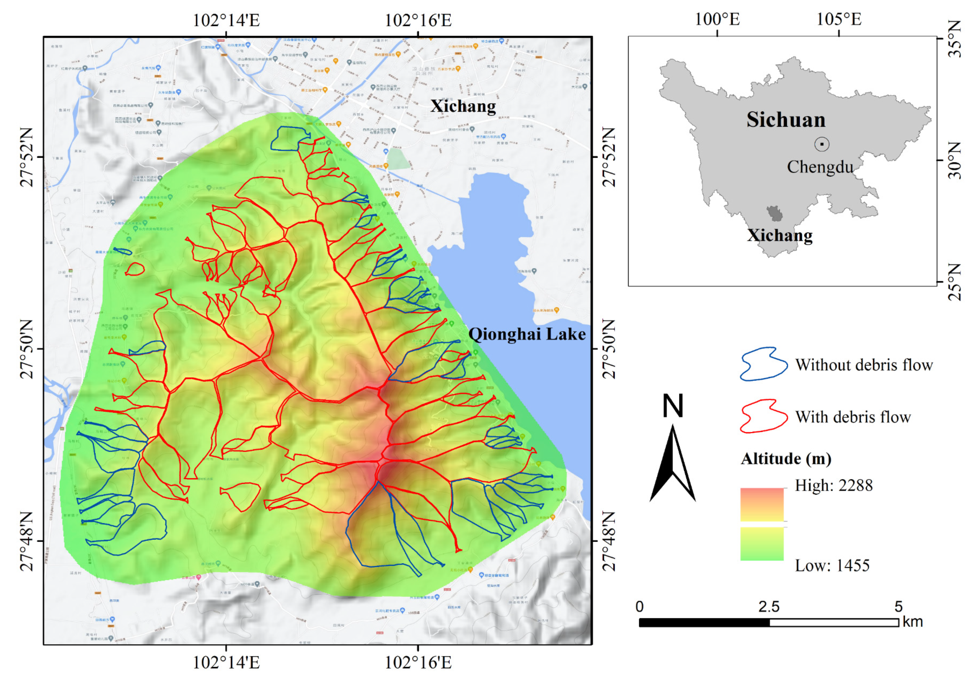
2. Study Area
2.1. Geological Settings
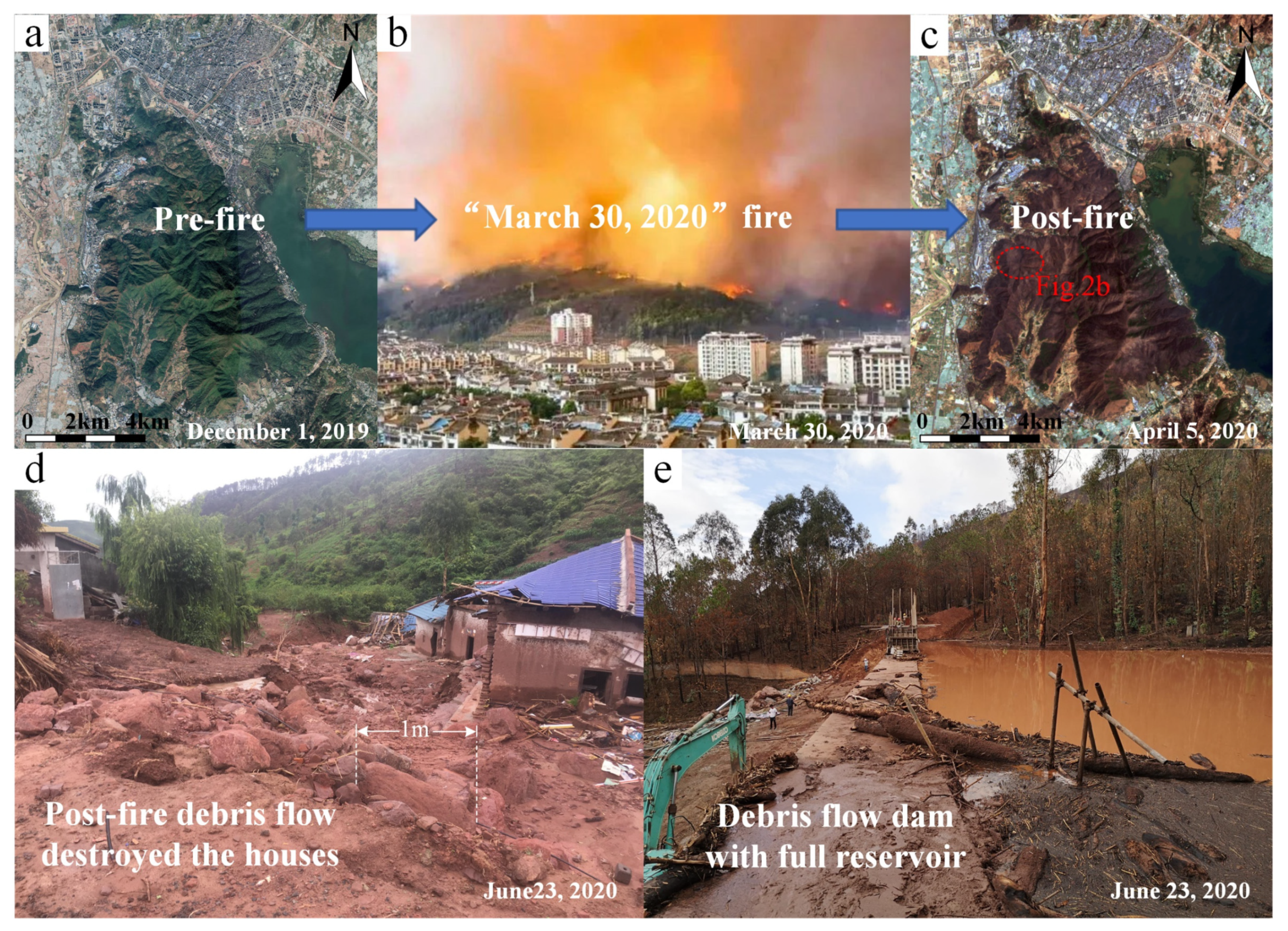
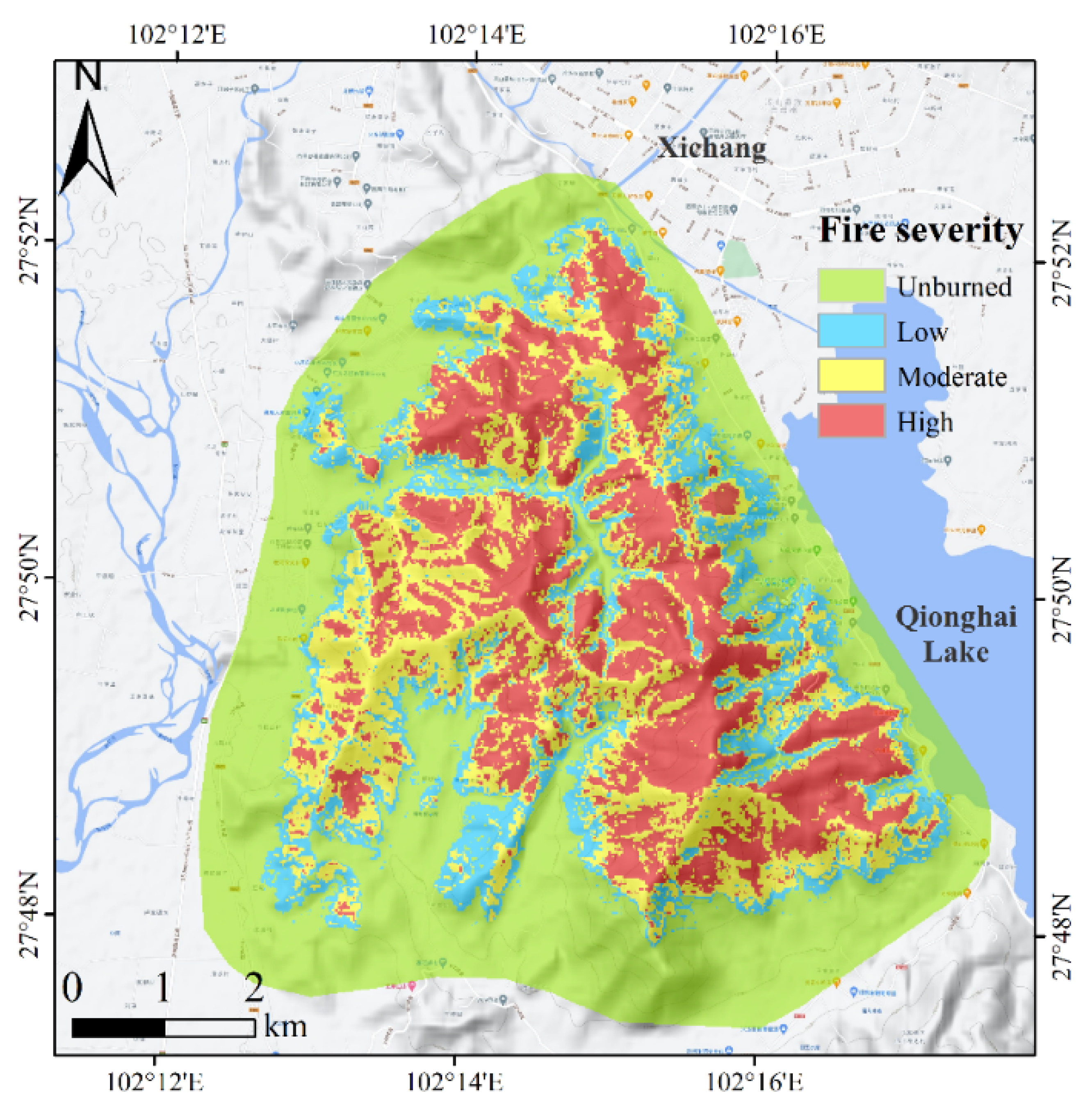
2.2. Thirtith March 2020 Forest Fire and Post-Fire Debris-Flow Events
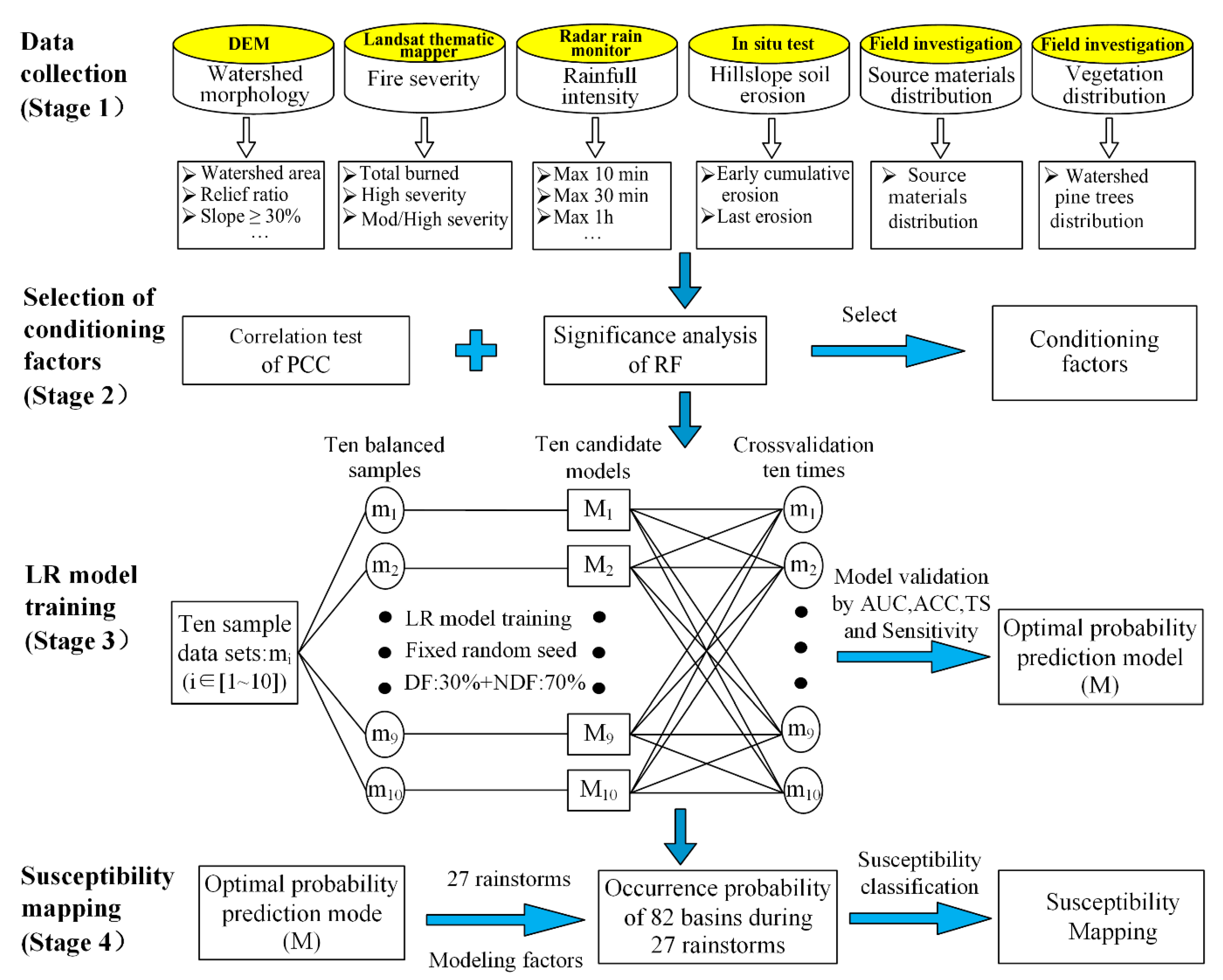
3. Materials and Methods
3.1. Database preparation
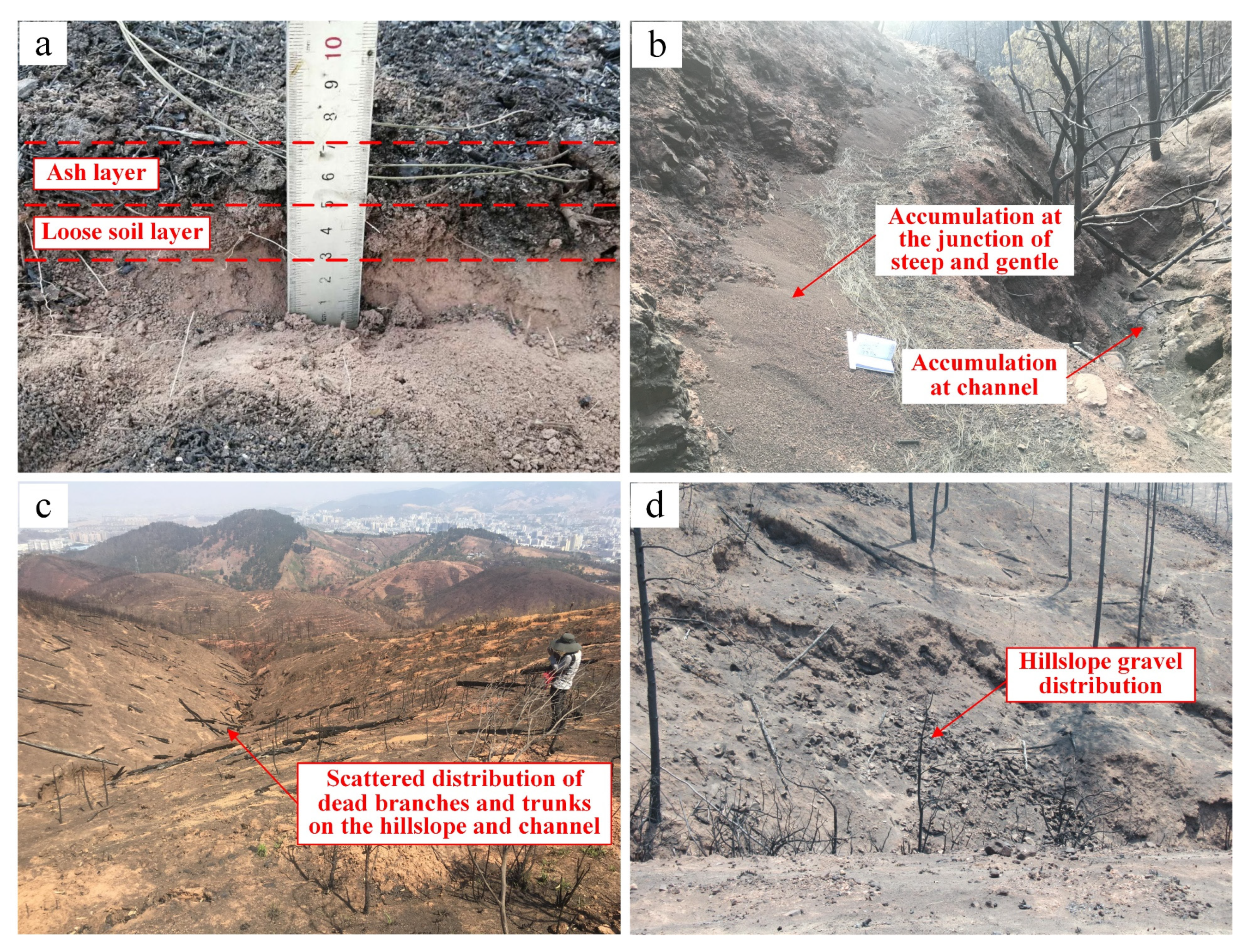
3.1.1. Post-Fire Debris Flow Inventory
3.1.2. Post-Fire Debris Flow Conditioning Factors
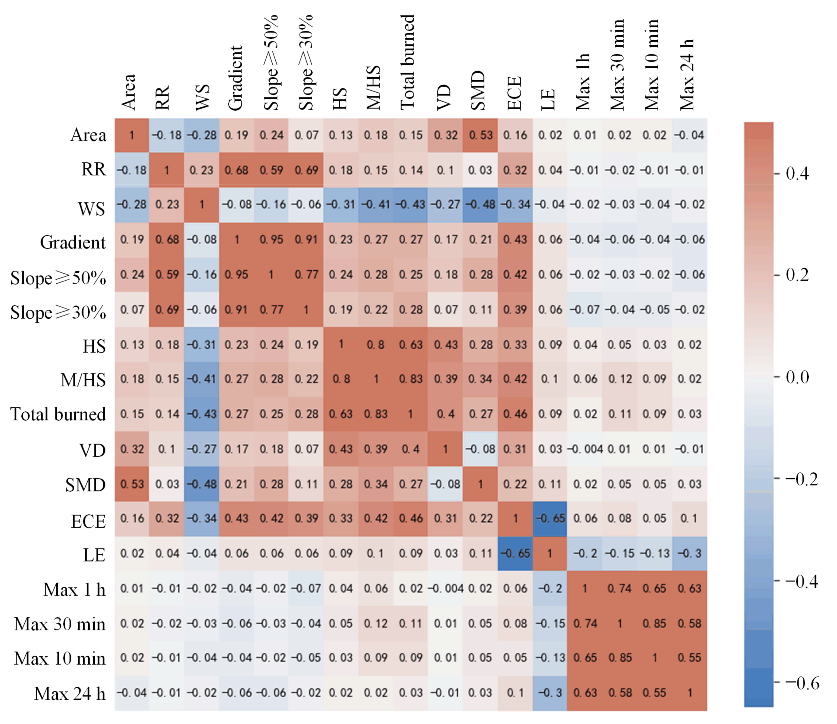
3.2. Selecting the Post-Fire Debris Flow Conditioning Factors
3.3. Model
3.4. Model Training and Validation
4. Results
4.1. Modeling Factor Selection
4.2. Optimal Probability Prediction Model Selection
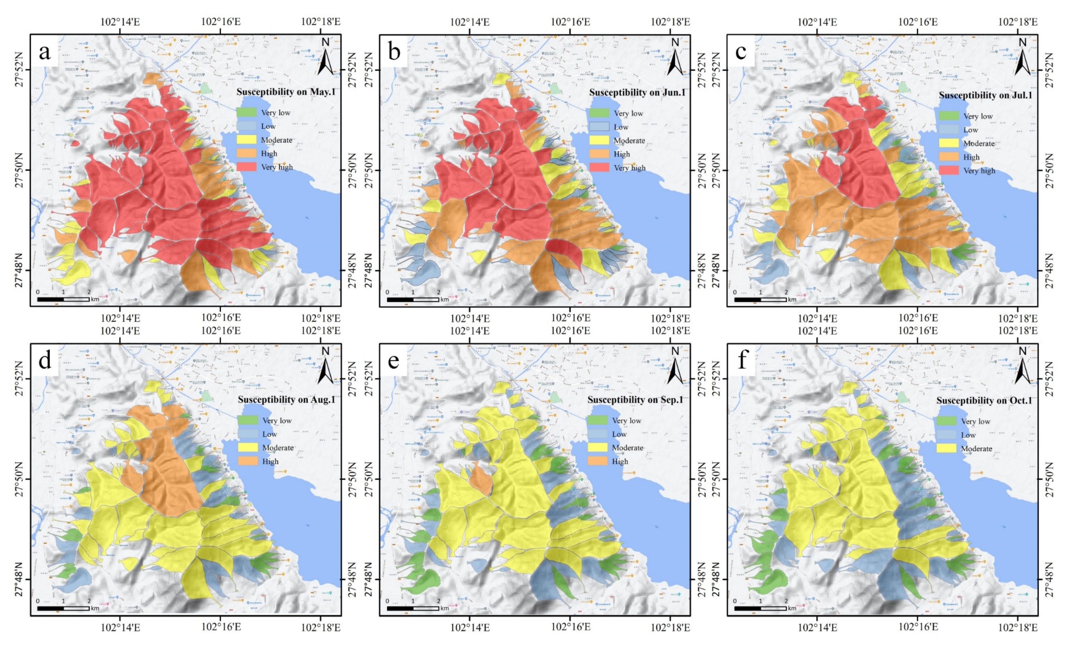
4.3. Susceptibility Mapping
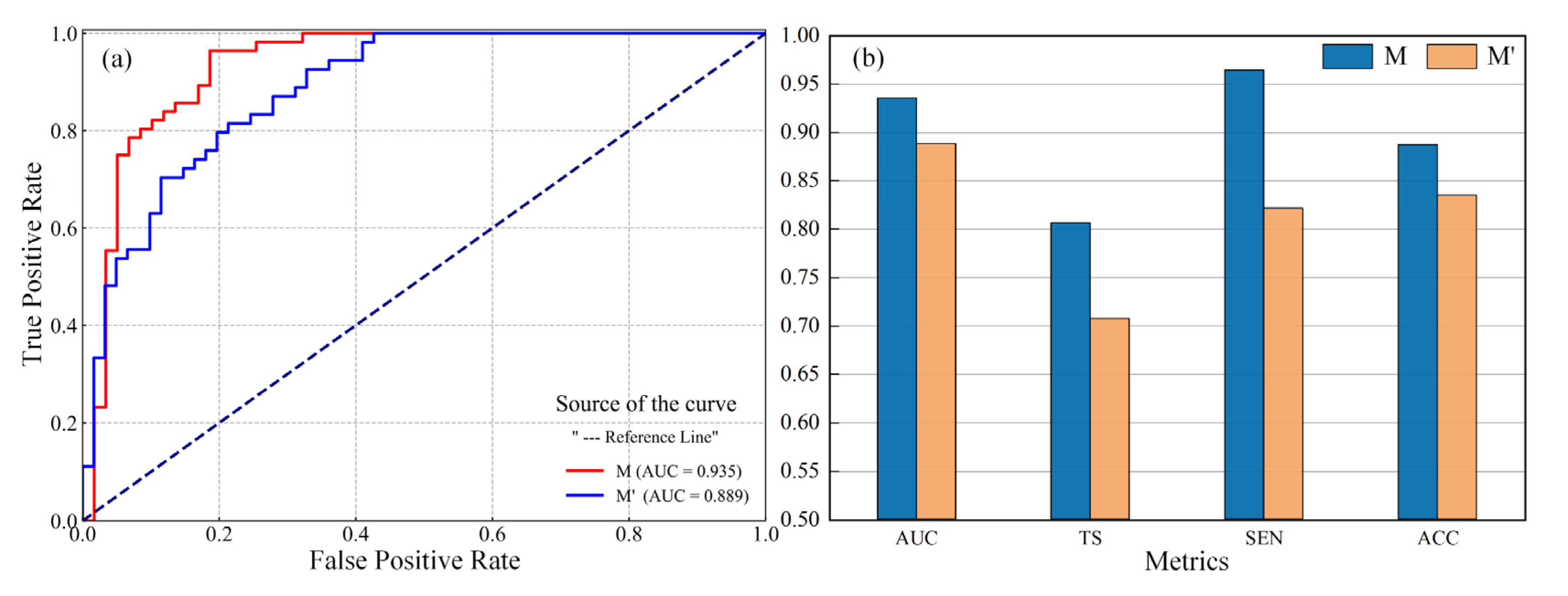
4.4. Validation of Susceptibility Evaluation Results
5. Discussion
6. Conclusions
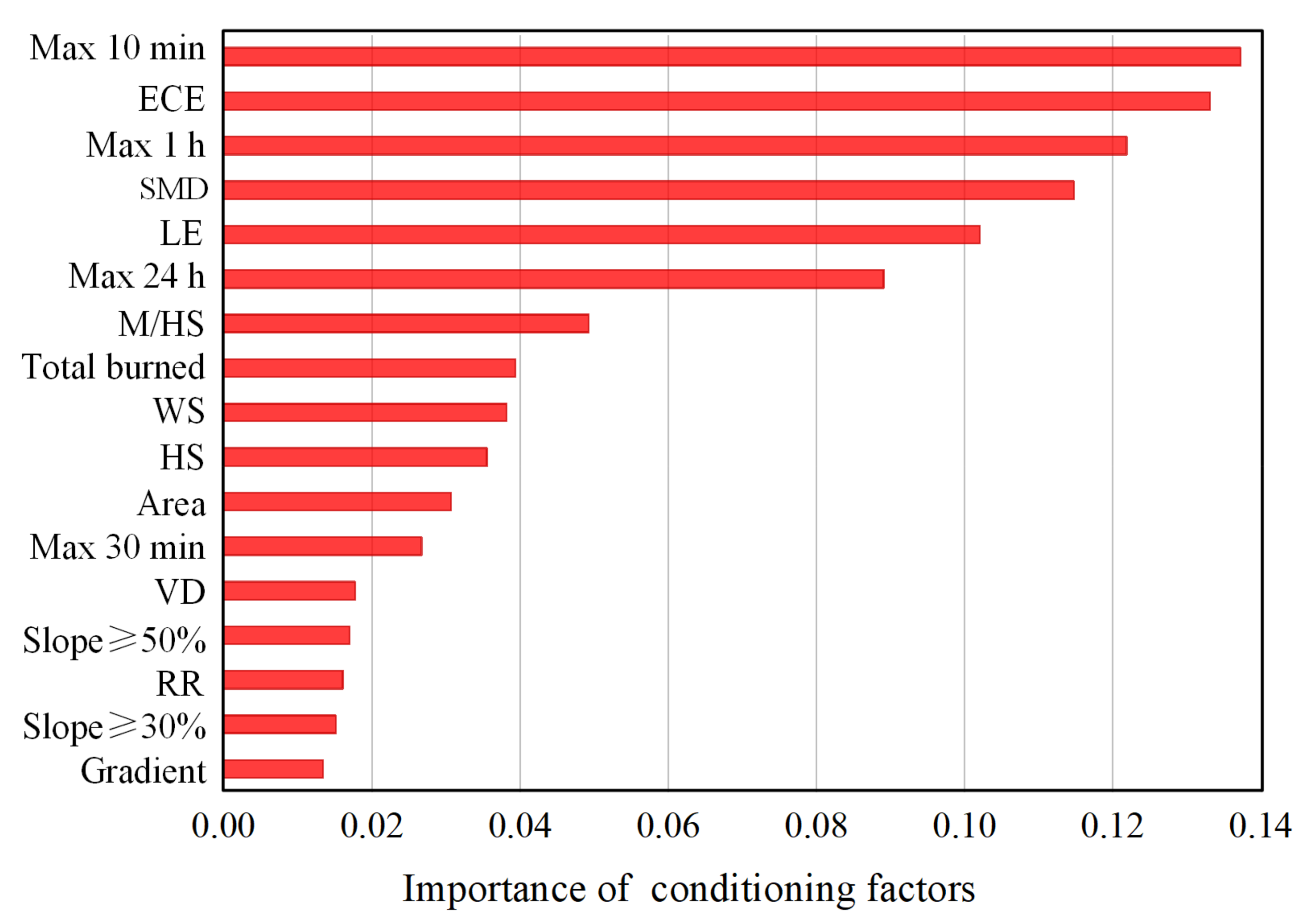
- (1)
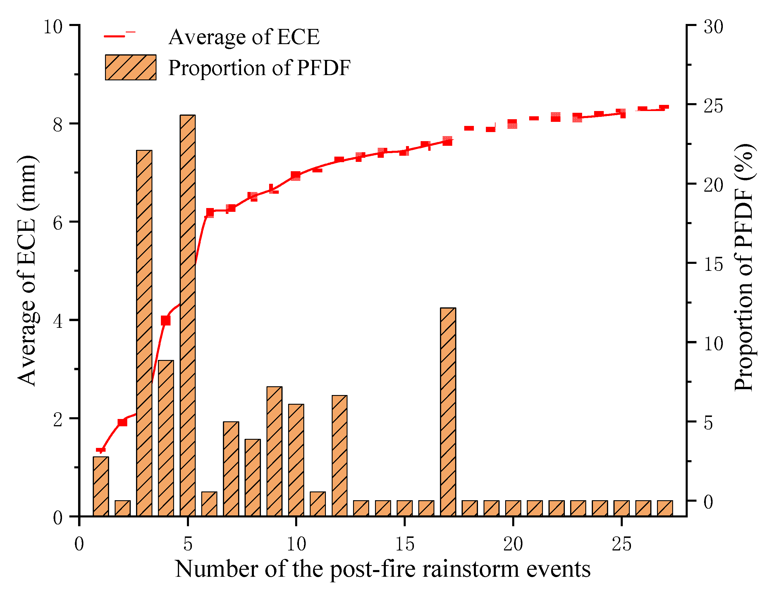
- Max 10 min is the primary factor impacting the initiation of post-fire debris flow (weight: 0.1375), ECE (0.1334), SMD (0.1150), and M/HS (0.0494) are the primary controlling factors affecting the initiation of post-fire debris flow except for rainfall.
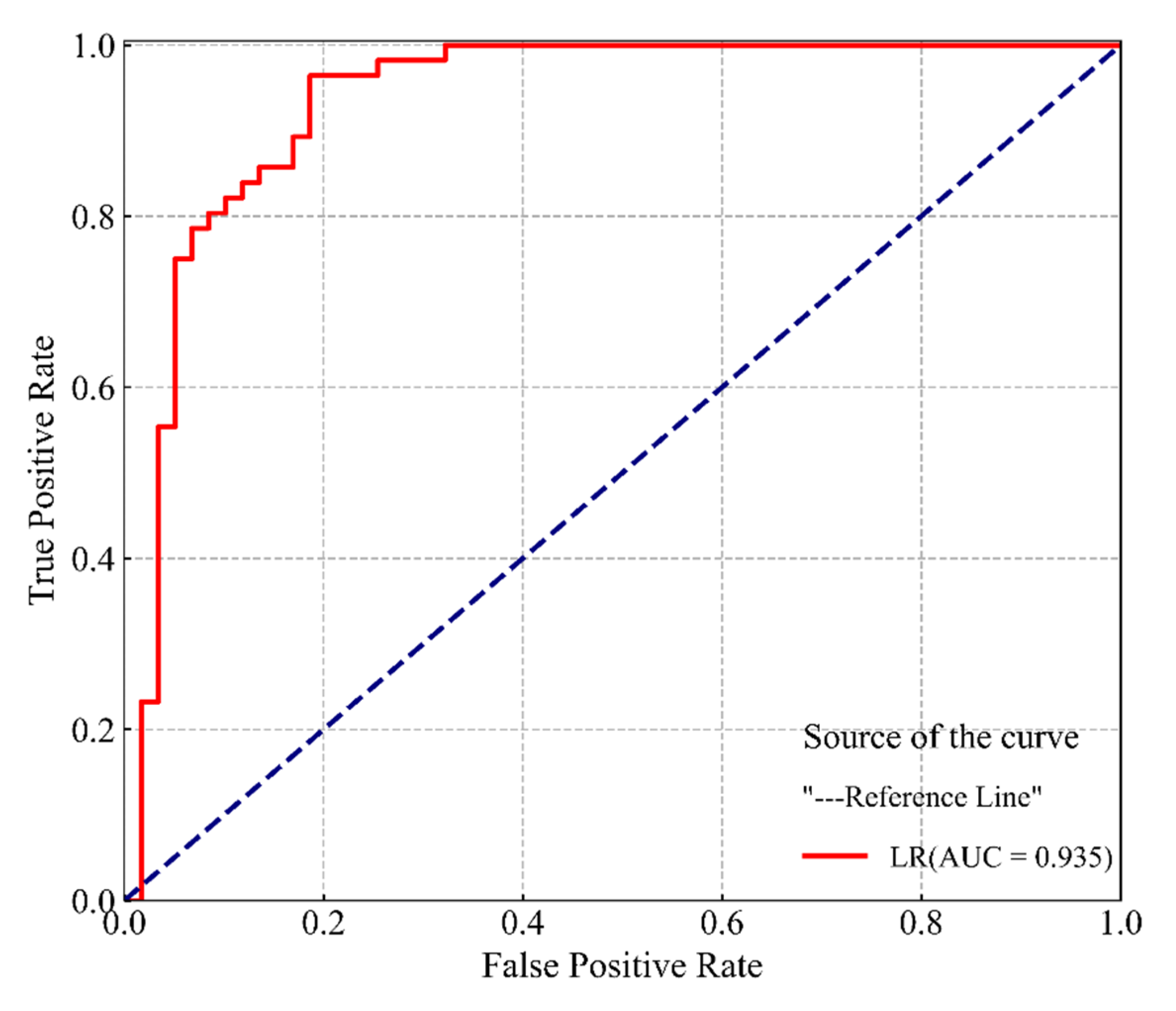
- (2)
- The validation results show that the LR has good prediction performance, in which the AUC is 0.935, the Sensitivity is 0.964, the Accuracy is 0.887, and the TS is 0.806.
- (3)
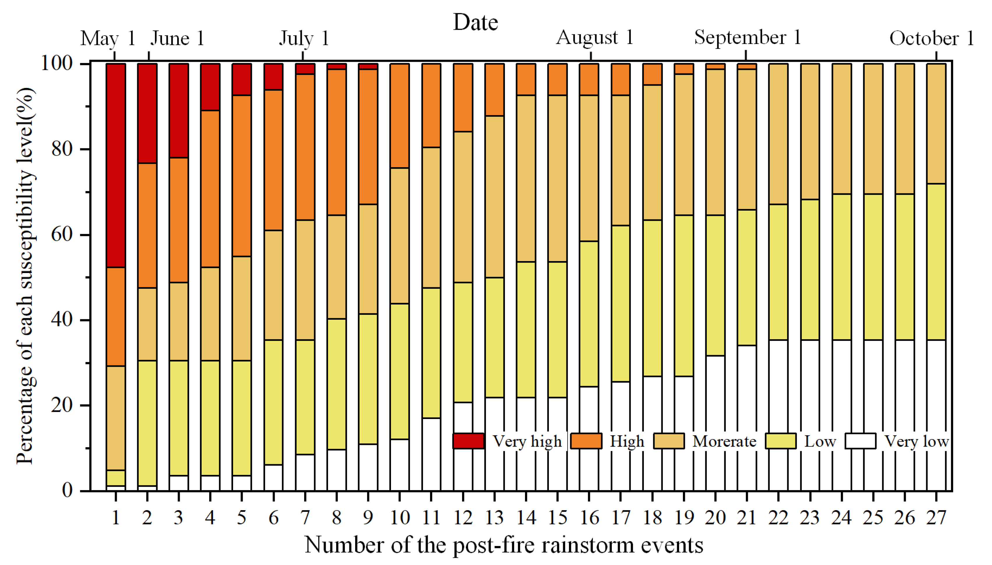
- The susceptibility of PFDF has significantly reduced over time. After two months of wildfire, the proportions of very low, low, moderate, high, and very high susceptibility are 1.2%, 3.7%, 24.4%, 23.2%, and 47.6%, respectively. After seven months of wildfire, the proportions of high and very high susceptibility decreased to 0, while the proportions of very low to medium susceptibility increased to 35.4%, 35.6%, and 28.1%, respectively.
- (4)
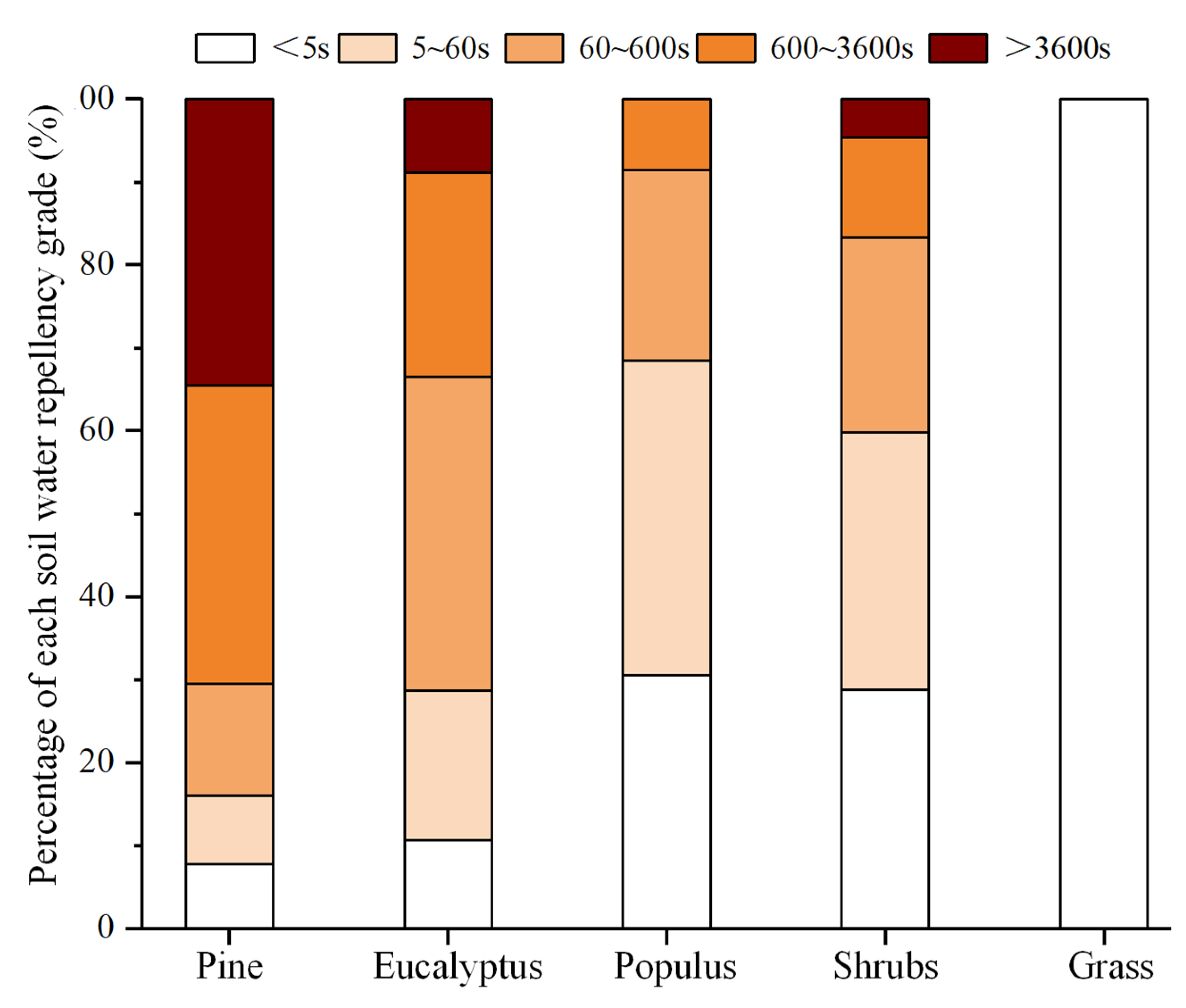
- Human activity plays an important role in the recovery of watersheds after the wildfire. The drone seeding of grass seeds and artificial planting of trees accelerated the natural recovery of vegetation and soil, which significantly reduced the duration of PFDF disasters in the study area.
Author Contributions
Funding
Data Availability Statement
Acknowledgments
Conflicts of Interest
References
- Wall, S.A.; Roering, J.J.; Rengers, F.K. Runoff-initiated post-fire debris flow Western Cascades, Oregon. Landslides 2020, 17, 1649–1661. [Google Scholar] [CrossRef]
- Thomas, M.A.; Rengers, F.K.; Kean, J.W.; Mcguire, L.A.; Ebel, B.A. Postwildfire soil-hydraulic recovery and the persistence of debris flow hazards. J. Geophys. Res. Earth Surf. 2021, 126, e2021JF006091. [Google Scholar] [CrossRef]
- Lancaster, J.T.; Swanson, B.J.; Lukashov, S.G.; Oakley, N.S.; Lee, J.B.; Spangler, E.R. Observations and analyses of the 9 January 2018 debris-flow disaster, Santa Barbara County, California. Environ. Eng. Geosci. 2021, 27, 3–27. [Google Scholar] [CrossRef]
- Shakesby, R.A.; Doerr, S.H. Wildfire as a hydrological and geomorphological agent. Earth-Sci. Rev. 2006, 74, 269–307. [Google Scholar] [CrossRef]
- Diakakis, M. Flood seasonality in Greece and its comparison to seasonal distribution of flooding in selected areas across southern Europe. J. Flood Risk Manag. 2017, 10, 30–41. [Google Scholar] [CrossRef]
- Addison, P.; Oommen, T. Post-fire debris flow modeling analyses: Case study of the post-Thomas Fire event in California. Nat. Hazards 2020, 100, 329–343. [Google Scholar] [CrossRef] [Green Version]
- Cannon, S.H.; Gartner, J.E.; Rupert, M.G.; Michael, J.A.; Rea, A.H.; Parrett, C. Predicting the probability and volume of postwildfire debris flows in the intermountain western United States. Geol. Soc. Am. Bull. 2010, 122, 127–144. [Google Scholar] [CrossRef]
- Staley, D.M.; Negri, J.A.; Kean, J.W.; Laber, J.L.; Tillery, A.C.; Youberg, A.M. Prediction of spatially explicit rainfall intensity–duration thresholds for post-fire debris-flow generation in the western United States. Geomorphology 2017, 278, 149–162. [Google Scholar] [CrossRef]
- Napoli, M.D.; Marsiglia, P.; Martire, D.D.; Ramondini, M.; Calcaterra, D. Landslide susceptibility assessment of wildfire burnt areas through earth-observation techniques and a machine learning-based approach. Remote Sens. 2020, 12, 2505. [Google Scholar] [CrossRef]
- Nikolopoulos, E.I.; Destro, E.; Bhuiyan, M.A.E.; Borga, M.; Anagnostou, E.N. Evaluation of predictive models for post-fire debris flows occurrence in the western United States. Nat. Hazards Earth Syst. Sci. Discuss. 2018, 18, 2331–2343. [Google Scholar] [CrossRef] [Green Version]
- Cannon, S.H.; Powers, P.S.; Savage, W.Z. Fire-related hyperconcentrated and debris flows on Storm King Mountain, Glenwood Springs, Colorado, USA. Environ. Geol. 1998, 35, 210–218. [Google Scholar] [CrossRef]
- Hu, X.W.; Wang, Y.; Yang, Y. Research actuality and evolution mechanism of post-fire debris flow. J. Eng. Geol. 2018, 26, 1562–1573. [Google Scholar]
- Cannon, S.H. Debris-flow generation from recently burned watersheds. Environ. Eng. Geosci. 2001, 7, 321–341. [Google Scholar] [CrossRef]
- Gartner, J.E.; Cannon, S.H.; Bigio, E.R.; Davis, N.K.; Parrett, C.; Pierce, K.L.; Rupert, M.G.; Thurston, B.L.; Trebish, M.J.; Garcia, S.P. Compilation of data relating to the erosive respose of 606 recently-burned basins in the Western United States. US Geol. Surv. Open-File Rep. 2005, 1218. Available online: https://pubs.usgs.gov/of/2005/1218/ (accessed on 1 March 2022).
- Nyman, P.; Sheridan, G.J.; Smith, H.G.; Lane, P. Evidence of debris flow occurrence after wildfire in upland catchments of south-east Australia. Geomorphology 2011, 125, 383–401. [Google Scholar] [CrossRef]
- Nyman, P.; Smith, H.G.; Sherwin, C.B.; Langhans, C.; Lane, P.; Sheridan, G.J. Predicting sediment delivery from debris flows after wildfire. Geomorphology 2015, 250, 173–186. [Google Scholar] [CrossRef]
- Hu, X.W.; Jin, T.; Yin, W.Q.; Huo, Z.B.; Song, Y.P.; Zhang, S.K.; Wang, Y.; Yang, Y. The characteristics of forest fire burned area and susceptibility assessment of post-fire debris flow in Jingjiu Township, Xichang City. J. Eng. Geol. 2020, 28, 762–771, (In Chinese with English abstract). [Google Scholar]
- Flannigan, M.D.; Krawchuk, M.A.; De Groot, W.J.; Wotton, B.M.; Gowman, L.M. Implications of changing climate for global wildland fire. Int. J. Wildland Fire 2009, 18, 483–507. [Google Scholar] [CrossRef]
- Westerling, A.L.; Hidalgo, H.G.; Cayan, D.R.; Swetnam, T.W. Warming and earlier spring increase western US forest wildfire activity. Science 2006, 313, 940–943. [Google Scholar] [CrossRef] [Green Version]
- Oakley, N.S. A Warming Climate Adds Complexity to Post-Fire Hydrologic Hazard Planning. Earth’s Future 2021, 9, e2021EF002149. [Google Scholar] [CrossRef]
- Jin, T.; Hu, X.W.; Xi, C.J.; He, K.; Yang, Y.; Cao, X.C. Susceptibility assessment of “2020.3.30” Xichang post-fire debris flow using a machine learning method. IOP Conf. Ser. Earth Environ. Sci. 2021, 861, 062039. [Google Scholar] [CrossRef]
- Wang, Y.; Hu, X.W.; Jin, T.; Yang, Y.; Cao, X.C. Material initiation of debris flow generation processes after hillside fires. J. Eng. Geol. 2019, 27, 1415–1423. [Google Scholar]
- Yang, Y.; Hu, X.W.; Wang, Y.; Jin, T.; Cao, X.C.; Han, M. Spatial Development Characteristics of Post-Fire Debris Flow in Ba-jiaolou Town. J. Southwest Jiaotong Univ. 2021, 56, 818–827. [Google Scholar]
- Santi, P.M.; Rengers, F.K. Wildfire and landscape change. In Reference Module in Earth Systems and Environmental Sciences; Elsevier: Amsterdam, The Netherlands, 2020. [Google Scholar] [CrossRef]
- Hoch, O.J.; McGuire, L.A.; Youberg, A.M.; Rengers, F.K. Hydrogeomorphic Recovery and Temporal Changes in Rainfall Thresholds for Debris Flows Following Wildfire. J. Geophys. Res. Earth Surf. 2021, 126, e2021JF006374. [Google Scholar] [CrossRef]
- Parsons, A.; Robichaud, P.R.; Lewis, S.A.; Napper, C.; Clark, J.T. Field Guide for Mapping Post-Fire Soil Burn Severity; Gen. Tech. Rep. RMRS-GTR-243; U.S. Department of Agriculture, Forest Service, Rocky Mountain Research Station: Fort Collins, CO, USA, 2010; Volume 243, p. 49. Available online: https://www.fs.usda.gov/treesearch/pubs/36236 (accessed on 1 March 2022).
- Moody, J.A.; Martin, D.A. Initial hydrologic and geomorphic response following a wildfire in the Colorado Front Range. Earth Surf. Process. Landf. 2001, 26, 1049–1070. [Google Scholar] [CrossRef]
- Moody, J.A.; Ebel, B.A. Infiltration and runoff generation processes in fire-affected soils. Hydrol. Process. 2014, 28, 3432–3453. [Google Scholar] [CrossRef]
- Ebel, B.A.; Martin, D.A. Meta-analysis of field-saturated hydraulic conductivity recovery following wildland fire: Applications for hydrologic model parameterization and resilience assessment. Hydrol. Process. 2017, 31, 3682–3696. [Google Scholar] [CrossRef]
- Kean, J.W.; Staley, D.M.; Lancaster, J.T.; Rengers, F.K.; Swanson, B.J.; Coe, J.A.; Hernandez, J.L.; Sigman, A.J.; Allstadt, K.E.; Lindsay, D.N. Inundation, flow dynamics, and damage in the 9 January 2018 Montecito debris-flow event, California, USA: Opportunities and challenges for post-wildfire risk assessment. Geosphere 2019, 15, 1140–1163. [Google Scholar] [CrossRef] [Green Version]
- Raymond, C.A.; McGuire, L.A.; Youberg, A.M.; Staley, D.M.; Kean, J.W. Thresholds for post wildfire debris flows: Insights from the Pinal Fire, Arizona, USA. Earth Surf. Process. Landf. 2020, 45, 1349–1360. [Google Scholar] [CrossRef]
- Weninger, T.; Filipović, V.; Mešić, M.; Clothier, B.; Filipović, L. Estimating the extent of fire induced soil water repellency in Mediterranean environment. Geoderma 2019, 338, 187–196. [Google Scholar] [CrossRef]
- DeGraff, J.V. Improvement in quantifying debris flow risk for post-wildfire emergency response. Geoenviron. Disasters 2014, 1, 5. [Google Scholar] [CrossRef] [Green Version]
- Gartner, J.E.; Cannon, S.H.; Helsel, D.R.; Bandurraga, M. Multivariate Statistical Models for Predicting Sediment Yields from Southern California Watersheds. U. S. Geol. Surv. Open-File Rep. 2009, 1200, 42. Available online: https://citeseerx.ist.psu.edu/viewdoc/download?doi=10.1.1.593.192&rep=rep1&type=pdf (accessed on 1 March 2022).
- McGuire, L.A.; Youberg, A.M. What drives spatial variability in rainfall intensity-duration thresholds for post-wildfire debris flows? Insights from the 2018 Buzzard Fire, NM, USA. Landslides 2020, 17, 2385–2399. [Google Scholar] [CrossRef]
- Liu, T.; Mcguire, L.A.; Wei, H.; Rengers, F.K.; Gupta, H.; Ji, L.; Goodrich, D.C. The timing and magnitude of changes to Hortonian overland flow at the watershed scale during the post-fire recovery process. Hydrol. Process. 2021, 35, e14208. [Google Scholar] [CrossRef]
- Staley, D.M.; Gartner, J.E.; Smoczyk, G.M.; Reeves, R.R. Emergency assessment of post-fire debris-flow hazards for the 2013 Mountain fire, southern California. U. S. Geol. Surv. Open-File Rep. 2013, 1249, 13. Available online: https://pubs.usgs.gov/of/2013/1249/ (accessed on 1 March 2022).
- Cannon, S.H.; Gartner, J.E.; Wilson, R.; Bowers, J.; Laber, J. Storm rainfall conditions for floods and debris flows from recently burned areas in southwestern Colorado and southern California. Geomorphology 2008, 96, 250–269. [Google Scholar] [CrossRef]
- Ren, Y.; Hu, X.W.; Wang, Y.; Yang, Y. Disaster mechanism of the Sejiao post-fire debris flow in Jiulong County of Sichuan. Hydrogeol. Eng. Geol. 2018, 45, 150–156. [Google Scholar]
- Johnson, P.A.; McCuen, R.H.; Hromadka, T.V. Magnitude and frequency of debris flows. J. Hydrol. 1991, 123, 69–82. [Google Scholar] [CrossRef]
- Hungr, O.; Morgan, G.C.; Kellerhals, R. Quantitative analysis of debris torrent hazards for design of remedial measures. Can. Geotech. J. 1984, 21, 663–677. [Google Scholar] [CrossRef]
- Kern, A.N.; Addison, P.; Oommen, T.; Salazar, S.E.; Coffman, R.A. Machine learning based predictive modeling of debris flow probability following wildfire in the intermountain Western United States. Math. Geosci. 2017, 49, 717–735. [Google Scholar] [CrossRef]
- Addison, P.; Addison, P.; Oommen, T. Assessment of post-wildfire debris flow occurrence using classifier tree. Geomat. Nat. Haz. Risk. 2019, 10, 505–518. [Google Scholar] [CrossRef] [Green Version]
- Rupert, M.G.; Cannon, S.H.; Gartner, J.E.; Michael, J.A.; Helsel, D.R. Using logistic regression to predict the probability of debris flows in areas burned by wildfires, southern California, 2003–2006. U. S. Geol. Surv. Open-File Rep. 2008, 1370, 9. Available online: https://pubs.usgs.gov/of/2008/1370/ (accessed on 1 March 2022).
- Staley, D.M.; Negri, J.A.; Kean, J.W.; Laber, J.L.; Tillery, A.C.; Youberg, A.M. Updated Logistic Regression Equations for the Calculation of Post-Fire Debris-Flow Likelihood in the Western United States. U. S. Geol. Surv. Open-File Rep. 2016, 1106, 13. Available online: https://pubs.usgs.gov/of/2016/1106/ofr20161106 (accessed on 1 March 2022).
- Wang, X.; Wang, R.T. Temporal and Spatial Characteristics of Forest Fire in Sichuan and Its Climate Background. Chin. Agric. Sci. Bull. 2014, 30, 155–160, (In Chinese with English abstract). [Google Scholar]
- Pierson, T.C. Distinguishing between Debris Flows and Floods from Field Evidence in Small Watersheds. U. S. Geol. Surv. Fact Sheet. 2005, 2004–3142, 4. Available online: https://pubs.er.usgs.gov/publication/fs20043142 (accessed on 1 March 2022).
- Gabet, E.J. Post-fire thin debris flows: Sediment transport and numerical modelling. Earth Surf. Process. Landf. 2003, 28, 1341–1348. [Google Scholar] [CrossRef]
- Kean, J.W.; Staley, D.M.; Cannon, S.H. In situ measurements of post-fire debris flows in southern California: Comparisons of the timing and magnitude of 24 debris-flow events with rainfall and soil moisture conditions. J. Geophys. Res. Earth Surf. 2011, 116, F04019. [Google Scholar] [CrossRef]
- Hyde, K.D.; Wilcox, A.C.; Jencso, K. Effects of vegetation disturbance by fire on channel initiation thresholds. Geomorphology 2014, 214, 84–96. [Google Scholar] [CrossRef]
- Mitsopoulos, I.D.; Mironidis, D. Assessment of post fire debris flow potential in a Mediterranean type ecosystem. Wit Trans. Ecol. Environ. 2006, 90, 221–229. [Google Scholar]
- Key, C.H.; Benson, N.C. Landscape Assessment: Ground Measure Severity, the Composite Burn Index; and Remote Sensing of Severity, the Normalized Burn Ratio; RMRS-GTR-164-CD; U.S. Department of Agriculture-Forest Service, Rocky Mountain Research Station: Fort Collins, CO, USA, 2006; pp. 1–51. Available online: https://pubs.er.usgs.gov/publication/2002085 (accessed on 1 March 2022).
- Miller, J.D.; Thode, A.E. Quantifying burn severity in a heterogeneous landscape with a relative version of the delta Normalized Burn Ratio (dNBR). Remote Sens. Environ. 2007, 109, 66–80. [Google Scholar] [CrossRef]
- Wang, Y.; Hu, X.W.; Yang, Y.; Yu, Z.J.; Cao, X.C. Research on the change in soil water repellency and permeability in burned areas. Hydrogeol. Eng. Geol. 2019, 46, 40–45. [Google Scholar]
- Fassnacht, F.E.; Schmidt-Riese, E.; Kattenborn, T.; Hernandez, J. Explaining sentinel 2-based dNBR and RdNBR variability with reference data from the bird’s eye (USA) perspective. Int. J. Appl. Earth Obs. Geoinf. 2021, 95, 102262. [Google Scholar] [CrossRef]
- Mousivand, A.; Verhoef, W.; Menenti, M.; Gorte, B. Modeling top of atmosphere radiance over heterogeneous non-Lambertian rugged terrain. Remote Sens. 2015, 7, 8019–8044. [Google Scholar] [CrossRef] [Green Version]
- Kean, J.W.; Staley, D.M.; Leeper, R.J.; Schmidt, K.M. A low-cost method to measure the timing of post-fire flash floods and debris flows relative to rainfall. Water Resour. Res. 2012, 48, W05516. [Google Scholar] [CrossRef]
- Staley, D.M.; Kean, J.W.; Cannon, S.H.; Schmidt, K.M.; Laber, J.L. Objective definition of rainfall intensity–duration thresholds for the initiation of post-fire debris flows in southern California. Landslides 2013, 10, 547–562. [Google Scholar] [CrossRef]
- Yang, P.; Liu, X.H.; Liang, S.X. The application of the mathematical model of Distance Weighted Mean to rainfall isoline in Haihe River Basin. Hydrology 2003, 23, 42–45. [Google Scholar]
- Wohlgemuth, P.M.; Hubbert, K.R.; Robichaud, P.R. The effects of log erosion barriers on post-fire hydrologic response and sediment yield in small forested watersheds, southern California. Hydrol. Process. 2001, 15, 3053–3066. [Google Scholar] [CrossRef]
- McGuire, L.A.; Kean, J.W.; Staley, D.M.; Rengers, F.K.; Wasklewicz, T.A. Constraining the relative importance of raindrop and flow driven sediment transport mechanisms in post-wildfire environments and implications for recovery time scales. J. Geophys. Res. Earth Surf. 2016, 121, 2211–2237. [Google Scholar] [CrossRef] [Green Version]
- Neary, D.G.; Klopatek, C.C.; Debano, L.F.; Ffolliott, P.F. Fire effects on belowground sustainability: A review and synthesis. For. Ecol. Manag. 1999, 122, 51–71. [Google Scholar] [CrossRef]
- Yang, Y.; Hu, X.W.; Wang, Y.; Jin, T.; Cao, X.C.; Han, M. Preliminary study on the methods to calculate the dynamic reserves of slope erosioning materials transported by the post-fire debris flow. J. Eng. Geol. 2021, 29, 151–161. [Google Scholar]
- Staley, D.M.; Wasklewicz, T.A.; Kean, J.W. Characterizing the primary material sources and dominant erosional processes for post-fire debris-flow initiation in a headwater basin using multi-temporal terrestrial laser scanning data. Geomorphology 2014, 214, 324–338. [Google Scholar] [CrossRef]
- Tang, H.; McGuire, L.A.; Rengers, F.K.; Kean, J.W.; Staley, D.M.; Smith, J.B. Evolution of debris-flow initiation mechanisms and sediment sources during a sequence of postwildfire rainstorms. J. Geophys. Res. Earth Surf. 2019, 124, 1572–1595. [Google Scholar] [CrossRef] [Green Version]
- DiBiase, R.A.; Lamb, M.P. Dry sediment loading of headwater channels fuels post-wildfire debris flows in bedrock landscapes. Geology 2020, 48, 189–193. [Google Scholar] [CrossRef] [Green Version]
- Gabet, E.J.; Sternberg, P. The effects of vegetative ash on infiltration capacity, sediment transport, and the generation of progressively bulked debris flows. Geomorphology 2008, 101, 666–673. [Google Scholar] [CrossRef]
- Ministry of Land and Resources of the People’s Republic of China 2006 Specification of Geological Investigation for Debris Flow Stabilization: DZ/T 0220-2006; Standards Press of China: Beijing, China, 2006. (In Chinese)
- Badía, D.; Aguirre, J.A.; Martí, C.; Márquez, M.A. Sieving effect on the intensity and persistence of water repellency at different soil depths and soil types from ne-spain. Catena 2013, 108, 44–49. [Google Scholar] [CrossRef]
- Doerr, S.H.; Shakesby, R.S.; Walsh, R.P.D. Spatial variability of soil hydrophobicity in fire-prone eucalyptus and pine forests, Portugal. Soil Sci. 1998, 163, 313–324. [Google Scholar] [CrossRef]
- Breiman, L. Random forests. Mach. Learn. 2001, 45, 5–32. [Google Scholar] [CrossRef] [Green Version]
- Wang, Y.M.; Feng, L.W.; Li, S.J.; Ren, F.; Du, Q.Y. A hybrid model considering spatial heterogeneity for landslide susceptibility mapping in Zhejiang Province, China. Catena 2020, 188, 104425. [Google Scholar] [CrossRef]
- Boulesteix, A.L.; Bender, A.; Lorenzo Bermejo, J.; Strobl, C. Random forest Gini importance favours SNPs with large minor allele frequency: Impact, sources and recommendations. Brief. Bioinform. 2012, 13, 292–304. [Google Scholar] [CrossRef] [Green Version]
- Gartner, J.E.; Cannon, S.H.; Santi, P.M.; Dewolfe, V. Empirical models to predict the volumes of debris flows generated by recently burned basins in the western U.S. Geomorphology 2008, 96, 339–354. [Google Scholar] [CrossRef]
- Gartner, J.E.; Cannon, S.H.; Santi, P.M. Empirical models for predicting volumes of sediment deposited by debris flows and sediment-laden floods in the transverse ranges of southern California. Eng. Geol. 2014, 176, 45–56. [Google Scholar] [CrossRef]
- Kotsiantis, S.; Kannellopoulos, D.; Pintelas, P. Data preprocessing for supervised learning. Int. J. Comput. Sci. 2006, 1, 111–117. [Google Scholar]
- Schaefer, J.T. The critical success index as an indicator of warning skill. Weather Forecast. 1990, 5, 570–575. [Google Scholar] [CrossRef] [Green Version]
- Prosser, I.P.; Williams, L. The effect of wildfire on runoff and erosion in native eucalyptus forest. Hydrol. Processes 1998, 12, 251–265. [Google Scholar] [CrossRef]
- Kim, Y.; Kim, C.G.; Lee, K.S.; Choung, Y. Effects of Post-Fire Vegetation Recovery on Soil Erosion in Vulnerable Montane Regions in a Monsoon Climate: A Decade of Monitoring. J. Plant Biol. 2021, 64, 123–133. [Google Scholar] [CrossRef]
- DeGraff, J.V.; Cannon, S.H.; Gartner, J.E. The timing of susceptibility to post-fire debris flows in the Western United States. Environ. Eng. Geosci. 2015, 21, 277–292. [Google Scholar] [CrossRef]
- Guilinger, J.J.; Gray, A.B.; Barth, N.C.; Fong, B.T. The evolution of sediment sources over a sequence of postfire sediment-laden flows revealed through repeat high-resolution change detection. J. Geophys. Res. 2020, 125, e2020JF005527. [Google Scholar] [CrossRef]


| Variable | Description | Source | |
|---|---|---|---|
| Watershed morphology characters | Area (km2) | Watershed area | 12.5 m DEM (ASF, https://search.asf.alaska.edu/, accessed on 12 April 2020) |
| RR (‰) | Relief ratio | ||
| WS | Watershed shape coefficient | ||
| Gradient (°) | Watershed average gradient | ||
| Slope ≥ 30% | Proportion of watershed area with slopes ≥ 30% | ||
| Slope ≥ 50% | Proportion of watershed area with slopes ≥ 50 % | ||
| Fire severity | HS | Proportion of the watershed area burned at high severity | Sentinel-2 data (20 m pixel size) |
| M/HS | Proportion of the watershed area burned at moderate and high severity | ||
| Total burned | Proportion of watershed area that has been burned | ||
| Rainfall intensity | Max 10 min (mm/h) | Maximum 10 min rainfall intensity | Radar rain gauges of Xichang Meteorological Bureau (Every 5 min) |
| Max 30 min (mm/h) | Maximum 30 min rainfall intensity | ||
| Max 1 h (mm/h) | Maximum 1 h rainfall intensity | ||
| Max 24 h (mm) | Maximum 24 h rainfall intensity | ||
| Hillslope soil erosion | ECE (mm) | The cumulative erosion depth of the hillslope soil before the PFDF occurs | Field soil erosion monitoring test (5 months, measured after each rainfall) |
| LE (mm) | The erosion depth of the hillslope soil during the last rainfall | ||
| Source materials distribution | SMD | The ratio of the supply length of the sediment along the main channel in the watershed | Field Investigation (1 m resolution) |
| Vegetation distribution | VD | The original pine tree coverage area in the watershed | Field Investigation (1 m resolution) |
| Fire Severity | Remote Sensing Interpretation (dNBR) | Field Characteristics |
|---|---|---|
| Unburned | <0.12 | There was no change in the surface cover before and after the wildfire |
| Low | 0.12–0.33 | More than 50% of the litter is incompletely burned |
| Moderate | 0.33–0.48 | Most of the litter is burned; however, most of the crude fuel is incompletely burned |
| High | >0.48 | Litter and crude fuel are completely burned and the surface is covered with ashes |
| Observed | |||
|---|---|---|---|
| Debris Flow | No Debris Flow | ||
| Predicted | Debris flow | TP | FP |
| No debris flow | FN | TN | |
| Metrics | AUC | Sensitivity | Accuracy | TS |
|---|---|---|---|---|
| Result | 0.935 | 0.964 | 0.887 | 0.806 |
| Metrics | Balanced Sample Model | Unbalanced Sample Model | D-Value |
|---|---|---|---|
| Sensitivity | 0.878 | 0.259 | 0.619 |
| AUC | 0.922 | 0.907 | 0.015 |
| TS | 0.303 | 0.215 | 0.089 |
| ACC | 0.835 | 0.922 | −0.087 |
| Date | Number of the Post-Fire Rainstorm Events | Very Low (%) | Low (%) | Moderate (%) | High (%) | Very High (%) |
|---|---|---|---|---|---|---|
| 1 May | 1 | 1.22 | 3.66 | 24.39 | 23.17 | 47.56 |
| 1 June | 2 | 1.22 | 29.27 | 17.07 | 29.27 | 23.17 |
| 1 July | 7 | 8.54 | 26.83 | 28.05 | 34.15 | 2.44 |
| 1 August | 16 | 21.95 | 31.71 | 39.02 | 7.32 | 0.00 |
| 1 September | 21 | 34.15 | 31.71 | 32.93 | 1.22 | 0.00 |
| 1 October | 27 | 35.37 | 36.59 | 28.05 | 0.00 | 0.00 |
Publisher’s Note: MDPI stays neutral with regard to jurisdictional claims in published maps and institutional affiliations. |
© 2022 by the authors. Licensee MDPI, Basel, Switzerland. This article is an open access article distributed under the terms and conditions of the Creative Commons Attribution (CC BY) license (https://creativecommons.org/licenses/by/4.0/).
Share and Cite
Jin, T.; Hu, X.; Liu, B.; Xi, C.; He, K.; Cao, X.; Luo, G.; Han, M.; Ma, G.; Yang, Y.; et al. Susceptibility Prediction of Post-Fire Debris Flows in Xichang, China, Using a Logistic Regression Model from a Spatiotemporal Perspective. Remote Sens. 2022, 14, 1306. https://doi.org/10.3390/rs14061306
Jin T, Hu X, Liu B, Xi C, He K, Cao X, Luo G, Han M, Ma G, Yang Y, et al. Susceptibility Prediction of Post-Fire Debris Flows in Xichang, China, Using a Logistic Regression Model from a Spatiotemporal Perspective. Remote Sensing. 2022; 14(6):1306. https://doi.org/10.3390/rs14061306
Chicago/Turabian StyleJin, Tao, Xiewen Hu, Bo Liu, Chuanjie Xi, Kun He, Xichao Cao, Gang Luo, Mei Han, Guotao Ma, Ying Yang, and et al. 2022. "Susceptibility Prediction of Post-Fire Debris Flows in Xichang, China, Using a Logistic Regression Model from a Spatiotemporal Perspective" Remote Sensing 14, no. 6: 1306. https://doi.org/10.3390/rs14061306