
A Femto-Satellite Localization Method Based on TDOA and AOA Using Two CubeSats


1
Space and Planetary Exploration Laboratory (SPEL), Faculty of Physical and Mathematical Sciences, University of Chile, Santiago 8370448, Chile
2
Electrical Enginering Department, Faculty of Physical and Mathematical Sciences, University of Chile, Santiago 8370451, Chile
*
Author to whom correspondence should be addressed.
Remote Sens. 2022, 14(5), 1101; https://doi.org/10.3390/rs14051101
Submission received: 30 November 2021
/
Revised: 21 December 2021
/
Accepted: 27 December 2021
/
Published: 24 February 2022
(This article belongs to the Special Issue CubeSats Applications for Earth and Prospectives for Planetary Remote Sensing)
Abstract
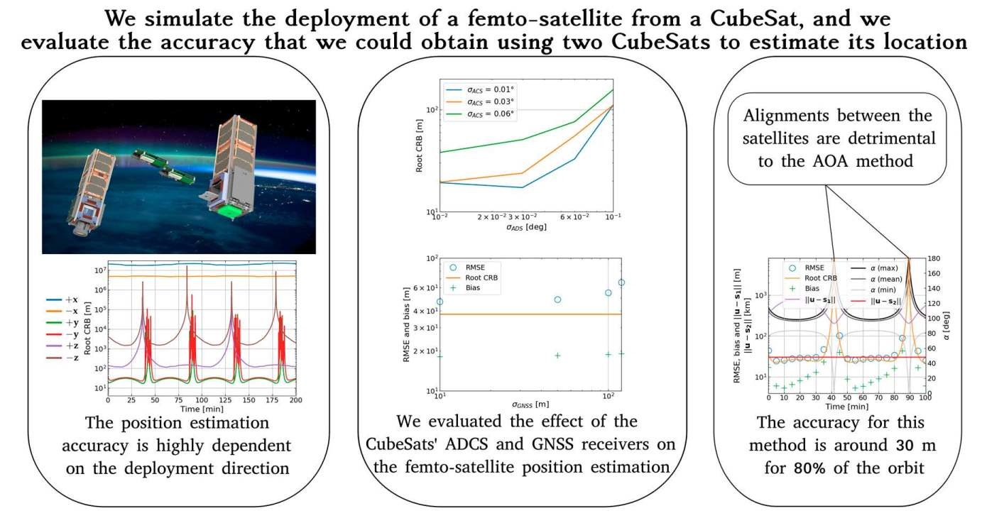
:This article presents a feasibility analysis to remotely estimate the geo-location of a femto-satellite only using two station-CubeSats and the communication link between the femto-satellite and each CubeSat. The presented approach combines the Time Difference Of Arrival (TDOA) and Angle Of Arrival (AOA) methods. We present the motivation, the envisioned solution together with the constraints for reaching it, and the best potential sensitivity of the location precision for different (1) deployment scenarios of the femto-satellite, (2) precisions in the location of the CubeSats, and (3) precisions in each CubeSat’s Attitude Determination and Control Systems (ADCS). We implemented a simulation tool to evaluate the average performance for different random scenarios in space. For the evaluated cases, we found that the Cramér-Rao Bound (CRB) for Gaussian noise over the small error region of the solution is highly dependent on the deployment direction, with differences in the location precision close to three orders of magnitude between the best and worst deployment directions. For the best deployment case, we also studied the best location estimation that might be achieved with the current Global Navigation Satellite System (GNSS) and ADCS commercially available for CubeSats. We found that the mean-square error (MSE) matrix of the proposed solution under the small error condition can attain the CRB for the simulated time, achieving a precision below 30 m when the femto-satellite is separated by around 800 m from the mother-CubeSat.

1. Introduction
Location estimation for satellites is relevant for many reasons, such as establishing the communication with the ground station(s), operating the payload (e.g., imaging over a particular region), and orbital maneuvering, among many others. The location estimation of satellites can be either passive or active. The passive solution requires no action from the satellite to estimate its location. An example of localization systems with passive methods is the use of ground- and space-based (located in other satellites) radars or telescopes. North American Aerospace Defense Command (NORAD) continuously monitors all objects orbiting the Earth with radar installations on the USA and Canada. Leolabs is a company that focuses on the Low Earth Orbit (LEO) and uses phased-array radars to locate the satellites. Neither NORAD nor Leolabs requires the satellite to have special hardware to obtain its position. However, with this method, the satellite is unaware of its position unless it is communicated to it. On the other hand, the active solution requires some action from the satellite to perform the location estimation. The Global Navigation Satellite System (GNSS) and Doppler Orbitography and Radiopositioning Integrated by Satellite (DORIS) [1] are examples of active solutions. The GNSS relies on a satellite network that sends continuous synchronized radio signals to a receiver in the spacecraft, which estimates its location from the multiple received signals. In contrast, DORIS relies on multiple measurements of the Doppler shift of signals sent from ground stations to obtain an accurate estimation.
The reduction in size, time of development, and cost have facilitated the proliferation of a new spectrum of space missions based on satellite constellations or swarms composed of hundreds and even thousands of spacecraft. These spacecraft can be nano-satellites, such as CubeSats, or even femto-satellites carried by CubeSats [2,3]. The potential applications of these constellations are varied, especially for science. Having multiple sensors in space allows researchers to differentiate temporal changes from spatial ones in the measurements. A particular type of mission where this number of spacecraft can be relevant is related to probing the space environment to help understand the impact solar activity has on the ionosphere and the high atmosphere (e.g., [4,5,6]) by using miniaturized sensors in them (e.g., [4,7]). The desired number of satellites required to model the space dynamics usually falls in the hundreds. Moreover, there is a lack of measurements at altitudes below 380 km, where significant propulsion is required to maintain large satellites at those altitudes, making them unfeasible for that region. A potential alternative is to use femto-satellites, which have a mass of less than 100 g. The small size of this type of satellite allows an extremely low-cost development. Even if they fall to earth fast, they are so inexpensive that it is more convenient to replace them than using propulsion to keep them in orbit. Nevertheless, the complication of using these miniaturized satellites for space weather applications is the requirement of the location estimation of the satellites. In femto-satellites, it is possible to use Commercial-Off-The-Shelf (COTS) components for every subsystem, except for the location system, which is necessary for many space applications. Although a GNSS receiver is appropriate for a CubeSat, it is not for a femto-satellite. A GNSS receiver with the license to operate in space costs around USD 2000. This cost can be prohibitive for a constellation of thousands of femto-satellites that might have an ephemeral operational life in space. Cost aside, the power budget of a femto-satellite is not enough to handle the continuous operation of a GNSS receiver [8].
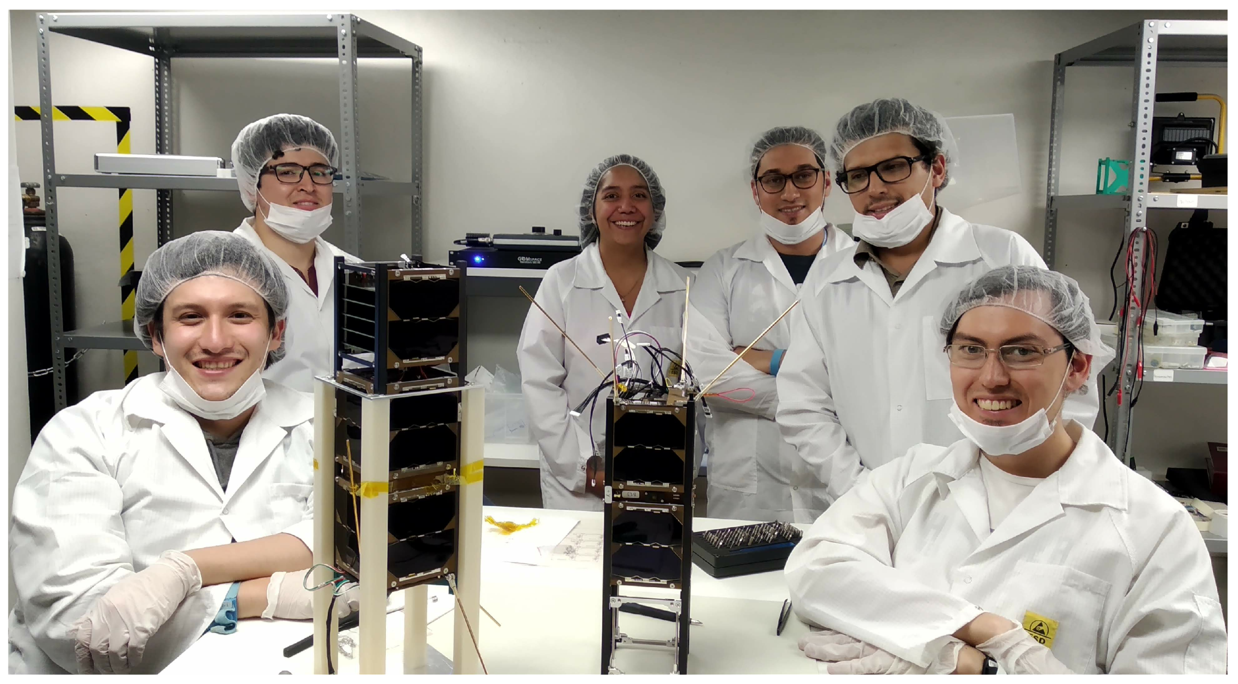
In the Space and Planetary Exploration Laboratory (SPEL) at the University of Chile, we are working on developing such types of missions, with a preliminary technology demonstration that will be carried in the following missions of the laboratory [9]. Preliminarily, we plan to deploy a femto-satellite version that contains a GPS to verify the position. This version will carry a magnetometer and a miniaturized particle counter that was tested in the SUCHAI-1 mission [10]. We will deploy the femto-satellite opportunistically to increase the sensing points in the ionosphere/magnetosphere. This increase in the sensing points allows us to study the dynamic evolution during a geomagnetic storm. An ionospheric/magnetospheric anomalous activity usually lasts for a couple of days [11]. This duration requires the femto-satellite to operate for a few days. The experiment will be with two 3U CubeSats, the SUCHAI-2 and SUCHAI-3 (Figure 1). We expect to launch them together in a similar orbit. SUCHAI-3 will serve as the mother-spacecraft of the femto-satellite, carrying and deploying it in some moment once in orbit. The femto-satellite will send the gathered data with a radio communication link to both CubeSats. In this research, we simulate a similar scenario to study the feasibility of using the radio links to estimate the location of a femto-satellite with only two CubeSats. This location estimation combines the Time Difference Of Arrival (TDOA) with the Angle Of Arrival (AOA) of the received signals.
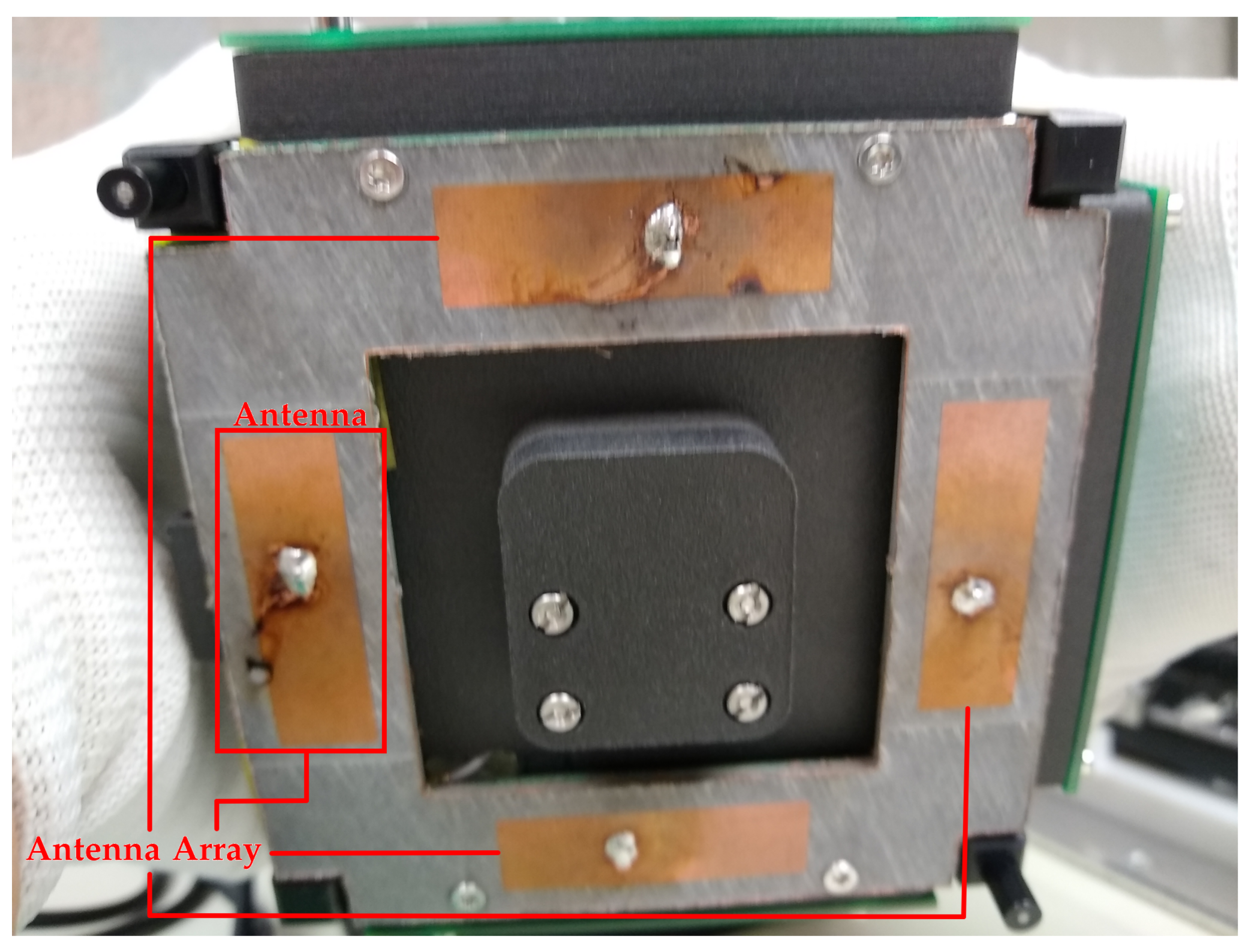
The TDOA method has been used for drone detection and localization [12], in storehouse environments [13], IoT [14] and by mobile users [15]. This method has also been used on larger satellites, using it to localize a satellite from the ground [16], as well as from other satellites in space [17]. The AOA method uses an antenna array to know the yaw (azimuth) and pitch (elevation) of the received signal. Placing the antennas in a square array [18] allows estimating both yaw and pitch instead of just one angle. A target can send a signal to multiple receivers with antenna arrays. The angles measured at the receivers with known locations provide the target position. This method has been used mostly on the ground for wireless sensor networks [19]. There is also research for the 5G cellular system, which uses antenna arrays in the stations, suggesting the possibility of locating a phone using the AOA with multiple transmission-reception points [20]. A work even suggested using two satellites to passively locate an object on the surface of the Earth using TDOA, Frequency Difference Of Arrival (FDOA), and AOA measurements [21]. Figure 2 shows our implementation of an antenna array.
We based our work on Yin et al. [22] localization method. Yin et al. estimated the location of a source using two stations in fixed and well-known positions. Our work studies the accuracy of this method when the stations are moving and have uncertainty in their positions. We study the performance of this method in the context of space. In this context, the stations are now CubeSats separated by 30 km and moving in a polar orbit. The position of these CubeSats is changing but is also affected by the accuracy of the on-board GNSS receivers. The source is a femto-satellite deployed from one of the CubeSats at a certain speed and direction (which we will determine in the next sections). We evaluate if different positions and directions of deployment change the performance of the localization method. The simulation of the deployment direction considers that the Attitude Determination and Control System (ADCS) is not perfect. The CubeSats combine range-based (TDOA) and angle-based (AOA) localization methods to estimate the femto-satellite position through the communication link. Each CubeSat is assumed to carry an antenna array, an ADCS, and a GNSS receiver. In our study, the femto-satellite transmits a beacon to the CubeSats, and the CubeSats then measure the beacon TDOA and AOA using antenna arrays. These CubeSats relay this information to the ground station, which combines it to estimate the femto-satellite position. We study the effect on the Cramér–Rao Bound (CRB) and the Root-Mean-Square Error (RMSE) of the femto-satellite location for different deployment directions, CubeSats location, and attitude determination and control precision. To evaluate the location precision, we developed a simulation tool that emulates the orbit of the satellites using the SGP4 model [23]. This simulation tool was developed in python and made available to the community as an open-source tool. It is hosted in the SPEL’s GitHub site at the following link: https://github.com/spel-uchile/Pypredict (last accessed on 15 December 2021).
2. Materials and Methods
The Two-Line Element set (TLE) consists of two 69-character lines of data provided by NORAD, that describe the orbit of a satellite. It includes orbital elements such as the inclination, the Right Ascension of the Ascending Node (RAAN), the eccentricity, the argument of the perigee, the mean anomaly, and the mean motion, which are necessary to determine a satellite’s position and velocity at a given time. For the simulations, we used as an example the TLE data of a 3U CubeSat from Planet Labs called FLOCK 4P-1 (Table 1) that is in LEO orbit. This CubeSat has an inclination of , a RAAN of , an eccentricity of , an argument of the perigee of , a mean anomaly of , and a mean motion of revolutions per day. We assumed that there are two CubeSats in the same orbit, one after the other. This is common for small CubeSat constellations since they are deployed from the same rocket. For this reason, we generated two CubeSats using the same TLE at two different time epochs, with a time-lapse of four seconds (around 30 km of separation). The CubeSat-1, or mother-CubeSat, is the one that deploys the femto-satellite and is behind the second CubeSat. The deployment considers a femto-satellite of 80 g and two CubeSats of 3.2 kg each. The simulation was made for an orbit of 17 November 2020, before the satellites arrive at the South Atlantic Anomaly. We propagated all the orbits using the SGP4 model [23].
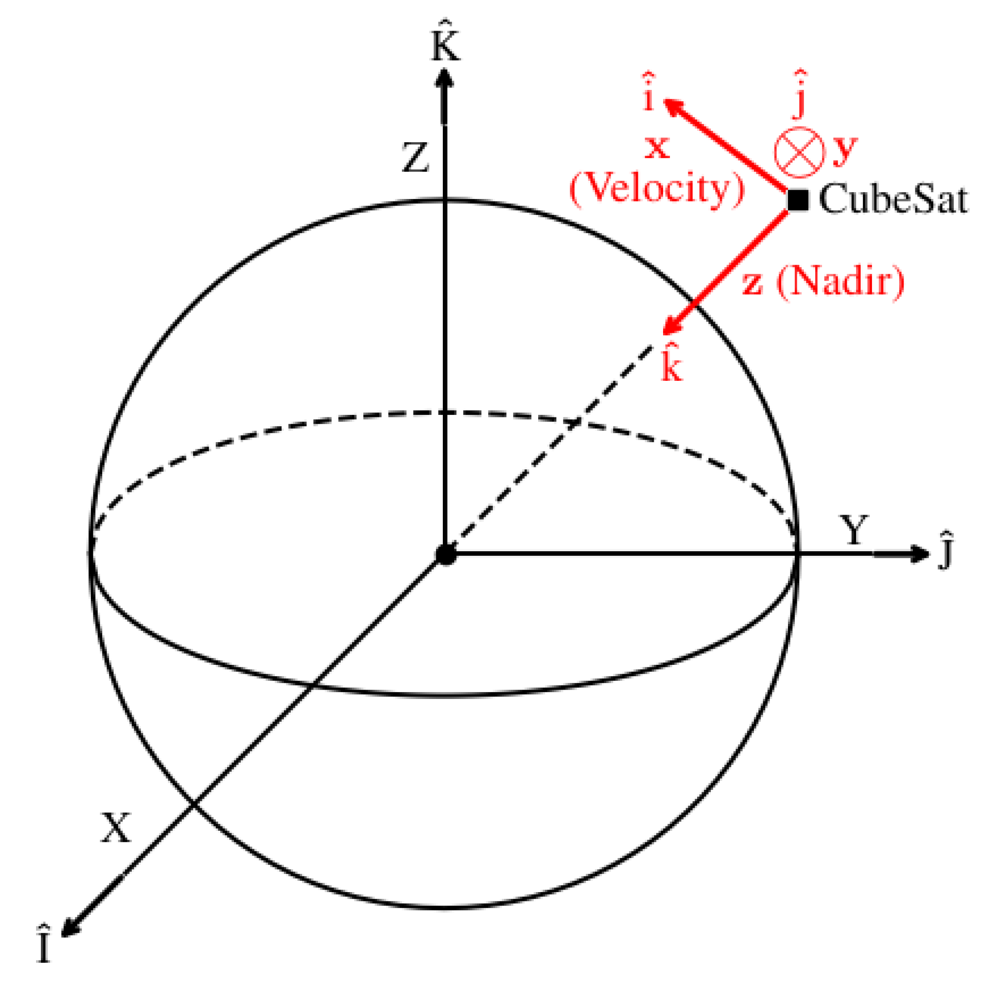
We use the Earth Centered Inertial (ECI) coordinate frame for the calculations of the satellite’s positions. The femto-satellite’s unknown position is represented by the vector while the CubeSats are at known positions , . The measurement of the CubeSat’s position is affected by the accuracy of their GNSS device, as seen in
where is a zero-mean Gaussian noise to model the accuracy of the GNSS device. The accuracy of each axis is equal to the overall accuracy divided by . We use the same measurement model as in [22] with one TDOA and two AOA pairs , but the elevation is because we are not limited to the ground. These angles correspond to each CubeSat’s Local Vertical/Local Horizontal (LVLH) frame, which is depicted in Figure 3.
There are five design parameters for this localization system: the deployment direction and speed, the point in the orbit where the deployment takes place, the accuracy of the attitude determination and control systems (ADCS), and the GNSS devices of the CubeSats. For this research, we will assume a speed of deployment of 1 m/s to focus on the rest of the design parameters.
We use the LVLH frame of the CubeSat with the Femto-satellite Orbital Deployer (FOD) to conduct the deployment simulations. Figure 3 illustrates the reference frame attached to the CubeSat. Different deployment directions and orbit’s point of deployment change the localization geometry. The geometry is directly related to the performance of the localization system. Due to the limitations of the ADCS, the femto-satellite’s deployment will not be in the desired direction with exactitude. The model of the deployment direction is
where and represent the yaw (azimuth) and pitch (elevation) of the deployment from the CubeSat’s LVLH frame, and are zero-mean Gaussian noises for the yaw and pitch. This is done to represent the accuracy of the attitude determination system (ADS) and the attitude control system (ACS), with a variance of . These values move the direction of deployment from the one intended, changing the localization geometry.
With the speed and direction of deployment, we calculate the new velocities for both the femto-satellite and the CubeSat that deploys it. We do this using the law of conservation of momentum. After obtaining the satellites’ position and velocity, we search for the TLE set that best describes these two vectors, starting from the original TLE file of the mother-CubeSat. For this purpose, we need to find the new inclination, RAAN, eccentricity, the argument of the perigee, mean anomaly, and mean motion. Since having six nested for loops takes too much time, we decided to select different groups of two to three orbital elements and search for the best fit iteratively. The ballistic coefficient, and the first and second derivatives of the mean motion, and , respectively, are set equal to the one provided by the TLE file. This approach does not impact the prediction accuracy for short-term orbit propagations as seen in [24].
The methodology for finding the best localization scenario is as follows. First, we simulate the deployment of the femto-satellite into different directions at 1 m/s. We compare them using the root Cramér–Rao Bound (CRB), which is statistically the lower limit of the error in the position estimation. We select the direction that yields the best results, and then we evaluate if there is any difference in which point of the mother-CubeSat’s orbit we deploy the femto-satellite. After selecting these values, we study how both the attitude determination and the attitude control systems’ accuracy affect the position estimation’s performance. We choose the accuracy of these systems based on the results and on the technology that is currently available. Similarly, we simulate GNSS devices with different accuracies for the CubeSats positions. With the results of the simulations, we choose the accuracy of a GNSS receiver based on what is on the market for space applications. Finally, we evaluate this localization system using the root CRB, the Root Mean Square Error (RMSE), and the estimation bias.
3. Results
When we simulate a deployment, we need to obtain the new Two-Line Element set (TLE) of both the mother-CubeSat and the femto-satellite. After searching for the TLE set that better fits the position and the new velocity for each of them, we found we had a distance error below 6 m and a speed error of less than 0.007 m/s between the theoretical one and the one provided by the new TLE set.
The simulations are three days after the deployment, for a time frame of 100 min. We advance the simulation three days since the mission operation proposes to deploy the femto-satellite after the beginning of a strong geomagnetic storm to study the magnetic variations at several points. The duration of the effects of the geomagnetic storm lasts a couple of days based on historical data [11]. We simulated a period of 100 min to guarantee the study of a complete orbit, which is around 94.5 min. We also wanted to calculate the performance for the worst-case scenario. There is a reduction in performance as the satellites separate over time. That is why we also evaluate at the end of three days.
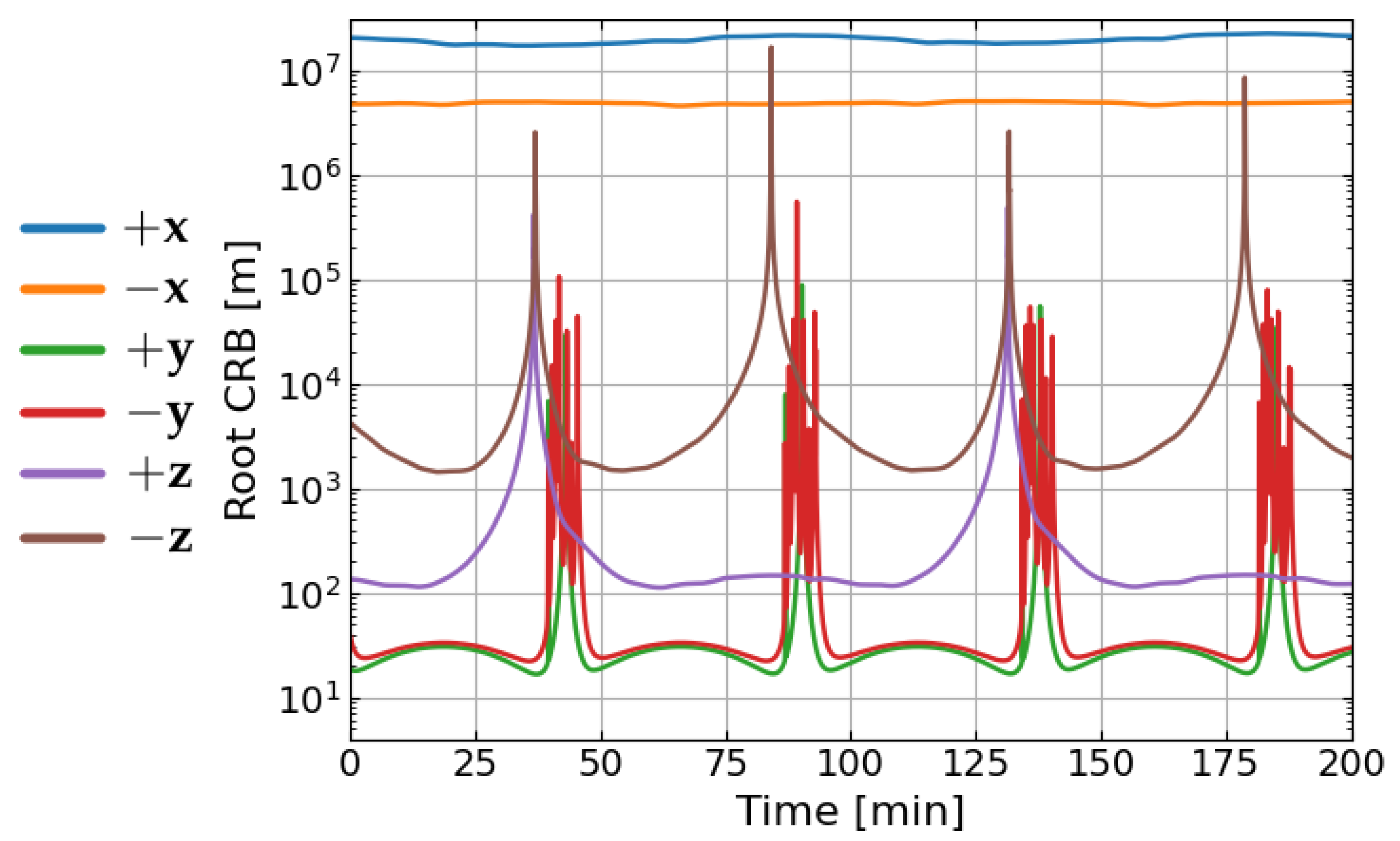
We searched for the best localization scenario, assuming an ADCS with perfect accuracy. For this purpose, we simulated the deployment in the positive and negative direction of the three axes of the mother-CubeSat’s LVLH frame. The x axis is in the direction of movement, the z axis points at the nadir, and the y axis is orthogonal to them. We selected ten orbit positions to deploy the femto-satellite, with a time step of ten minutes since the apogee. Then, we calculated the average of the root CRB for these ten scenarios. For the root CRB, we used the square root of the trace of the MSE matrix [22]. The root CRB indicates the best possible accuracy of the position estimator.
Figure 4 shows the root CRB for the six directions. The worst scenario is when the femto-satellite is launched on the x axis because it aligns with both CubeSats. The AOA method’s performance decreases when there is an alignment between the target and the receivers. We obtained the best results when the deployment was made in the y axis because the geometry is closer to the optimal for the AOA [25]. The positive direction has lower peaks than the negative one, so we chose that one.
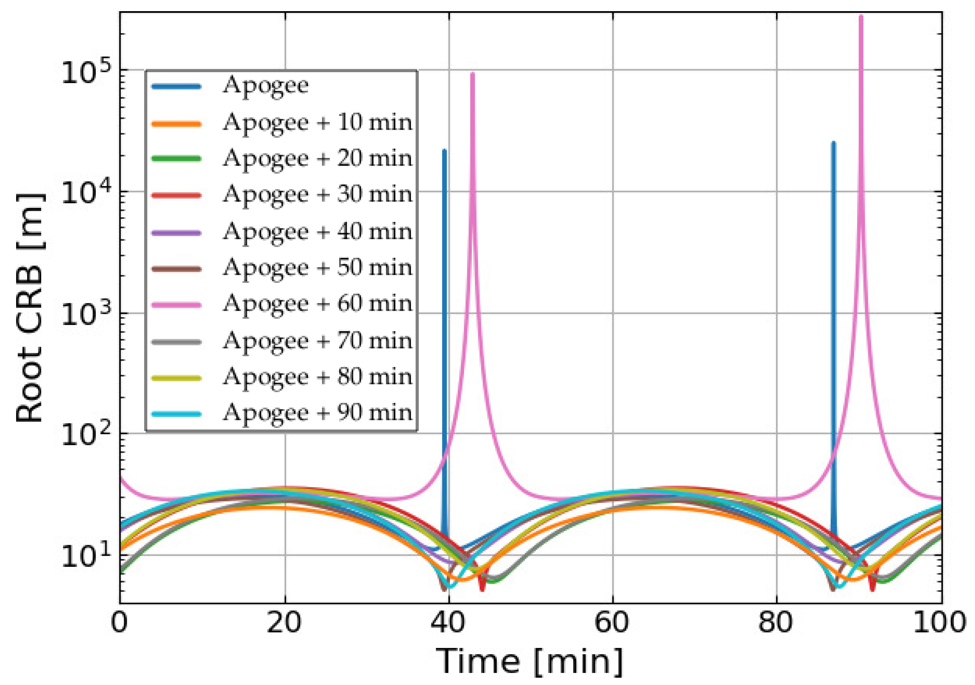
Now that we have chosen the deployment speed and direction, we need to find the orbit’s point to deploy the femto-satellite. Figure 5 shows different deployment points in the same orbit towards the positive y axis. Highly elliptical orbits, like Molniya, are more affected by this parameter than this simulated orbit. Still, there are some variations between cases. The lowest average root CRB occurs when the deployment is 10 min after the apogee.
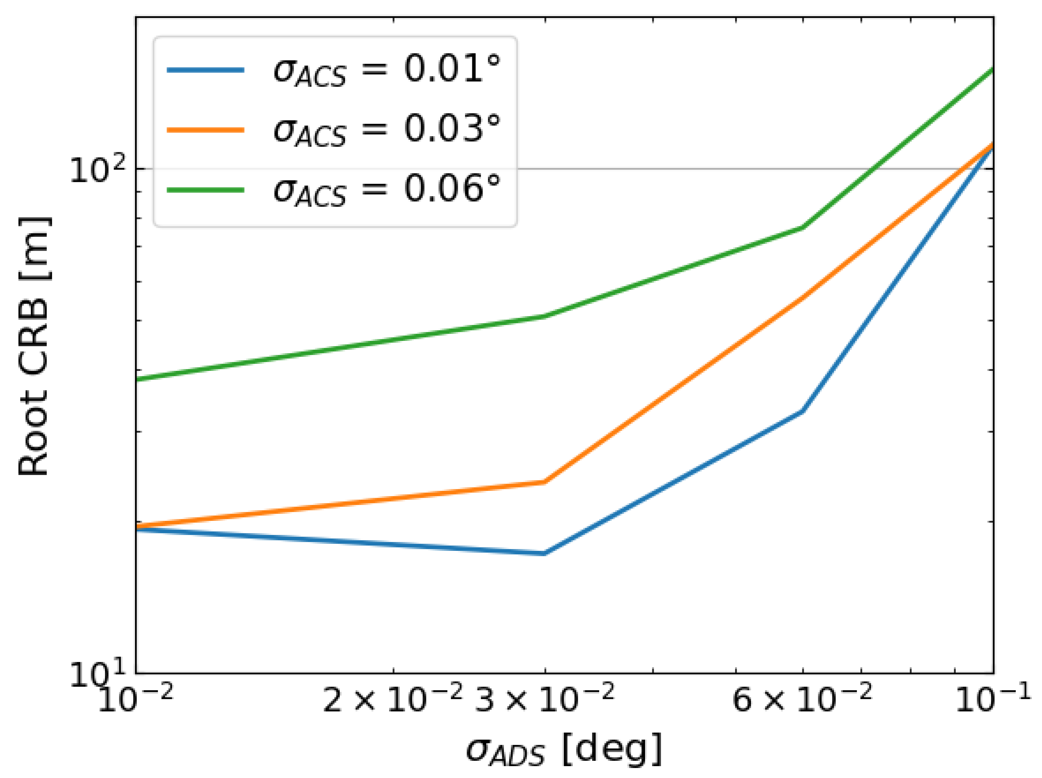
After selecting the orbit’s point for the deployment, we studied the impact of different attitude control and attitude determination systems on the root CRB. Figure 6 shows the root CRB of the localization system as both and increase. The curves are from three days after the deployment to see the effect on the performance. The root CRB is over 100 m for values of greater than . The difference between having an attitude control system, such as reaction wheels or magnetorquers, with an accuracy of or is around 20 m in the root CRB value. This information is useful to decide which devices are worth investing in according to the mission.
For the next figures, we display the root-mean-square error and the estimation bias given by Equations (3) and (4)
where is the ensemble’s position estimate, is the number of ensemble runs and is the number of deployment scenarios. In both the RMSE and the estimation bias, we calculate the average of deployments because we are simulating an ADCS without perfect accuracy. For all the simulations, we set and m, where is the standard deviation of the AOA method, and is the standard deviation of the TDOA method multiplied by the speed of propagation of the radio waves to transform it into a range difference. We also chose which is equal to 36 arcseconds of accuracy and can be obtained with a low-cost star tracker [26]. For the ACS, we used because Figure 6 shows that below this value, the root CRB decreases by around 20 m.
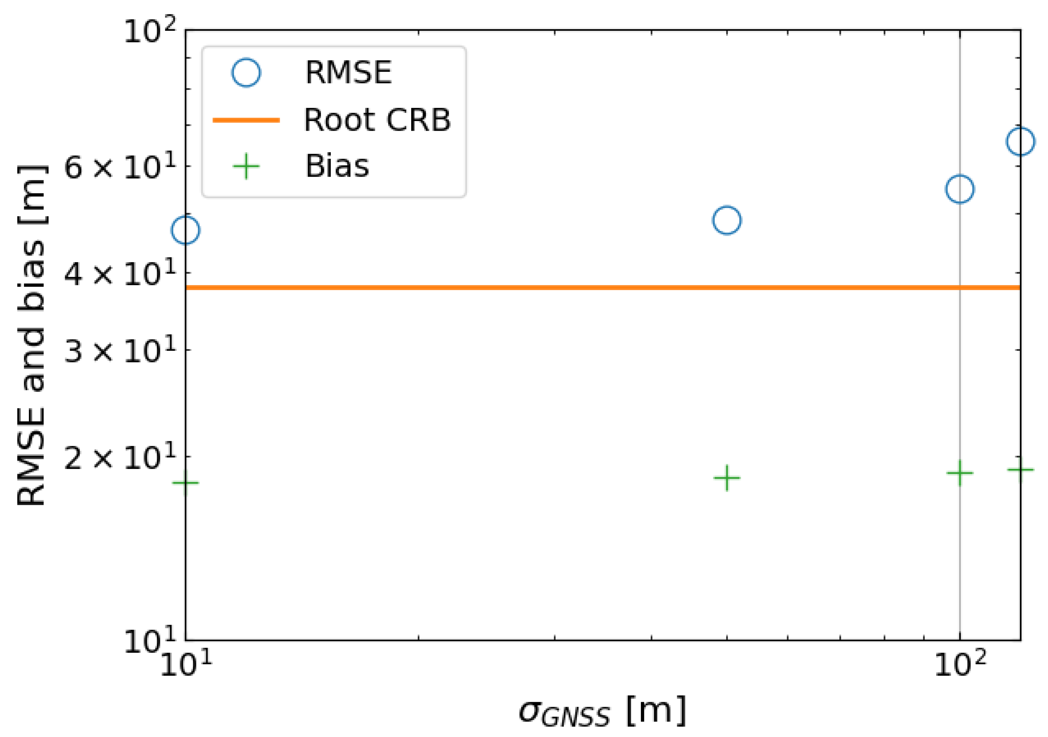
The accuracy of the GNSS devices on board the CubeSats also affects the performance of the localization system. To study the consequences, we simulated 5000 deployments towards the positive y axis. Then, we evaluated the localization system three days after deployment. For each deployment, we generated 5000 zero-mean Gaussian noises with a ranging from 10 m to 120 m. Figure 7 shows that the RMSE does not change until the accuracy of the GNSS is 50 m.
For the final simulation, we set m, since there are GNSS devices with that level of accuracy for CubeSats on the market, like the NewSpace Systems (NSS) GPS Receiver from CubeSat Shop. Figure 8 shows that the root CRB is below 30 m for most of the orbit three days after deployment. The purple line depicts the distance between the femto-satellite and the CubeSat that launched it. This distance oscillates and increases over time. This behavior is usual for deployments because, instead of just having a relative speed equal to the deployment speed, what happens is that the orbital parameters change. This change means that the femto-satellite and the CubeSats are now in different orbits. The red line shows the distance between the femto-satellite and the second CubeSat in kilometers. There is no noticeable change in this distance, but this could be related to the scale (kilometers instead of meters like the other curves) and the short time span. These variations may explain the saw-tooth shape of the bias that does not correlate perfectly with the parabolic shape of the angle nor with the distance between the femto-satellite and the mother-CubeSat.
We called the angle formed by the femto-satellite with the two CubeSats. When this angle is near , it means that the femto-satellite is between the CubeSats, and when it is near , it means that the mother-CubeSat is between the femto-satellite and the second CubeSat. In the simulations, we calculated the mean of , the case with the maximum , and the case with the minimum . There are cases with angles near or near because the deployment simulation considers the accuracy of the ADCS. Sometimes the femto-satellite is launched towards the positive axis deviated forward, and sometimes, it is deviated backward. If we also consider the oscillation of the distance between the femto-satellite and the mother-CubeSat, it is clear why the angle reaches these values. Figure 8 shows that these alignments coincide with the peaks of the root CRB where the estimation error increases. This increase occurs because these localization geometries are detrimental for the AOA method [27,28]. We obtained the best results when the angle is between and .
4. Discussion and Conclusions
This work presents the adaptation of a method that allows us to geolocalize a source with only two stations in low earth orbit (LEO). We based our work on a methodology intended originally for fix stations located on the ground [22]. Our geo-localization method also relies on the radio link between the source and the stations and on a system to combine the time difference of arrival (TDOA) and the angle of arrival (AOA) methods. We evaluated the geo-localization accuracy of this method for several LEO scenarios. The simulated scenarios used two 3U CubeSats (stations) and one femto-satellite (source), which is assumed to be deployed by one of these CubeSats. In contrast to the work by Yin et al. [22], our work allows the sources to go below of elevation of the receiving stations due to the absence of ground and adds the complexity of having moving stations (the two CubeSats). Additionally, we studied the impact that different uncertainties in the location estimation of these CubeSats have on the source location estimation. We simulated the deployment of the femto-satellite from the CubeSat and studied the impact on the source location accuracy for different deployment directions and accuracy levels of the on-board attitude determination and control systems for CubeSats.
We found in our analysis that with the current technology available for CubeSats, there are operational strategies that allow localization of the femto-satellite with an accuracy as good as 30 m, ∼80% of the time per orbit. We accomplished this by using only two CubeSats as receiving stations, without the necessity of using GNSS receivers on the source satellite. We will test this in space with the SUCHAI-2 and SUCHAI-3 missions [9] developed by the Space and Planetary Exploration Laboratory (SPEL) at the University of Chile (see Figure 1 and Figure 2). For the analysis, we developed a simulation tool available on the GitHub of the SPEL: https://github.com/spel-uchile/Pypredict (last accessed on 15 December 2021).
When one CubeSat is following another one, the simulations show that the performance is highly dependent on the direction of deployment (see Figure 4). The best scenario is when we deploy the femto-satellite towards the axis, perpendicular to the nadir and the direction of movement of the mother-CubeSat (see the red and green curves in Figure 4).
After choosing the direction of deployment, we studied the impact on the accuracy of the source location estimation depending on the point of the orbit where the deployment takes place. We found that these variations were negligible compared to the variations provoked by the deployment direction. Nevertheless, we obtain the lowest root CRB on average when deployment occurs 10 min after the apogee.
Since the accuracy of the source location estimation is highly dependent on the deployment direction, we analyzed the current attitude and control system technology in their capacity to ensure that the geometry formed by the CubeSats with the femto-satellite is as close to the optimal as possible. By using the reported accuracy of an open-source star tracker [26], we simulated the localization procedure for different accuracies of the attitude determination systems and the attitude control systems, where the lowest simulated values were and . Figure 6 shows that improving the accuracy of the used attitude determination and control systems improves the accuracy of the location estimation. However, the relation is not linear. For instance, the location estimation accuracy obtained with [, ] is the same than that reached with [, ], and the difference in the location estimation accuracy when using [, ] is a few meters less than the accuracy achieved when using [, ]. It tells us that for certain attitude control accuracy, there is a point where improving the attitude determination accuracy has a negligible impact on the accuracy of source location estimation.
Then, by using and , we studied how the accuracy of the on-board GNSS receivers affected the performance of the localization system. The simulations show that when the accuracy of the GNSS receivers is better than 50 m, the RMSE remains more or less constant (see Figure 7). Since several GNSS receivers offer m of accuracy, we selected this value.
After selecting the deployment direction and the ADCS and GNSS accuracies, we ran a final simulation to evaluate the localization accuracy achievable with the TDOA-AOA method. This system achieved a root CRB below 30 m and an RMSE near this value for most of the orbit. The only exception is when the three satellites align with each other. These alignments between the satellites generate geometries detrimental to the AOA method. Having a third CubeSat not aligned with the rest of the satellites allows the Time Difference Of Arrival (TDOA) method to solve this issue. However, we wanted to know if we could estimate the location using only two CubeSats, not only because the number of stations is lower but also because we have only two CubeSats in our mission [9]. These results show the feasibility of performing the remote geo-location of femto-satellites by using a communication link with patch antenna arrays to estimate the AOA, while estimating the TDOA of the signal using a GNSS clock signal. This approach will be tested in space by the SUCHAI-2 and -3 mission. The SUCHAI-3 will carry and deploy two femto-satellites once in space. The femto-satellites will carry PNI magnetometers for magnetospheric studies [5,7] and single-frequency GPS receivers to contrast the results of the method presented in this work. This approach, which includes the method and the deployment strategy, might be relevant to reduce the size, cost, and power consumption of femto-satellites while maintaining accuracy in their location estimation.
This method could also be useful for missions at very low altitudes (below 350 km) or missions developed for other celestial bodies. In addition, this technique might help estimate the orbits of other satellites in LEO (satellite tracking) by using a small number of CubeSats. The accuracy of the geo-location method might be improved, especially in this 20% of the orbit where the satellites are aligned, by taking advantage of the a priori knowledge that the source follows an orbital trajectory.
Author Contributions
Conceptualization, M.G.V.-V. and M.A.D.; methodology, M.G.V.-V. and M.A.D.; software, M.G.V.-V.; validation, M.G.V.-V.; formal analysis, M.G.V.-V.; investigation, M.G.V.-V.; resources, M.G.V.-V. and M.A.D.; data curation, M.G.V.-V.; writing—original draft preparation, M.G.V.-V. and M.A.D.; writing—review and editing, M.G.V.-V. and M.A.D.; visualization, M.G.V.-V.; supervision, M.G.V.-V. and M.A.D.; project administration, M.G.V.-V. and M.A.D.; funding acquisition, M.A.D. All authors have read and agreed to the published version of the manuscript.
Funding
This research was funded by the Air Force Office of Scientific Research (AFOSR) under award number FA9550-18-1-0249. This work has been also partially funded by the grants: CONICYT PIA ACT1405, FONDECYT Regular 1151476, FONDECYT Regular 1211144, FONDECYT Regular 1211695, FONDECYT Regular 1221907, QUIMAL 190004 and CONICYT-PFCHA/Doctorado Nacional/2017-21171111.
Institutional Review Board Statement
Not applicable.
Informed Consent Statement
Not applicable.
Data Availability Statement
The figures and simulations can be reproduced using the Python script called AOAwithTDOA.py, which is available in the GitHub webpage https://github.com/spel-uchile/Pypredict, last accessed on 15 December 2021.
Acknowledgments
We want to acknowledge Samuel T. Gutiérrez and Elías A. Obreque from SPEL for helping with the reviewing of this article.
Conflicts of Interest
The authors declare no conflict of interest. The funders had no role in the design of the study; in the collection, analyses, or interpretation of data; in the writing of the manuscript; or in the decision to publish the results.
References
- Belli, A.; Exertier, P. Long-term behavior of the DORIS oscillator under radiation: The Jason-2 case. IEEE Trans. Ultrason. Ferroelectr. Freq. Control 2018, 65, 1965–1976. [Google Scholar] [CrossRef] [PubMed]
- Manchester, Z.; Peck, M.; Filo, A. Kicksat: A Crowd-Funded Mission to Demonstrate the World’s Smallest Spacecraft. Small Satellite Conference. 2013. Paper SSC13-IX-5. Available online: https://digitalcommons.usu.edu/smallsat/2013/all2013/111/ (accessed on 6 January 2022).
- Hadaegh, F.Y.; Chung, S.J.; Manohara, H.M. On Development of 100-Gram-Class Spacecraft for Swarm Applications. IEEE Syst. J. 2016, 10, 673–684. [Google Scholar] [CrossRef] [Green Version]
- Barnhart, D.; Vladimirova, T.; Sweeting, M.; Balthazor, R.; Enloe, L.; Krause, H.; Lawrence, T.; McHarg, M.; Lyke, J.; White, J. Enabling Space Sensor Networks with PCBSat. Small Satellite Conference, Logan, UT, USA. 2007. Paper SSC07-IV-4. Available online: https://digitalcommons.usu.edu/smallsat/2007/all2007/30/ (accessed on 6 January 2022).
- Parham, J.B.; Kromis, M.; Einhorn, D.; Teng, P.; Posnov, S.; Levin, H.; Van Dessel, O.; Zosuls, A.; Walsh, B.; Semeter, J. Networked Small Satellite Magnetometers for Auroral Plasma Science. J. Small Satell. 2019, 8, 801–814. [Google Scholar]
- Yang, L.; Guo, J.; Fan, C.; Song, X.; Wu, S.; Zhao, Y. The design and experiment of stardust femto-satellite. Acta Astronaut. 2020, 174, 72–81. [Google Scholar] [CrossRef]
- Regoli, L.H.; Moldwin, M.B.; Pellioni, M.; Bronner, B.; Hite, K.; Sheinker, A.; Ponder, B.M. Investigation of a low-cost magneto-inductive magnetometer for space science applications. Geosci. Instrum. Methods Data Syst. 2018, 7, 129–142. [Google Scholar] [CrossRef] [Green Version]
- Perez, T.R.; Subbarao, K. A Survey of Current Femto-Satellite Designs, Technologies, and Mission Concepts. J. Small Satell. 2016, 5, 467–482. [Google Scholar]
- Diaz, M.; Zagal, J.; Falcon, C.; Stepanova, M.; Valdivia, J.; Martinez-Ledesma, M.; Diaz-Pena, J.; Jaramillo, F.; Romanova, N.; Pacheco, E.; et al. New opportunities offered by Cubesats for space research in Latin America: The SUCHAI project case. Adv. Space Res. 2016, 58, 2134–2147. [Google Scholar] [CrossRef]
- Gonzalez, C.; Rojas, C.; Becerra, A.; Rojas, J.; Opazo, T.; Diaz, M. Lessons learned from building the first chilean nano-satellite: The SUCHAI project. AIAA/USU Small Satellite Conference. 2018, pp. 1–9, Paper SSC18-WKX-08. Available online: https://digitalcommons.usu.edu/smallsat/2018/all2018/483/ (accessed on 6 January 2022).
- Haines, C.; Owens, M.; Barnard, L.; Lockwood, M.; Ruffenach, A. The variation of geomagnetic storm duration with intensity. Sol. Phys. 2019, 294, 1–15. [Google Scholar] [CrossRef] [Green Version]
- Mototolea, D.; Stolk, C. Detection and localization of small drones using commercial off-the-shelf fpga based software defined radio systems. In Proceedings of the 2018 International Conference on Communications (COMM), Bucharest, Romania, 14–16 June 2018; pp. 465–470. [Google Scholar]
- Yamasaki, R.; Ogino, A.; Tamaki, T.; Uta, T.; Matsuzawa, N.; Kato, T. TDOA location system for IEEE 802.11 b WLAN. In Proceedings of the IEEE Wireless Communications and Networking Conference, New Orleans, LA, USA, 13–17 March 2005; Volume 4, pp. 2338–2343. [Google Scholar]
- Chen, J.; Shi, T.; Liu, Y.; Wu, S. A Time-compensation TDOA-based Wireless Positioning Method for Multi-level IoT Positioning. In Proceedings of the 2019 15th International Wireless Communications & Mobile Computing Conference (IWCMC), Tangier, Morocco, 24–28 June 2019; pp. 1731–1736. [Google Scholar]
- Li, W.; Tang, Q.; Huang, C.; Ren, C.; Li, Y. A new close form location algorithm with AOA and TDOA for mobile user. Wirel. Pers. Commun. 2017, 97, 3061–3080. [Google Scholar] [CrossRef]
- Kaliuzhnyi, M.; Bushuev, F.; Shulga, O.; Sybiryakova, Y.; Shakun, L.; Bezrukovs, V.; Moskalenko, S.; Kulishenko, V.; Malynovskyi, Y. International network of passive correlation ranging for orbit determination of a geostationary satellite. Odessa Astron. Publ. 2016, 29, 203–206. [Google Scholar] [CrossRef] [Green Version]
- Shuster, S.; Sinclair, A.J.; Lovell, T.A. Initial relative-orbit determination using heterogeneous TDOA. In Proceedings of the 2017 IEEE Aerospace Conference, Big Sky, MT, USA, 4–11 March 2017; pp. 1–7. [Google Scholar]
- Kułakowski, P.; Vales-Alonso, J.; Egea-López, E.; Ludwin, W.; García-Haro, J. Angle-of-arrival localization based on antenna arrays for wireless sensor networks. Comput. Electr. Eng. 2010, 36, 1181–1186. [Google Scholar] [CrossRef]
- Tomic, S.; Beko, M.; Dinis, R. 3-D Target Localization in Wireless Sensor Networks Using RSS and AoA Measurements. IEEE Trans. Veh. Technol. 2017, 66, 3197–3210. [Google Scholar] [CrossRef]
- Menta, E.Y.; Malm, N.; Jäntti, R.; Ruttik, K.; Costa, M.; Leppänen, K. On the performance of AoA–based localization in 5G ultra–dense networks. IEEE Access 2019, 7, 33870–33880. [Google Scholar] [CrossRef]
- Bin, Y.Z.; Lei, W.; Qun, C.P.; Nan, L.A. Passive satellite localization using TDOA/FDOA/AOA measurements. IEEE Conf. Anthol. 2013, 1–5. Available online: https://ieeexplore.ieee.org/abstract/document/6784815 (accessed on 6 January 2022). [CrossRef]
- Yin, J.; Wan, Q.; Yang, S.; Ho, K. A simple and accurate TDOA-AOA localization method using two stations. IEEE Signal Process. Lett. 2015, 23, 144–148. [Google Scholar] [CrossRef]
- Vallado, D.; Crawford, P.; Hujsak, R.; Kelso, T. Revisiting spacetrack report# 3. In Proceedings of the AIAA/AAS Astrodynamics Specialist Conference and Exhibit, Keystone, CO, USA, 21–24 August 2006; p. 6753. [Google Scholar] [CrossRef] [Green Version]
- Liu, X.; Yuan, B.; Meng, Z. Microsatellite Autonomous Orbit Propagation Method Based on SGP4 Model and GPS Data. In Proceedings of the 2018 IEEE CSAA Guidance, Navigation and Control Conference (CGNCC), Xiamen, China, 10–12 August 2018. [Google Scholar] [CrossRef]
- Xu, S.; Doğançay, K. Optimal sensor placement for 3-D angle-of-arrival target localization. IEEE Trans. Aerosp. Electron. Syst. 2017, 53, 1196–1211. [Google Scholar] [CrossRef]
- Gutiérrez, S.T.; Fuentes, C.I.; Díaz, M.A. Introducing SOST: An Ultra-Low-Cost Star Tracker Concept Based on a Raspberry Pi and Open-Source Astronomy Software. IEEE Access 2020, 8, 166320–166334. [Google Scholar] [CrossRef]
- Doğançay, K.; Hmam, H. Optimal angular sensor separation for AOA localization. Signal Process. 2008, 88, 1248–1260. [Google Scholar] [CrossRef]
- Bishop, A.N.; Fidan, B.; Doğançay, K.; Anderson, B.D.; Pathirana, P.N. Exploiting geometry for improved hybrid AOA/TDOA-based localization. Signal Process. 2008, 88, 1775–1791. [Google Scholar] [CrossRef]
Figure 1.
Images of the SUCHAI-2 and -3 CubeSats during the integration process together with part of the development team at the Space and Planetary Exploration Laboratory (SPEL). The launch of these CubeSats is scheduled for 2022. They will carry magnetometers and a communication system to receive the data from two femto-satellites. Each of these femto-satellites will also carry a magnetometer. The femto-satellites will be carried and deployed by the SUCHAI-3 CubeSat. We are studying the feasibility of estimating the location of a radio source (femto-satellite) in a concrete scenario, in low earth orbit where there are only two CubeSats available to estimate the location of two femto-satellites in a future mission.

Figure 2.
We are currently developing an antenna array able to fit in one face of a CubeSat. This figure shows a four-antenna array located at the bottom of the satellite, near the deployment switches. Another antenna array will be on the side of the CubeSat. We will deploy the femto-satellites through the hole of one of the antenna arrays.

Figure 3.
The Earth-Centered Inertial (ECI) coordinate frame, in black, is used to calculate all the satellites’ positions, while the CubeSat’s Local Vertical/Local Horizontal (LVLH) frame, in red, is used for the deployment simulation. The x axis points towards the direction of movement, z to the nadir, and y is orthogonal to them.

Figure 4.
The root CRB indicates the best possible accuracy of the position estimator, and we used it to compare the six deployment directions. This figure shows the root CRB after three days since the deployment of the femto-satellite at 1 m/s. The orbit’s period is around 94.5 min. Each of the lines represents one of the six directions of deployment using the mother-CubeSat’s LVLH frame, and it is the average of 10 different deployment points of the orbit.

Figure 5.
Root CRB for deployments towards the positive y axis, at different points of the orbit. The points are separated by a time-lapse of ten minutes, starting at the apogee.
Figure 5.
Root CRB for deployments towards the positive y axis, at different points of the orbit. The points are separated by a time-lapse of ten minutes, starting at the apogee.

Figure 6.
Root CRB for different values of and . These values are related to the accuracy of the deployment system, so we study the effect on the performance of the localization system three days after deployment.
Figure 6.
Root CRB for different values of and . These values are related to the accuracy of the deployment system, so we study the effect on the performance of the localization system three days after deployment.

Figure 7.
Source localization RMSE and bias as increases from 10 m to 120 m, at three days after the deployment.
Figure 7.
Source localization RMSE and bias as increases from 10 m to 120 m, at three days after the deployment.

Figure 8.
Source localization RMSE and bias for the first 100 min after deployment. The line is the distance between the femto-satellite and the mother-CubeSat, displayed in meters. The line is the distance in kilometers between the femto-satellite and the second CubeSat. The line represents the angle between the vector femto-satellite-CubeSat-1 and femto-satellite-CubeSat-2.


Table 1.
This is the Two-Line Element set (TLE) of the FLOCK 4P-1 that we used to simulate two 3U CubeSats. To separate the CubeSats, we used an epoch difference of four seconds, equivalent to around 30 km of distance.
Table 1.
This is the Two-Line Element set (TLE) of the FLOCK 4P-1 that we used to simulate two 3U CubeSats. To separate the CubeSats, we used an epoch difference of four seconds, equivalent to around 30 km of distance.
| 1 44814U 19081L 20321.73053029 .00001305 00000-0 63025-4 0 9996 |
| 2 44814 97.4788 21.6285 0013387 80.2501 280.0246 15.20374749 54001 |
Publisher’s Note: MDPI stays neutral with regard to jurisdictional claims in published maps and institutional affiliations. |
© 2022 by the authors. Licensee MDPI, Basel, Switzerland. This article is an open access article distributed under the terms and conditions of the Creative Commons Attribution (CC BY) license (https://creativecommons.org/licenses/by/4.0/).
Share and Cite
MDPI and ACS Style
Vidal-Valladares, M.G.; Díaz, M.A. A Femto-Satellite Localization Method Based on TDOA and AOA Using Two CubeSats. Remote Sens. 2022, 14, 1101. https://doi.org/10.3390/rs14051101
AMA Style
Vidal-Valladares MG, Díaz MA. A Femto-Satellite Localization Method Based on TDOA and AOA Using Two CubeSats. Remote Sensing. 2022; 14(5):1101. https://doi.org/10.3390/rs14051101
Chicago/Turabian StyleVidal-Valladares, Matías G., and Marcos A. Díaz. 2022. "A Femto-Satellite Localization Method Based on TDOA and AOA Using Two CubeSats" Remote Sensing 14, no. 5: 1101. https://doi.org/10.3390/rs14051101
Note that from the first issue of 2016, this journal uses article numbers instead of page numbers. See further details here.