
Physical and Biochemical Responses to Sequential Tropical Cyclones in the Arabian Sea
by
 , ,
, ,
Tongyu Wang
1,2 ,
,
Fajin Chen
2,
Shuwen Zhang
1,*,
Jiayi Pan
3,
Adam T. Devlin
3,
Hao Ning
2 and
Weiqiang Zeng
2 1
Institute of Marine Science, Shantou University, Shantou 515063, China
2
College of Ocean and Meteorology, Guangdong Ocean University, Zhanjiang 524088, China
3
School of Geography and Environment, Jiangxi Normal University, Nanchang 330022, China
*
Author to whom correspondence should be addressed.
Remote Sens. 2022, 14(3), 529; https://doi.org/10.3390/rs14030529
Submission received: 6 December 2021
/
Revised: 18 January 2022
/
Accepted: 19 January 2022
/
Published: 23 January 2022
(This article belongs to the Special Issue Remote Sensing of Coastal Waters, Land Use/Cover, Lakes, Rivers and Watersheds II)
Abstract
:The upper-ocean physical and biochemical responses to sequential tropical cyclones (TCs) Kyarr and Maha in the Arabian Sea (AS) were investigated using data from satellites and Bio-Argo floats. Corresponding to slow and strong sequential TCs, two cooling processes and two short chlorophyll a (chl-a) blooms occurred on the sea surface, separated by 6–7 days, and three cold eddies appeared near the TC paths, with sea surface temperatures dropping more than 6 °C. Phytoplankton blooms occurred near cold eddies e1, e2, and e3, with chl-a concentrations reaching 12.76, 23.09, and 16.51 mg/m3, respectively. The depth-integrated chl-a analysis confirmed that the first chl-a enhancement was related to the redistribution of chl-a associated with TC-induced Ekman pumping and vertical mixing at the base of the mixed layer post-TC Kyarr. The subsequent, more pronounced chl-a bloom occurred due to the net growth of phytoplankton, as nutrient-rich cold waters were brought into the euphotic layer through Ekman pumping, entrainment, and eddy pumping post-TC Maha. Upwelling (vertical mixing) was the dominant process allowing the resupply of nutrients near (on the right side of) the TC path. The results derived from a biogeochemistry model indicated that the chl-a evolution was consistent with the observations recorded on Bio-Argo floats. This study suggests that in sequential TC-induced phytoplankton blooms, the redistribution of chl-a is a major mechanism for the first bloom, when high chl-a concentrations occur in the subsurface layer, whereas the second bloom is fueled by nutrients supplied from the deep layer.
1. Introduction
Identifying the response of the upper ocean to tropical cyclones (TCs) is one of the most challenging problems in oceanography [1,2,3,4]. As a TC passes, the clockwise rotation of the wind stress on the right side of the cyclone resonates with the near-inertial oscillation in the Northern Hemisphere. This triggers strong surface divergence, upwelling, and entrainment [1,5], resulting in substantial sea surface cooling after the TC passage [6,7,8]. For example, Typhoon Kai-Tak, which occurred in 2000 in the South China Sea, caused a maximum sea surface cooling of 10.8 °C [9]. Thus, TCs play an essential role in temperature redistribution and air–sea heat flux exchanges in the upper ocean. Simultaneously, a decrease in the sea surface temperature (SST) also has a significant negative feedback effect on the TC intensity, weakening or possibly shutting down the energy supply to a TC [10,11,12,13].
At present, satellite remote sensing observations are a powerful data source for investigating the characteristics and mechanisms of ocean color element responses to TCs [14]. Extensive studies have been conducted on the physical and biogeochemical responses of the ocean to TCs based on satellite observations [14,15,16,17,18,19]. Remote-sensed chlorophyll a (chl-a) is widely used to produce higher resolution images of phytoplankton concentrations. Strong blooms of phytoplankton are occasionally detected when slow-moving TCs linger over a region [14,18]. Pan et al. [20] found that the chl-a blooms during a typhoon event may be attributed to multiple factors related to the ocean dynamic conditions and cyclone characteristics. However, due to the lack of in situ measurements during short-duration TC forcing, systematic investigations of the spatial and temporal structure of plankton evolution with TC wind forcing are still insufficient [21], and particularly investigations of biochemical and physical processes, and the role of wind forcing in biological reproduction [22,23]. Overwhelming evidence shows that the phytoplankton blooms that occur during TCs are related to phytoplankton growth and the redistribution of phytoplankton by physical processes [22,23]. A recent study by Wang et al. [23] suggested that TC-induced ocean mixing is a major mechanism for ocean surface cooling and phytoplankton blooms in a short period. Chai et al. [24] showed that typhoon-induced mixing dominated the variability of surface chl-a during the passage of Trami, leading to the redistribution of chl-a within the upper ocean. Entrainment mixing can transport nutrient-rich cold waters from the deep layer to the euphotic zone, sustaining elevated chl-a growth [21,25,26,27]. More importantly, in addition to transporting nutrients upward, the entrainment mixing induced by TCs can also carry phytoplankton in the euphotic layer to deeper layers, leading to a decrease in euphotic layer phytoplankton. Therefore, investigations of the relative roles of these different processes, including phytoplankton growth, nutrient supplies, and phytoplankton redistribution, are of great significance for understanding ecosystem dynamics influenced by TCs. Studying the vertical variations in the biochemical elements in the water column is one of the most important ways researchers can understand the reactive responses of ecosystems during a TC.
Although surface data, such as SST and chl-a data, are relatively easy to obtain by satellite altimetry methods, obtaining high-resolution in situ data (via moored arrays, gliders, or towed instruments) of the profile distributions of chl-a and nutrients during the passage of a TC is extremely difficult, especially from the subsurface layer. In addition, obvious regional differences exist in the temporal and spatial distributions of global Argo observation data, mainly reflected in the Bio-Argo observation data. For example, only a handful of Bio-Argo observation data are available in the South China Sea and the Northwest Pacific Ocean, whereas a large amount of Bio-Argo data representing the surrounding waters at the same latitudes (Arabian Sea: AS) provide a good opportunity to study the ecological response of the upper ocean to TCs. The AS in the western North Indian Ocean is a region where important air–sea interactions occur, and they are strongly influenced by the seasonally reversed Indian monsoon system. The monsoon system can induce substantial seasonal variations in upper-ocean circulation, SSTs, mesoscale eddies, and heat budgets [28,29]. In the western North Indian Ocean, TCs can form in the pre-summer monsoon (May–June) and post-summer monsoon (October–November) periods [30]. Annually, one or two TCs can be generated over the AS, and few of these cyclones become sufficiently intense to be classified as very severe or supercyclonic storms [31]. Kuttippurath et al. [32] demonstrated that the average chl-a concentration associated with TC-induced phytoplankton blooms is approximately 1.65 mg/m3, which is approximately 20–3000% higher than the average open ocean or pre-TC chl-a levels. As global warming develops, the number of extremely severe TCs is likely to increase in the AS, meaning that the upper ocean has a more intense response to TCs [33]. The chl-a concentrations associated with TC activities have been increasing steadily over the past 20–35 years; this increase is mainly attributed to the increasing intensities of strong TCs [34]. The increasing trend in primary production associated with TC activities can partially mitigate the declining trend of ocean productivity under the background of global warming. TC frequencies and TC-induced phytoplankton blooms are high in the post-summer monsoon period in the AS, and the strong winds associated with TCs initiate intense upwelling, resulting in the enhancement of surface nutrients after the passage of TCs [32].
In this study, we aimed to investigate the dominant phytoplankton biomass processes in response to two TCs and analyze the biophysical dynamics of the ocean based on satellite, Bio-Argo, and biogeochemistry model datasets. The vertical profiles of physical and biogeochemical parameters measured by six Bio-Argo floats, in addition to the biogeochemistry model datasets characterizing the temporal evolutions of chl-a and nitrate concentrations, were used to identify phytoplankton dynamics. We explored whether local phytoplankton growth resulted from the replenishment of nutrients or from subsurface phytoplankton redistribution by vertical transport during sequential TCs, Kyarr and Maha. This investigation may improve our understanding of ocean biophysical dynamics, which is of fundamental importance in global carbon cycles.
2. Materials and Methods
2.1. Remote Sensing Data
The daily merged satellite-derived chl-a concentration data product was obtained from observations from multisource satellite sensors (the Sea-viewing Wide Field-of-view Sensor (SeaWiFS (National Aeronautics and Space Administration: NASA)), Moderate-resolution Imaging Spectroradiometer (MODIS (NASA)), Medium-resolution Imaging Spectrometer (MERIS (European Space Agency: ESA)), Visible Infrared Imaging Radiometer Suite-Suomi National Polar-orbiting Partnership (VIIRS-SNPP (NASA)) and Joint Polar Satellite System (JPSS1(ESA)), and Ocean Land and Colour Instrument-Sentinel-3A and -3B (OLCI-S3A and S3B(ESA))); these products provide end-users with the best chl-a concentration estimates at a spatial resolution of 4 km. The dataset is available on the website of the Copernicus Marine Environmental Monitoring Center (CMEMS, http://marine.copernicus.eu/ (accessed on 1 April 2021)) and was used to characterize the biomass dynamics at the sea surface [35]. SST and 10 m wind field data were downloaded from the Remote Sensing Systems data center (RSS, http://www.remss.com/ (accessed on 1 April 2021)). The 10 m wind data were used to calculate the wind stress. The spatial resolutions were 9 km and 25 km for the SST and 10 m wind field data, respectively, and their temporal resolutions were 1 day and 6 h, respectively. Sea level anomaly (SLA) and geostrophic current data were obtained from the CMEMS with a spatial resolution of 25 km and a temporal resolution of 1 day. We also used daily multisource (SeaWiFS, MODIS, and MERIS) composite cloud-corrected photosynthetically available radiation (PAR) (I0: Einstein m−2d−1) data with an attenuation coefficient at a 490 nm wavelength (K490) and a 4 km resolution to retrieve the light conditions in the upper oceans [36]; these data were downloaded from the following website: http://hermes.acri.fr/ (accessed on 1 April 2021).
2.2. In Situ Observations
As a part of the India Argo project (ftp://ftp.ifremer.fr/ifremer/argo (accessed on 5 April 2021)), 14 Bio-Argo floats equipped with biogeochemical and conductivity temperature-depth (CTD) sensors were deployed in the AS to collect ocean data. In this study, high-quality in situ data, e.g., temperature, chl-a, and dissolved oxygen (DO) concentration data recorded by floats in the AS from 5 October to 30 November 2019 were used, focusing on the timings of TC Kyarr and TC Maha. The Bio-Argo float observations were performed at 5-day or 10-day intervals from depths of 5 m to 2000 m. Six floats, labeled 2902175, 2902205, 2902210, 2902202, 2902272, and 2902120, and located in high-chl-a patches were selected in this study (Figure 1). Furthermore, observations from floats 2902272 and 2902210 in cold eddies e1 and e2, respectively, were selected to reveal the changes in vertical physical and biochemical structures. The statistical results of these float data are listed in Table 1.
Multiyear average nitrate profiles extracted from the World Ocean Atlas 2018 (WOA18, https://www.nodc.noaa.gov/ocs/woa18 (accessed on 1 April 2021)) were also used to represent the oceanic nutrient levels in October in the upper ocean above 200 m.
2.3. Model Data
The Nucleus for European Modelling of the Ocean (NEMO) version of the Global-Analysis-Forecast-Bio-001-028 dataset (v3.6-Stable) was used in this study [37], and it is derived from the daily CMEMS (Global-Analysis-Forecast-Phy-001-024) product [38]. The initial nitrate, phosphate, silicate, and DO conditions were obtained from the World Ocean Atlas 2013 (https://www.nodc.noaa.gov/OC5/woa13/ (accessed on 1 April 2021)). The operational Mercator Ocean biogeochemical global ocean analysis and forecast system at 1/4 degrees was used to generate 3D global ocean forecasts with weekly updates. The time series is aggregated in time, in order to obtain a full two-year sliding window time series. These data products include daily and monthly mean profiles of biogeochemical parameters, such as chl-a, nitrate, phosphate, silicate, DO, dissolved iron, primary production, phytoplankton, pH, and surface partial pressure of carbon dioxide over the global ocean. The Global-Analysis-Forecast-Bio-001-028 product has a horizontal resolution of 25 km, with 50 vertical layers from a depth of 0 to 5700 m. The product is published on the CMEMS dissemination server after automatic and human quality controls, and is available online and disseminated through the CMEMS Information System. The quality information document for Global Biogeochemical Analysis and Forecast Product that compares the model and the ocean color observations shows that the statistics are very good in the open sea (depth higher than 1000 m). The model and float chl-a concentrations compare reasonably well, and have a correlation coefficient of 0.81, a positive bias of 0.26, and a RMSE of 0.59 [37].
2.4. Methods
2.4.1. Ekman Pumping Velocity
As Ekman transport is affected by wind stress and Coriolis forces in the horizontal direction, sea water converges and diverges, influencing the Ekman pumping velocity (EPV) [1]:
where and are the sea-water density and the Coriolis parameter, respectively, is the Coriolis force, is the rotational angular velocity of the Earth, is the latitude, is the density of ocean water, and is the wind stress. The wind stress is calculated as follows:
where is the density of air, is the wind speed 10 m above sea level, and is the drag coefficient [39]. The drag coefficient is calculated as follows:
2.4.2. Mixed Layer Depth and Euphotic Layer Depth
The mixed layer depth (MLD) was calculated from the Bio-Argo float temperature and salinity profiles using two criteria: a change in temperature of 0.2 °C relative to the value at a 10 m depth and a change in density of 0.02 kg/m3 relative to the value at a 10 m depth [40]. For each profile, the mean of these two values was chosen to indicate the MLD.
PAR is the spectral range of solar radiation from 400 to 700 nm that photosynthetic organisms are able to use in the process of photosynthesis. KD490 can be converted into the attenuation coefficient at PAR wavelengths (K) using the following equation [41]:
The euphotic layer depth, defined here as the depth at which 1% of surface irradiance penetrates, was estimated from I0 assuming the Lambert–Beer relationship:
2.4.3. Wind Work and Forcing Time
The vertical entrainment caused by TCs can disrupt water stratification and bring nutrients upward into the surface layer. During a TC, strong winds inject high kinetic energy into the ocean, and the work done by the wind stress () to the ocean surface can therefore be calculated as follows [4]:
where u and v are the ocean surface velocities and are the wind stress components in the x and y directions, respectively.
The translation speed of each TC was estimated based on the method outlined by Mei et al. [42]. The temporal resolution of the wind field data was interpolated to 0.5 h, the region with wind speeds higher than 17 m/s was identified as the TC-influenced region, and the cyclone wind forcing time was determined using the duration of the cyclone-influenced region [4].
3. Results
3.1. Sequential Tropical Cyclones and the Study Area
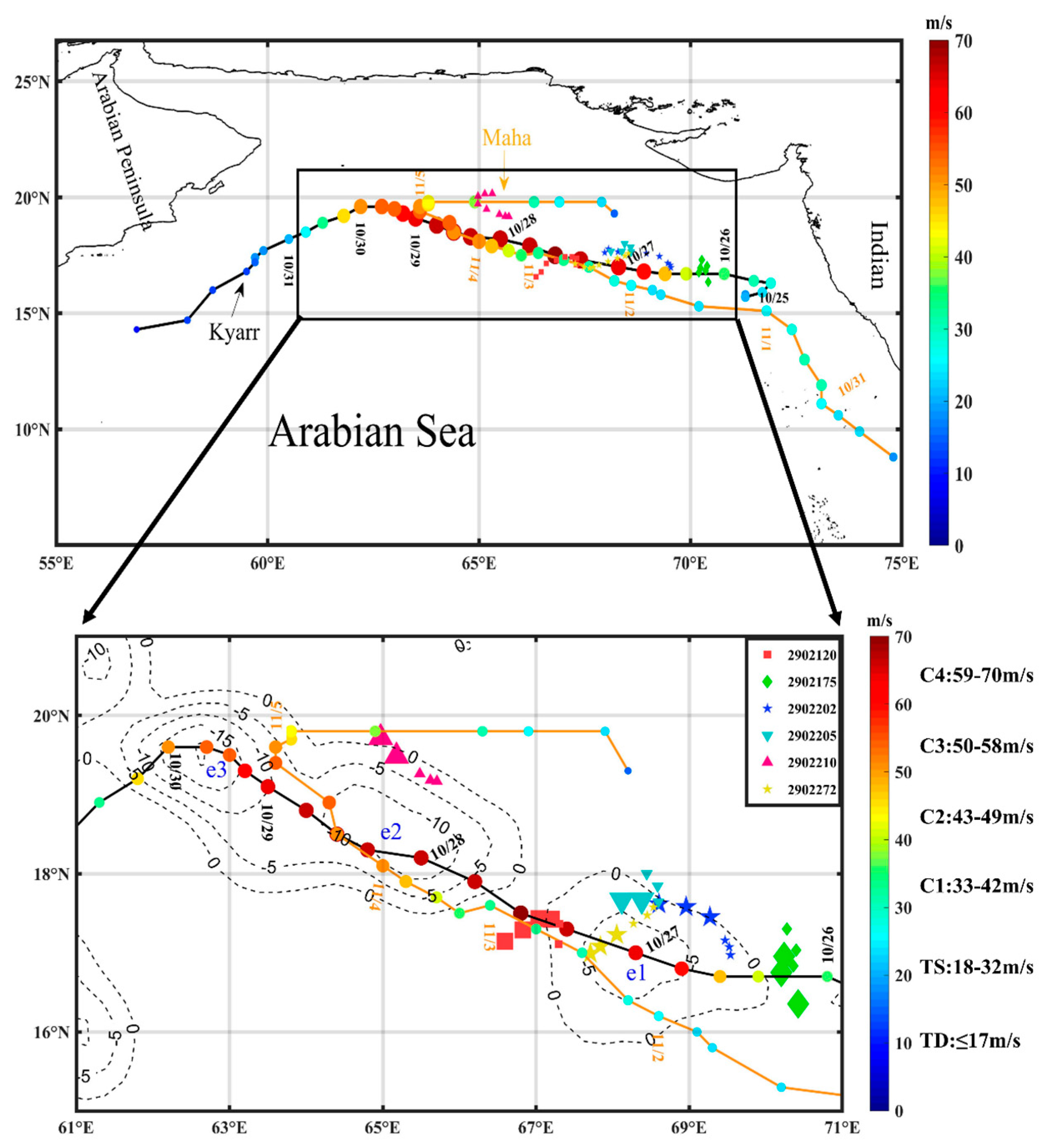
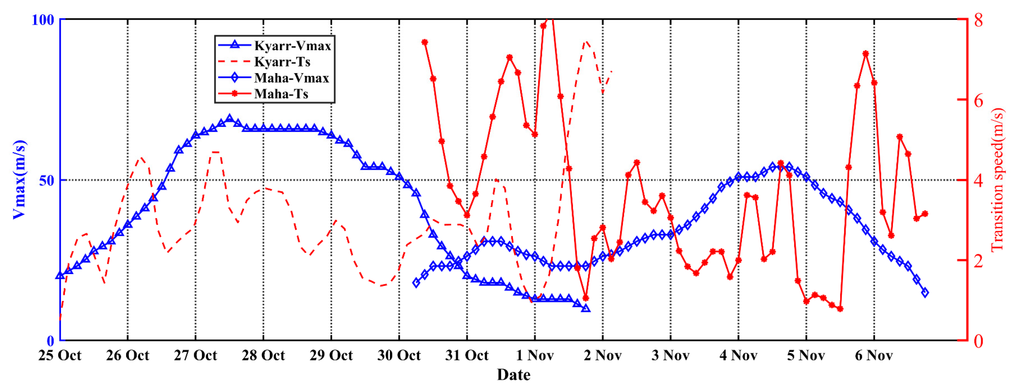
The best-track data representing the sequential TCs Kyarr and Maha were obtained from the International Best Track Archive for Climate Stewardship (IBTrACS; https://www.ncei.noaa.gov/ (accessed on 1 April 2021)) and included the maximum sustained wind speed at the sea surface and the TC center locations at 6 h intervals. The TC classification was based on the Saffir–Simpson hurricane scale (Figure 1). TCs Kyarr and Maha passed over the AS during the period from 25 October to 5 November 2019, and the two TCs moved northwestward in similar routes and reached the levels of Category 4 and Category 3 over the study area (61–71°E and 15–21°N), respectively. First, TC Kyarr was generated and reached the TC level at 15.8°N and 71.3°E and became a Category-1 TC at 00:00 on 26 October. It reached the Category-4 level at noon on 27 October with a maximum wind speed of 71 m/s and maintained this intensity and an average translation speed of 3.4 m/s until 29 October. The TC induced strong mixing and upwelling with cold subsurface waters due to the high winds associated with the slowly moving TC; these processes significantly lowered the SSTs, leading to energy losses into the ocean over a sufficiently long period of time to cause rapid decay [12]. Then, TC Kyarr began to weaken as it turned southwestward (Figure 2). Afterward, TC Maha formed at 8.8°N and 74.8°E and moved northwestward at 06:00 on 30 October; then, it intensified over the northwest AS and became a Category-3 TC with a maximum wind speed of 48 m/s and an average translation speed of 3.8 m/s on 4 November (Figure 1 and Figure 2). The time interval of the sequential TCs entering the study area was 5 days.
3.2. Horizontal Distributions of EPV, SST, SLA and Chl-a
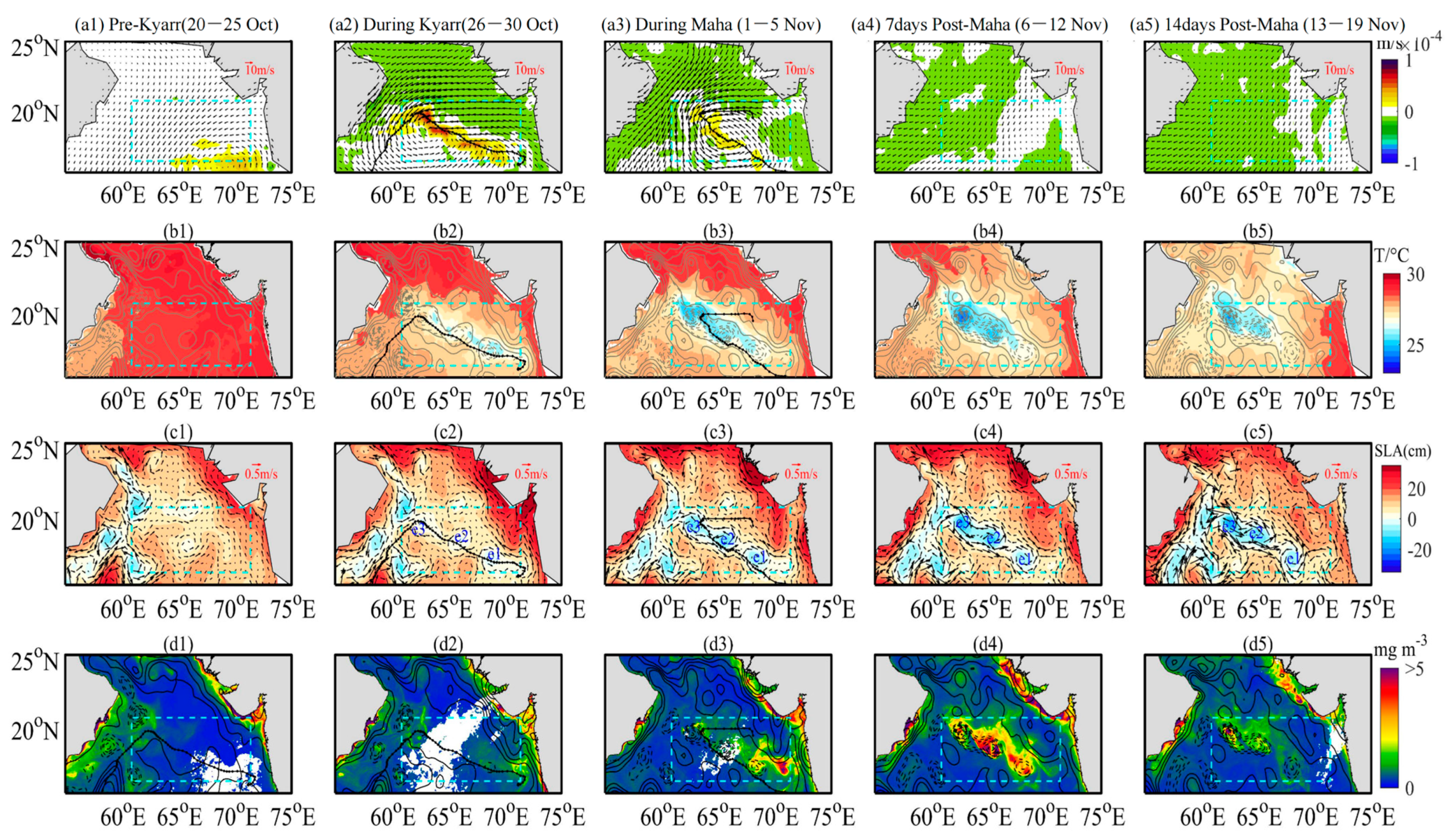
Prior to TCs Kyarr and Maha, the northeast monsoon prevailed over the study area (Figure 3(a1)), and the SSTs were warmer than 29 °C (Figure 3(b1)). As TC Kyarr entered the AS, cyclonic winds dominated over the study area (Figure 3(a2)). After TC Kyarr passed from 29 October to 5 November, the sea surface continued to cool, and the maximum temperature decrease was more than 5 °C (Figure 4b). At this time, three weak, cold centers can be seen on the sea surface along the track of TC Kyarr (Figure 3(b2)). After the passage of TC Maha, the SSTs continued to cool, and three cold patches expanded with maximum SST cooling magnitudes of approximately 6 °C (Figure 3(b3)); the expansion of these three cold patches was halted after 19 November (Figure 3(b5)). Sea surface cooling was not significantly enhanced along the path of TC Maha, probably because the system was moving over the ocean with a much deeper mixed layer [43]. After the passage of TC Kyarr, the three cold centers were related to three cold eddies e1, e2, and e3 with radii of 166.5, 175.2, and 186.4 km, respectively (Figure 3(c2)); the minimum SLAs of these three cold eddies were −7.26, −14.27, and −20.56 cm. The spatial patterns of the three eddies were consistent with the horizontal structure of the chl-a biomass patches (Figure 3(d4)). The maximum response values of chl-a in e1, e2, and e3 were 12.76, 23.09, and 16.51 mg/m3, respectively, from 20 October to 19 November 2019. As the two TCs moved slowly in e2 and e3, larger chl-a concentrations appeared in these eddies. The surface chl-a concentration increased by 31.6 times compared with that measured before the passage of the TCs. After the passage of TC Maha, the minimum SLAs of three cold eddies with radii of 166.5, 175.2, and 186.4 km (Figure 3(c2)) were −7.26, −14.27, and −20.56 cm, respectively. Cold eddy e2 and cold eddy e3 merged to become one cold eddy, and the e1 and e2 eddies strengthened (Figure 3(c4)); by 19 November, these cold eddies had strengthened (Figure 3(c5)), with maximum geostrophic swirl speeds of 0.46 and 0.69 m/s, respectively.
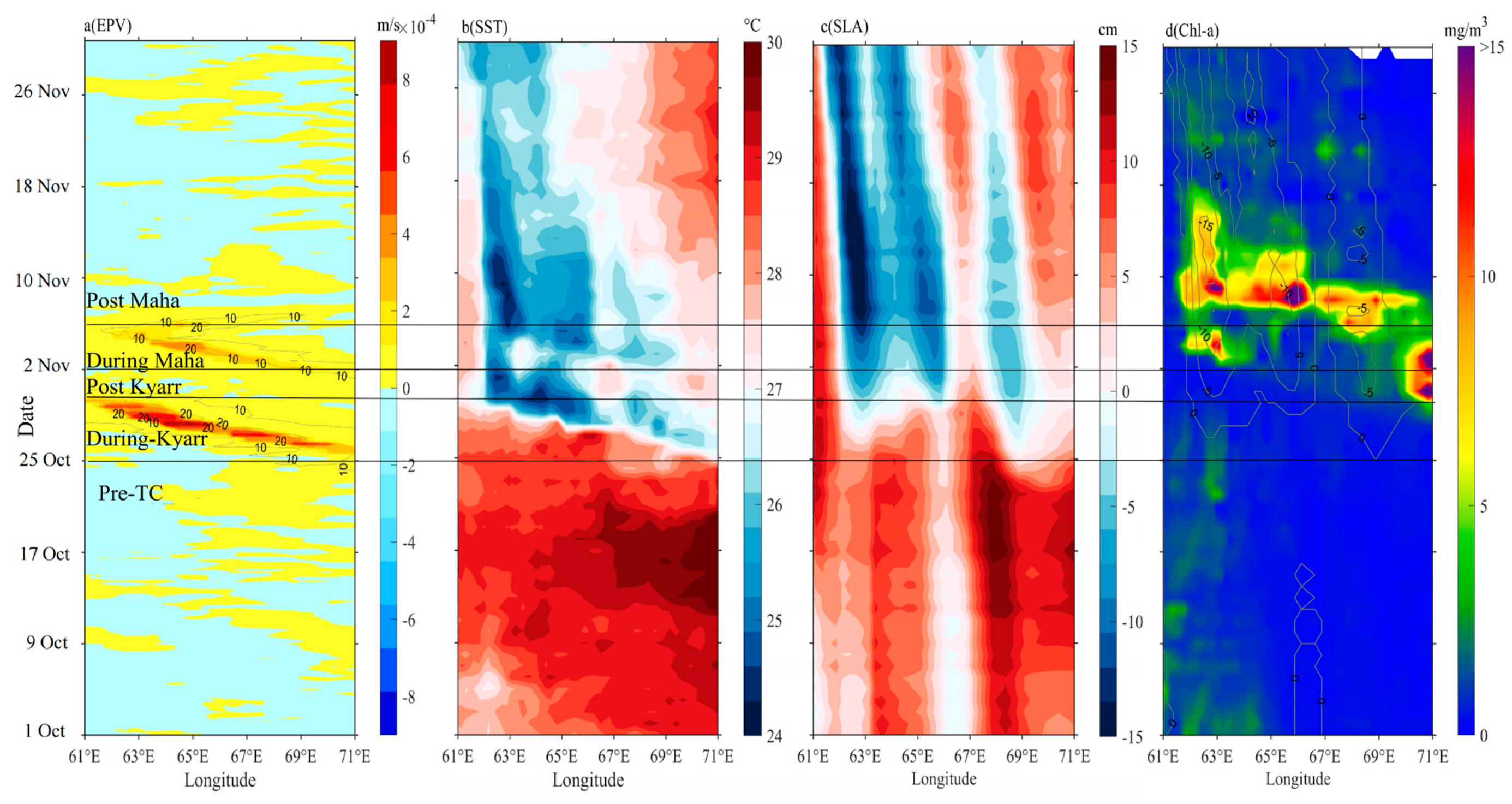
Based on the daily EPV, SST, SLA, and sea surface chl-a series (Figure 4), it was found that after the passage of the Kyarr and Maha, there were two cooling processes in the sea surface that temporally corresponded to two EPV peaks, with a lag of 1–2 days (Figure 4a,b). The cold eddies in the study area were generated (enhanced) by the strong EPVs during TC Kyarr (Maha) (Table 2). The maximum cooling (6 °C) and minimum SLA (−20 cm) appeared in cold eddy e3 from 6 November to 12 November (Figure 4b,c). The low SSTs and the high negative SLAs were maintained for more than 30 days due to eddy and Ekman pumping and water entrainment mixing induced by the TCs. As shown in Figure 4a,d, the increase in surface chl-a concentrations occurred 3 days later than the large EPVs. The surface chl-a concentrations had two short increasing periods. Six Bio-Argo floats (2902175, 2902205, 2902210, 2902202, 2902272, and 2902120) located in high-chl-a patches were selected to display the daily surface chl-a concentration variations. As shown in Figure 5, two short periods of increased surface chl-a concentrations were recorded at floats 2902175, 2902205, 2902210, 2902202, 2902272, and 2902120. The first period of higher surface chl-a concentrations occurred from late October to early November. A subsequent increase occurred from 4 to 10 November. The surface chl-a reduction identified between the post-Kyarr and post-Maha periods may have been related to the growth stage and vertical distribution of phytoplankton (Table 1). The physical mechanisms of these two chl-a increase events are explored in the next section.
3.3. Vertical Distributions of Temperature, Chl-a, and DO
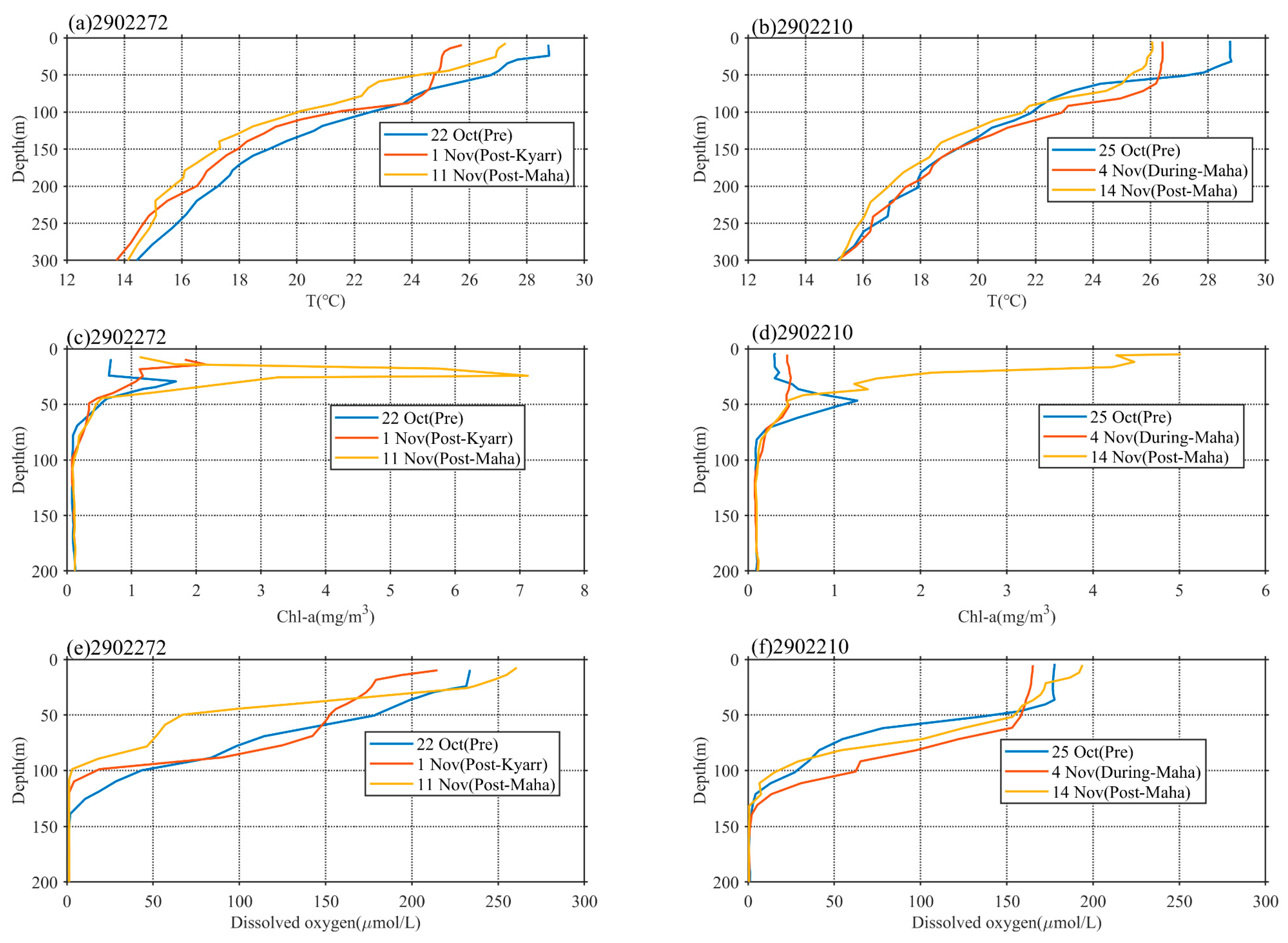
The data from two floats, 2902272 and 2902210 in e1 and e2, respectively, were used to further investigate phytoplankton variations in response to sequential TC forcing, as shown in Figure 6. The vertical profiles were recorded by two Bio-Argo floats, 2902272 and 2902210, located in the center of e1 and the edge of e2, respectively. Before the passage of TC Kyarr, the MLDs were 24.12 and 31.78 m at floats 2902272 and 2902210, respectively.
As recorded by float 2902272, on 1 November (approximately 4 days after the passage of TC Kyarr), the temperature in the upper mixed layer dropped by more than 2 °C, and the MLD deepened to 44.51 m, with the subsurface water temperatures increasing in the depth range of 78 to 95 m (Figure 6a). The water temperatures cooled in the depth ranges of 102 to 300 m and 5 to 78 m. The maximum chl-a concentration increased from 1.65 to 2.18 mg/m3, and the chl-a depth decreased from 28.57 to 14.28 m; this measurement may indicate that strong upwelling and vertical mixing changed the vertical distributions of temperature and chl-a. The DO decreased above a depth of 60 m and increased in the depth range of 60–82.9 m (Figure 6e). This can be explained by the water entrainment mechanism at the bottom of the mixed layer transporting the deeper low-DO waters to the layer above 60 m and the higher-DO waters downward to the layer below 60 m. On 11 November (approximately 6 days after the passage of TC Maha), the subsurface maximum chl-a concentration increased from 2.12 to 7.15 mg/m3 (Figure 6c), and the DO increased continuously above 22.85 m and decreased below 22.85 m. The former process was related to chl-a photosynthesis, whereas the latter may have been associated with the organic matter degradation process.
The area occupied by float 2902210 was affected by TC Kyarr (which had passed 5 days earlier) and TC Maha (which was currently passing through the area) on 4 November. TC Maha was closer to this float and located south of the float area. The mixed layer temperature also dropped by more than 2 °C, and the MLD extended to 58.53 m, with subsurface water temperatures increasing in the depth range of 52 to 132 m (Figure 6b). The temperature decrease measured in the mixed layer and increase measured in the subsurface layer were caused by entrainment mixing at the bottom of the mixed layer [27]. Simultaneously, a significant change in the vertical structure of chl-a was observed, and the subsurface maximum chl-a concentration decreased significantly while the chl-a concentrations in the depth ranges of 0 to 41 m and 80 to 120 m increased. This is the same driving mechanism associated with entrainment mixing at the bottom of the mixing layer discussed in the previous section; this mechanism caused the chl-a community to redistribute up and down in the subsurface layer. As discussed in the previous section, no active chl-a reproduction was observed before 4 November, and the vertical structure of chl-a was mainly controlled by vertical transport. The changes in DO recorded on 4 November are very interesting. The decrease (increase) in DO above a depth of 45 m (at depths of 45–130 m) was determined by physical redistribution processes. By 14 November, the situation had changed. The increased DO in the water layer above 45 m was related to the release of oxygen by chl-a photosynthesis, whereas the decreased DO levels in the water layer below 45 m may have been associated with reduced oxygen consumption by organisms. Phytoplankton growth was very active until 14 November; the subsurface maximum chl-a concentration increased from 0.45 to 5 mg/m3, and the peak chl-a depth moved upward toward the surface (Figure 6d). These changes indicate that entrainment by TCs can bring deep, nutrient-rich waters into the euphotic layer; under favorable light conditions, these nutrients can then be consumed by phytoplankton in the sunlit layer, leading to phytoplankton blooms, as observed after the passages of TCs Kyarr and Maha. In addition to bringing nutrients upward, entrainment can also transport phytoplankton from the euphotic layer to deeper layers, resulting in decreased phytoplankton in the euphotic layer and increased phytoplankton in both the surface and deep layers. The question arises: which is more important for the increase in sea-level chl-a concentrations: physical transport or biological biomass reproduction? This question will be clarified in the next section.
4. Discussion
The temporal and spatial scales of the cold eddies identified in this study are similar to those of the chl-a biomass patches (Figure 3), revealing the dynamic connection of phytoplankton growth with these eddies. The upwelling and entrainment induced by TCs may drive locally nutrient-rich waters upward into the euphotic layer. Investigations of the relative importance of different physical processes, such as upwelling, entrainment and nutrient supply-induced photosynthesis, in phytoplankton growth are vital for identifying the mechanisms driving phytoplankton blooms. Therefore, discussing the relative contributions of hydrodynamic processes and biological production is important. In this paper, we present observations of the evolution of the vertical water column structure during the passage of two subsequent TCs; the results show the clear responses of temperature, chl-a, and DO to these events. In this section, we discuss whether the observed increases in chl-a during the TCs were linked to in situ phytoplankton growth as a result of nutrient replenishment or simply to the redistribution of the subsurface phytoplankton community. Finally, we compare our results with those output by the biogeochemistry model.
4.1. Light and Nutrient Conditions in the Euphotic Layer before the TCs
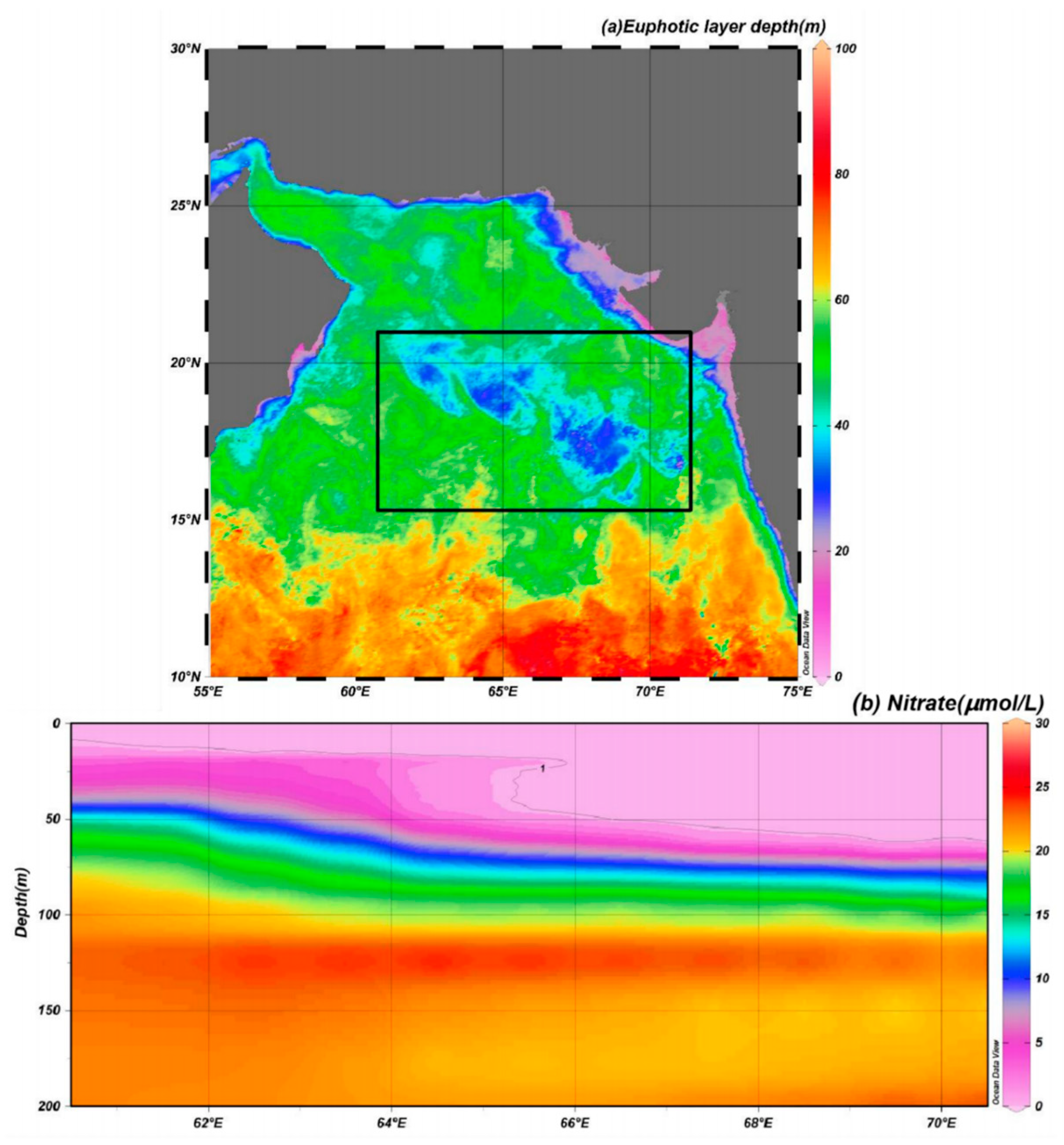
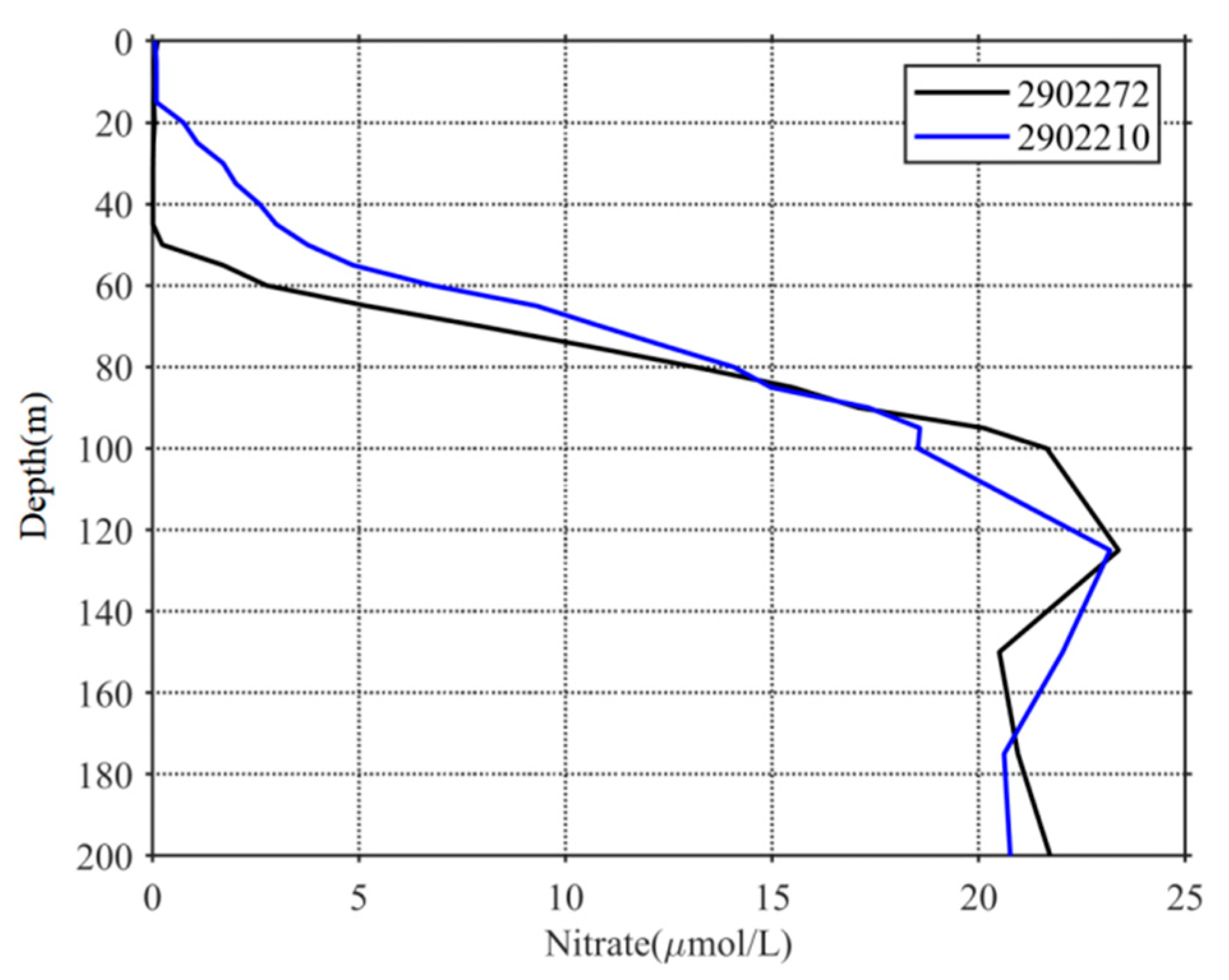
The upper sunlit layer of the ocean, known as the euphotic layer, is the most important factor regulating the growth of phytoplankton. Generally, active phytoplankton growth occurs due to the presence of sufficient nutrients and light in the euphotic layer. In this study, the light was not strong in high-chl-a areas compared with the surrounding waters after the studied TCs (Figure 7a), and the euphotic layer depths at the locations of floats 2902272 and 2902210 were 36.96 and 29.81 m, respectively; these values suggest that light was not the only factor limiting phytoplankton growth. In contrast, the monthly average euphotic-layer nitrate concentrations at floats 2902272 and 2902210 were 0.66 and 0.85 µmol/L, respectively, whereas much higher nitrate concentrations appeared below the euphotic layer (Figure 8). According to Nelson’s theory [44], 1 µmol/L is the nutrient threshold for phytoplankton growth. Thus, the nitrate level in the euphotic layer before the TCs may have been below this nitrate threshold and thus unfavorable for phytoplankton growth, leading to an oligotrophic environment (Figure 7b). TC forcing may have significantly changed this oligotrophic environment and played an important role in marine ecosystem dynamics.
4.2. The Translation Speed and Wind Speed of TCs Kyarr and Maha
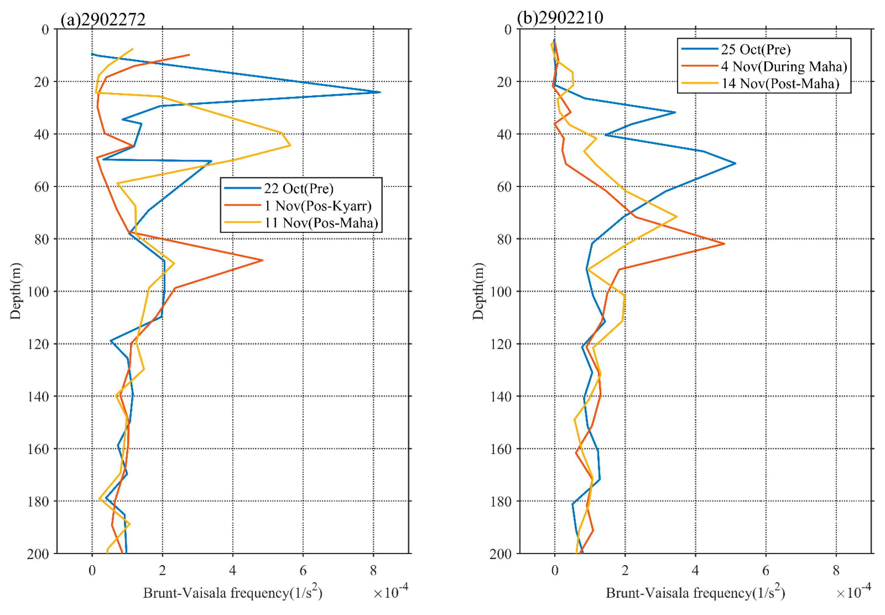
The translation speed and wind speed of a TC determine the forcing time to the upper ocean [41,45]. The forcing time can be considered the period during which wind speeds exceed 17 m/s along a TC path [4]. When the TC moves faster, the wind velocities on the right side of the TC path adopt a clockwise deflection that resonates with the near-inertial current to produce effective entrainment mixing [27,46,47]. Thus, a cold center is often observed at the surface, and subsequently, a cold tongue extending from this cold center can also be observed (Figure 4b). When the TC moves slowly, the forcing time of the TC on the upper ocean is longer, and the generated cooling area is generally located close to the TC path [1,2,26,48,49,50]. The vertical profiles of temperature and DO at the eddy center (float 2902272) after the passage of TC Kyarr clearly exhibited strong upwelling (with an uplifted isotherm) in the upper ocean (Figure 6a). Hence, slow-moving TCs tend to produce more persistent upwelling [1,51]. Notably, the slower a TC, the closer the cooling center to the TC path [50]. In our study, the strong TCs Kyarr and Maha moved at speeds of 3.4 and 3.8 m/s, respectively (Figure 2). The translation speed (Ts) of these TCs was thus closer to the phase speed (c1) of the first baroclinic mode (Froude number, Fr = Ts/c1~1, c1 = 2.9 m/s) [52,53]; therefore, right-side sea surface cooling and chl-a augments were attributed to both Ekman pumping and entrainment mixing at the base of the mixed layer. In addition, Huang and Oey [54] used a coupled biological-physical model to demonstrate that sub-mesoscale recirculation cells are very important for TC-induced right-side cooling and phytoplankton blooms, and that vertical mixing alone results in only weak asymmetry. The vertical buoyancy frequency (N2) profiles derived from the floats are shown in Figure 9. These physical processes induced the weakening of upper-ocean stratification (the maximum N2 values decreased from 8.2 × 10⁻⁴ to 4.8 × 10⁻⁴ and from 5.1 × 10⁻⁴ to 3.5 × 10⁻⁴), leading to the accumulation of phytoplankton after the passage of the TCs [55]. Both TCs moved at almost the same average speed, and TC Maha shifted backward to a deflection of nearly 150° on 5 November, thus extending the forcing time in the e3 area and possibly having a great impact on the upper ocean (Figure 10a). When the wind-stress forcing time is longer, more nutrient-rich cold water from the deeper layer can move upward to the surface layer. Therefore, when studying physical and biogeochemical responses to TCs, the intensity, translation speed, physical mechanism. and chl-a biomass reproduction associated with TCs must be comprehensively considered. The strong vertical mixing and upwelling caused by slow and strong sequential TCs can not only disrupt the vertical distribution of phytoplankton (e.g., inducing the first surface chl-a bloom after TC Kyarr), but can also transport nutrients into the euphotic layer (e.g., leading to the second surface chl-a bloom after TC Maha), and both led to two short chl-a blooms.
4.3. Impact of Physical Processes on Phytoplankton Enhancement in the Upper Ocean
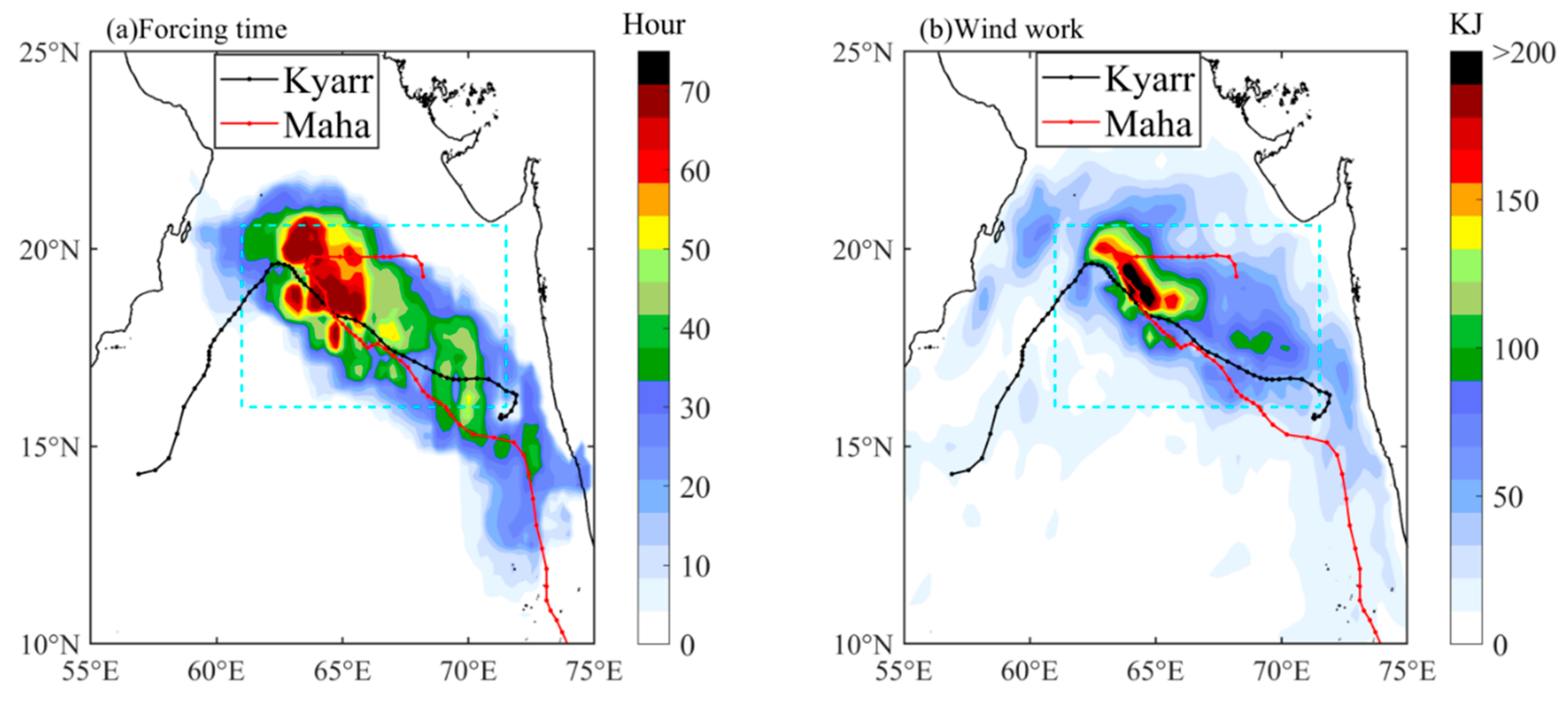
The forcing time increased gradually in the study area along the TC paths from south to north. The longest forcing time was approximately 65 h in e3; this period was longer than the inertial period (1/f = 36.75 h, where f is the local inertia frequency) (Figure 10a). The work done by wind stress (W) had a similar pattern to that of the forcing time, and the highest value was more than 200 kJ in e3 (Figure 10b). The wind-induced perturbation energy propagated downward through the near-inertial internal waves, resulting in strong water entrainment at the base of the mixed layer [46,56,57]. The long forcing time of the strong wind stress curl during the passages of Kyarr intensively contributed to the formation of the three cold eddies. The TC-induced cold eddies could have caused the horizontal exchange and vertical transportation of biochemical elements by physical processes (e.g., eddy pumping, eddy stirring, eddy trapping, and eddy–wind Ekman pumping) [58,59,60]. Liu et al. [61] found that eddy pumping caused by TC-induced cyclonic eddies was the most important physical process responsible for increasing surface chl-a concentrations rather than Ekman pumping or turbulent mixing following the passage of a TC. For sequential TCs with slow translation speeds and strong winds (estimated Fr values ranging from 1.2 to 1.4), the turbulence resulting from water entrainment mechanisms, together with eddy and Ekman pumping, caused upward nutrient fluxes that sustained chl-a biomass reproduction and water cooling in the mixed layer [23,62,63,64]. In addition to providing nutrient supplies, strong mixing also induced phytoplankton fluxes from the euphotic layer to the deep layer, leading to a decrease in phytoplankton in the euphotic layer. Simultaneously, the mixed-layer warm water was also transported by entrainment mixing to the deep layer, resulting in a temperature drop in the mixed layer and a temperature increase in the subsurface layer (Figure 6). The redistribution of phytoplankton in the upper ocean cannot change the total chl-a concentration. If chl-a production does not occur, the chl-a augmentation resulting from vertical redistribution may reduce the subsurface maximum chl-a concentration.
Whether a surface chl-a bloom is generated by the redistribution of phytoplankton with vertical gradients or by biological production is a key issue that must be considered when identifying the evolution and dynamics of surface chl-a blooms. Therefore, the depth-integrated chl-a was calculated to further clarify this difference. As observed by floats 2902272 and 2902210 (Figure 6), the chl-a profiles were approximately homogeneous below a depth of 100 m; thus, the depth-integrated chl-a concentrations were calculated over the upper 100 m depths. The depth-integrated chl-a concentrations obtained in the pre-TC, during-TC, and post-TC periods are listed in Table 1. During the first short period of surface chl-a enhancement, the depth-integrated chl-a concentrations changed from 51.3 to 60 mg/m2 and from 47.89 to 39.64 mg/m2 at floats 2902272 and 2902210, respectively. These changes imply that the chl-a distribution was mainly controlled by physical transport [24]. In contrast, the depth-integrated chl-a concentrations observed in the second bloom event reached 207.98 mg/m2 at float 2902272 and 117 mg/m2 at float 2902210, and substantial production occurred in the second event. Overall, these results confirm that in the post-TC Kyarr period, the major mechanism responsible for the surface chl-a bloom was subsurface phytoplankton redistribution, whereas for post-TC Maha, the major mechanism was phytoplankton production with turbulent mixing and upwelling-induced nutrient supplies in the surface layer.
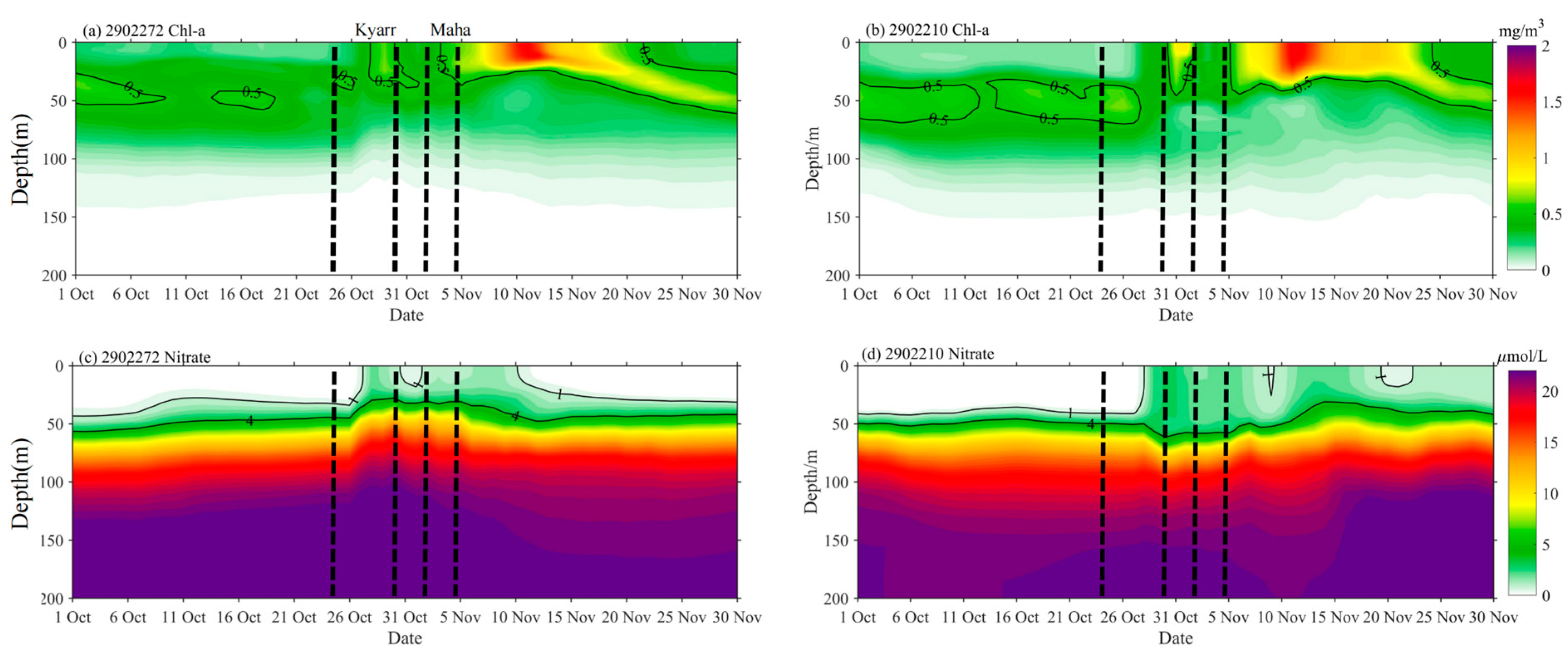
The biogeochemistry model products obtained for October and November are shown in Figure 11; the output temporal evolution of chl-a was consistent with the observations derived from the Bio-Argo floats. As shown in Figure 11, two short-period chl-a blooms can be found corresponding to TCs Kyarr and Maha. During the period of TC Kyarr, the depth-integrated chl-a (surface chl-a) concentrations changed from 35.67 mg/m2 (0.24 mg/m3) to 38.85 mg/m2 (0.63 mg/m3) at float 2902272 and from 39.14 mg/m2 (0.19 mg/m3) to 43.36 mg/m2 (0.86 mg/m3) at float 2902210 (Figure 12c,d). The first chl-a peak occurred on October 29th (31st) at float 2902272 (2902210). This phenomenon occurred because phytoplankton cells were redistributed by physical processes [24]. With vertical mixing and upwelling, the nitrate concentration in the surface water at float 2902272 (2902210) increased to 2.4 (3.8) µmol/L (Figure 11c,d). The nitrate concentration then began to decline as nutrient consumption and grazing increased in the restratified upper ocean, despite the nutrient-rich upper-ocean waters caused by the first TC. With the arrival of the second TC, the depth-integrated chl-a (surface chl-a) concentrations at floats 2902272 and 2902210 significantly increased to 50.09 mg/m2 (1.65 mg/m3) and 67.58 mg/m2 (1.72 mg/m3), respectively. These increases may have been attributed to biological biomass reproduction. Vertical mixing and upwelling (TC-induced Ekman pumping and eddy pumping) not only disrupted the balance between phytoplankton division and grazer consumption, thus reducing the encounter rates between phytoplankton and grazers, but also increased the nutrient supplies [65]. This resulted in more pronounced phytoplankton blooms lasting 20 days after the TC events.
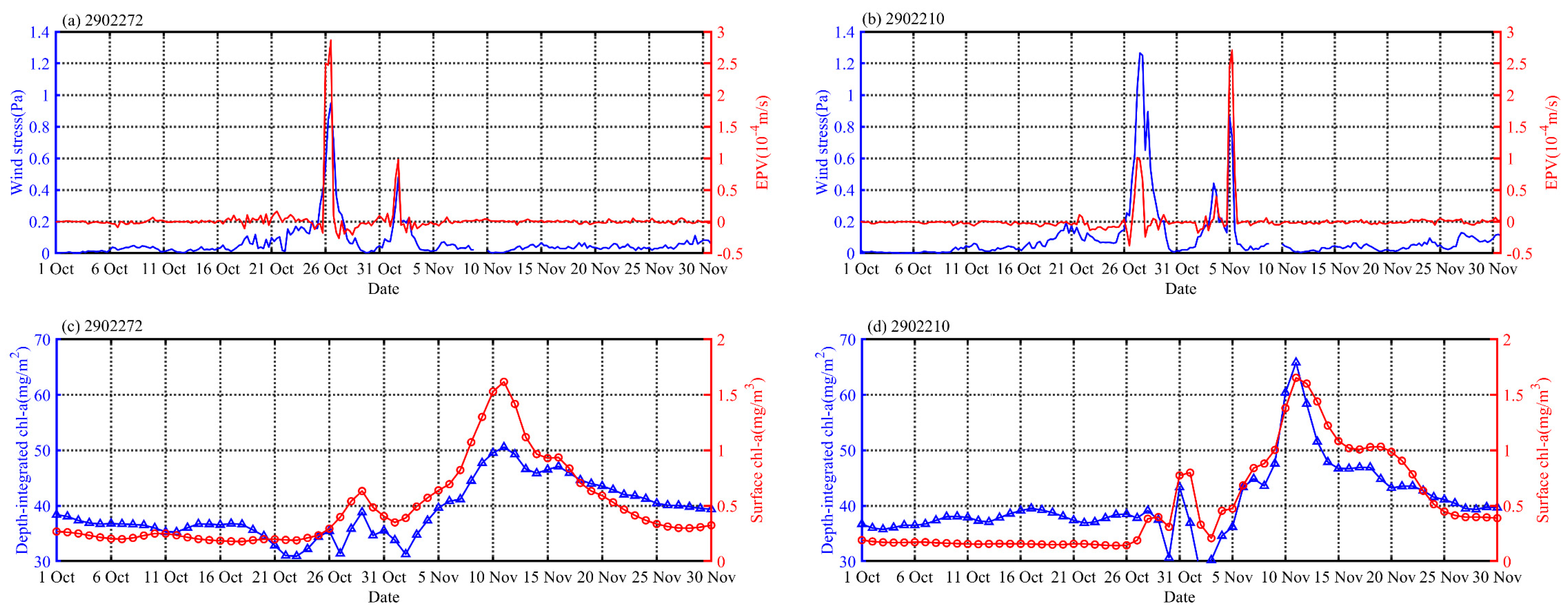
Combined with the model and float data, we can further quantify the contributions of different physical processes (upwelling and vertical mixing) to the vertical fluxes of nutrients at different locations along the TC paths. Interestingly, for float 2902272 (in the center of e1 and near the TC path), the model outputs showed that 1 (4) μmol/L nitrate isoline was uplifted to the surface (25 m) during TC Kyarr (strong EPV (2.8 × 10⁻⁴) and wind stress (0.9 Pa)) (Figure 11c and Figure 12a). This means that the upper ocean was dominated by strong upwelling rather than mixing. However, for float 2902210 (at the edge of e2 and on the right side of the TC path), the model outputs showed that 1 (4) μmol/L nitrate isoline was uplifted (deepened) to the surface (65 m) during TC Kyarr (weak EPV (9.1 × 10⁻⁵) and strong wind stress (1.3 Pa)) (Figure 11d and Figure 12b), indicating that strong vertical mixing rather than upwelling was the dominant process affecting nutrient resupply. This was because the current dynamics are different between the center of an eddy and the frontal edge of the eddy. The cyclonic wind stress of a TC increases the vorticity of the cyclonic eddy, so this relation is supported in the TC center; thus, pumping is the main driver, whereas vertical shear is a larger driver at the edge [66]. During the passage of TC Maha, the wind stress and EPV were 0.45 (0.92) Pa and 1 × 10⁻⁴ (2.7 × 10⁻⁴) m/s at the location of float 2902272 (2902210). The nitrate isoline of 4 μmol/L had no significant vertical displacement for float 2902272. However, for float 2902210, this isoline shifted from 56 to 47 m. These results imply that compared with TC Kyarr, at the 2902272 (2902210) location, the upper ocean in the center (edge) of e1 (e2) was dominated by weaker upwelling and mixing (stronger upwelling). These physical processes continued to maintain and enhance the upward transport of nutrients during the TC period.
5. Conclusions
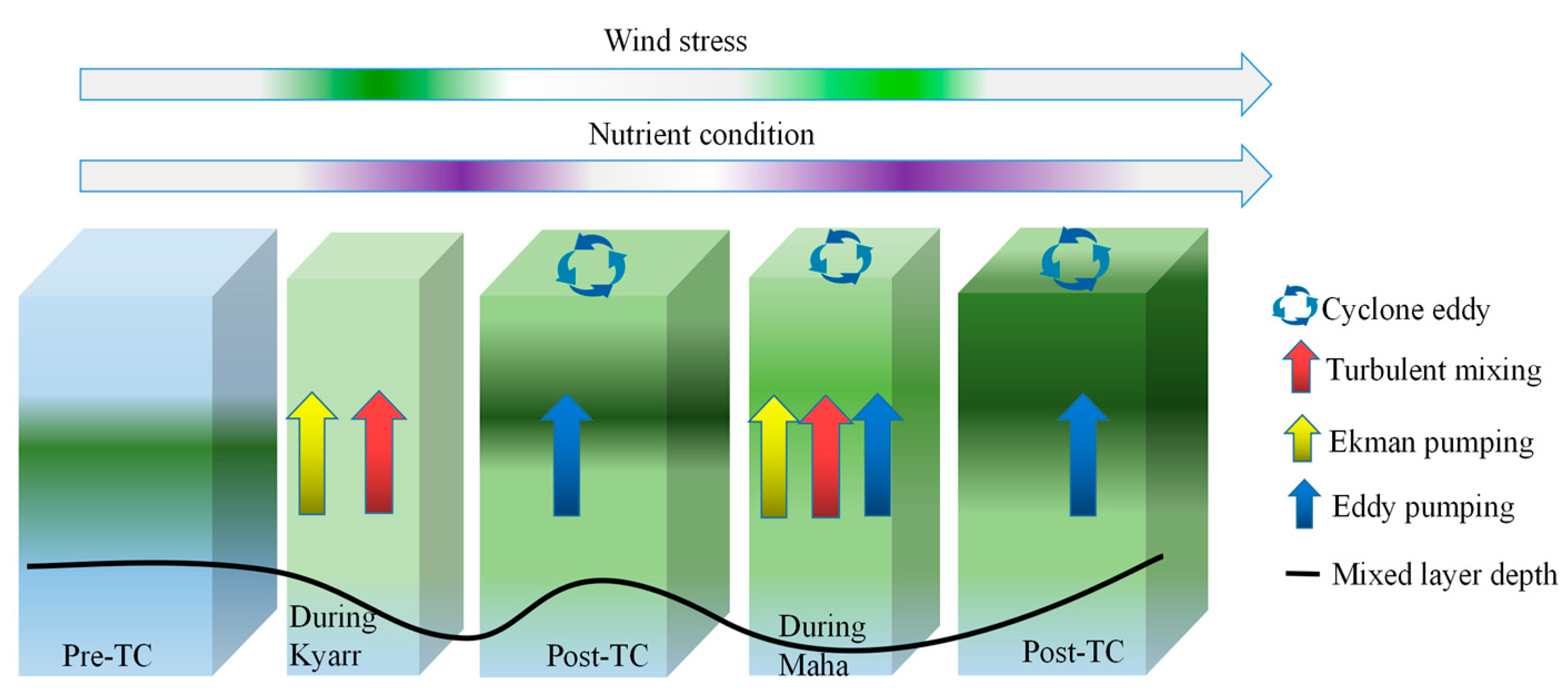
In this study, the upper-ocean physical and biochemical responses identified during sequential TCs Kyarr and Maha in the AS were investigated using satellite and Bio-Argo float datasets. Corresponding to the passages of the TCs, two cooling processes and two short chl-a blooms were identified on the sea surface with time intervals of 6–7 days. Three cold core eddies with SST decreases of more than 6 °C were induced by the TCs, as depicted from the Hovmollers. As summarized in Figure 13, the initial rapid increase in the surface chl-a concentration and decrease in the subsurface chl-a concentration were mainly caused by physical transport redistribution post-TC Kyarr, whereas the subsequent and more pronounced chl-a bloom in the upper ocean was due to net phytoplankton growth with nutrient-rich cold waters entering the euphotic layer by upwelling, entrainment mixing, and eddy pumping post-TC Maha. Upwelling (vertical mixing) was the dominant process by which nutrients near (on the right side of) the TC path were resupplied. The analyses of both the depth-integrated chl-a and biogeochemistry model data confirm these different mechanisms for phytoplankton blooms induced by sequential TCs.
Whether climate change will lead to an increase in the number of TCs remains uncertain, but warmer ocean temperatures and higher sea levels are expected to intensify. The strong winds associated with TCs initiate intense upwelling and mixing, resulting in enhanced phytoplankton biomass in the open ocean after the passage of a TC. Presently, quantitatively estimating phytoplankton dynamic responses to TCs in the upper ocean is difficult because low-frequency sample data fail to capture daily or weekly variabilities. Further high-frequency, in situ observations and more comprehensive conceptual and quantitative model simulations are required to explain the physical driving forces associated with TCs that modulate phytoplankton dynamics. Investigations of the role of such events on the short-term changes in this region’s phytoplankton dynamics should be the subject of future studies.
Author Contributions
Conceptualization, T.W. and S.Z.; methodology, T.W.; software, T.W.; validation, T.W., F.C., W.Z. and H.N.; formal analysis, T.W. and S.Z.; investigation, T.W., F.C., W.Z. and H.N.; resources, T.W.; data curation, T.W. and S.Z.; writing—Original draft preparation, T.W.; writing—Review and editing, S.Z., F.C., J.P. and A.T.D.; visualization, T.W., H.N. and W.Z.; supervision, S.Z. and J.P.; project administration, S.Z. and J.P.; funding acquisition, S.Z. and J.P. All authors have read and agreed to the published version of the manuscript.
Funding
This research was funded by Scientific Research Start-Up Foundation of Shantou University (NTF20006), Innovation and Entrepreneurship Project of Shantou (2021112176541391), Guangdong Natural Science Foundation of China (2016A030312004), National Natural Science Foundation of China (U1901213, 40876005, 41676008) and Scientific Research Start-Up Foundation of Jiangxi Normal University and the General Research Fund of Hong Kong Research Grants Council (RGC) (CUHK 14303818). We sincerely thank the anonymous reviewers for their valuable constructive comments that helped to improve our manuscript.
Institutional Review Board Statement
Not applicable.
Informed Consent Statement
Not applicable.
Data Availability Statement
The in situ chl-a, dissolved oxygen, temperature, and salinity data were obtained from the India Argo project (ftp://ftp.ifremer.fr/ifremer/argo (accessed on 5 April 2021)). The wind data and SST data are available at Remote Sensing Systems (ftp://ftp.remss.com/ccmp/v02.0/ (accessed on 1 April 2021) and ftp://ftp.remss.com/sst/daily/ (accessed on 1 April 2021)). The PAR data were obtained from GlobColor’s Working Group (http://hermes.acri.fr (accessed on 1 April 2021)). The climatological nitrate data are available at the National Oceanic and Atmospheric Administration (NOAA). The surface chl-a, SLA, geostrophic velocity, and model data are available at the CMEMS website (http://marine.copernicus.eu/ (accessed on 1 April 2021)). We sincerely thank the anonymous reviewers for their valuable constructive comments that helped to improve our manuscript.
Conflicts of Interest
The authors declare no conflict of interest.
References
- Price, J.F. Upper Ocean response to a hurricane. J. Phys. Oceanogr. 1981, 11, 153–175. [Google Scholar] [CrossRef] [Green Version]
- Chu, P.C.; Veneziano, J.M.; Fan, C.; Carron, M.J.; Liu, W.T. Response of the South China Sea to tropical cyclone Ernie 1996. J. Geophys. Res. Ocean. 2000, 105, 13991–14009. [Google Scholar] [CrossRef] [Green Version]
- Davis, A.; Yan, X.H. Hurricane forcing on chlorophyll-a concentration off the northeast coast of the US. Geophys. Res. Lett. 2004, 31, L17304. [Google Scholar] [CrossRef]
- Sun, L.; Li, Y.X.; Yang, Y.J.; Wu, Q.; Chen, X.T.; Li, Q.Y.; Xian, T. Effects of super typhoons on cyclonic ocean eddies in the western North Pacific: A satellite data-based evaluation between 2000 and 2008. J. Geophys. Res. Ocean. 2014, 119, 5585–5598. [Google Scholar] [CrossRef]
- Price, J.F.; Sanford, T.B.; Forristall, G.Z. Forced stage response to a moving hurricane. J. Phys. Oceanogr. 1994, 24, 233–260. [Google Scholar] [CrossRef]
- Wentz, F.J.; Gentemann, C.; Smith, D.; Chelton, D. Satellite measurements of sea surface temperature through clouds. Science 2000, 288, 847–850. [Google Scholar] [CrossRef] [PubMed] [Green Version]
- Black, W.J.; Dickey, T.D. Observations and analyses of upper ocean responses to tropical storms and hurricanes in the vicinity of Bermuda. J. Geophys. Res. Ocean. 2008, 113, C08009. [Google Scholar] [CrossRef] [Green Version]
- D’Asaro, E.A.; Black, P.G.; Centurioni, L.R.; Chang, Y.T.; Chen, S.S.; Foster, R.C.; Lin, I.I. Impact of typhoons on the ocean in the Pacific. Bull. Am. Meteorol. Soc. 2014, 95, 1405–1418. [Google Scholar] [CrossRef]
- Chiang, T.L.; Wu, C.R.; Oey, L.Y. Typhoon Kai-Tak: An ocean’s perfect storm. J. Phys. Oceanogr. 2011, 41, 221–233. [Google Scholar] [CrossRef]
- Soloviev, A.V.; Lukas, R.; Donelan, M.A.; Haus, B.K.; Ginis, I. The air-sea interface and surface stress under tropical cyclones. Sci. Rep. 2014, 4, 5306. [Google Scholar] [CrossRef] [PubMed]
- Soloviev, A.V.; Lukas, R.; Donelan, M.A.; Haus, B.K.; Ginis, I. Is the state of the air-sea interface a factor in rapid intensification and rapid decline of tropical cyclones? J. Geophys. Res. Ocean. 2017, 122, 10174–10183. [Google Scholar] [CrossRef]
- Park, J.H.; Yeo, D.E.; Lee, K.; Lee, H.; Lee, S.W.; Noh, S.; Nam, S. Rapid decay of slowly moving Typhoon Soulik (2018) due to interactions with the strongly stratified northern East China Sea. Geophys. Res. Lett. 2019, 46, 14595–14603. [Google Scholar] [CrossRef] [Green Version]
- Shay, L.K.; Uhlhorn, E.W. Loop current response to Hurricanes Isidore and Lili. Mon. Weather. Rev. 2008, 136, 3248–3274. [Google Scholar] [CrossRef] [Green Version]
- Li, J.; Zheng, H.; Xie, L.; Zheng, Q.; Ling, Z.; Li, M. Response of Total Suspended Sediment and Chlorophyll-a Concentration to Late Autumn Typhoon Events in the Northwestern South China Sea. Remote Sens. 2021, 13, 2863. [Google Scholar] [CrossRef]
- Naik, H.; Naqvi, S.W.A.; Suresh, T.; Narvekar, P.V. Impact of a tropical cyclone on biogeochemistry of the central Arabian Sea. Glob. Biogeochem. Cycles 2008, 22, GB3020. [Google Scholar] [CrossRef]
- Byju, P.; Kumar, S.P. Physical and biological response of the Arabian Sea to tropical cyclone Phyan and its implications. Mar. Environ. Res. 2011, 71, 325–330. [Google Scholar] [CrossRef] [PubMed] [Green Version]
- Gaube, P.; Chelton, D.B.; Strutton, P.G.; Behrenfeld, M.J. Satellite observations of chlorophyll, phytoplankton biomass, and Ekman pumping in nonlinear mesoscale eddies. J. Geophys. Res. Ocean. 2013, 118, 6349–6370. [Google Scholar] [CrossRef] [Green Version]
- Girishkumar, M.S.; Thangaprakash, V.P.; Udaya Bhaskar, T.V.S.; Suprit, K.; Sureshkumar, N.; Baliarsingh, S.K.; Shivaprasad, S. Quantifying tropical cyclone’s effect on the biogeochemical processes using profiling float observations in the Bay of Bengal. J. Geophys. Res. Ocean. 2019, 124, 1945–1963. [Google Scholar] [CrossRef]
- Subrahmanyam, B.; Rao, K.H.; Srinivasa Rao, N.; Murty, V.S.N.; Sharp, R.J. Influence of a tropical cyclone on chlorophyll-a concentration in the Arabian Sea. Geophys. Res. Lett. 2002, 29, 2065. [Google Scholar] [CrossRef]
- Pan, J.; Huang, L.; Devlin, A.T.; Lin, H. Quantification of typhoon-induced phytoplankton blooms using satellite multi-sensor data. Remote Sens. 2018, 10, 318. [Google Scholar] [CrossRef] [Green Version]
- Ye, H.J.; Sui, Y.; Tang, D.L.; Afanasyev, Y.D. A subsurface chlorophyll a bloom induced by typhoon in the South China Sea. J. Mar. Syst. 2013, 128, 138–145. [Google Scholar] [CrossRef]
- Pan, S.; Shi, J.; Gao, H.; Guo, X.; Yao, X.; Gong, X. Contributions of physical and biogeochemical processes to phytoplankton biomass enhancement in the surface and subsurface layers during the passage of typhoon Damrey. J. Geophys. Res. Biogeosci. 2017, 122, 212–229. [Google Scholar] [CrossRef]
- Wang, T.; Zhang, S.; Chen, F.; Ma, Y.; Jiang, C.; Yu, J. Influence of sequential tropical cyclones on phytoplankton blooms in the northwestern South China Sea. J. Oceanol. Limnol. 2021, 39, 14–25. [Google Scholar] [CrossRef]
- Chai, F.; Wang, Y.; Xing, X.; Yan, Y.; Xue, H.; Wells, M.; Boss, E. A limited effect of sub-tropical typhoons on phytoplankton dynamics. Biogeosciences 2021, 18, 849–859. [Google Scholar] [CrossRef]
- Lin, I.; Liu, W.T.; Wu, C.C.; Wong, G.T.; Hu, C.; Chen, Z.; Liu, K.K. New evidence for enhanced ocean primary production triggered by tropical cyclone. Geophys. Res. Lett. 2003, 30, 1718. [Google Scholar] [CrossRef] [Green Version]
- Sun, L.; Yang, Y.J.; Xian, T.; Lu, Z.M.; Fu, Y.F. Strong enhancement of chlorophyll a concentration by a weak typhoon. Mar. Ecol. Prog. Ser. 2010, 404, 39–50. [Google Scholar] [CrossRef]
- Zhang, S.; Xie, L.; Hou, Y.; Zhao, H.; Qi, Y.; Yi, X. Tropical storm-induced turbulent mixing and chlorophyll-a enhancement in the continental shelf southeast of Hainan Island. J. Mar. Syst. 2014, 129, 405–414. [Google Scholar] [CrossRef] [Green Version]
- Lee, C.M.; Jones, B.H.; Brink, K.H.; Fischer, A.S. The upper-ocean response to monsoonal forcing in the Arabian Sea: Seasonal and spatial variability. Deep. Sea Res. Part II Trop. Stud. Oceanogr. 2000, 47, 1177–1226. [Google Scholar] [CrossRef]
- Fischer, A.S.; Weller, R.A.; Rudnick, D.L.; Eriksen, C.C.; Lee, C.M.; Brink, K.H.; Leben, R.R. Mesoscale eddies, coastal upwelling, and the upper-ocean heat budget in the Arabian Sea. Deep. Sea Res. Part II Trop. Stud. Oceanogr. 2002, 49, 2231–2264. [Google Scholar] [CrossRef]
- Evan, A.T.; Camargo, S.J. A climatology of Arabian Sea cyclonic storms. J. Clim. 2011, 24, 140–158. [Google Scholar] [CrossRef] [Green Version]
- Dube, S.K.; Rao, A.D.; Sinha, P.C.; Murty, T.S.; Bahulayan, N. Storm surge in the Bay of Bengal and Arabian Sea the problem and its prediction. Mausam 1997, 48, 283–304. [Google Scholar] [CrossRef]
- Kuttippurath, J.; Sunanda, N.; Martin, M.V.; Chakraborty, K. Tropical storms trigger phytoplankton blooms in the deserts of north Indian Ocean. Clim. Atmos. Sci. 2021, 4, 1–12. [Google Scholar] [CrossRef]
- Murakami, H.; Vecchi, G.A.; Underwood, S. Increasing frequency of extremely severe cyclonic storms over the Arabian Sea. Nat. Clim. Chang. 2017, 7, 885–889. [Google Scholar] [CrossRef]
- Da, N.D.; Foltz, G.R.; Balaguru, K. Observed Global Increases in Tropical Cyclone-Induced Ocean Cooling and Primary Production. Geophys. Res. Lett. 2021, 48, e2021GL092574. [Google Scholar] [CrossRef]
- Maritorena, S.; d’Andon, O.H.F.; Mangin, A.; Siegel, D.A. Merged satellite ocean colordata products using a bio-optical model: Characteristics, benefits and issues. Remote Sens. Environ. 2010, 114, 1791–1804. [Google Scholar] [CrossRef]
- Garver, S.A.; Siegel, D.A. Inherent optical property inversion of ocean color spectra and its biogeochemical interpretation: 1. Time series from the Sargasso Sea. J. Geophys. Res. Ocean. 1997, 102, 18607–18625. [Google Scholar] [CrossRef]
- Aumont, O.; Éthé, C.; Tagliabue, A.; Bopp, L.; Gehlen, M. PISCES-v2: An ocean biogeochemical model for carbon and ecosystem studies. Geosci. Model Dev. 2015, 8, 2465–2513. [Google Scholar] [CrossRef] [Green Version]
- Lellouche, J.M.; Greiner, E.; Galloudec, O.L.; Garric, G.; Regnier, C.; Drevillon, M.; Traon, P.Y.L. Recent updates to the Copernicus Marine Service global ocean monitoring and forecasting real-time 1/12° high-resolution system. Ocean. Sci. 2018, 14, 1093–1126. [Google Scholar] [CrossRef] [Green Version]
- Powell, M.D.; Vickery, P.J.; Reinhold, T.A. Reduced drag coefficient for high wind speeds in tropical cyclones. Nature 2003, 422, 279–283. [Google Scholar] [CrossRef] [PubMed]
- de Boyer Montégut, C.; Madec, G.; Fischer, A.S.; Lazar, A.; Iudicone, D. Mixed layer depth over the global ocean: An examination of profile data and a profile-based climatology. J. Geophys. Res. Ocean. 2004, 109, C12003. [Google Scholar] [CrossRef]
- Rochford, P.A.; Kara, A.B.; Wallcraft, A.J.; Arnone, R.A. Importance of solar subsurface heating in ocean general circulation models. J. Geophys. Res. Ocean. 2001, 106, 30923–30938. [Google Scholar] [CrossRef]
- Mei, W.; Pasquero, C.; Primeau, F. The effect of translation speed upon the intensity of tropical cyclones over the tropical ocean. Geophys. Res. Lett. 2012, 39, L07801. [Google Scholar] [CrossRef] [Green Version]
- Wu, R.; Li, C. Upper ocean response to the passage of two sequential typhoons. Deep. Sea Res. Part I Oceanogr. Res. Pap. 2018, 132, 68–79. [Google Scholar] [CrossRef]
- Nelson, D.M.; Smith, W., Jr. Sverdrup revisited: Critical depths, maximum chlorophyll levels, and the control of Southern Ocean productivity by the irradiance-mixing regime. Limnol. Oceanogr. 1991, 36, 1650–1661. [Google Scholar] [CrossRef]
- Zhao, H.; Wang, Y. Phytoplankton increases induced by tropical cyclones in the South China Sea during 1998–2015. J. Geophys. Res. Ocean. 2018, 123, 2903–2920. [Google Scholar] [CrossRef]
- Zhang, H.; Chen, D.; Zhou, L.; Liu, X.; Ding, T.; Zhou, B. Upper Ocean response to typhoon Kalmaegi (2014). J. Geophys. Res. Ocean. 2016, 121, 6520–6535. [Google Scholar] [CrossRef]
- Busireddy, N.K.R.; Ankur, K.; Osuri, K.K.; Sivareddy, S.; Niyogi, D. The response of ocean parameters to tropical cyclones in the Bay of Bengal. Q. J. R. Meteorol. Soc. 2019, 145, 3320–3332. [Google Scholar] [CrossRef] [Green Version]
- Shay, L.K.; Goni, G.J.; Black, P.G. Effects of a warm oceanic feature on Hurricane Opal. Mon. Weather. Rev. 2000, 128, 1366–1383. [Google Scholar] [CrossRef]
- Liu, X.; Wang, M.; Shi, W. A study of a Hurricane Katrina–induced phytoplankton bloom using satellite observations and model simulations. J. Geophys. Res. Ocean. 2008, 114. [Google Scholar] [CrossRef] [Green Version]
- Mei, W.; Pasquero, C. Spatial and temporal characterization of sea surface temperature response to tropical cyclones. J. Clim. 2013, 26, 3745–3765. [Google Scholar] [CrossRef]
- Stramma, L.; Cornillon, P.; Price, J.F. Satellite observations of sea surface cooling by hurricanes. J. Geophys. Res. Ocean. 1986, 91, 5031–5035. [Google Scholar] [CrossRef]
- Geisler, J.E. Linear theory of the response of a two-layer ocean to a moving hurricane. Geophys. Astrophys. Fluid Dyn. 1970, 1, 249–272. [Google Scholar] [CrossRef]
- Chang, Y.C.; Tseng, R.S.; Chu, P.C.; Chen, J.M.; Centurioni, L.R. Observed strong currents under global tropical cyclones. J. Mar. Syst. 2016, 159, 33–40. [Google Scholar] [CrossRef] [Green Version]
- Huang, S.M.; Oey, L.Y. Right-side cooling and phytoplankton bloom in the wake of a tropical cyclone. J. Geophys. Res. Ocean. 2015, 120, 5735–5748. [Google Scholar] [CrossRef]
- Niu, L.; van Gelder, P.H.A.J.M.; Zhang, C.; Guan, Y.; Vrijling, J.K. Physical control of phytoplankton bloom development in the coastal waters of Jiangsu (China). Ecol. Model. 2016, 321, 75–83. [Google Scholar] [CrossRef]
- Large, W.G.; McWilliams, J.C.; Doney, S.C. Oceanic vertical mixing: A review and a model with a nonlocal boundary layer parameterization. Rev. Geophys. 1994, 32, 363–403. [Google Scholar] [CrossRef] [Green Version]
- Jaimes, B.; Shay, L.K. Mixed layer cooling in mesoscale oceanic eddies during Hurricanes Katrina and Rita. Mon. Weather. Rev. 2009, 137, 4188–4207. [Google Scholar] [CrossRef] [Green Version]
- Chelton, D.B.; Gaube, P.; Schlax, M.G.; Early, J.J.; Samelson, R.M. The influence of nonlinear mesoscale eddies on near-surfaceoceanic chlorophyll. Science 2011, 334, 328–332. [Google Scholar] [CrossRef]
- Chang, Y.L.; Miyazawa, Y.; Oey, L.Y.; Kodaira, T.; Huang, S. The formation processes of phytoplankton growth and decline in mesoscale eddies in the western North Pacific Ocean. J. Geophys. Res. Ocean. 2017, 122, 4444–4455. [Google Scholar] [CrossRef]
- Wang, T.; Du, Y.; Liao, X.; Xiang, C. Evidence of Eddy-Enhanced Winter Chlorophyll-a Blooms in Northern Arabian Sea: 2017 Cruise Expedition. J. Geophys. Res. Ocean. 2020, 125, e2019JC015582. [Google Scholar] [CrossRef]
- Liu, Y.; Tang, D.; Evgeny, M. Chlorophyll concentration response to the typhoon wind-pump induced upper ocean processes considering air–sea heat exchange. Remote Sens. 2019, 11, 1825. [Google Scholar] [CrossRef] [Green Version]
- Williams, C.; Sharples, J.; Mahaffey, C.; Rippeth, T. Wind-driven nutrient pulses to the subsurface chlorophyll maximum in seasonally stratified shelf seas. Geophys. Res. Lett. 2013, 40, 5467–5472. [Google Scholar] [CrossRef] [Green Version]
- Lee, K.; Matsuno, T.; Endoh, T.; Ishizaka, J.; Zhu, Y.; Takeda, S.; Sukigara, C. A role of vertical mixing on nutrient supply into the subsurface chlorophyll maximum in the shelf region of the East China Sea. Cont. Shelf Res. 2016, 143, 139–150. [Google Scholar] [CrossRef]
- Du, C.; Liu, Z.; Kao, S.J.; Dai, M. Diapycnal fluxes of nutrients in an oligotrophic oceanic regime: The South China Sea. Geophys. Res. Lett. 2017, 44, 11–510. [Google Scholar] [CrossRef]
- Behrenfeld, M.J.; Boss, E.S. Resurrecting the Ecological Underpinnings of Ocean Plankton Blooms. Annu. Rev. Mar. Sci. 2014, 6, 167–208. [Google Scholar] [CrossRef] [Green Version]
- Jaimes, B.; Shay, L.K.; Halliwell, G.R. The response of quasigeostrophic oceanic vortices to tropical cyclone forcing. J. Phys. Oceanogr. 2011, 41, 1965–1985. [Google Scholar] [CrossRef]
Figure 1.
The study area (black rectangle) in the Arabian Sea (AS). The paths of the two sequential TCs in 2019; the black and orange lines represent the tracks of TCs Kyarr and Maha, respectively. The interval between adjacent circles is 6 h, and the color of the circle indicates the intensity of the TC. The dotted lines represent the location of the cold eddies e1, e2, and e3 (1 November 2019–7 November 2019). The Bio-Argo floats are represented by various colored symbols, 6 Bio-Argo floats were selected among them. The small (large) symbols represent the location of Bio-Argo floats during pre (post)-TC Kyarr.

Figure 2.
Translation speed and maximum wind speed of TCs Kyarr and Maha.

Figure 3.
Spatial and temporal distributions of (a1–a5) wind speed (arrow) and EPV (shadow area), (b1–b5) SST, (c1–c5) SLA and geostrophic current (arrow), and (d1–d5) sea surface concentrations of chl-a derived from remote sensing data for 20 October–19 November 2019, overlaid with SLA contours (solid-positive and dashed-negative). e1, e2, and e3 in (c2–c5) denote the three cold eddies. The box represents the study area, and the thick black lines represent the paths of TCs Kyarr and Maha.

Figure 4.
Daily variations in (a) EPV, (b) SST, (c) SLA, and (d) sea surface chl-a concentration along the tracks of the TC Kyarr from 1 October to 30 November. The contour lines represent integer EPV and SLA in (a,d), respectively. Time is divided by four black lines into five periods (Pre-TC: before 25 October; During Kyarr: 26 October to 30 October; Post Kyarr: 1 November to 2 November; During Maha: 2 November to 5 November; Post Maha: after 5 November).

Figure 5.
Two short periods of surface chl-a enhancement were derived from remote sensing data at 2902175, 2902205, 2902210, 2902202, 2902272, and 2902120.
Figure 5.
Two short periods of surface chl-a enhancement were derived from remote sensing data at 2902175, 2902205, 2902210, 2902202, 2902272, and 2902120.

Figure 6.
In situ vertical profiles of temperature (a,b), chl-a concentration (c,d), and dissolved oxygen concentrations (e,f) at Bio-Argo floats 2902272 and 2902210.
Figure 6.
In situ vertical profiles of temperature (a,b), chl-a concentration (c,d), and dissolved oxygen concentrations (e,f) at Bio-Argo floats 2902272 and 2902210.

Figure 7.
(a) Spatial distribution of the average euphotic layer depth after sequential TCs Kyarr and Maha (6 November–10 November); (b) nitrate distribution profile by WOA 18 along the axial TC path transect in the AS during October 2019. The black rectangle represents the study area.
Figure 7.
(a) Spatial distribution of the average euphotic layer depth after sequential TCs Kyarr and Maha (6 November–10 November); (b) nitrate distribution profile by WOA 18 along the axial TC path transect in the AS during October 2019. The black rectangle represents the study area.

Figure 8.
Vertical distribution of nitrates in October based on WOA 18 datasets.

Figure 9.
Vertical profiles of buoyancy frequency from Bio-Argo floats.

Figure 10.
The spatial forcing time (a) and wind work (b) in the AS during the sequential TCs.

Figure 11.
Time series of chl-a (a,b) and nitrate (c,d) concentrations based on the biogeochemistry model product in October and November in the areas of floats 2902272 and 2902210. Time is divided by four black lines into five periods (Pre-TC: before 25 October; During Kyarr: 26 October to 30 October; Post Kyarr: 1 November to 2 November; During Maha: 2 November to 5 November; Post Maha: after 5 November).

Figure 12.
Time series of wind stress and EPV (a,b), and depth-integrated chl-a and surface chl-a (c,d) based on the biogeochemistry model product in October and November in the areas of floats 2902272 and 2902210.
Figure 12.
Time series of wind stress and EPV (a,b), and depth-integrated chl-a and surface chl-a (c,d) based on the biogeochemistry model product in October and November in the areas of floats 2902272 and 2902210.

Figure 13.
A schematic sketch of the upper ocean biological response (vertical chl-a) to sequential TC events.
Figure 13.
A schematic sketch of the upper ocean biological response (vertical chl-a) to sequential TC events.


Table 1.
Statistical results of the Bio-Argo floats.
| Location | e1 | e2 | ||||
|---|---|---|---|---|---|---|
| Argo | 2902272 | 2902210 | ||||
| Period | Pre-TC (22 October) | Post Kyarr (1 November) | Post Maha (11 November) | Pre-TC (25 October) | During Maha (4 November) | Post Maha (14 November) |
| Surface chl-a (mg/m3) | 0.67 | 1.7 | 1.12 | 0.3 | 0.45 | 4.97 |
| Max chl-a (mg/m3)/depth (m) | 1.68/29 | 2.1/20 | 7.12/24 | 1.26/47 | 0.50/26 | 5/9 |
| Integrate chl-a (mg/m2) | 51.3 | 60 | 131.01 | 47.89 | 39.64 | 117 |
| MLD (m)/variance (m) | 24.12/5.2 | 44.51/7.6 | 25.69/4.5 | 31.78/6.2 | 58.53/6.9 | 30.67/5.4 |
| EPV (m/s) (period) | 2.3 × 10⁻⁵ (Pre-TC) | 2.8 × 10⁻⁴ (During Kyarr) | 1.0 × 10⁻⁴ (During Maha) | 1.8 × 10⁻⁵ (Pre-TC) | 9.1 × 10⁻⁵ (During Kyarr) | 2.7 × 10⁻⁴ (During Maha) |
| Total wind work (KJ) | 72 | 85 | ||||
| Total forcing time (hour) | 36 | 57 | ||||
Note that Pre-TC: before 25 October; During Kyarr: 26 October to 30 October; Post Kyarr: 1 November to 2 November; During Maha: 2 November to 5 November; and Post Maha: after 6 November. The depth-integrated chl-a is calculated over the upper 100 m depth.
Table 2.
Statistical characteristics of the three cold eddies.
| Eddy | Radius (km) | Maximum Geostrophic Current (m/s) | Maximum SST Cooling (°C) | Minimum SLA (cm) | Maximum Chl-a (mg/m3) | Maximum EPV (m/s) |
|---|---|---|---|---|---|---|
| e1 | 166.5 | 0.59 | −3.95 | −7.26 | 12.76 | 8.1 × 10⁻⁴ |
| e2 | 175.2 | 0.56 | −5.28 | −14.27 | 23.09 | 9.3 × 10⁻⁴ |
| e3 | 186.4 | 0.75 | −5.47 | −20.56 | 16.51 | 6.9 × 10⁻⁴ |
Publisher’s Note: MDPI stays neutral with regard to jurisdictional claims in published maps and institutional affiliations. |
© 2022 by the authors. Licensee MDPI, Basel, Switzerland. This article is an open access article distributed under the terms and conditions of the Creative Commons Attribution (CC BY) license (https://creativecommons.org/licenses/by/4.0/).
Share and Cite
MDPI and ACS Style
Wang, T.; Chen, F.; Zhang, S.; Pan, J.; Devlin, A.T.; Ning, H.; Zeng, W. Physical and Biochemical Responses to Sequential Tropical Cyclones in the Arabian Sea. Remote Sens. 2022, 14, 529. https://doi.org/10.3390/rs14030529
AMA Style
Wang T, Chen F, Zhang S, Pan J, Devlin AT, Ning H, Zeng W. Physical and Biochemical Responses to Sequential Tropical Cyclones in the Arabian Sea. Remote Sensing. 2022; 14(3):529. https://doi.org/10.3390/rs14030529
Chicago/Turabian StyleWang, Tongyu, Fajin Chen, Shuwen Zhang, Jiayi Pan, Adam T. Devlin, Hao Ning, and Weiqiang Zeng. 2022. "Physical and Biochemical Responses to Sequential Tropical Cyclones in the Arabian Sea" Remote Sensing 14, no. 3: 529. https://doi.org/10.3390/rs14030529
Note that from the first issue of 2016, this journal uses article numbers instead of page numbers. See further details here.