
High Spatial-Temporal PM2.5 Modeling Utilizing Next Generation Weather Radar (NEXRAD) as a Supplementary Weather Source


1
Geospatial Information Sciences, The University of Texas at Dallas, Richardson, TX 75080, USA
2
Hanson Center for Space Science, The University of Texas at Dallas, Richardson, TX 75080, USA
3
Cyber-Infrastructure & Research Services, The University of Texas at Dallas, Richardson, TX 75080, USA
*
Author to whom correspondence should be addressed.
Remote Sens. 2022, 14(3), 495; https://doi.org/10.3390/rs14030495
Submission received: 21 December 2021
/
Revised: 15 January 2022
/
Accepted: 17 January 2022
/
Published: 21 January 2022
Abstract
:PM, a type of fine particulate with a diameter equal to or less than 2.5 micrometers, has been identified as a major source of air pollution, and is associated with many health issues. Research on utilizing various data sources, such as remote sensing and in situ sensors, for PM concentrations modeling remains a hot topic. In this study, the Next Generation Weather Radar (NEXRAD) is used as a supplementary weather data source, along with European Centre for Medium-Range Weather Forecasts (ECMWF), solar angles, and Geostationary Operational Environmental Satellite (GOES16) Aerosol Optical Depth (AOD) to model high spatial-temporal PM concentrations. PM concentrations as well as in situ weather condition variables are collected from the 31 sensors that are deployed in the Dallas Metropolitan area. Four machine learning models with different predictor variables are developed based on an ensemble approach. Since in situ weather observations are not widely available, ECMWF is used as an alternative data source for weather conditions in studies. Hence, the four established models are compared in three groups. Both models in this first group use weather variables collected from deployed sensors, but one uses NEXRAD and the other does not. In the second group, the two models use weather variables retrieved from ECMWF, one using NEXRAD and one without. In the third group, one model uses weather variables from ECMWF, and the other uses in situ weather variables, both without NEXRAD. The first two environmental groups investigate how NEXRAD can enhance model performances with weather variables collected from in situ observations and ECMWF, respectively. The third group explores how effective using ECMWF as an alternative source of weather conditions. Based on the results, the incorporation of NEXRAD achieves an R score of 0.86 and 0.83 for groups 1 and 2, respectively, for an improvement of 2.8% and 9.6% over those models without NEXRAD. For group three, the use of ECMWF as an alternative source of in situ weather observations results in a 0.13 R drop. For PM estimation, weather variables including precipitation, temperature, pressure, and surface pressure from ECMWF and deployed sensors, as well as NEXRAD velocity, are shown to be significant factors.
1. Introduction
People are at risk of health problems due to air pollution. Clean air is fundamental to health. Air pollution has a similar burden of disease to unhealthy diets and smoking, according to the World Health Organization. Air pollution is responsible for non-communicable diseases such as ischaemic heart disease, stroke, chronic obstructive pulmonary disease, and asthma, as well as the substantial associated economic cost. Atmospheric pollution comes in many forms such as gaseous or airborne particulate matter (including airborne biological material such as pollen and mold) [1]. Among these pollutants, fine size airborne particulates, such as PM are linked to numerous health issues from Asthma to Alzheimer’s [2,3,4,5,6,7,8,9]. Because airborne particulates are so small, they exist everywhere and can penetrate deeply into human lungs like Trojan Horses carrying toxic chemicals across the air-blood barrier, and some of their smallest constituents even cross the blood-brain barrier [1,10]. Understanding the distribution of PM in a high temporal and spatial resolution is essential to address health concerns. The trending PM acquisition sources are ground-based monitoring stations such as the Air Quality Data (AQS) from the United States Environmental Protection Agency (EPA), which includes more than 500 sites across the country. Because of their limited number and connectivity, ground-based monitoring sites do not have the capability to cover continuous spatial area.
To address this issue, studies have used satellite-based remote sensing to model ground level PM concentrations and estimate PM in a broader spatial coverage [11,12,13,14,15,16,17,18]. Aerosol optical depth (AOD) is one of the most utilized remote sensing products for PM studies. Depending on the satellite platform, AOD products can be classified into the type of polar orbit and geostationary orbit. Examples of AOD instruments from polar orbit platforms include the Moderate Resolution Imaging Spectroradiometer (MODIS), MODIS Multi-Angle Implementation of Atmospheric Correction (MAIAC), and Infrared Imaging Radiometer Suite (VIIRS). The AOD from these instruments share the feature of relative high spatial resolution, but lower temporal resolution and noncontinuous spatial coverage, which makes them the ideal data source for PM modeling, but not for high temporal estimation [15,16,17,18,19,20,21]. On the other hand, the AOD instruments from the geostationary platform, such as the Advanced Himawari Imager (AHI) on Himawari-8 and Advanced Baseline Imager (ABI) on Geostationary Operational Environmental Satellite (GOES-16), stay at 35,786 km above the equator and monitor a fixed area on the earth. These AOD products provide comprehensive spatial coverage on a certain area of the earth in a continuous temporal manager. Hence, in additional to modeling, geostationary AOD is capable at high temporal PM estimation [11,12,22,23,24,25,26].
In addition to AOD, supplemental information, such as meteorological data, local weather condition data, have been incorporated in PM modeling as well for better modeling accuracy [12,27,28]. AOD is a measurement of the optical depth, which is directly related to the particles suspended in the air, while meteorological variables, such as wind, surface pressure, and humidity are important influential factors that affect the concentration of PM. In situ monitoring stations and the ECMWF are the two main sources for meteorological and weather condition data. To better capture the spatial and temporal PM variations, ancillary data including but not limited to population density, landcover, and elevation, have been utilized for PM in studies [22,29,30,31,32,33]. Among these studies, a comprehensive study has been conducted over the US by incorporating a total of 17 variables for hourly PM modeling and estimation, which reveals a strong PM distribution pattern upon elevation, population density, land cover and soil type [22].
Data fusion is an important step to integrate data from a variety of sources into a consistent spatial and temporal form for model training. Changelings exit in terms of the incompatibility in both spatial and temporal scales of these datasets from different sources. Specifically, weather information and PM concentration values from monitoring stations are in the form of sparse points across a continuous space and commonly with a high temporal resolution, but lack spatial coverage. Weather data from ECMWF, on the other hand, are reanalyzed data from complicated models and have been converted to regular grids with global coverage, which has relative fine temporal resolution but coarse spatial resolution. The data fusion process includes integrating grid data with point data in the spatial scale and matching data into a consistent time window in the temporal scale. Studies have explored different data fusion approaches, including interpolation, nearest search, and gridding alignment [22,34,35]. Depending on the model resolution design, higher-resolution data could be downgraded to lower resolution, and lower resolution data could be upgraded to a higher resolution. However, no matter what approaches are used, noise and uncertainty can be introduced during the data fusion process. Hence, the native resolution of predictor and target variables, as well as the data fusion design together determine the spatial and temporal resolutions of PM models.
The ECMWF is a popular data source providing meteorological variables for PM studies, which has an hourly temporal resolution [36]. These variables are widely used for PM modeling and estimations because of their comprehensive spatial coverage and satisfactory temporal resolution. However, challenges still exist in the following aspects. First, although the meteorological variables from ECMWF are suitable for hourly PM modeling, when utilized for finer temporal modeling, up-sampling in temporal scale is necessary during the data fusion process, either by interpolation or nearest matching, which in turn introduced noises and uncertainty and hence to negatively affect the model accuracy. Second, many studies utilized site-based PM concentrations and ECMWF variables for PM modeling. However, in the spatial perspective, the data fusion process that integrates the gridded areal ECMWF data with a point-based PM values by either interpolation, grid alignment, or nearest search, could also introduce noise. Third, the concentration of PM changes dynamically based on processes in the atmospheric boundary layer (ABL), variations in meteorological parameters such as wind speed, vertical gradients in wind speed, and air temperature. Given the limitations of assimilation and modeling, parameters from reanalysis datasets are not always consistent with ground measurements [37,38,39]. Thus, the veracity of the reanalysis dataset is an issue when it is being used for PM studies. Although utilizing meteorological data from ECMWF together with site-based PM observation for PM modeling is a common approach adopted in many PM studies, it is underexplored that how the temporal and spatial incompatibility during data fusion process as well as the data veracity issues could affect the site based PM modeling accuracy. In addition to the ECMWF, few other weather data sources are explored to be suitable for high temporal PM modeling.
Next-Generation Weather Radar (NEXRAD), consists of 160 sites, which provide important data for climatological and airborne object studies [40]. Due to the high scanning frequency, NEXRAD provides weather monitoring data in high temporal resolution, which is particularly effective in tracking dynamic objects and weather status, such as monitoring bird roosts [41], detecting clusters of “biological targets”, evaluating hurricane impacts on forests [42], and forecasting weather. In addition, studies have been explored that NEXRAD is responsive to pollution plumes, such as smoke from fires and pollen. Hence, NEXRAD can be utilized for forest fire management support and pollen concentration estimation [43,44]. Although some use cases of NEXRAD have been discussed in studies, the application potential is not fully explored. Limited by the signal frequency, fine particulate matters, such as PM, can not be directly captured by NEXRAD. Hence, research on utilizing NEXRAD for PM modelings has never been done before.
This research has three main contributions. First, previous studies reveal that the concentration of the airborne particulate, such as pollen and PM has a close relationship with the weather condition such as the wind velocity, humidity, and temperature [16,43], but never explore how meteorological variables from NEXRAD can help with the PM modeling. This study explores NEXRAD’s potential in-ground PM modeling. Second, most studies for PM focus on generating a model with a relatively coarse temporal resolution (monthly, daily, or hourly) limited by the coarse sampling frequency of PM values predictors variables [45,46,47]. This study utilizes variables from NEXRAD and GOES-16 AOD for high temporal PM modeling. Third, although variables from ECMWF have been widely used together with site-based PM for modeling purposes, no studies have explored the negative impact on the modeling accuracy caused by the veracity issue and the data spatial-temporal incompatibility between predictor and target variables. By comparing two models using weather variables from in situ observations and ECMWF respectively, this research quantitatively explores the uncertainty and error that are introduced from the data fusion process.
2. Materials and Methods
2.1. A Machine Learning Approach Using NEXRAD for High Temporal PM Modeling
Currently, machine learning applications in environmental studies remain an active research topic [48,49], particularly for air pollution issues. In this research, NEXRAD is utilized together with variables from in situ observation, ECMWF, and GOES AOD for high temporal PM machine learning modeling. The main purposes are in two aspects. First, as an supplementary weather information source, NEXRAD’s contributions to high temporal PM modeling are explored under two sets of meteorological parameter configurations. Second, the impact of using variables from ECMWF as an alternative weather source for in situ observation on the high temporal PM modeling is explored. PM concentrations measurements from 31 monitoring sensors located near the University of Texas at Dallas are collected from 2019 to 2020 at a 3 s interval, which is then re-sampled to 15 min temporal resolution for model training. The first meteorological parameter configuration includes the weather condition parameters (humidity, temperature, pressure, and dew-point temperature) that are measured together with PM values at each monitoring site. These variables provide accurate weather condition observations for each PM measurement. However, these variables are not widely available due to the limited number of monitoring sites, which means these variables are useful for modeling but not feasible for estimation purposes. On the other hand, in the second meteorological parameter configuration, variables from ECMWF and NEXRAD are employed as a replacement to the site-based environmental parameters for PM modeling and estimation. The high spatial resolution of NEXRAD (8 min) and the continuous spatial coverage of meteorological parameters with decent temporal resolution (hourly) makes them an ideal data source for high temporal PM modeling and estimation. The model performances with the two sets of parameters are then compared.
2.2. Data Sources and Pre-Processing
2.2.1. NEXRAD
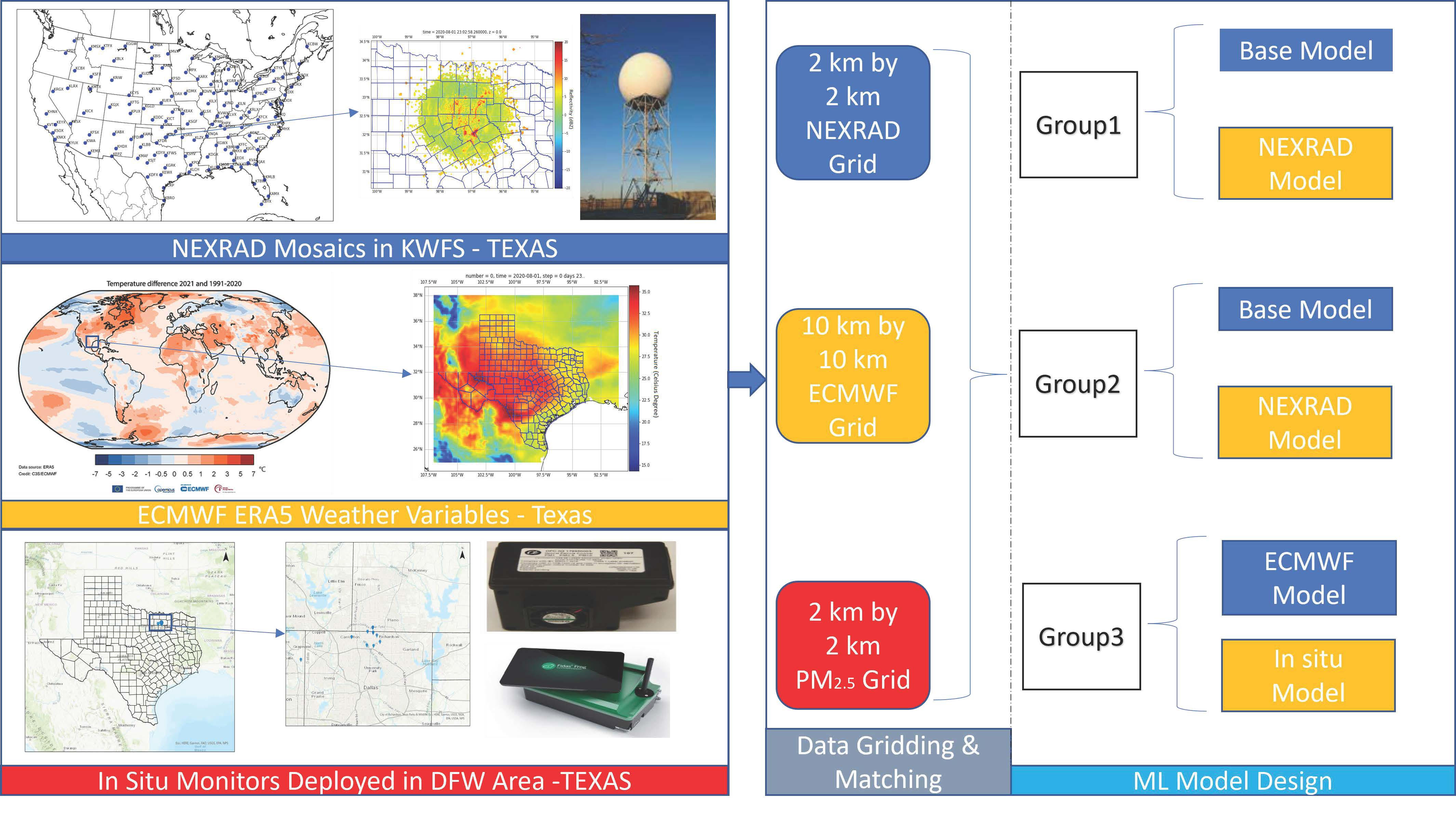
NEXRAD scans the atmosphere continuously by completing volume coverage patterns (VCP). Each VCP file contains data from only one radar station at a given timestamp, and the radar makes multiple 360-degree scans of the atmosphere, sampling at increasing elevation angles. A total of 160 NEXRAD sites operate independently across the country and Figure 1 shows the locations of these sites. KFWS is the NEXRAD station that covers the 31 PM sensors deployed in Dallas area. The VCP file from the KFWS station is converted to grid files every 15 min. Each day 96 NEXRAD grid files are generated covering monitoring sensors, and 3 years historical grid files are generated for the study area from July 2019 to June 2021. Grid files comprise vertically composed data from the ground up to one-kilometer elevation and have a spatial resolution of 2 km by 2 km. The variables include reflectivity, velocity, spectrum width, differential phase, differential reflectivity and cross correlation ratio. As the training dataset for machine learning models, these variables will be synchronized with PM values from the deployed sensors, meteorological data from ECMWF, and AOD from GOES-16. KFWS provides raw NEXRAD scan files every 10 min, which are interpolated and saved as netCDF files with a spatial resolution of 2 km. Interpolated files include ground to 1 km elevation composite values of the six variables. A total of six composite value surfaces could be extracted from one interpolated file.
2.2.2. High Temporal Resolution Monitoring Sites
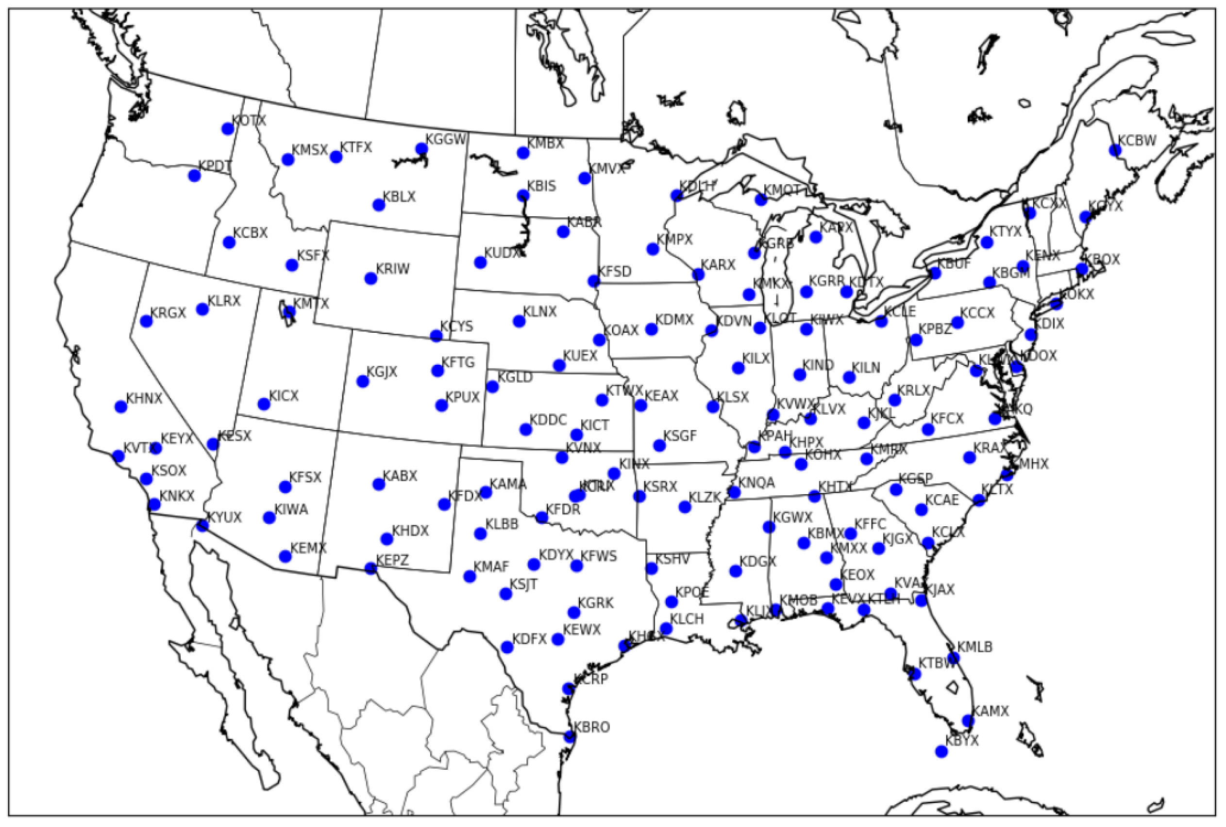
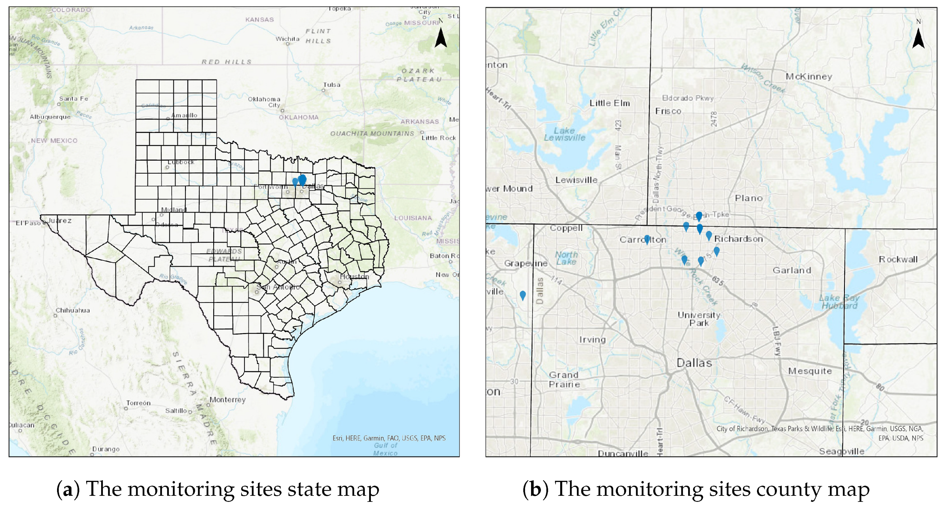
A total of 31 monitoring sites have been deployed in Dallas county, Collin county, and Tarrant county (See Figure 2). Most of them are located near the campus of University of Texas at Dallas in Richardson, and the rest are located in Fort Worth, Carrollton, and Plano respectively. Each site is equipped with two types of sensors, the Fidas Frog which is for PM concentration measuring, and the BME280 which is for weather condition monitoring. They are both cheap and inaccuracy. Thus, the calibration based on high-quality sensor ALPHA OPCN2 and AIRMAR [50] are required before these data are used for modeling. Upon calibration, these sensors can provide ground-level PM data as well as weather conditions measurements including humidity, temperature, pressure, and dew point temperature in 3 seconds interval, which have comparable quality to the expensive reference sensors. In this study, more than 10 million raw PM observations are collected between July 2019 and June 2021. After data aggregation and cleaning, these observations are then used to explore the application potential of NEXRAD in high temporal PM modeling.
2.2.3. ECMWF Grid
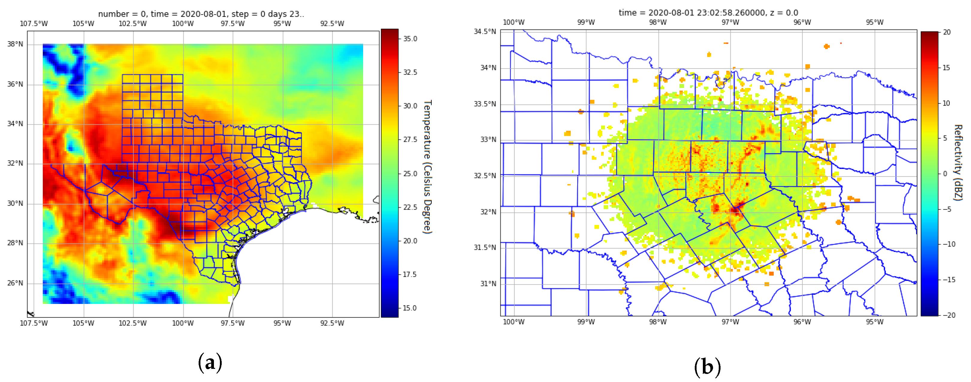
The ECMWF climate data store contains ERA5 land reanalysis hourly data back to 1979. A reanalysis combines model data with observations from across the world into a globally complete and consistent dataset using data assimilation. During this process, a previous forecast is combined with newly available observations in an optimal way to produce a new best estimate. This assimilation system can estimate data at locations where data coverage is low. For the purpose of model comparison, the four meteorological parameters that are simultaneously available from deployed sensors and ECMWF have been selected for PM modeling including humidity, ground temperature, dew point, and surface pressure. EAR5 gridded files are in the GRIB format, with a horizontal resolution of 0.1 degrees and hourly temporal resolution at a global level. A GRIB file is a format for storing and transporting gridded meteorological data. In this study, historical gridded EAR5 data are collected from July 2019 to June 2021, which will be synchronized with PM observations. Figure 3a is an example displaying the temperature and Figure 3b displays the reflectivity from NEXRAD.
2.2.4. GOES-16
Geostationary Operational Environmental Satellite (GOES)-R is the latest geostationary weather satellite of NOAA launched on 19 November 2016, which is equipped with the Advanced Baseline Imager (ABI) and 16 spectral bands [51]. GOES-R became GOES-16 when it reached geostationary orbit at 75.2 degrees west longitude. Over the North and South American continents, it provides high-temporal remote sensing data. The ABI offers four modes of operation, including Full Disk, Mesoscale, Continental US, and Flex. Data products generated by different ABI modes have different coverage scopes and spatial-temporal resolutions. Among these modes, the Continental US is the best mode since it scans the continent every 5 min with a spatial resolution of 0.5 km to 2 km. The AOD product retrieved from the continental US mode with a 5 min temporal resolution and 2 km spatial resolution is a valuable source that allows satellite-based PM modeling with an unparalleled temporal resolution. The raw GOES-16 AOD is available in NetCDF format on Amazon S3 and has its own fixed grid projection, which should be converted before being used for PM modeling.
2.2.5. Data Matching
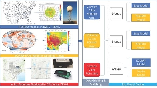
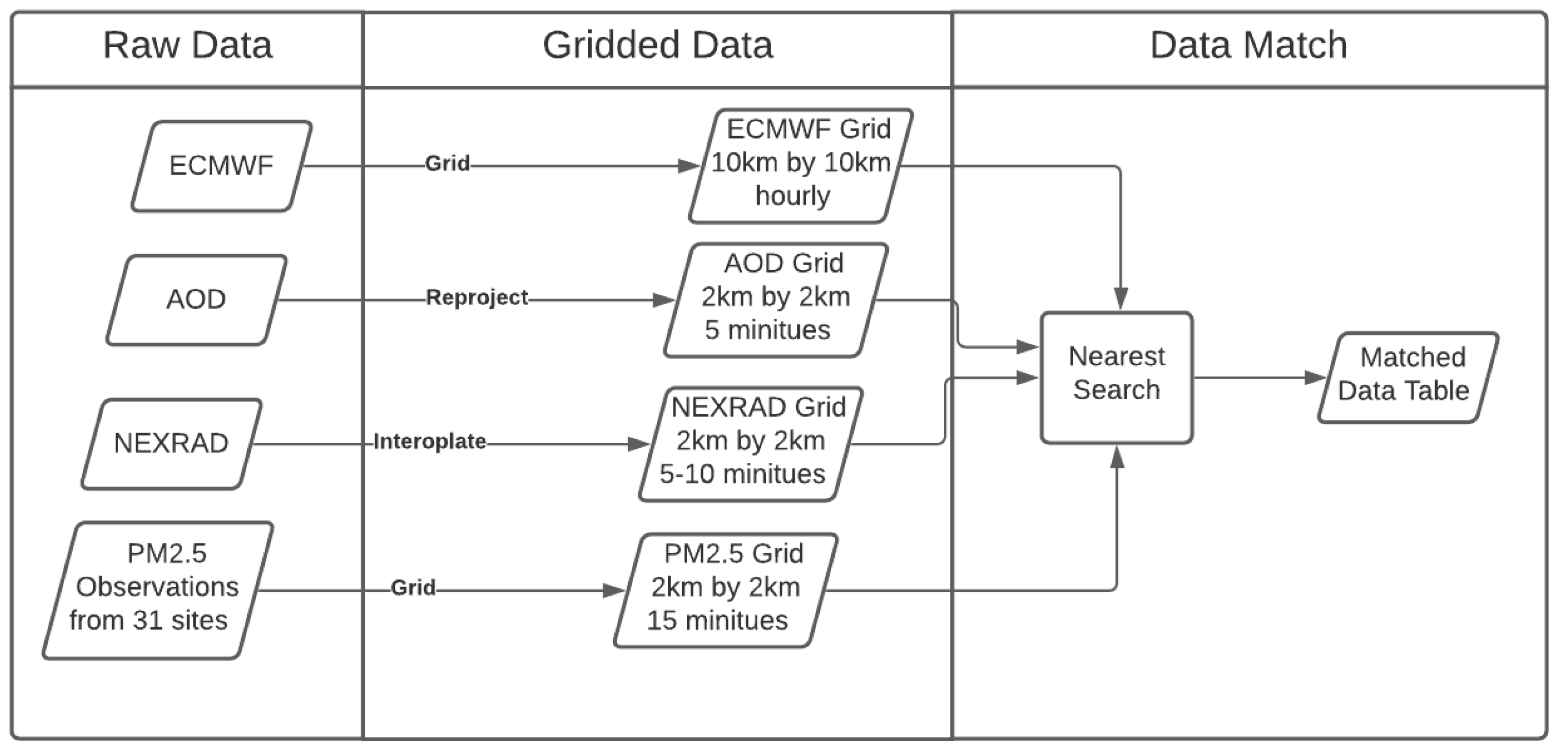
Figure 4 displays the four stages in the workflow including raw data processing, data gridding, and data matching. The ground observations from the 31 sensors, the meteorological data from ECMWF, the weather condition parameters from NEXRAD, and the AOD from GOES-16 are collected at different time stamps and in different formats. It is necessary to align these datasets into a consistent timetable for model training. The coordinates and timestamp information of each 2 km-by-2 km ground PM cell are retrieved. These coordinates and timestamp values are then used as query parameters to obtain meteorological and AOD variables from gridded NEXRAD, ECMWF, and GOES-16 files. These retrieved values are then attached to each of the PM ground observation cells. During the matching process, there are always grid pixels from NEXRAD and ECMWF that don’t perfectly match with the PM observations. A nearest search method is adopted in this case. In the time domain, ECMWF is recorded hourly while NEXRAD, PM, and AOD are recorded at an interval of less than 15 min. More specifically, the ECMWF file with the timestamp that is closest to the PM observation timestamp is selected as the candidate layer to match with the PM observation. In the spatial domain, ECMWF cells are in 10 km-by-10 km resolution while the NEXRAD, PM and AOD cells are in 2 km-by-2 km resolution. Hence, a perfect coordinate match between ECMWF and other gridded data is a rare case. In practice, a nearest search method is used to match values between these data sources by setting a distance tolerance threshold. In this study, tolerance is set as the ECMWF file’s spatial resolution. Once the matching process is done, a timetable containing PM observation values, meteorological factors, AOD, and weather condition parameters are generated. GOES-16 AOD is only available during the day to ensure data quality, and NEXRAD is only recording reflected signals that are strong enough to be detected. Thus, there are many empty AOD and NEXRAD values matched, and these observations will be removed from the data table.
2.3. Experiment Design
In this study, four models with different predictor variables are trained and evaluated. Three comparison groups are constructed by selecting two from the four models. For each comparison group, one model functions as the base model to benchmark the other model. Table 1 summarizes the four models with different predictor variables, and Table 2 summarizes the comparison groups.
As in Table 2, the first experiment group includes two models which both utilize weather variables from sensors, but one with NEXRAD and the other without NEXRAD. This group explores whether combining NEXRAD with in situ weather observations could improve the accuracy of PM modeling. Since sensor-measured weather variables have little meaning for PM estimation at locations without monitoring sensors, the adoption of ECMWF as a weather source is a more common practice in studies. Hence, the second experiment group includes two models that use ECMWF as their weather condition source, but one with NEXRAD and one without NEXRAD. In the third experiment group, sensor-measured weather variables are replaced by similar measurements from the ECMWF, and NEXRAD are not included for both models. This experiment group explores the impact on modeling accuracy by using ECMWF as an alternative weather source for in situ observations.
2.4. Machine Learning Approach
Data used in this study is vast in size, fast in generation, and complex in type which poses challenges for traditional data processing approaches. Under this circumstance, machine learning approach is adopted in this research. Machine learning is able to learn from samples and improve the prediction result automatically as more training samples are given. The feature of learning from samples makes machine learning an effective approach to reveal patterns and extract knowledge hidden behind Big Data. Machine learning is especially suitable for solving problems lacking the theoretical relationship between predictor variables and response variables. The use of machine learning in this study builds on our heritage of using machine learning for sensing applications over the last two decades [27,43,47,50,52,53,54,55,56].
The various resolutions and sources of the predictor variables may introduce noises into the training data set during the data gridding and data matching stages. A ensemble machine learning approach, which aggregates multiple weak learners into one model, is employed in this study to address this problem. The aggregation process of multiple weak learners could reduce the bias and variances. More specifically, the Classification and Regression Tree (CART) implementation of a decision tree is selected as the base learner for the ensemble model because of its high implementation efficiency, ease of interpretation, and low overfitting risk. The Gini index and twoing criteria are used for CART on feature selection optimization. Another important part of a machine learning model is hyperparameters, which act as tuning knobs. Any adjustments on these knobs can lead to different modeling results. The three main hyperparameter optimization methods are grid search, random search, and Bayesian optimization. In comparison to grid search and random search, Bayesian optimization can learn from previous optimization results and thus propose candidate searching spaces, which skips the step of defining each hyperparameter sample in advance and reduces computing time. A Bayesian hyperparameter optimization will be used to determine the ensemble method, the minimum sample size to split, maximum leaf nodes, and number of trees in this study.
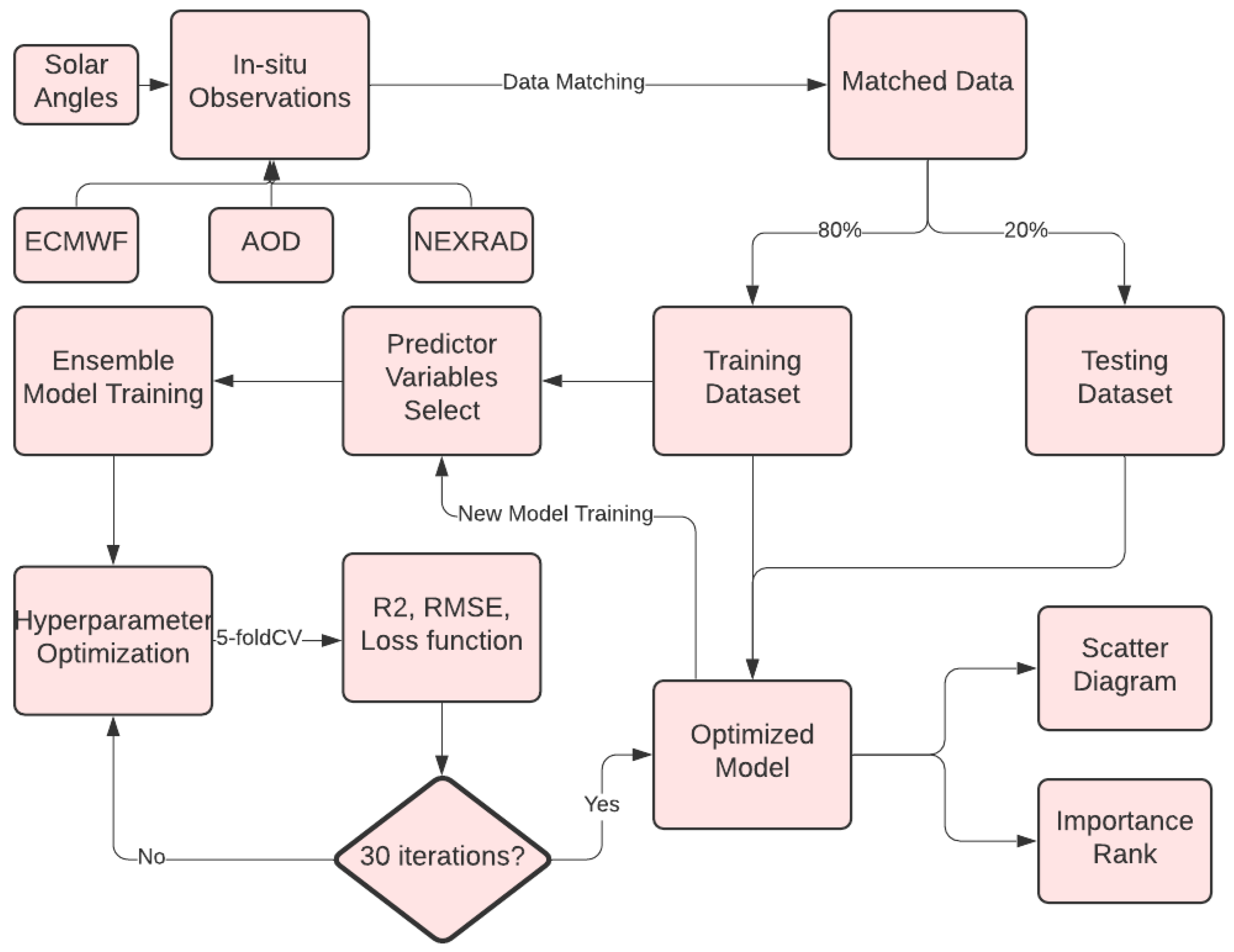
The whole dataset is divided into a training group and a testing group at a ratio of 80-20. The 5-fold cross-validation sampling technique is used to evaluate the model for the training set. The training set has been divided into five groups. One group is held out for evaluation, and the remaining four groups are used for model training. The model performance is summarized after five iterations. A further evaluation of the model is needed on the portion of testing to which it has never been exposed. Figure 5 illustrates the model training and validation process as a workflow.
3. Results
3.1. 5-Fold Cross-Validation Optimization
A Bayesian hyperparameter optimization process is utilized to discover the optimal hyperparameter settings for the four models, with 30 evaluation iterations. For each iteration, 5-fold cross validation technique is employed to measure the error through the objective function value, which is defined in the Equation (1):
where, cvloss is the average of the mean square error (MSE) summarized from 5-fold cross validation results.
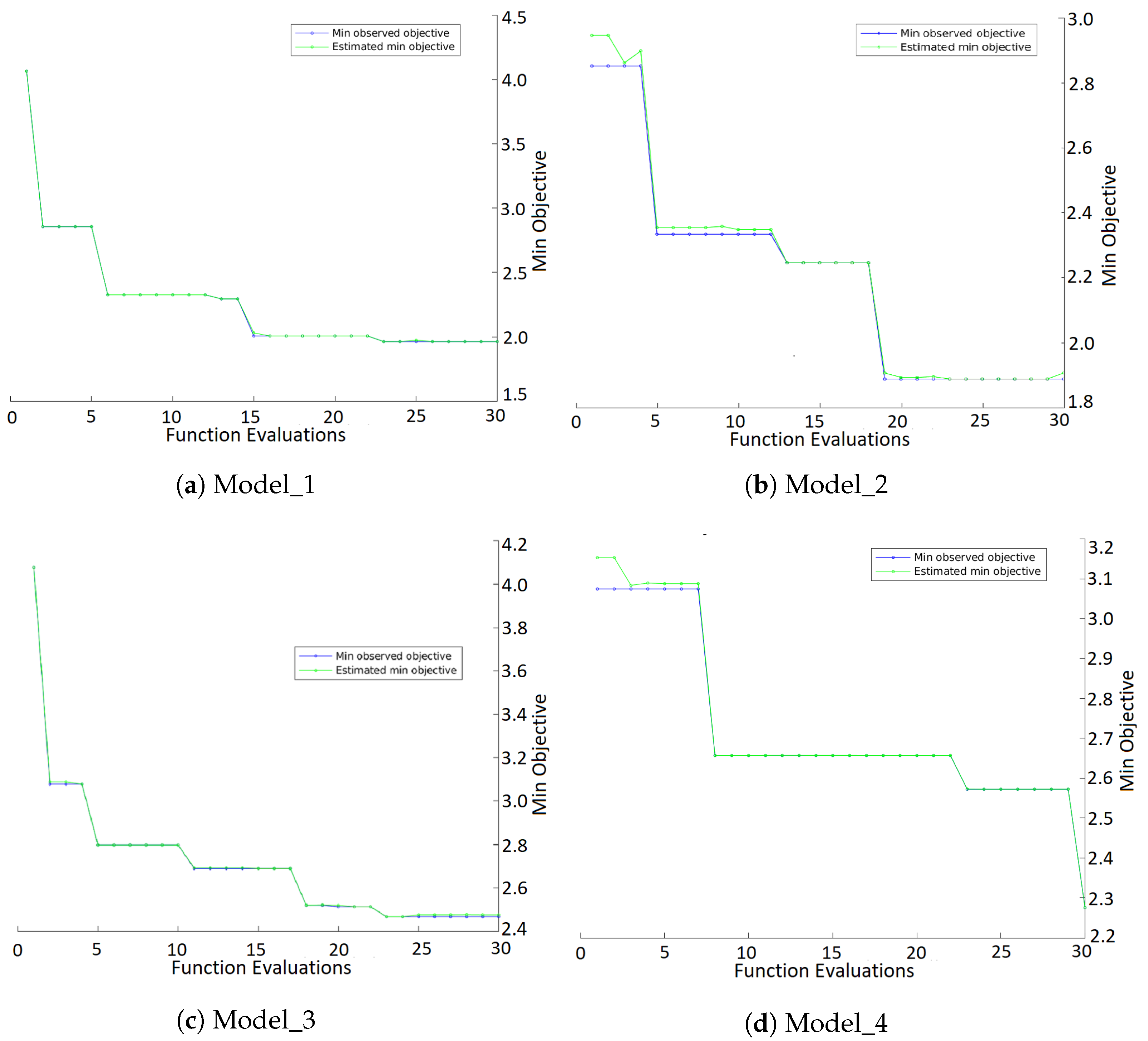
Figure 6 shows the best objective function value achieved at each iteration for the four models listed in Figure 1. The x-axis represents the number of optimization iterations, and the y-axis represents the objective function value. The blue line shows the current minimum objective function value observed, and the green line shows the estimated minimum objective function value. As in the figure, with increasing iterations, the objective function values improve. The minimum objective function values become stable after 15th, 19th, and 23th iterations for model_1, model_2, and model_3 respectively. For model_4, the best objective function value is achieved at the 30th iteration. The hyperparameters associated with the best objective function scores, as well as the R and the RMSE from 5-fold cross-validations for the four models are summarized in Table 3. Based on the 5-fold cross-validation results, the Model_2 has the best performance and the Model_3 has the worst performance.
3.2. Model Validation on Training and Testing Dataset
Once the Bayesian optimization process is complete, the four optimized models are then applied to the training and testing dataset for validation. Table 4 summarized the R and RMSE on the entire training and testing dataset. Need to mention that the R in Table 3 are summarized based on the 5 fold cross-validation during the hyperparameter optimization process, while the training R and the testing R in Table 4 are summarized from the training dataset and testing dataset.
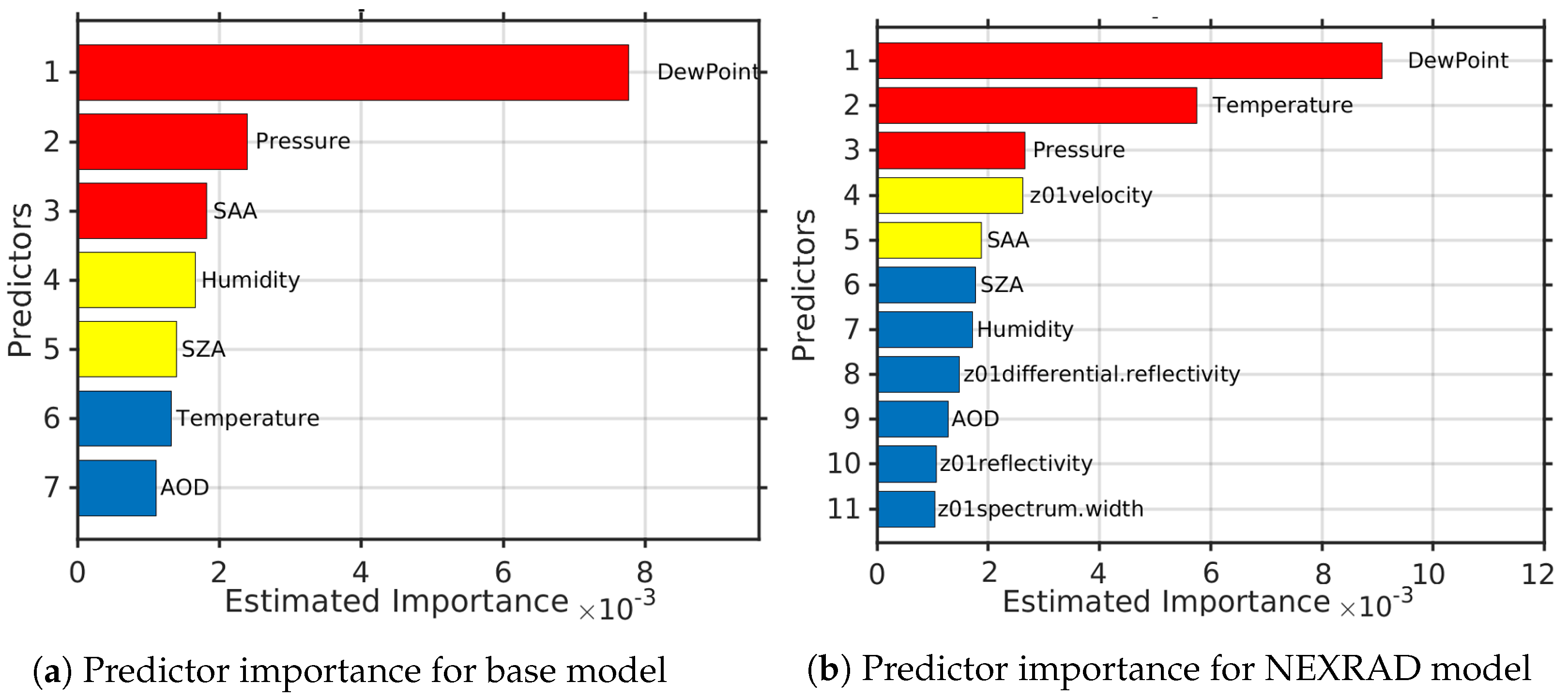
Tree-based ensemble machine learning models have the advantage of being able to track the contributions of each predictor to the model. During of process of node splitting, the variables with more power to decrease the impurity value gain more importance than those with less power. A scatter plot showing the influence of each predictor variable on the optimized ensemble model, and an importance rank plot is generated for each model in the following three comparison groups.
3.3. Comparison Group 1: NEXRAD Sensitive Analysis with In Situ Weather Variables
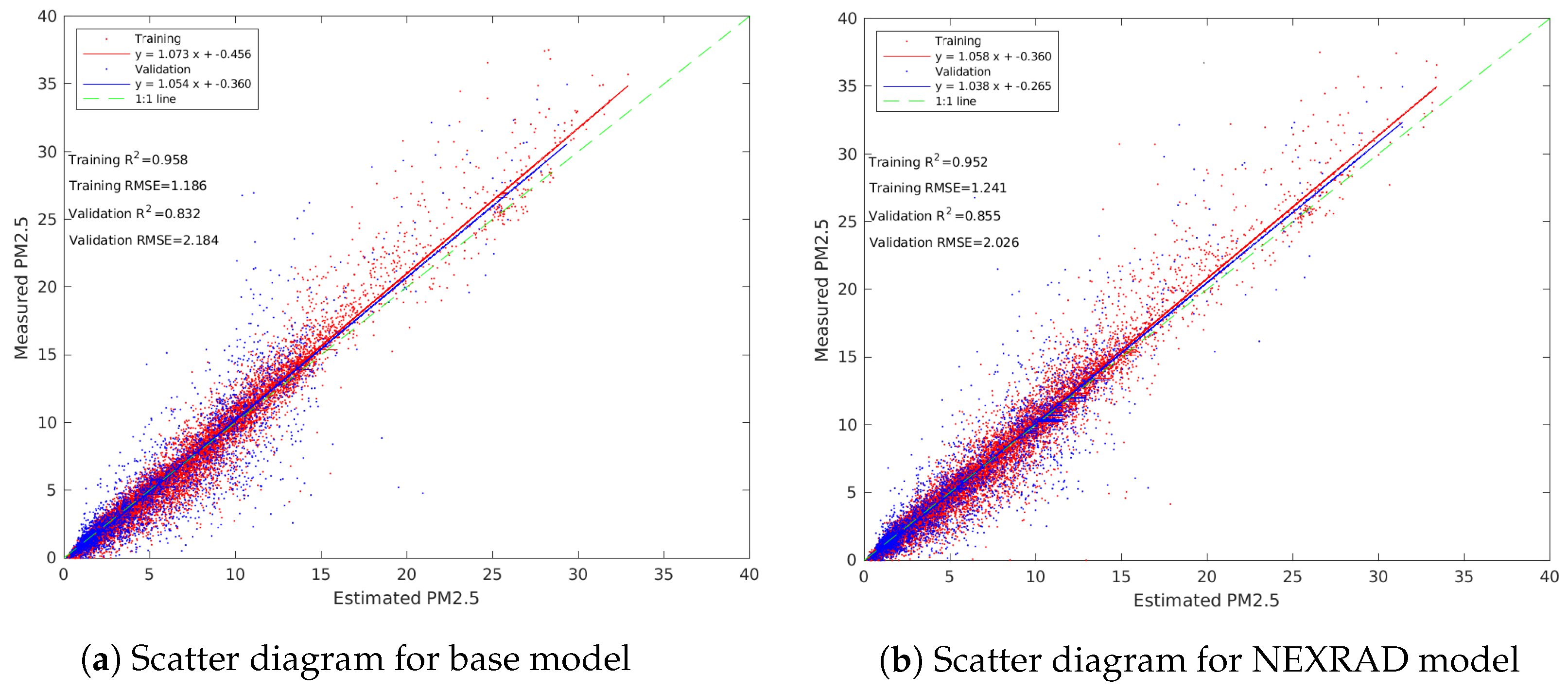
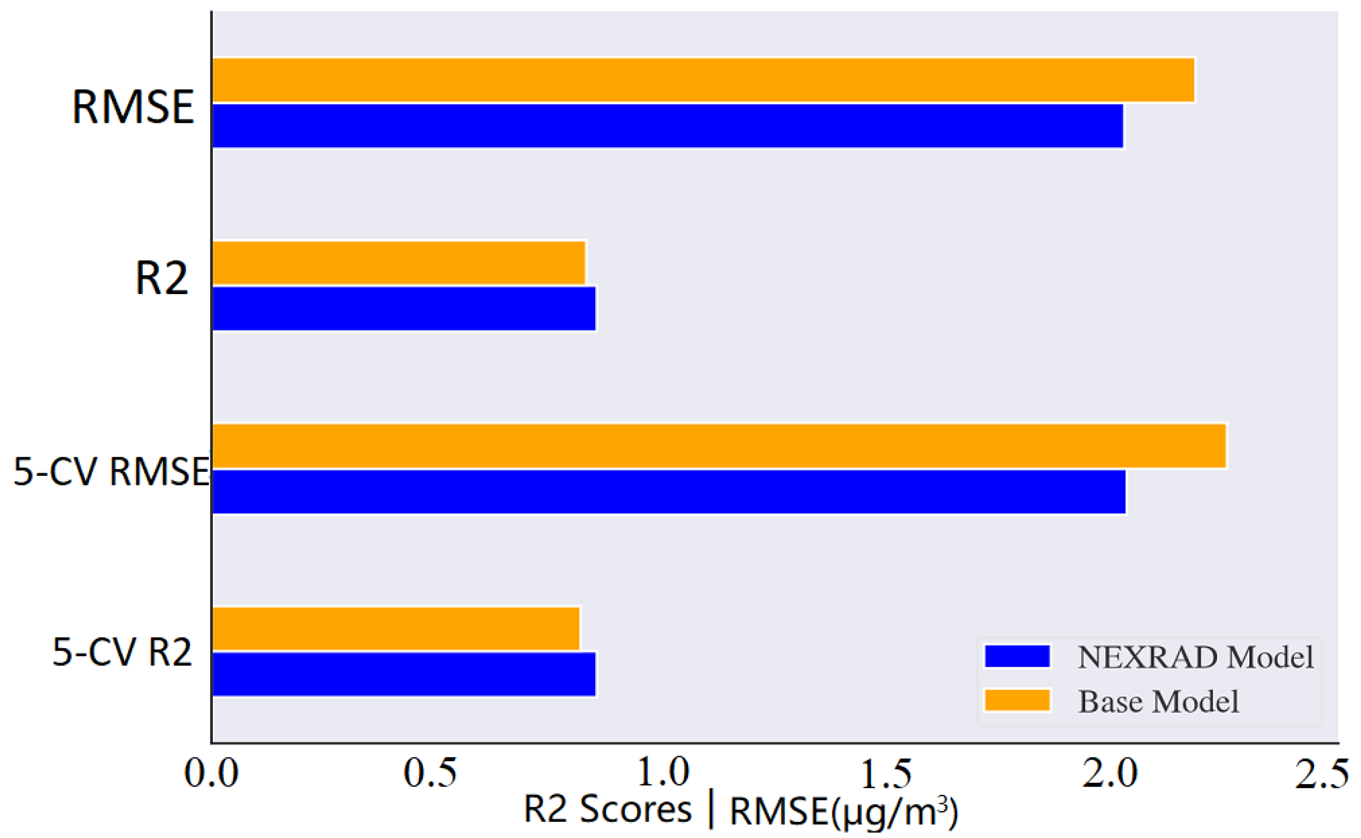
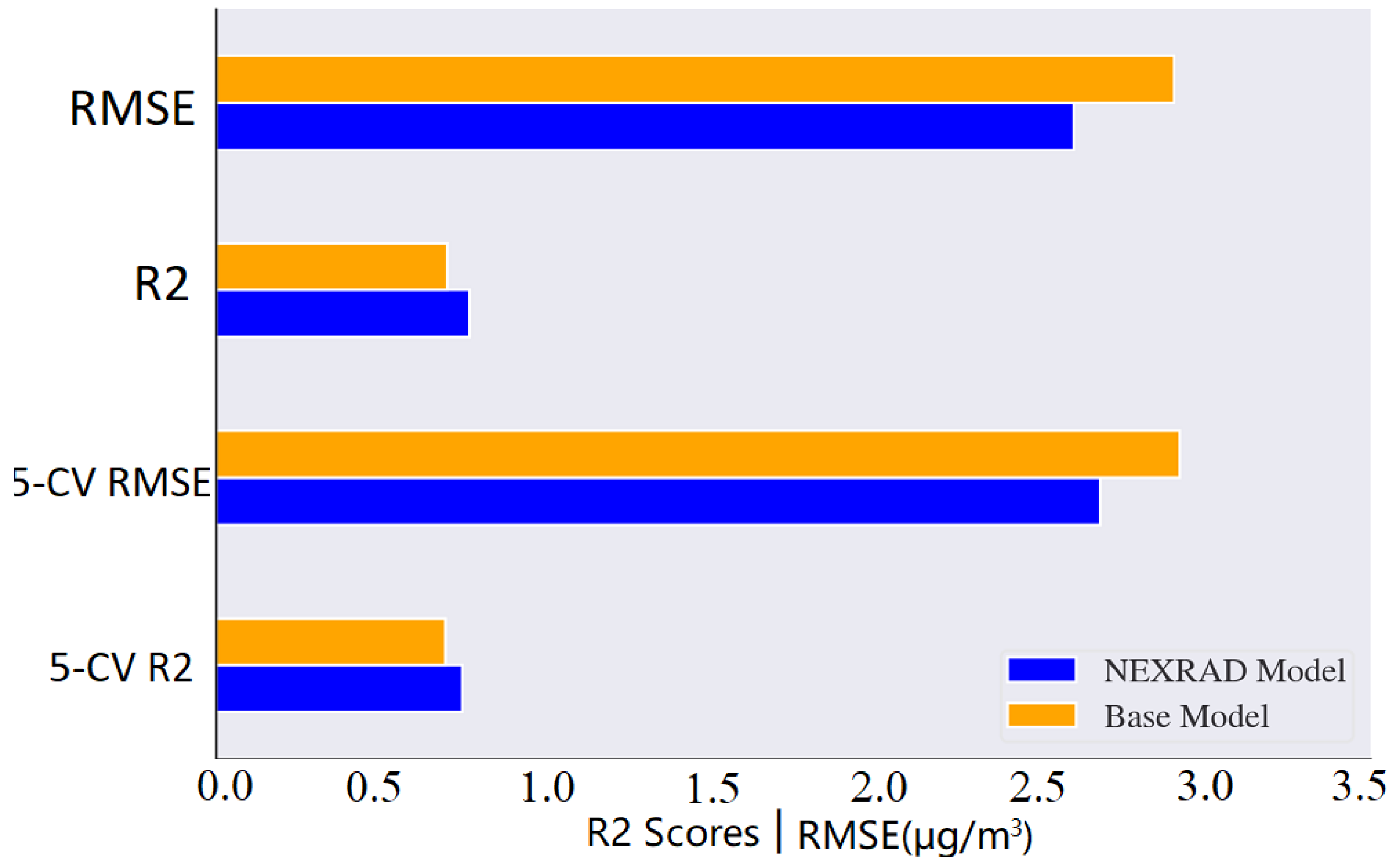
Comparison group 1 explores whether the combining of NEXRAD with in situ observed weather conditions could improve the PM modeling accuracy. The model_1 without radar and the model_2 with radar are included in this comparison group. For the convenience of comparison, the alias names “base model” and “NEXRAD model” are used for model_1 and model_2 respectively. In Figure 7, predicted values are plotted against measurement values for the base model and NEXRAD model. The training R and RMSE are calculated from the training which accounts for 80% of the whole dataset while the testing R and RMSE are calculated from the testing dataset that accounts for 20% of the whole dataset. These performance metrics correspond to the values in Table 4. Figure 8 compares model performances metrics side by side in a bar plot. These performance metrics correspond to the values in Table 3.
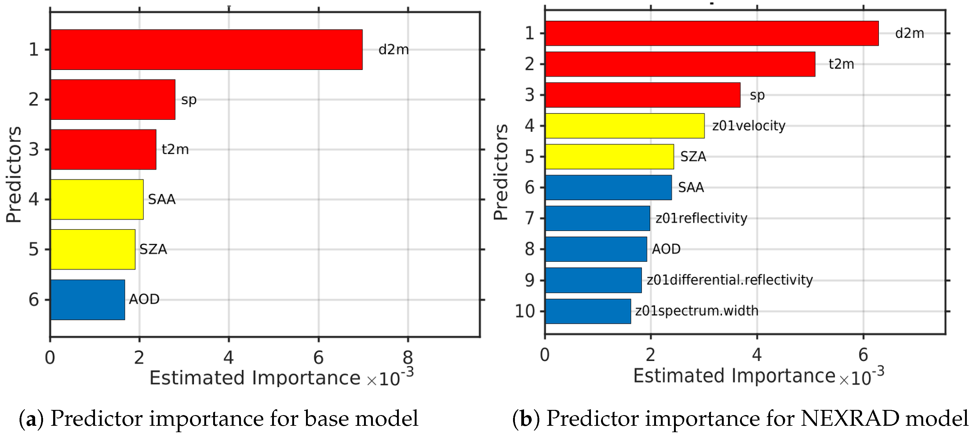
As in the scatter plots and bar plots, the NEXRAD model consistently shows higher R values and lower RMSE values than the base model on the testing dataset and cross-validation holdout dataset. Figure 9a displays the importance rank for the base model and NEXRAD model. The red and yellow bars represent the top five important predictor variables and the blue bar represents the remaining variables. According to this plot, the dew point temperature, pressure, humidity, and solar angles are the top five important predictor variables for the base model. In the Figure 9b, the dew point temperature, temperature, pressure, radar velocity, and solar azimuth angle are the top five important predictor variables for the NEXRAD model. Compared to the base model, velocity from NEXRAD contributes significantly to the performance of the NEXRAD model. The description of variables is listed in the Table 5.
3.4. Comparison Group 2: NEXRAD Sensitivity Analysis with ECMWF Weather Variables
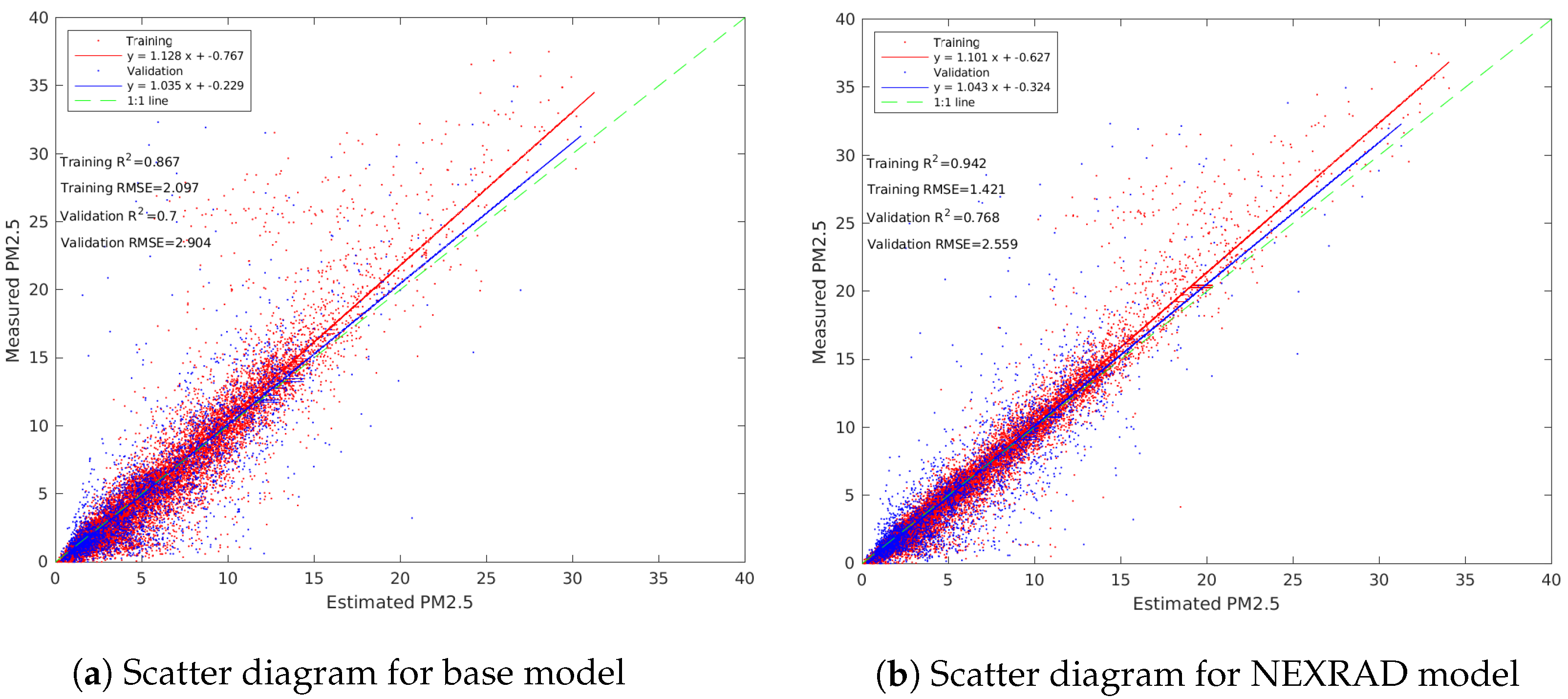
In situ weather condition observations, AOD, and the variables from NEXRAD have been explored for PM modeling in comparison group 1. Although the in situ weather condition variables are important predictors, they are only available at sites with sensors deployed, which limits the application potential for PM estimation. In comparison group 2, these in situ weather observations are replaced with the similar measurements from ECMWF for PM modeling, which provide continuous spatial coverage for PM modeling. This comparison group includes the model_3 and model_4, both of which use weather variables from ECMWF but one with radar and the other without radar. The alias “base model” and “NEXRAD model” are used for model_3 and model_4 (see Table 4) respectively in this comparison group. The scatter diagram, bar plot, and importance rank plot are generated in Figure 10, Figure 11 and Figure 12 respectively.
In the scatter plot (Figure 10), the NEXRAD model has better performance than the base model in terms of R and RMSE on both training and testing datasets. In the bar plot (Figure 11), the NEXRAD model has higher R and lower RMSE compared to the base model on testing data and 5 cross-validation holdout datasets. Compared to the model accuracy improvements from NEXRAD in group 1, the NEXRAD model in group 2 has more significant accuracy improvements. As in the Figure 12, the dew point temperature, surface pressure, temperature, and solar angles are the most important predictor variables for the base model. After adding the variables from NEXRAD, the radar velocity becomes the fourth important factor for the NEXRAD model.
3.5. Comparison Group 3: Weather Variables Sensitivity Analysis
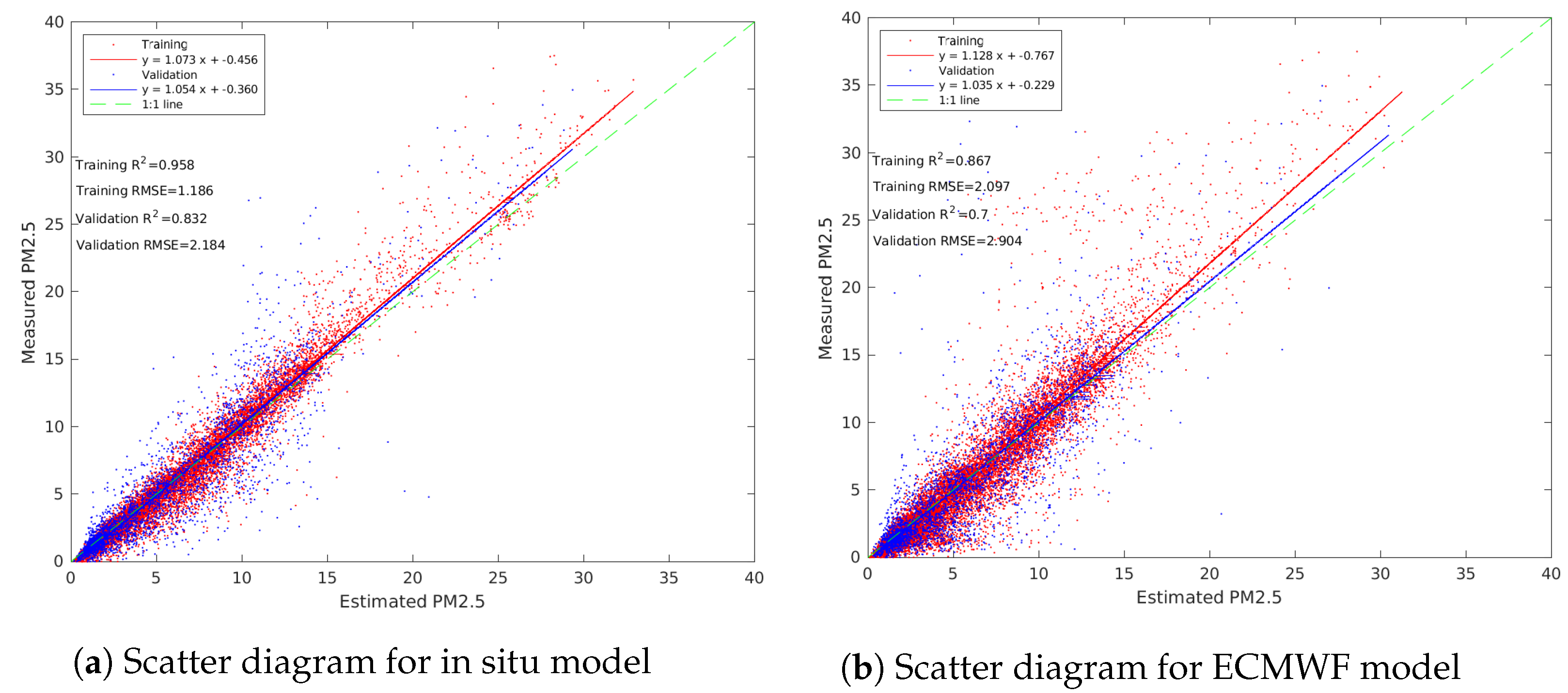
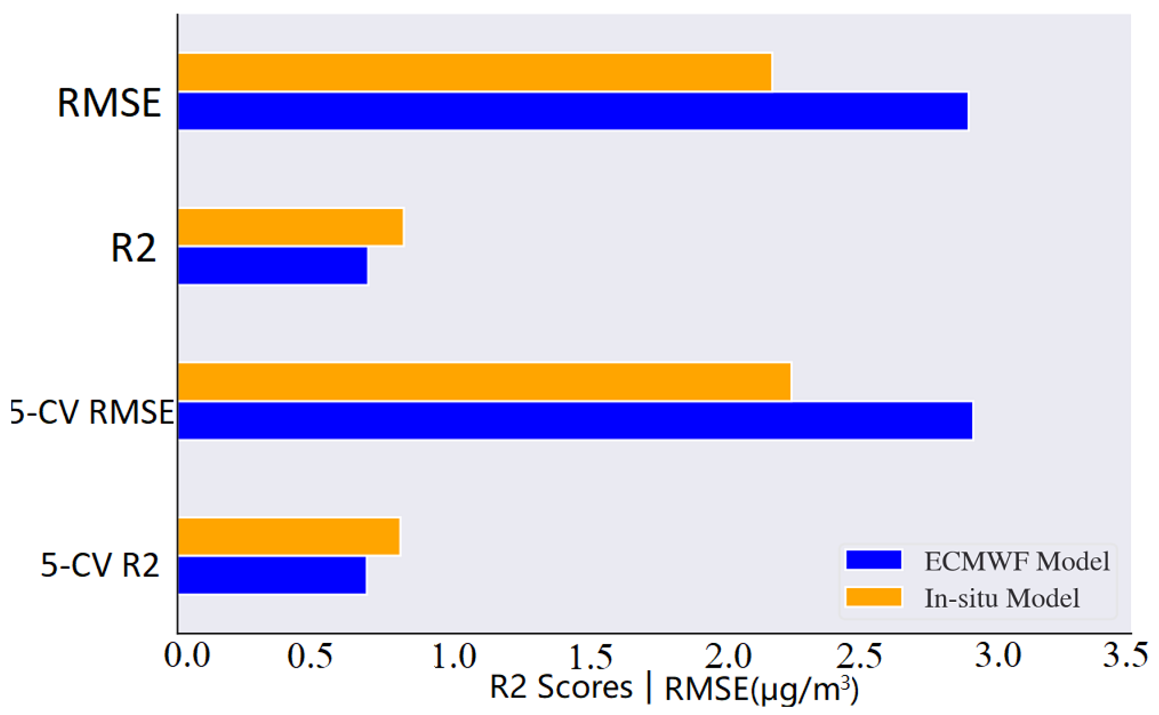
The weather variables from ECMWF provide continuous spatial coverage for PM modeling and estimation, but at the cost of a coarser temporal (hourly) and spatial (10 km) resolution. To investigate the model performances by replacing in situ weather observations with ECMWF products, model_1 and model_3 are compared in this group. For the convenience of comparison, the alias of “in situ model” and “ECMWF model” are used for model_1 and model_3 respectively, neither of which includes NEXRAD. The scatter diagram, bar plot, and importance rank plot for the third comparison group are in the Figure 13, Figure 14 and Figure 15 respectively.
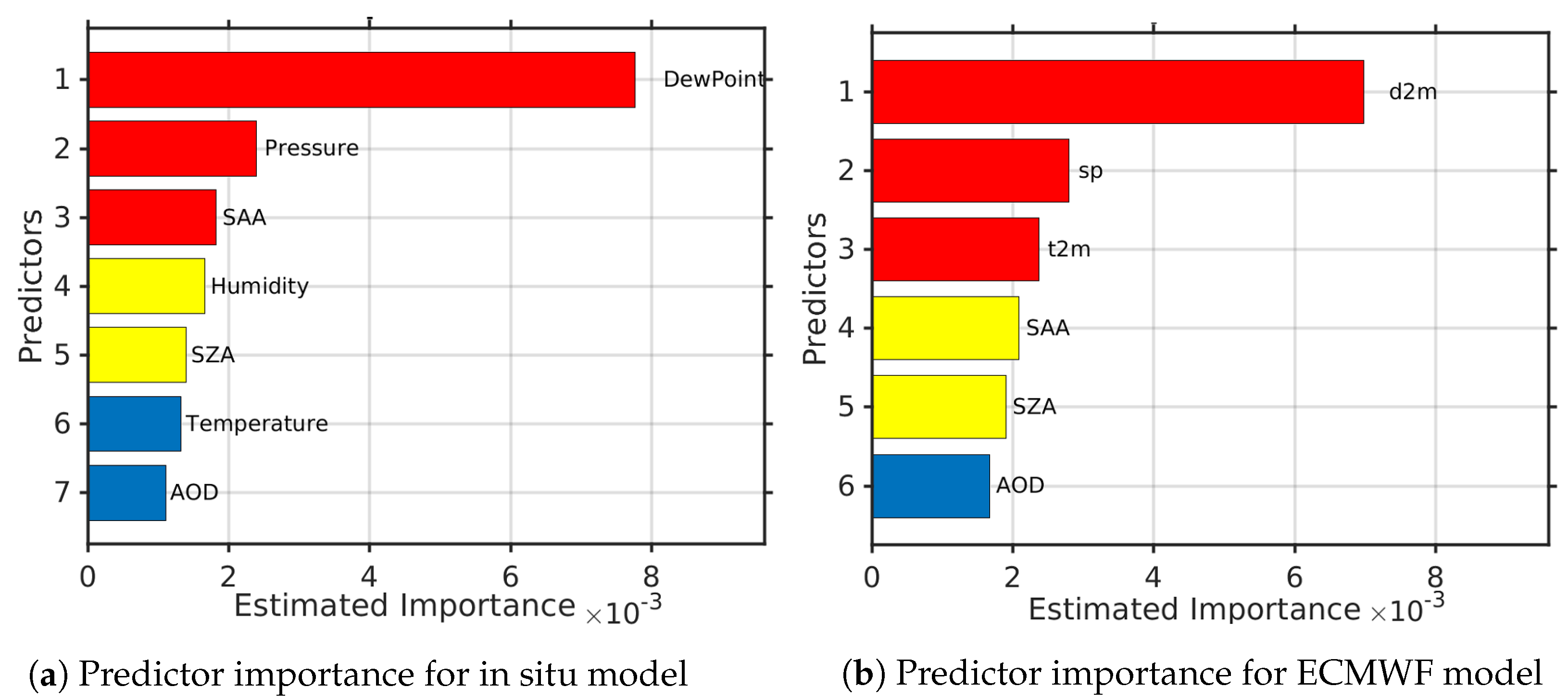
According to the Figure 13, the R value drops 0.13 and the RMSE increases 0.72 on the testing dataset by replacing the in situ weather variables with ECMWF variables. Although with the performance drop, the model with ECMWF still achieves satisfactory results with a 0.7 R score and 2.9 RMSE on the testing dataset. Figure 14 shows the results from the testing data which are consistent with results from the 5-fold cross-validation results. In Figure 15, the dew point temperature and surface pressures are the two most important predictor variables for both models.
4. Discussion
The wind influences the PM concentration during saltation. Particles are carried by the wind and move in their own way as they creep, saltate, or suspend. When particles moved by the wind collide with each other or with the ground surface, the saltation process occurs. Researchers have found that wind plays an important role in saltation, in which fine size airborne particulates including PM and PM can be emitted [57,58]. A NEXRAD’s spectrum width and velocity can provide information on how fast and what is the direction the wind is moving. Hence, variables from NEXRAD are incorporated together with in situ observation and ECMWF variables for PM modeling in this study. The performances of models with and without NEXRAD are compared in group 1 (see Table 6). Limited by the availability of in situ weather observations, the variables from ECMWF are widely adopted as an alternative source for measuring weather conditions, which are commonly used for meteorological studies and PM estimations [34,59]. Therefore, group 2 replaces in situ observations with similar variables from ECMWF to investigate the model performances with and without NEXRAD. Replacing in situ observations with similar variables from ECMWF allows better spatial coverage, but at the cost of lower spatial and temporal resolution, and higher uncertainties. Under this circumstance, the comparison group 3 explores how effective the variables from ECMWF are in PM modeling compared to the sensor measured in situ weather observations.
A summary of the model comparison results can be found in Table 6. The results from group 1 and group 2 demonstrate that variables from NEXRAD could provide extra weather information, especially the velocity, which helps to improve the PM modeling accuracy. The more significant model accuracy improvement in group 2 compared to group 1 encourages us to believe that when lacking in situ weather observations, NEXRAD can serve as an important supplementary information source to ECMWF for a better PM modeling accuracy. Group 3 shows that although ECMWF could serve as an alternative weather variables source for in situ weather observations in PM modeling and has better spatial coverage, variables from ECMWF are at hourly intervals, while the other variables are available every 15 min. As a result, variables from ECMWF need to be interpolated to match the temporal resolution of the rest variables for PM modeling, which could introduce noise and lead to a model accuracy drop.
In addition to NEXRAD, ECMWF, and in situ observations, variables from GOES-16 and solar angles (see Table 5) are employed as predictor variables as well. Previous studies examined the relationship between AOD and PM concentration varies depending on the time of day [60]. Solar angles are closely related to the local time and have a huge influence on the AOD quality, which provides important information to help the PM estimation. This conforms with the Figure 9, Figure 12 and Figure 15, where the variables from solar angles contribute significantly to PM modeling accuracy.
5. Conclusions
By comparing the four established models in three groups, this study has made the following discovery. First, the in situ weather observations including humidity, temperature, dew point, and pressure, together with AOD from GOES-16 and solar angles could achieve good modeling results (0.83 R) for PM concentrations at a 15 min temporal resolution. Second, combining variables from NEXRAD with an in situ model could improve the R modeling accuracy by 2.8%. Third, combining variables from NEXRAD with ECMWF could achieve more accuracy improvements (9.7%) compared to the accuracy improvements from the in situ models. Last, by replacing in situ observations with variables from ECMWF, the model has an 0.7 R score on the testing dataset, which is 0.13 less than the model with in situ weather observation.
Several novel facts have been uncovered by these discoveries that could provide insights for future research. Due to NEXRAD’s high scanning frequency, even though it cannot detect PM particles directly, it can provide supplementary weather conditions that improve PM modeling, especially for high temporal PM modeling. In addition, due to the incompatibility in resolution and veracity issues, using weather variables from ECMWF as an alternative for in situ observation leads to a significant model accuracy drop. However, when in situ observations are not available, weather variables from ECMWF are still an effective source for PM modeling. Furthermore, NEXRAD improves model accuracy more significantly in the model based on variables from ECMWF than in the model based on variables from in situ observations. These facts suggest that NEXRAD can be utilized as a supplementary weather source for high temporal PM modeling, especially in the absence of in situ weather measurements.
Author Contributions
Conceptualization, X.Y. and D.J.L.; methodology, X.Y. and D.J.L.; software, X.Y. and C.S.S.; validation, X.Y.; formal analysis, X.Y.; investigation, X.Y.; resources, X.Y., C.S.S. and D.J.L.; data curation, X.Y. and L.O.H.W.; writing—original draft preparation, X.Y.; writing—review and editing, D.J.L.; visualization, X.Y. and C.S.S.; supervision, D.J.L.; project administration, X.Y. and D.J.L.; funding acquisition, D.J.L. and C.S.S. All authors have read and agreed to the published version of the manuscript.
Funding
This research was funded by National Science Foundation CNS Division of Computer and Network Systems grant 1541227, and EPA Grant Number 83996501. The APC was funded by C.S.S.
Institutional Review Board Statement
Not applicable.
Informed Consent Statement
Not applicable.
Data Availability Statement
The Python code for NEXRAD data preparation is available at URL: https://github.com/xiaoheyu/NEXRAD (accessed on 10 January 2022).
Acknowledgments
Christopher Simmons is gratefully acknowledged for his computational support. The authors acknowledge the Texas Research and Education Cyberinfrastructure Services (TRECIS) Center, NSF Award #2019135, and the University of Texas at Dallas for providing HPC, visualization, database, or grid resources and support that have contributed to the research results reported within this paper. URL: https://trecis.cyberinfrastructure.org/ (accessed on 28 October 2021). The authors acknowledge the Texas Advanced Computing Center (TACC) at the University of Texas at Austin for providing HPC, visualization, database, or grid resources that have contributed to the research results reported within this paper. URL: http://www.tacc.utexas.edu (accessed on 28 October 2021). This research received support from USAMRMC Award Number W81XWH-18-1-0400. National Science Foundation CNS Division of Computer and Network Systems grant 1541227, and EPA Grant Number 83996501.
Conflicts of Interest
The authors declare no conflict of interest.
References
- Boucher, O. Atmospheric aerosols. In Atmospheric Aerosols; Springer: Berlin/Heidelberg, Germany, 2015; pp. 9–24. [Google Scholar]
- Pope, C.A., III; Dockery, D.W. Health effects of fine particulate air pollution: Lines that connect. J. Air Waste Manag. Assoc. 2006, 56, 709–742. [Google Scholar] [CrossRef]
- Hua, J.; Yin, Y.; Peng, L.; Du, L.; Geng, F.; Zhu, L. Acute effects of black carbon and PM2.5 on children asthma admissions: A time-series study in a Chinese city. Sci. Total Environ. 2014, 481, 433–438. [Google Scholar] [CrossRef]
- Lim, S.S.; Vos, T.; Flaxman, A.D.; Danaei, G.; Shibuya, K.; Adair-Rohani, H.; AlMazroa, M.A.; Amann, M.; Anderson, H.R.; Andrews, K.G.; et al. A comparative risk assessment of burden of disease and injury attributable to 67 risk factors and risk factor clusters in 21 regions, 1990–2010: A systematic analysis for the Global Burden of Disease Study 2010. Lancet 2012, 380, 2224–2260. [Google Scholar] [CrossRef] [Green Version]
- Yu, W.; Liu, S.; Jiang, J.; Chen, G.; Luo, H.; Fu, Y.; Xie, L.; Li, B.; Li, N.; Chen, S.; et al. Burden of ischemic heart disease and stroke attributable to exposure to atmospheric PM2.5 in Hubei province, China. Atmos. Environ. 2020, 221, 117079. [Google Scholar] [CrossRef]
- Bartell, S.M.; Longhurst, J.; Tjoa, T.; Sioutas, C.; Delfino, R.J. Particulate air pollution, ambulatory heart rate variability, and cardiac arrhythmia in retirement community residents with coronary artery disease. Environ. Health Perspect. 2013, 121, 1135–1141. [Google Scholar] [CrossRef]
- Lary, M.A.; Allsopp, L.; Lary, D.J.; Sterling, D.A. Using machine learning to examine the relationship between asthma and absenteeism. Environ. Monit. Assess. 2019, 191, 332. [Google Scholar] [CrossRef]
- Clark, N.M.; Brown, R.; Joseph, C.L.; Anderson, E.W.; Liu, M.; Valerio, M.A. Effects of a comprehensive school-based asthma program on symptoms, parent management, grades, and absenteeism. Chest 2004, 125, 1674–1679. [Google Scholar] [CrossRef]
- Tsakiris, A.; Iordanidou, M.; Paraskakis, E.; Tsalkidis, A.; Rigas, A.; Zimeras, S.; Katsardis, C.; Chatzimichael, A. The presence of asthma, the use of inhaled steroids, and parental education level affect school performance in children. BioMed. Res. Int. 2013, 2013, 762805. [Google Scholar] [CrossRef] [Green Version]
- Pope, C.A., III; Burnett, R.T.; Thun, M.J.; Calle, E.E.; Krewski, D.; Ito, K.; Thurston, G.D. Lung cancer, cardiopulmonary mortality, and long-term exposure to fine particulate air pollution. JAMA 2002, 287, 1132–1141. [Google Scholar] [CrossRef] [Green Version]
- Zang, Z.; Li, D.; Guo, Y.; Shi, W.; Yan, X. Superior PM2.5 Estimation by Integrating Aerosol Fine Mode Data from the Himawari-8 Satellite in Deep and Classical Machine Learning Models. Remote Sens. 2021, 13, 2779. [Google Scholar] [CrossRef]
- Liu, J.; Weng, F.; Li, Z.; Cribb, M.C. Hourly PM2.5 estimates from a geostationary satellite based on an ensemble learning algorithm and their spatiotemporal patterns over central east China. Remote Sens. 2019, 11, 2120. [Google Scholar] [CrossRef] [Green Version]
- Engel-Cox, J.A.; Hoff, R.M.; Haymet, A. Recommendations on the use of satellite remote-sensing data for urban air quality. J. Air Waste Manag. Assoc. 2004, 54, 1360–1371. [Google Scholar] [CrossRef] [PubMed]
- Hoff, R.M.; Christopher, S.A. Remote sensing of particulate pollution from space: Have we reached the promised land? J. Air Waste Manag. Assoc. 2009, 59, 645–675. [Google Scholar] [CrossRef]
- Song, W.; Jia, H.; Huang, J.; Zhang, Y. A satellite-based geographically weighted regression model for regional PM2.5 estimation over the Pearl River Delta region in China. Remote Sens. Environ. 2014, 154, 1–7. [Google Scholar] [CrossRef]
- Zheng, C.; Zhao, C.; Zhu, Y.; Wang, Y.; Shi, X.; Wu, X.; Chen, T.; Wu, F.; Qiu, Y. Analysis of influential factors for the relationship between PM_ (2.5) and AOD in Beijing. Atmos. Chem. Phys. 2017, 17, 13473–13489. [Google Scholar] [CrossRef] [Green Version]
- Zhang, H.; Hoff, R.M.; Engel-Cox, J.A. The relation between Moderate Resolution Imaging Spectroradiometer (MODIS) aerosol optical depth and PM2.5 over the United States: A geographical comparison by US Environmental Protection Agency regions. J. Air Waste Manag. Assoc. 2009, 59, 1358–1369. [Google Scholar] [CrossRef] [Green Version]
- Yang, Q.; Yuan, Q.; Yue, L.; Li, T.; Shen, H.; Zhang, L. The relationships between PM2.5 and aerosol optical depth (AOD) in mainland China: About and behind the spatio-temporal variations. Environ. Pollut. 2019, 248, 526–535. [Google Scholar] [CrossRef]
- Wu, J.; Yao, F.; Li, W.; Si, M. VIIRS-based remote sensing estimation of ground-level PM2.5 concentrations in Beijing–Tianjin–Hebei: A spatiotemporal statistical model. Remote Sens. Environ. 2016, 184, 316–328. [Google Scholar] [CrossRef]
- Kondragunta, S.; Laszlo, I.; Ciren, P.; Zhang, H.; Liu, H.; Huang, J.; Huff, A. Exceptional events monitoring using S-NPP VIIRS aerosol products. In Proceedings of the 2017 IEEE International Geoscience and Remote Sensing Symposium (IGARSS), Fort Worth, TX, USA, 23–28 July 2017; pp. 1285–1287. [Google Scholar]
- Jung, C.R.; Chen, W.T.; Nakayama, S.F. A National-Scale 1-km Resolution PM2.5 Estimation Model over Japan Using MAIAC AOD and a Two-Stage Random Forest Model. Remote Sens. 2021, 13, 3657. [Google Scholar] [CrossRef]
- Yu, X.; Lary, D.J.; Simmons, C.S. PM2.5 Modeling and Historical Reconstruction over the Continental USA Utilizing GOES-16 AOD. Remote Sens. 2021, 13, 4788. [Google Scholar] [CrossRef]
- Liu, Y.; Vu, B.N.; Bi, J.; Kondragunta, S.; Zhang, H. Characterizing PM2.5 during the 2018 California wildfire season using GOES-16 data. In Proceedings of the AGU Fall Meeting Abstracts, San Francisco, CA, USA, 9–13 December 2019; Volume 2019, p. A51F-02. [Google Scholar]
- Zhang, H.; Kondragunta, S.; Laszlo, I. Surface PM2.5 Estimates from GOES and VIIRS AOD over the United States. In Proceedings of the AGU Fall Meeting Abstracts, Washington, DC, USA, 10–14 December 2018; Volume 2018, p. A51G-2238. [Google Scholar]
- Vu, B.; Bi, J.; Liu, Y. GOES16-Based Estimation of Hourly PM2.5 Levels during the Camp Fire Wildfire Episode in California. In Proceedings of the ISEE Conference Abstracts, Virtual Meeting, 24–27 August 2020; Volume 2020. [Google Scholar]
- Bai, H.; Zheng, Z.; Zhang, Y.; Huang, H.; Wang, L. Comparison of satellite-based PM2.5 estimation from aerosol optical depth and top-of-atmosphere reflectance. Aerosol Air Qual. Res. 2021, 21, 200257. [Google Scholar] [CrossRef]
- Lary, D.J.; Faruque, F.S.; Malakar, N.; Moore, A.; Roscoe, B.; Adams, Z.L.; Eggelston, Y. Estimating the global abundance of ground level presence of particulate matter (PM2.5). Geospat. Health 2014, 8, S611–S630. [Google Scholar] [CrossRef]
- Sathe, Y.; Kulkarni, S.; Gupta, P.; Kaginalkar, A.; Islam, S.; Gargava, P. Application of Moderate Resolution Imaging Spectroradiometer (MODIS) Aerosol Optical Depth (AOD) and Weather Research Forecasting (WRF) model meteorological data for assessment of fine particulate matter (PM2.5) over India. Atmos. Pollut. Res. 2019, 10, 418–434. [Google Scholar] [CrossRef]
- Lu, D.; Xu, J.; Yang, D.; Zhao, J. Spatio-temporal variation and influence factors of PM2.5 concentrations in China from 1998 to 2014. Atmos. Pollut. Res. 2017, 8, 1151–1159. [Google Scholar] [CrossRef]
- Zhao, X.; Zhou, W.; Han, L.; Locke, D. Spatiotemporal variation in PM2.5 concentrations and their relationship with socioeconomic factors in China’s major cities. Environ. Int. 2019, 133, 105145. [Google Scholar] [CrossRef]
- Eeftens, M.; Beelen, R.; De Hoogh, K.; Bellander, T.; Cesaroni, G.; Cirach, M.; Declercq, C.; Dedele, A.; Dons, E.; De Nazelle, A.; et al. Development of land use regression models for PM2.5, PM2.5 absorbance, PM10 and PMcoarse in 20 European study areas; results of the ESCAPE project. Environ. Sci. Technol. 2012, 46, 11195–11205. [Google Scholar] [CrossRef]
- Liu, Y.; Paciorek, C.J.; Koutrakis, P. Estimating regional spatial and temporal variability of PM2.5 concentrations using satellite data, meteorology, and land use information. Environ. Health Perspect. 2009, 117, 886–892. [Google Scholar] [CrossRef] [Green Version]
- Alvarez, H.B.; Echeverria, R.S.; Alvarez, P.S.; Krupa, S. Air quality standards for particulate matter (PM) at high altitude cities. Environ. Pollut. 2013, 173, 255–256. [Google Scholar] [CrossRef]
- Schneider, R.; Vicedo-Cabrera, A.M.; Sera, F.; Masselot, P.; Stafoggia, M.; de Hoogh, K.; Kloog, I.; Reis, S.; Vieno, M.; Gasparrini, A. A satellite-based spatio-temporal machine learning model to reconstruct daily PM2.5 concentrations across Great Britain. Remote Sens. 2020, 12, 3803. [Google Scholar] [CrossRef] [PubMed]
- Lin, Y.C.; Chi, W.J.; Lin, Y.Q. The improvement of spatial-temporal resolution of PM2.5 estimation based on micro-air quality sensors by using data fusion technique. Environ. Int. 2020, 134, 105305. [Google Scholar] [CrossRef]
- ECMWF. ECMWF. 2020. Available online: https://www.ecmwf.int/en/about/what-we-do (accessed on 10 January 2022).
- Molina, M.O.; Gutiérrez, C.; Sánchez, E. Comparison of ERA5 surface wind speed climatologies over Europe with observations from the HadISD dataset. Int. J. Climatol. 2021, 41, 4864–4878. [Google Scholar] [CrossRef]
- Taszarek, M.; Pilguj, N.; Allen, J.T.; Gensini, V.; Brooks, H.E.; Szuster, P. Comparison of convective parameters derived from ERA5 and MERRA-2 with Rawinsonde data over Europe and North America. J. Clim. 2021, 34, 3211–3237. [Google Scholar]
- Shikhovtsev, A.Y.; Kovadlo, P.; Kiselev, A. Astroclimatic statistics at the Sayan solar observatory. Sol.-Terr. Phys. 2020, 6, 102–107. [Google Scholar]
- Saltikoff, E.; Friedrich, K.; Soderholm, J.; Lengfeld, K.; Nelson, B.; Becker, A.; Hollmann, R.; Urban, B.; Heistermann, M.; Tassone, C. An overview of using weather radar for climatological studies: Successes, challenges, and potential. Bull. Am. Meteorol. Soc. 2019, 100, 1739–1752. [Google Scholar] [CrossRef]
- Chilson, C.; Avery, K.; McGovern, A.; Bridge, E.; Sheldon, D.; Kelly, J. Automated detection of bird roosts using NEXRAD radar data and Convolutional Neural Networks. Remote Sens. Ecol. Conserv. 2019, 5, 20–32. [Google Scholar] [CrossRef]
- Wang, Y.; Pu, Z. Assimilation of Radial Velocity from Coastal NEXRAD into HWRF for Improved Forecasts of Landfalling Hurricanes. Weather Forecast. 2021, 36, 587–599. [Google Scholar] [CrossRef]
- Zewdie, G.K.; Lary, D.J.; Liu, X.; Wu, D.; Levetin, E. Estimating the daily pollen concentration in the atmosphere using machine learning and NEXRAD weather radar data. Environ. Monit. Assess. 2019, 191, 418. [Google Scholar] [CrossRef]
- Hufford, G.L.; Kelley, H.L.; Sparkman, W.; Moore, R.K. Use of real-time multisatellite and radar data to support forest fire management. Weather Forecast. 1998, 13, 592–605. [Google Scholar] [CrossRef]
- Geng, G.; Zhang, Q.; Martin, R.V.; van Donkelaar, A.; Huo, H.; Che, H.; Lin, J.; He, K. Estimating long-term PM2.5 concentrations in China using satellite-based aerosol optical depth and a chemical transport model. Remote Sens. Environ. 2015, 166, 262–270. [Google Scholar] [CrossRef]
- Lv, B.; Hu, Y.; Chang, H.H.; Russell, A.G.; Cai, J.; Xu, B.; Bai, Y. Daily estimation of ground-level PM2.5 concentrations at 4 km resolution over Beijing-Tianjin-Hebei by fusing MODIS AOD and ground observations. Sci. Total Environ. 2017, 580, 235–244. [Google Scholar] [CrossRef]
- Lary, D.; Lary, T.; Sattler, B. Using machine learning to estimate global PM2.5 for environmental health studies. Environ. Health Insights 2015, 9, EHI-S15664. [Google Scholar] [CrossRef]
- Wu, D.; Lary, D.J.; Zewdie, G.K.; Liu, X. Using machine learning to understand the temporal morphology of the PM 2.5 annual cycle in East Asia. Environ. Monit. Assess. 2019, 191, 272. [Google Scholar] [CrossRef]
- Liu, X.; Wu, D.; Zewdie, G.K.; Wijerante, L.; Timms, C.I.; Riley, A.; Levetin, E.; Lary, D.J. Using machine learning to estimate atmospheric Ambrosia pollen concentrations in Tulsa, OK. Environ. Health Insights 2017, 11, 1178630217699399. [Google Scholar] [CrossRef] [Green Version]
- Wijeratne, L.O.; Kiv, D.R.; Aker, A.R.; Talebi, S.; Lary, D.J. Using Machine Learning for the Calibration of Airborne Particulate Sensors. Sensors 2020, 20, 99. [Google Scholar] [CrossRef] [Green Version]
- NASA. GOES16. 2021. Available online: https://www.goes-r.gov/mission/history.html (accessed on 10 January 2022).
- Yu, X.; Lary, D.J. Cloud Detection Using an Ensemble of Pixel-Based Machine Learning Models Incorporating Unsupervised Classification. Remote Sens. 2021, 13, 3289. [Google Scholar] [CrossRef]
- Lary, D.J.; Remer, L.; MacNeill, D.; Roscoe, B.; Paradise, S. Machine learning and bias correction of MODIS aerosol optical depth. IEEE Geosci. Remote Sens. Lett. 2009, 6, 694–698. [Google Scholar] [CrossRef] [Green Version]
- Lary, D.J. Artificial Intelligence in Geoscience and Remote Sensing; INTECH Open Access Publisher: London, UK, 2010. [Google Scholar]
- Zewdie, G.K.; Lary, D.J.; Levetin, E.; Garuma, G.F. Applying deep neural networks and ensemble machine learning methods to forecast airborne ambrosia pollen. Int. J. Environ. Res. Public Health 2019, 16, 1992. [Google Scholar] [CrossRef] [PubMed] [Green Version]
- Lary, D.J.; Schaefer, D.; Waczak, J.; Aker, A.; Barbosa, A.; Wijeratne, L.O.; Talebi, S.; Fernando, B.; Sadler, J.; Lary, T.; et al. Autonomous Learning of New Environments with a Robotic Team Employing Hyper-Spectral Remote Sensing, Comprehensive In-Situ Sensing and Machine Learning. Sensors 2021, 21, 2240. [Google Scholar] [CrossRef] [PubMed]
- Tatarko, J.; Kucharski, M.; Li, H.; Li, H. PM2.5 and PM10 emissions by breakage during saltation of agricultural soils. Soil Tillage Res. 2021, 208, 104902. [Google Scholar] [CrossRef]
- Borlina, C.S.; Rennó, N.O. The impact of a severe drought on dust lifting in California’s Owens Lake Area. Sci. Rep. 2017, 7, 1784. [Google Scholar] [CrossRef] [PubMed]
- Wu, C.; Li, K.; Bai, K. Validation and Calibration of CAMS PM2.5 Forecasts Using In Situ PM2.5 Measurements in China and United States. Remote Sens. 2020, 12, 3813. [Google Scholar] [CrossRef]
- Ma, Z.; Hu, X.; Sayer, A.M.; Levy, R.; Zhang, Q.; Xue, Y.; Tong, S.; Bi, J.; Huang, L.; Liu, Y. Satellite-based spatiotemporal trends in PM2.5 concentrations: China, 2004–2013. Environ. Health Perspect. 2016, 124, 184–192. [Google Scholar] [CrossRef] [PubMed] [Green Version]
Figure 1.
The 160 NEXRAD monitoring stations across the United States.

Figure 2.
The maps show the locations of monitoring sites at the (a) state level and (b) county level in Dallas. In total, 31 monitoring sensors are deployed, and some of them are clustered in the pinpoints.
Figure 2.
The maps show the locations of monitoring sites at the (a) state level and (b) county level in Dallas. In total, 31 monitoring sensors are deployed, and some of them are clustered in the pinpoints.

Figure 3.
The example raster layers used for high temporal PM study. Figure (a) shows the temperature layer from ECMWF in 1 August 2020, and (b) shows the reflectivity layer from KFWS NEXRAD site in 1 August 2020.
Figure 3.
The example raster layers used for high temporal PM study. Figure (a) shows the temperature layer from ECMWF in 1 August 2020, and (b) shows the reflectivity layer from KFWS NEXRAD site in 1 August 2020.

Figure 4.
The flow chart presents the data pre-processing and data matching process.

Figure 5.
Flow chart illustrates the machine learning model training and validation process.

Figure 6.
The objective function evaluation results during the hyper-parameter optimization process. The red line represents the observed best objective function values at each iteration, and the blue line represents the estimated best function values at each iteration. (a) The Model_1 without NEXRAD, (b) the Model_2 with NEXRAD. (c) the Model_3 without NEXRAD, and (d) the Model_4 with NEXRAD.

Figure 7.
The scatter diagram for models on training data set and testing data set. Red dots represent the training observations and blue dots represent the validation observations. Red line and blue line are fitting lines for training points and validation points respectively. (a) shows the estimated PM against measured PM for base model, and the (b) displays the estimated PM against measured PM for NEXRAD model.

Figure 8.
The model performances comparison bar chart for group 1. The Y-axis displays model performance metric names and the X-axis shows the scores for both R and RMSE. The RMSE and the R of models are summarized on the testing dataset. The 5-CV RMSE and 5-CV R are summarized based on 5-fold cross-validation results on the training dataset. In this chart, the RMSE and R are compared between the NEXRAD Model and the Base Model.

Figure 9.
The importance rank plots for models with and without NEXRAD in comparison group 1. The top five important variables are in red and yellow, while the rest are in blue.
Figure 9.
The importance rank plots for models with and without NEXRAD in comparison group 1. The top five important variables are in red and yellow, while the rest are in blue.

Figure 10.
The scatter diagram for models with variables from ECMWF. (a)The base model without NEXRAD and (b) the NEXRAD model with NEXRAD.
Figure 10.
The scatter diagram for models with variables from ECMWF. (a)The base model without NEXRAD and (b) the NEXRAD model with NEXRAD.

Figure 11.
The model performances comparison bar chart for group 2. The meaning of X axis and Y axis is the same as in Figure 8. The RMSE and R are compared between the Base Model and NEXRAD Model.
Figure 11.
The model performances comparison bar chart for group 2. The meaning of X axis and Y axis is the same as in Figure 8. The RMSE and R are compared between the Base Model and NEXRAD Model.

Figure 12.
The importance rank plots for models with and without NEXRAD in comparison group 2. The description of variables is listed in the Table 5.
Figure 12.
The importance rank plots for models with and without NEXRAD in comparison group 2. The description of variables is listed in the Table 5.

Figure 13.
The scatter diagram for models with variables from ECMWF. (a) The in situ model with weather variables from in situ observations, and (b) the ECMWF model with weather variables from ECMWF.
Figure 13.
The scatter diagram for models with variables from ECMWF. (a) The in situ model with weather variables from in situ observations, and (b) the ECMWF model with weather variables from ECMWF.

Figure 14.
The model performances comparison bar chart for group 3. The meaning of X axis and Y axis is the same as in Figure 8. The RMSE and R are compared between the ECMWF Model and In-situ Model.
Figure 14.
The model performances comparison bar chart for group 3. The meaning of X axis and Y axis is the same as in Figure 8. The RMSE and R are compared between the ECMWF Model and In-situ Model.

Figure 15.
The importance rank plots for models using variables from in situ observation and variables from ECMWF in comparison group 3. The description of variables is listed in the Table 5.
Figure 15.
The importance rank plots for models using variables from in situ observation and variables from ECMWF in comparison group 3. The description of variables is listed in the Table 5.


Table 1.
The selected predictor variables for the 4 models.
| Model Name | In Situ Weather | ECMWF | NEXRAD | AOD | Solar Angles |
|---|---|---|---|---|---|
| Model_1 | ✓ | ✓ | ✓ | ||
| Model_2 | ✓ | ✓ | ✓ | ✓ | |
| Model_3 | ✓ | ✓ | ✓ | ||
| Model_4 | ✓ | ✓ | ✓ | ✓ |
Table 2.
The 3 comparison groups as well as the models included in each group.
| Comparison Group | Model Name | Weather Source | Design Purpose |
|---|---|---|---|
| Group 1 | Model_1 | Sensors | NEXRAD VS No NEXRAD |
| Model_2 | |||
| Group 2 | Model_3 | ECMWF | NEXRAD VS No NEXRAD |
| Model_4 | |||
| Group 3 | Model_1 | Sensors, ECMWF | in situ VS ECMWF |
| Model_3 |
Table 3.
The best 5-fold cross-validation optimization results for the four models as well as the optimized hyper-parameter settings.
Table 3.
The best 5-fold cross-validation optimization results for the four models as well as the optimized hyper-parameter settings.
| Model Name | Loss Function | R | RMSE | Method | Trees | Min Leaf Size | Max Splits | Variables to Sample | CPU Time |
|---|---|---|---|---|---|---|---|---|---|
| Model_1 | 1.963 | 0.82 | 2.253 | Bag | 39 | 1 | 11,450 | 4 | 2730 |
| Model_2 | 1.888 | 0.855 | 2.032 | Bag | 10 | 2 | 1969 | 8 | 1372 |
| Model_3 | 2.467 | 0.697 | 2.921 | Bag | 19 | 5 | 12,031 | 3 | 925 |
| Model_4 | 2.275 | 0.747 | 2.68 | Bag | 28 | 1 | 6298 | 10 | 1753 |
Table 4.
The optimized model performances on training and testing dataset.
| Model Name | Training R | Testing R | Training RMSE | Testing RMSE |
|---|---|---|---|---|
| Model_1 | 0.958 | 0.832 | 1.186 | 2.184 |
| Model_2 | 0.952 | 0.855 | 1.241 | 2.026 |
| Model_3 | 0.867 | 0.7 | 2.097 | 2.904 |
| Model_4 | 0.942 | 0.768 | 1.421 | 2.599 |
Table 5.
The predictor variables names as well as their source and description are listed.
| Source | Var Name | Description |
|---|---|---|
| ECMWF | d2m | Dewpoint temperature at 2 m |
| t2m | Temperature at 2 m | |
| sp | Surface pressure | |
| Sensors | dewpoint | Dewpoint temperature from sensor |
| temperature | Temperature from sensor | |
| pressure | Pressure from sensor | |
| humidity | Humidity from sensor | |
| NEXRAD | z01velocity | Wind speed of particles detected |
| z01reflectivity | Energy return to radar at ground level | |
| z01spectrum width | Distribution of velocities within a bin | |
| z01differential reflectivity | Horizontal to vertical power ratio | |
| GOES-16 | AOD | Aerosol Optical Depth |
| Solar Angles | SAA | Solar Azimuth Angle |
| SZA | Solar Zenith Angle |
Table 6.
Group comparison metrics. 5-CV R and 5-CV RMSE represent 5-fold cross-validation results from training dataset; R and RMSE represent the validation results from testing dataset.
Table 6.
Group comparison metrics. 5-CV R and 5-CV RMSE represent 5-fold cross-validation results from training dataset; R and RMSE represent the validation results from testing dataset.
| Groups | In Group Alias | 5-CV R | Difference | R | Difference | 5-CV RMSE | Difference | RMSE | Difference |
|---|---|---|---|---|---|---|---|---|---|
| Group 1 | Base Model | 0.820 | 0.035 | 0.832 | 0.023 | 2.253 | 0.221 | 2.184 | 0.158 |
| NEXRAD Model | 0.855 | 0.855 | 2.032 | 2.026 | |||||
| Group 2 | Base Model | 0.697 | 0.051 | 0.700 | 0.068 | 2.921 | 0.241 | 2.904 | 0.305 |
| NEXRAD Model | 0.747 | 0.768 | 2.680 | 2.599 | |||||
| Group 3 | in situ Model | 0.820 | 0.123 | 0.832 | 0.132 | 2.253 | 0.667 | 2.184 | 0.720 |
| ECMWF Model | 0.697 | 0.700 | 2.921 | 2.904 |
Publisher’s Note: MDPI stays neutral with regard to jurisdictional claims in published maps and institutional affiliations. |
© 2022 by the authors. Licensee MDPI, Basel, Switzerland. This article is an open access article distributed under the terms and conditions of the Creative Commons Attribution (CC BY) license (https://creativecommons.org/licenses/by/4.0/).
Share and Cite
MDPI and ACS Style
Yu, X.; Lary, D.J.; Simmons, C.S.; Wijeratne, L.O.H. High Spatial-Temporal PM2.5 Modeling Utilizing Next Generation Weather Radar (NEXRAD) as a Supplementary Weather Source. Remote Sens. 2022, 14, 495. https://doi.org/10.3390/rs14030495
AMA Style
Yu X, Lary DJ, Simmons CS, Wijeratne LOH. High Spatial-Temporal PM2.5 Modeling Utilizing Next Generation Weather Radar (NEXRAD) as a Supplementary Weather Source. Remote Sensing. 2022; 14(3):495. https://doi.org/10.3390/rs14030495
Chicago/Turabian StyleYu, Xiaohe, David J. Lary, Christopher S. Simmons, and Lakitha O. H. Wijeratne. 2022. "High Spatial-Temporal PM2.5 Modeling Utilizing Next Generation Weather Radar (NEXRAD) as a Supplementary Weather Source" Remote Sensing 14, no. 3: 495. https://doi.org/10.3390/rs14030495
Note that from the first issue of 2016, this journal uses article numbers instead of page numbers. See further details here.