
TCD-Net: A Novel Deep Learning Framework for Fully Polarimetric Change Detection Using Transfer Learning


1
School of Surveying and Geospatial Engineering, College of Engineering, University of Tehran, Tehran 14174-66191, Iran
2
C-CORE, 1 Morrissey Road, St. John’s, NL A1B 3X5, Canada
3
Department of Electrical and Computer Engineering, Memorial University of Newfoundland, St. John’s, NL A1C 5S7, Canada
*
Author to whom correspondence should be addressed.
Remote Sens. 2022, 14(3), 438; https://doi.org/10.3390/rs14030438
Submission received: 12 December 2021
/
Revised: 14 January 2022
/
Accepted: 17 January 2022
/
Published: 18 January 2022
(This article belongs to the Special Issue Synthetic Aperture Radar (SAR) Meets Deep Learning)
Abstract
:Due to anthropogenic and natural activities, the land surface continuously changes over time. The accurate and timely detection of changes is greatly important for environmental monitoring, resource management and planning activities. In this study, a novel deep learning-based change detection algorithm is proposed for bi-temporal polarimetric synthetic aperture radar (PolSAR) imagery using a transfer learning (TL) method. In particular, this method has been designed to automatically extract changes by applying three main steps as follows: (1) pre-processing, (2) parallel pseudo-label training sample generation based on a pre-trained model and fuzzy c-means (FCM) clustering algorithm, and (3) classification. Moreover, a new end-to-end three-channel deep neural network, called TCD-Net, has been introduced in this study. TCD-Net can learn more strong and abstract representations for the spatial information of a certain pixel. In addition, by adding an adaptive multi-scale shallow block and an adaptive multi-scale residual block to the TCD-Net architecture, this model with much lower parameters is sensitive to objects of various sizes. Experimental results on two Uninhabited Aerial Vehicle Synthetic Aperture Radar (UAVSAR) bi-temporal datasets demonstrated the effectiveness of the proposed algorithm compared to other well-known methods with an overall accuracy of 96.71% and a kappa coefficient of 0.82.
1. Introduction
The proliferation of remote sensing (RS) images at different temporal and spatial resolutions have increased its use in a wide range of global environmental and management applications, including change detection [1,2,3,4,5], target detection [6,7], wetland classification [8,9,10], oil spill detection [11,12,13], disaster monitoring [14,15] and so on. Detection of change is one of the most important applications of RS, which is essential for better resource management.
Change detection (CD) is the process of identifying changes, caused by manmade or natural factors, in multi-temporal Earth Observation (EO) data [16]. CD algorithms are commonly employed to monitor changes in different applications, including land use and land cover (LULC) [17,18], deforestation [19], urban development [20] and natural disaster [20].
In recent years, Synthetic Aperture Radar (SAR) sensors have become one of the most popular alternatives to other RS techniques because they can provide imaging in all weather conditions, day or night. In addition, SAR sensors are capable of penetrating through clouds, rain, smoke, snow, dust and so on. Therefore, these factors cannot affect the ability of SAR sensors. In addition, SAR sensors use their source of illumination to detect the target. Therefore, the light conditions of the area do not affect their imaging [21]. In general, SAR systems have more advantages than optical sensors in CD applications, because of their ability to acquire periodic images, regardless of weather or daylight [22].
Polarisation is one of the properties of an electromagnetic wave described as a function of time on a plane perpendicular to the direction of propagation based on the geometric location of the electric field vector [22]. PolSAR systems can transmit and receive waves in a variety of linear polarization or circular polarization. This characteristic will provide more scattering information from different aspects of a target. To send waves in linear polarization, two common base polarizations, horizontal linear polarization (H) and vertical linear polarization (V), are used. To send waves in circular polarization, the basic polarizations of right-handed and left-handed circles are used. In PolSAR systems, the transmitted and received waves can be sent and received both in the cross-polarizations (e.g., HV or VH polarization) and in the co-polarizations (e.g., HH or VV polarisation) [23]. Using fully PolSAR data, polarization information can be significantly extracted because it allows phase measurements between different polarization channels [22]. Nevertheless, the microwave imaging mechanism used in PolSAR images makes the background more complicated and the features of the region are mixed up. This is reflected in the structural sensitivity, the geometric distortion of the image, the interference of the imaging systems, and the speckle noise. Therefore, compared to other types of EO data, detecting changes in SAR data is more challenging and thus has been less investigated.
Three main steps for unsupervised CD methods in a SAR image can be summarized as (1) pre-processing, (2) difference image (DI) generation, and (3) analysis of DI to generate the change map [24,25]. In SAR image pre-processing, multi-looking, co-registration of images [26] and speckle filtering [27] are the main techniques. Additionally, DI quality has a significant impact on the final change map. Two common methods for DI production are image difference and image ratio. The main advantage of these methods is simplicity, but they do not consider the edge and neighboring information, and thus have low sensitivity to the speckle noise level [28]. However, the mean operator [29] considers neighboring information and has an excellent inhibitory effect on independent points. To extract more robust features and to improve detection performance, the transformation-based models have been proposed in SAR CD [30]. These approaches transform raw feature vectors to a new feature representation, to reduce the impact of noise, suppress no-change areas and highlight the changes in a new feature space [31]. For instance, principal component analysis (PCA), multivariate alteration detection (MAD) and iterative reweighted multivariate alteration detection (IR-MAD) were utilized in PolSAR CD [31]. Based on recent studies, transformation-based models have a high ability to extract information [31,32]. However, in these methods, manual feature extraction and identification of information-rich components is an important challenge. Furthermore, these algorithms are pixel-based and do not consider spatial features (e.g., texture).
After DI generation, the analysis of DI is usually done through thresholding or clustering strategies. The key point in the thresholding method is to opt for the threshold value. Several popular methods, such as the Kittler and Illingworth (KI) algorithm [33] and the expectation maximization (EM) algorithm [34], are used in SAR data. In these methods, a model must be established to fit the no-changed and changed class condition distributions. These methods have weak consequences when the change and no-change features overlap, or when their statistical distributions are mistakenly modeled and in some cases require frustrating trials and errors. In addition, a generalized KI (GKI) threshold selection algorithm [35], a histogram optimization method [36], and a semi-EM algorithm [37] are used to automatically generate a threshold value in SAR data. Since SAR images are extremely influenced by speckle noise, methods that determine thresholds automatically cannot eliminate it, because noise affects the estimation of parameters of the statistical model. Moreover, choosing a global threshold does not make sense for the entire image and may not cover all sections. Another method for analysis of DI is clustering. This is often based on the k-means [38], multiple kernel k-means [39], and fuzzy c-means (FCM) [40]. Although these algorithms are widely used in SAR CD, there are substantial disadvantages [38,39,40]. On the one hand, these algorithms are distance-based (Euclidean distance, Mahalanobis distance and so on), which is very sensitive to speckle noise and on the other, these algorithms are presented assuming a balance between change and no-change classes. In many cases, the change pixels are far less than the no-change pixels, i.e., the imbalance between the two classes. Traditional clustering methods led to extreme false alarms when challenged with unbalanced data. There are other clustering methods for SAR CD, such as the fuzzy local information C-means algorithm (FLICM) [41] and the reformulated FLICM algorithm (RFLICM) [42], which adds local information to the fuzzy method. Clustering methods have greater flexibility than thresholding methods because there is no need to construct a model. However, they are sensitive to noise because of inadequate attention to spatial information.
Recently, several deep learning (DL) algorithms, such as stacked auto-encoders (SAEs) [43], deep belief networks (DBNs) [44], convolutional neural networks (CNNs) [2], recurrent neural networks (RNNs) [45], pulse coupled neural networks (PCNNs) [46] and generative adversarial networks (GANs) [47] have been proposed for detection changes in EO data. Among these DL methods, the CNN model is commonly employed as a feature extractor for solving visual tasks. One of the most important advantages of CNNs is the automatic extraction of low- to high-level features. Therefore, unlike PCA, MAD and IRMAD algorithms, CNNs do not require manual feature selection and extraction.
1.1. Related Works
The various DL approaches can be divided into several categories. In this study, the DL approaches used to CD are classified into three categories based on the learning technique and the accessibility of labeled or unlabeled training datasets, including (1) supervised, (2) unsupervised, and (3) semi-supervised methods. The first category is supervised methods which train the network by using labeled training datasets. The second category, unsupervised methods that learn from unlabeled datasets. The third category, semi-supervised methods that learn from both labeled and unlabeled datasets.
1.1.1. DL Supervised Methods for EO Data
There are many challenges in training deep supervised neural networks. The most important of which is the need for a large training dataset. The need for large training data, especially in RS applications that sometimes do not have access to the area, remains one of the most substantial challenges. Numerous studies have examined the performance of monitored networks in CD applications. Accordingly, it has been shown that deep neural networks can properly generate change maps if large amounts of labeled training datasets are available.
Mou et al. [48] have proposed a supervised dual-branch end-to-end neural network method for CD. In this network, a CNN and an RNN are joined, therefore developing a Recurrent Convolutional Neural Network (ReCNN) deep architecture. This algorithm was implemented in three main steps: (1) initially, convolutional layers construct feature maps automatically from each image in two separate branches; (2) second, after extracting the feature from both images, a recurrent sub-network is embedded to preserve temporal dependence in the bi-temporal images; and (3) finally, the output of recurrent sub-network is entered as a fully connected layer and a change map is extracted. More specifically, they used three types of the recurrent sub-network, i.e., fully connected RNN, long short-time memory (LSTM) and gated recurrent unit (GRU) to compute the hidden state information for the current input and restore information [48]. Liu, Jiao, Tang, Yang, Ma and Hou [18] have presented a local restricted CNN (LRCNN), which is a new version of CNN, in two main steps: (1) first, they proposed a similarity measure for PolSAR data and produced several Layered Difference Images (LDIs) of PolSAR images. Then, LDIs are improved to Discriminative Enhanced LDIs (DELDIs) for CNN training, and (2) second, the CNN/LRCNN was trained for CD tuning hyperparameters. Finally, based on the optimized trained model [18], a change map was obtained. Jaturapitpornchai et al. [49] have proposed a supervised method to identify novel building structures in three main steps: (1) first, each 256 × 256-pixel patch at time1 and time2 are concatenated and fed to a U-Net-based network. They used HH polarization ALOS-PALSAR over the same area at different times. (2) Second, a prediction map is derived from the U-Net-based trained model, and (3) at last, by applying a threshold of 0.5, a binary map that indicates the position of newly built constructions is produced [49]. Sun et al. [50] have proposed an end-to-end LU-Net architecture to leverage both spatiality and temporality characteristics simultaneously. This CD method was implemented in two steps: (1) first, they combined the convolution and recurrent structure in a layer and introduced a Conv-LSTM layer, and (2) second, they substituted the standard convolutional layer of U-Net with Conv-LSTM and formed a new architecture, L-UNet [50]. Cao et al. [51] have proposed a CD method for bi-temporal SAR images and introduced a deep denoising network to eliminate the SAR image noise in three main steps: (1) first, a deep denoising model is trained efficiently by using plenty simulated SAR images to estimate the noise constituent. Then, the original SAR image can be cleaned up by removing this noise constituent. (2) Secondly, a denoised DI has been generated from the new image pair after denoising, and (3) finally, using a three-layer CNN, denoised DI has been classified into changed and no-changed regions [51]. Wang et al. [52] have designed a new deformable residual CNN (DRNet) for SAR images CD. The DRNet was used to adjust the sampling location. Additionally, prior to regular convolution, two stages were added: (1) offset field generation, and (2) deformable feature map generation. Moreover, a new pooling module called residual pooling was designed by replacing the conventional pooling with a set of smaller pooling kernels to discover the multi-scale information of the ground objects.
1.1.2. DL Unsupervised Methods for EO Data
Various supervised DL methods, including CNNs, have demonstrated satisfactory results in computer vision tasks when accompanied by a large labeled dataset [18]. In the case of CD tasks, the training datasets often are insufficient to construct such models. Additionally, constructing a ground truth (GT) map based on real-time change information of terrestrial objects takes a lot of time and effort [17]. Consequently, in many cases, it is more effective to learn change features from an unsupervised approach.
For instance, Kiana et al. [53] have proposed an unsupervised CD method for SAR images using the Gaussian mixture model (GMM). The CD framework in this study was implemented in two main steps: (1) first, using GMM, three Gaussian distributions were modeled (i.e., positive change, negative change and no-change distribution); (2) then, two thresholds were calculated as injection points of distributions. Before the first threshold, pixels are negative changes, between the two thresholds, they are no-changes, and after the second threshold, pixels are positive changes [53]. Thresholding methods in which the statistical distribution is modeled may be difficult to estimate the statistical parameters when change and no-change pixels overlap. Moreover, in PolSAR data, this problem can be more pronounced because of the strong effect of speckle noise. Liu et al. [54] proposed an unsupervised symmetric convolutional coupling network (SCCN) for CD based on heterogeneous SAR and optical images. They have defined a coupling function to determine network parameters. This CD method was implemented in two steps: (1) first, each of the two images is fed to one side of the SCCN and transferred to a feature space. In the new feature space, the two input images have more harmonious features and (2) second, a difference map was straight computed through pixel-wise Euclidean distances in feature space [54]. Bergamasco et al. [55] have proposed an unsupervised CD based on convolutional auto-encoder (CAE) feature extraction in two steps: (1) first, to train the CAE, the reconstruction error between the reconstructed output and the input from unlabeled single-time image patches Sentinel 1 was minimized, and (2) second, the trained CAE was used to extract multi-scale features from both the bi-temporal images and extract a change map [55]. Huang et al. [56] have developed a DL unsupervised algorithm that can detect changes in buildings from RS images in two steps: (1) first, a convolutional layer is employed to extract the spatial, texture and spectral features and produce a low-level feature vector for each pixel, and (2) second, a model based on deep belief network and extreme learning machine (DBN-ELM) was applied: a DBN was pre-trained by introducing unlabeled samples and they were then jointly optimized through the use of an ELM classifier [56].
In some cases, first, a pre-train step is performed and the pixels with the greatest likelihood to belong to the change and no-change classes are extracted. Then, these pixels are utilized to train the model. For instance, Gao et al. [57] proposed a pre-train scheme in two main steps: (1) first, they used a logarithmic ratio operator and a hierarchical FCM classifier to generate pseudo-label training samples, and (2) next, by integrating a CNN model and a dual-tree Complex Wavelet transform, called CWNN, pixels were classified into change and no-change classes [57]. In addition, Zhang et al. [58] proposed an automated method to detect changes in bi-temporal SAR images based on a pre-train scheme and the PCANet algorithm in two main steps: (1) first, a parameterized pooling algorithm is used to develop a deep difference image (DDI). Following this, Sigmoid nonlinear mapping with two different parameters is applied to DDIs to give two mapped DDIs. Then, the parallel FCM is applied to produce three types of pseudo-label training pixels: changed, no-changed and intermediate pixels. (2) Next, a support vector machine (SVM) was trained using the changed and no-changed pixels. Finally, the trained model was used to classify intermediate pixels and generate a change map [58]. In such methods, the accuracy of the pre-train step is very important. Accordingly, if the pixels are extracted with little precision, the network will not be properly trained. Therefore, training pixels must be extracted with high accuracy.
In a few cases, a fake-GT is generated with unsupervised methods and is used to minimize the DL method’s loss function. For instance, Liu et al. [59] developed a CNN-based CD approach. This network was trained based on a two-part loss function. The CD framework in this study was implemented in three main steps: (1) first, a U-Net model was pre-trained using an open-source dataset. Then, the Euclidean distance (ED) is computed between two feature vectors extracted for each pair of pixels in bi-temporal images. (2) Second, based on a fake-GT, the ED is minimized for no-changed pixels and maximized for changed pixels in the first part of the loss function. The second part of the loss function is designed to transfer the pre-trained model to the target dataset. (3) Finally, after the training is complete, the k-nearest neighbors clustering is applied to extract a change map [59].
1.1.3. DL Semi-Supervised Methods for EO Data
In semi-supervised learning, the little labeled dataset is coupled with large quantities of an unlabeled dataset to form a model. Semi-supervised learning falls between unsupervised learning and supervised learning. One of the most common approaches in semi-supervised is TL fine-tuning [60]. In the case of not enough samples, TL can be used to adapt the features learned in previous tasks, which involves fine-tuning the network pretrained in general images. To achieve this, the final layers of the pre-trained network are usually retrained based on the little data available. Following this approach, Kutlu and Avcı [61] have been proposed a method based on AlexNet fine-tuning. They employed CNN, discrete wavelet transforms (DWT) and LSTM, aiming to obtain the feature vector, translate and strengthen the feature vector and classify the signal, respectively. The framework in this study was implemented in three main steps: (1) first, they used fine-tuning for AlexNet architecture to extract useful features; (2) then, they applied one-dimensional DWT on each feature vector to obtain the approximation coefficients by convolving the signals with the low-pass filter; and (3) finally, the LSTM was used for classification [61]. Venugopal [62] has introduced a semi-supervised CD method based on Resnet-101 fine-tuning in three steps: (1) firstly, two bi-temporal SAR images were converted to grayscale images to compute the similarity between the two images; (2) secondly, a Resnet-101 based multiple dilated deep neural network was fine-tuned to extract the feature sets; and (3) finally, semantic segmentation is applied to detect changes in the two SAR images [62].
Some networks are made up of several sub-networks. In such networks, each of the sub-networks has specific purposes. However, they may cause a large increase in network parameters. To overcome this, some of these sub-networks use the parameters of pre-trained models with zero learning rates. Following this approach, Zhang and Shi [1] proposed an approach based on a deep feature difference CNN (FDCNN) based on two sub-networks named FD-Net and FF-Net, where FD-Net is trained based on sharing parameter from VGG16 and FF-Net is trained based on a few pixel-level samples. The CD framework in this study was implemented in three main steps: (1) first, VGG16 is trained on RS datasets to learn deep features; (2) second, FDCNN is trained based on the proposed change magnitude guided loss function by using a few pixel-level training samples; and (3) third, a binary change map is derived using a threshold value from the change magnitude map inferred using FDCNN [1]. Peng, Bruzzone, Zhang, Guan, Ding and Huang [4] have proposed a new SemiCDNet based on a GAN in two main steps: (1) first, they used both the labeled data and unlabeled data to generate initial predictions (segmentation maps) and entropy maps based on an adopted UNet++ model as a generator. Then, they optimized UNet++ in a supervised manner using a binary cross-entropy loss and (2) second, in the discriminator phase, they introduced two discriminators to apply the distribution compatibility feature of segmentation maps and entropy maps between labeled data and unlabeled data [4]. Although semi-supervised algorithms reduce the need for training data, they can still be challenging in RS applications because they still require high-quality training data.
1.2. Problem Statements and Contribution
As mentioned earlier, the performance of deep learning-based CD methods is highly dependent on the quality and quantity of the training data. Therefore, one of the main challenges of applying DL for CD applications is to provide enough training samples. On the other hand, most of the deep networks that have been developed to detect changes are single-channel or dual-channel. In single-channel architectures, the network only takes one input. Therefore, two images must be converted into one input. This is usually done by differentiating or stacking images. As a result, information is lost. In dual-channel architectures, first, each image has separately entered a channel. Next, the features of each image are extracted. Then, like single-channel architectures, the two feature vectors are converted to a feature vector and entered into a fully connected layer. Because there is usually no information transition and connection between channels, the information is lost.
To overcome these challenges, we proposed a parallel pseudo-label training sample generation method. This method is based on a pre-trained CNN-based model that was trained carefully on two UAVSAR datasets and an FCM algorithm. First, we used a pre-trained model and the TL technique to calculate the probability change map for our datasets. Then, to improve and increase the reliability of the model, it was combined in parallel with the FCM algorithm to select samples that can most likely belong to the change and no-change classes. Additionally, we introduce a novel end-to-end three-channel deep neural network, called TCD-Net. The three channels of TCD-Net are designed so that the first and third channels independently extract features from each image and identify the objects in each image well, while the second channel identifies distractions and transfers information from the low- to the high levels. Compared with the use of a single- or dual-channel architecture, this three-channel architecture not only provides a feature representation of each image but also identifies changes at various levels. In addition, there are connections between the three channels that prevent data loss. Therefore, the proposed method can learn more strong and abstract representations for the spatial information of a certain pixel. We also utilize an adaptive multi-scale shallow block and an adaptive multi-scale residual block in the TCD-Net architecture to make the network resistant to objects of various sizes with much fewer parameters and to transfer information to the final layer.
In particular, our proposed algorithm consists of three parts: (1) parallel pseudo-label training sample generation, (2) model optimization for TCD-Net, and (3) binary change map generation. Therefore, the main contribution of this study can be summarized as:
- Developing a new unsupervised DL-based model with three channels for deep feature extraction and evaluating the effectiveness of an intermediate channel by comparing this algorithm with a dual-channel deep network;
- Introducing an adaptive formula for determining the number of filters in the multi-scale block due to the dependence of the deep features on the kernel size;
- Proposing high confidence automatic pseudo-label training sample generation framework using a probabilistic parallel scheme based on a pre-trained neural network model and FCM algorithm;
- Providing highly robust results for PolSAR CD compared with the state-of-the-art (SOTA) unsupervised methods.
2. Methodology
In this section, we describe the details of the proposed method for CD. According to Figure 1, the general scheme of the proposed method consists of three main steps, including (1) pre-processing, (2) automatic training sample generation, and (3) end-to-end CD learning. We describe these three steps in detail in the following three sub-sections.
2.1. Pre-Processing
Data pre-processing is greatly important in PolSAR CD methods. Multi-looking, co-registration of images [26] and speckle filtering [27] are the main techniques in PolSAR image processing. PolSAR images are always affected by speckle noise, which makes the CD process more challenging. Therefore, there are several methods for speckle filtering; we used the refined Lee filter with a kernel size of 5 [63]. Moreover, geometric correction is used for co-registration of images for comparison and matching. Several GCP points were selected for modeling and a second-order polynomial was used to resample gray values. The final geometric correction accuracy (i.e., RMSE) was approximately 0.4 pixels.
2.2. Automatic Training Sample Generation
The purpose of this section is to produce pseudo-label training samples automatically and without human interference. We use a pre-trained model, which has been trained on large and open-source UAVSAR datasets and extracts a probabilistic change map (PCHM). In fact, we use the TL technique because we apply a pre-trained model instead of training a model. In addition, to improve the reliability and robustness of the results, we use a parallel combination of the results of the pre-trained model and the results of the FCM algorithm. As shown in Figure 2, the proposed method consists of the following main steps:
- First, we use the CNN-based CD network in [2]. Since this network has previously been trained on UAVSAR data, we call it the pre-trained model. We then calculate the output of the pre-trained model for our datasets. The output of the last softmax layer of the pre-trained model gives a PCHM in two classes: change and no-change classes (i.e., and ). Then, by applying a knowledge-based threshold (0.95) on two classes, the pixels that most probably belong to the change () and no-change () classes are separated, i.e.,: . By selecting a higher threshold value, fewer training samples are generated, but they are more reliable. The remaining pixels are placed in the ambiguous class and are not used in this section.
- Second, we utilize the log-ratio operator to generate the log-ration image . Using the FCM algorithm, we obtain a PCHM in two classes: change and no-change classes (i.e., and ). Similar to the previous approach, by applying a threshold of 0.95, the pixels that most probably belong to the change () and no-change () classes are separated, similarly: ().
- Although we use PCHMs and reliable threshold values, because of the noisy conditions of the SAR images, there may still be pixels that are incorrectly classified. Therefore, to improve accuracy, we aggregate the results of the two methods mentioned in 1 and 2 in parallel, i.e., pixels that both methods labeled as change and no-change are selected using Equation (1).
2.3. End-to-End Change Detection Learning
2.3.1. Convolutional Layer
The convolutional layer is the core of CNNs. Each layer of convolution in CNNs contains a set of filters and the output of the network is derived from the convolution between the filters and the input layer. Each filter can contain a specific pattern, followed by a specific pattern in the image. In the network training process, these filters are supposed to extract meaningful patterns from each image. Since finding only one pattern does not lead to good results and makes the network limited in terms of performance, the convolutional layer needs to have multiple filters. Therefore, the output of the convolutional layer is a set of different patterns that are called feature maps. The output of a convolutional layer in the nth layer is expressed using Equation (2).
where represents the neuron input from the previous layer, n−1; g represents the activation function; represents the bias vector for the current layer; and represents the weighted template for the current layer.
A 2D convolution equation can be used to compute the output of the j th feature map (v) within the i th layer at spatial location (x, y), according to Equation (3).
where g is activation function, b is bias, m is the feature cube connected to the current feature cube in the previous layer and W is the (r, s) th value of the kernel connected to the m th feature cube in the previous layer. Moreover, R and S are the length and width of the convolution kernel size, respectively.
2.3.2. Multi-Scale Block
In RS imagery with meter and sub-meter-level spatial resolution, there are many objects in different sizes. In addition, there are large structures and details in the texture of the objects and ground scenes that need to be extracted. Since small-scale features, like short building edges, typically respond to smaller-sized convolutional filters, but large-scale structures respond better to larger convolutional filters, we use the multi-scale convolutional block. The multi-scale convolutional block extracts helpful dynamic features and improves feature extraction. Using this multi-scale convolutional block, the network can continuously learn a set of features and the related scales at which these features occur with a minimum increase in parameters.
According to Figure 3, in the n th layer of the multi-scale block, three sizes of convolutional filters are set: 1 × 1, 3 × 3 and 5 × 5. With a 1 × 1 convolutional kernel, features are extracted from pixels themselves. A 3 × 3 convolutional kernel extracts features from a small neighborhood. Additionally, a 5 × 5 convolutional kernel extracts features of a larger range, which is suitable for some continuous large-scale images. In the traditional multi-scale approach, the number of filters is the same for each kernel size, N and the output feature maps have a 3N spectral dimension. Therefore, large kernel size (i.e., 3 × 3 and 5 × 5) require more processing time and have high parameters. Therefore, it is better to change the number of filters for each kernel size in the multi-scale block. To achieve this, this research develops an adaptive formula for determining the number of filters (NoFs) in a multi-scale block. To keep a constant total number of filters in each block and to preserve a large increase in the number of parameters, we consider the number of filters that have smaller length and width dimensions more than filters with larger length and width. According to Equation (4), NoFs is the total number of filters of a multi-scale block and is divided into NoF1, NoF2 and NoF3, which are the number of filters for 1 × 1, 3 × 3 and 5 × 5 kernels, respectively:
where ,, are coefficients that determine the number of filters for 1 × 1, 3 × 3 and 5 × 5 kernels, respectively. To reduce the network parameters, we consider these coefficients in such a way that .
2.3.3. Residual Block
CNNs with deeper layers can generally model more complex patterns and have higher nonlinearity. Visual representation of feature maps shows that a deeper network can lead to the extraction of more robust and abstract features [64]. However, there is a substantial problem in the training process of a deep CNN. As the number of layers’ increases, the gradient vanishing problem during back-propagation increases. Therefore, updating the convolutional kernels and bias vectors to achieve optimal allocation of all parameters is very slow. Additionally, it has been seen that as the number of layers gradually increases, the accuracy first increases, then at a point it starts to saturate and finally decreases [64]. For this reason, residual learning has now become one of the most effective solutions available for training deep CNNs. It involves replacing the convolutional filtering process by , which is called a “skip connection”, using the residual as a prediction process. This research uses a combination of the multi-scale block and the residual block, called the multi-scale residual block (Figure 4).
2.3.4. TCD-Net for CD
Considering two images and taken over the same area at different times and , the goal is to recognize areas that have changed between the images. Assume that is the binary change map derived from and and is the change values at location . Generally, , indicates is changed and otherwise, it indicates is no-changed. We propose the TCD-Net architecture to generate the binary change map.
- Architecture
As shown in Figure 5, the proposed TCD-Net architecture includes three channels, each of which is a sub-network that extracts feature. The traditional method of DL-based CD requires the conversion of two images to one input for the single-channel networks, leading to missing information. Dual-channel networks extract features from two images and, in the last layer, convert these features into a vector that is then fed to a fully connected layer. Since there is no intermediate channel and there is no information transfer and connection between the channels at different levels, the information is lost. To prevent information loss, we use a three-channel network. Additionally, a multi-channel network converges faster than a single- or dual-channel. In TCD-Net, the first and third channels take bi-temporal images, and , separately, and the second channel can learn change information from the features extracted from the first and third channels to obtain DI. In the first and third channels, which are symmetric, there is an adaptive multi-scale shallow block, three adaptive multi-scale residual blocks and two max-pooling layers. The second channel consists of an adaptive multi-scale shallow block, two adaptive multi-scale residual blocks and two max-pooling layers. An adaptive multi-scale shallow/residual block contains one 1 × 1, one 3 × 3 and one 5 × 5 convolutional block, as mentioned before, where the number of their filters for each kernel size is considered adaptive. In multi-scale blocks, after connecting the output of these three convolutional blocks, a 3 × 3 convolutional block has been installed to adjust the third dimension, allowing the layer input to be added with the output of this section. This no longer requires the number of features extracted from the multi-scale shallow/residual block to be fixed throughout the network. Moreover, each convolutional block includes an activation function (rectified linear unit (ReLU)), batch normalization and many convolutional filters that extract deep features. We use , and to represent features in the layer of the first and third channels, respectively, corresponding to and . For instance, the represents the features extracted from the multi-scale shallow block in the first layer of the first channel (corresponding to ). Finally, we obtain the features and for and , respectively. In the second channel, which we call the intermediate channel, new features are also extracted, which we call intermediate features and represent with . At the first layer, the features extracted in the first and third channels are subtracted, and fed to the second channel. In the second channel, enters the multi-scale shallow block and is extracted. In the next layers, change information is inferred from , ,…, . That is, at each layer, the features extracted in the first and third channels are subtracted then added to the features extracted in the second channel from the previous layer, thus making our algorithm very powerful in detecting changes. In the last layer, is extracted, flattened and fed into a fully connected layer with ReLU activation function. Moreover, we use the ReLU after each convolutional layer as a piecewise linear activation function. The ReLU function can be formulated using Equation (5).
The latest fully-connected layer is a softmax layer. In general, this layer is used to model categorical probability distributions and calculate the probability that each pixel belongs to the change and no-change classes. Finally, the pixels are divided into two categories of change and no-change. The softmax function is expressed in Equation (6).
- Model Optimization
As shown in Figure 1, after the automatic training sample generation phase, the samples generated are divided into three categories: training, testing and validation datasets.
The TCD-Net is trained based on the training dataset. Additionally, the loss value was calculated by the loss function based on the validation dataset. There is no analytical method for optimizing CNN parameters. Thus, optimization is used to adjust the model parameters iteratively. In this research, an Adam optimizer is used to adjust CNN parameters. As a result, the model is trained based on the initial values of the parameters, then the output of the model is compared with the actual value. The error of the training model is fed to the optimizer and is updated the parameters. In an iterative process, the gradient is reduced at this point to minimize the total output error. This process continues until the stop condition is reached, i.e., a certain number of repetitions or a certain error (minimum error). Due to back-propagation, the parameters are updated at each step to decrease the error of comparing the results obtained from the network with the training/validation dataset. Finally, test data is used to evaluate network performance.
In this research, cross-entropy was used to calculate the loss function of the proposed architectures. The performance of the network given the inputs and the labels with optional performance weights and other parameters is calculated by cross-entropy function for inputs (y) and outputs (t) using the following Equation (7):
where n is the number of training samples and k is the number of classes. Additionally, is the th entry of the target matrix and is the th entry of the training sample matrix.
2.3.5. Accuracy Assessment
Accuracy assessment is an integral part of any RS task and is done in two ways. In the first approach, the results of the proposed method are compared with GT data and in the second approach with sample data. In this study, the final results of the proposed CD method are compared quantitatively as well as qualitatively with the GT data and the results of other SOTA CD methods. The quantitative comparison is based on the metrics described subsequently. Based on the CD results and the GT data, there are four modes: (1) if both the GT data and result are positive, it is considered as True Positive (TP); (2) if the GT data is positive and the result is negative, it is considered as False Negative (FN); (3) if both the GT data and the results are negative, it is considered as True Negative (TN); and (4) if the GT data is negative but the result is positive, it is considered as False Positive (FP). With the help of these four values, the essential criteria such as false-positive rate (FPR) (also called false alarm rate), true-positive rate (TPR) (also called hit rate and recall), false-negative rate (FNR), overall accuracy (OA), precision, detection rate (DR), F1-score, overall error rate (OER), Prevalence (PRE) and kappa coefficient (KC) are calculated by the following relationships shown in Table 1.
2.3.6. Comparative Methods
To compare the effectiveness of the intermediate layer of TCD-Net, this research compares the TCD-Net algorithm with a dual-channel deep network. This dual-channel network is similar to TCD-Net, except that the intermediate layer is removed. To make the comparison fair, the dual-channel network is trained with the same training samples extracted from the pseudo-label sample generation phase. In addition, the following unsupervised SOTA CD methods are compared and analyzed to confirm the efficiency of TCD-Net. These approaches are PCA_kmeans [65], NR_ELM [66], Gabor_PCANet [67], CWNN [57] and DP_PCANet [58], which are described in brief below:
- PCA_kmeans: Initially, the DI is calculated by using the absolute-value difference between two SAR images. Additionally, the DI is separated into non-overlapping h h blocks. Then, using PCA, all blocks are projected into the eigenvector space to obtain representation properties. Finally, each pixel is assigned to a cluster based on the minimum Euclidean distance between its feature vector and the cluster’s mean feature vector, using the k-means clustering.
- NR_ELM: Initially, a neighborhood-based ratio operator and the hierarchical FCM algorithm are used for generating a DI and identifying pixels of interest in it. Secondly, the ELM classifier is trained using pixel-wise patch features centered on the pixels of interest.
- Gabor_PCANet: Initially, a pre-train step is performed using the Gabor wavelet and the FCM classifier. Secondly, by considering a neighborhood with specific dimensions for each training pixel in the two images and juxtaposing the two image patches, PCA features are extracted from the training patches. Then, the SVM algorithm is used to build a model on PCA features. After completing the training phase, the remaining pixels are divided into two categories: changed and no-changed pixels.
- CWNN: A convolutional-wavelet neural network (CWNN) method has been applied in bi-temporal SAR images. Firstly, a virtual sample generation scheme is utilized to generate pseudo-label training samples that are likely changed or no-changed. Secondly, the pseudo-label samples obtained in the previous step are used to train the CWNN network and create a change map.
- DP_PCANet: Firstly, inspired by the convolutional and pooling layers in the CNN, a DDI based on a weighted-pooling kernel has been extracted. Then, using sigmoid nonlinear mapping and parallel FCM, two mapped DDIs are generated. Then, the mapped DDIs are classified into three types of pseudo-label samples, i.e., changed, no-changed and ambiguous samples. Finally, with the SVM model that is trained based on the PCA features, ambiguous samples are classified as changed or no-changed.
These methods are also parameterized using references to the corresponding publications.
3. Case Study
Two co-registered L-band UAVSAR full polarimetric images are utilized to assess the performance of the proposed method. These two images belong to the city of Los Angeles, California, acquired on 23 April 2009 and 11 May 2015, by the JAV Propulsion Laboratory/National Aeronautics and Space Administration UAVSAR. There are 786 × 300 pixels in the first dataset and 766 × 300 pixels in the second dataset. Figure 6a–e shows the RGB (Red: |HH–VV|; Green: 2|HV|; Blue: |HH+VV|) Pauli images of the two subsets of the PolSAR scenes. The GT images connected with these subsets, shown in Figure 6c,f, were prepared for the numerical analysis of CD results by using Google Earth images. Actually, the image of GT is a binary image in which the black pixels are no-change and the white pixels are change. The first and second datasets are called dataset#1 and dataset#2, respectively.
4. Experimental Results and Analysis
4.1. Parameter Setting
In NR_ELM and CWNN, parameters are neighborhood size and patch size , respectively. The PCANet parameters are the image patch size , the number of filters and training samples 30% of the total data. In PCA_kmeans, patch size h = 5 is used. In Gabor feature extraction, the orientation of Gabor kernel , the scale of Gabor kernel , the maximum frequency and the spacing factor between kernels in the frequency domain are used. To generate DDI and parallel clustering in DP_PCANet, the center bias b in the Sigmoid function and the number of pooled images that are accumulated to generate the DDI, are used. For TCD-Net, Table 2 lists the details of the configuration settings for each channel. Additionally, Table 3 shows the total number of filters in each multi-scale block. The model parameters are trained based on the mini-batch back-propagation algorithm with a size of 150. The error in 250 epochs is calculated based on the determined objective function and then the parameters are updated. Adam optimizer, with an initial learning rate of 10 × 10−3 with an epsilon value of 10 × 10−10, is used as the optimization algorithm.
4.2. Pseudo-Label Training Sample Generation
As previously mentioned, we first use the pre-trained model introduced in [2]. Based on Table 4, which shows the results of the CD framework proposed in [2] for our case study, it can be seen that this model is not robust for all case studies. On other hand, the performance of this model is dependent on the objects of the study area. For this reason, we generate PCHM using the pre-trained model. Then, by applying a reliable threshold, we extract the pixels that most likely belong to the change and no-change classes. Quantitative results show that this increases the performance significantly. In addition, we obtain PCHM with the FCM clustering. Finally, we extract the pixels that have been identified in both algorithms as change and no-change pixels. The quantitative results show that the aggregation of these two algorithms greatly increases accuracy. For dataset#1, the OA and KC in the FCM clustering is 94.10% and 0.66, in the TL-based classification is 93.85% and 0.75 and in the aggregation is 97.58% and 0.84. For dataset#2, the OA and KC in the FCM clustering is 95.84% and 0.52, in the TL-based classification is 97.64% and 0.82, and in the aggregation of these two methods is 99.52% and 0.91. Therefore, the quantitative results show that the aggregation of these two methods improves the pseudo-label generation accuracy. We considered 5% of the total data as the reference data and divided the reference data into 65% for training, 15% for validation, and 20% for testing (Table 5).
4.3. Comparison of Results for Dataset#1
Figure 7 illustrates the result of CD for dataset#1. As seen, Figure 7a,c,d show the results CD for PCA_kmeans, Gabor_PCANet and DP_PCANet that have many noisy pixels, while other methods provide the low noisy pixels. Furthermore, the NR_ELM, Figure 7b and CWNN, Figure 7e, have miss detection pixels that are evident in the top and bottom of the study areas (red circles). In Figure 7, the red circles show the no-changed pixels that have been detected as changed pixels by all of the methods except the TCD-Net and dual-channel deep network. The TCD-Net and dual-channel deep network provide significant results compared to other methods in the detection of no-changed pixels. However, the TCD-Net (Figure 7g), in detail, discovers subtle change pixels better than the dual-channel deep network (Figure 7f). Therefore, the TCD-Net provides a promising result in the detection of both change and no-change pixels.
In Table 6, CD quantitative results show that the TCD-Net algorithm performed better than other methods in terms of OA, KC, precision and DR indicators. In particular, the TCD-Net algorithm has the OA of 95.01% and the KC of 0.80, which is 6.35% and 0.37 more than PCA_kmeans, 2.75% and 0.14 more than NR_ELM, 3.29% and 0.15 more than Gabor_PCANet, 2.43% and 0.11 more than DP_PCANet, 2.24% and 0.10 more than CWNN, and 0.76% and 0.04 more than the dual-channel deep network. Furthermore, the TCD-Net algorithm has a much higher F1-score. Additionally, the OER is much lower in TCD-Net. These results show that TCD-Net is more effective in CD than other algorithms.
4.4. Comparison of Results for Dataset#2
The results of CD for dataset#2 are shown in Figure 8. Similarly, the Gabor_PCANet, NR_ELM and DP_PCANet provide many noisy changed pixels while these pixels are no-change. Furthermore, most methods have many miss detection pixels in the no-change areas, which are more evident at the top and middle of the region of interest. This theme can be seen in the CD results, which are illustrated by red circles in Figure 8. As compared to dataset#1, CD methods perform a little differently. In change areas, there are differences among the CD methods, a sample of which is illustrated by green circles in Figure 8. The green circles show that the dual-channel deep network with good performance in no-change pixels cannot detect change pixels well. However, the TCD-Net has considerable results compared with other methods in both classes. Additionally, the TCD-Net is more sensitive to the subtly changed pixels, while other methods did not detect these in much detail.
In Table 7, we display the values of the mentioned criteria to evaluate the performance of CD methods. The results of dataset#2 also confirm the efficiency of the TCD-Net algorithm. As seen, the TCD-Net has the highest OA, KC, F1-score, precision and DR indicators. The OA and KC are 96.71% and 0.82 of TCD-Net, which is 4.68% and 0.47 higher than PCA_kmeans, 2.59% and 0.16 higher than NR_ELM, 2.31% and 0.15 higher than Gabor_PCANet, 2.11% and 0.14 higher than DP_PCANet, 2.17% and 0.17 higher than CWNN, and 1.26% and 0.1 higher than the dual-channel deep network. The TCD-Net algorithm has a much higher TPR and much lower FNR. In addition, TCD-Net has a much higher KC and DR (approximately 15–60% in DR and 0.1–0.5 in KC). This shows that the proposed methods perform better than the other methods implemented in this paper.
5. Discussion
In this section, we first compare the TCD-Net in terms of accuracy to other CD methods implemented in this article. Then we compare the TCD-Net with the results of other studies implemented on the UAVSAR datasets. Finally, we mention some of the challenges that the TCD-Net algorithm has resolved.
Most of the CD methods have low efficiency in detecting change pixels. In other words, the low value of some indices such as precision, TPR and KC instigated from the low efficiency of the CD algorithms in detecting change pixels. However, the TCD-Net simultaneously has high precision, TPR and KC values in two datasets, which indicates high efficiency in detecting change pixels. Most algorithms have a reasonable value of OA which indicates that they have been successful in detecting no-change pixels. Therefore, the FPR is very low for most CD algorithms. For better evaluation, change and no-change pixels should be considered together. For this purpose, we consider both the TPR and FPR criteria. The TPR is a criterion defined based on change pixels. Therefore, its low value indicates that the algorithm is weak in detecting change pixels. Although the PCA_kmeans algorithm has low FPR and detects no-change pixels well, its TPR is very low, indicating that it has performed poorly in detecting change pixels. The NR_ELM algorithm has a higher TPR than the PCA_kmeans algorithm. It may be because the NR_ELM algorithm uses neighborhood information, but still has higher FPR than TCD-Net. The Gabor_PCANet, DP_PCANet and CWNN algorithms have a much lower TPR for dataset#2 and much higher FPR for dataset#1 than TCD-Net. The dual-channel deep network can discover the no-changed pixels well, but there are changed pixels, especially in edges in dataset#1 and another area in dataset#2, that the dual-channel deep network cannot detect. However, the TCD-Net detects both the changed and no-changed pixels well. Comparison of the dual-channel deep network and the TCD-Net shows that the intermediate channel plays a key role in detecting change pixels and can improve network performance. These differences are because of the robust and strong architecture of the proposed algorithm (e.g., feature extraction at different levels, separate extraction of features of two images, intermediate connection, sensitivity to different object sizes, and extraction of high-precision training data).
In the following, we quantitatively compare the TCD-Net with the results of other researches applied on the UAVSAR data according to Table 8. Ratha et al. [68] proposed a method based on geodesic distance (GD), which is the distance between an observed Kennaugh matrix and the Kennaugh matrix associated with an elementary target. This algorithm achieved the FPR and KC values equal to 6.9% and 0.73, respectively, for dataset#1, the FPR value of 3.9% and the KC value of 0.75 for dataset#2. By comparing the FPR values between the GD and TCD-Net, it can be found that the TCD-Net performed better than the GD in accurately identifying pixels as change or no-change. Bouhlel, Akbari and Méric [3] have proposed a determinant ratio test (DRT) statistic for automatic CD in bi-temporal PolSAR images, assuming that the multi-look complex covariance matrix follows the scaled complex Wishart distribution. The DRT algorithm obtained the FPR and DR values of 10.58% and 63.38%, respectively, for dataset#1, and the FPR value of 8.39% and the DR value of 51.49% for dataset#2. The quantitative results demonstrate that the TCD-Net provides an average of 20% higher DR and 8% lower FPR compared to the DRT, which indicates the superiority of TCD-Net. Nascimento et al. [69] have proposed a comparison between the likelihood ratio, Kullback–Leibler (KL) distance, Shannon entropy and Rényi entropy. The results of this research demonstrated that entropy-based algorithms may perform better than algorithms based on the KL distance and probability ratio statistics. Comparison of the TCD-Net algorithm with the best entropy-based algorithms in [69] shows that the TCD-Net algorithm has much higher DR (about 30% in dataset#1 and 20% in dataset#2). In addition, the KC in the TCD-Net algorithm is much higher than the entropy-based algorithm (0.18 in dataset#1 and 0.26 in dataset#2). [68] and [69] are statistical methods and these methods operate in unsupervised manners. Moreover, the TCD-Net acts unsupervised. Nevertheless, the TCD-Net is more effective. One of the important factors in improving the accuracy of the proposed method is the use of deep features while other methods operate on the main polarization channels (i.e., HH, HV, VH and VV). The limited polarization channels and noise conditions cause statistics-based methods to not perform well. In terms of processing time, statistical-based algorithms have less processing time than DL-based algorithms. The training phase of DL-based algorithms is time-consuming, but in general, DL-based algorithms are more accurate than statistical-based algorithms.
As mentioned earlier, one of the main challenges of applying DL-based algorithms for CD applications is finding enough training data. Several studies have proposed methods for automatically extracting pseudo-label training samples, which have been employed in this study. In [67], Gabor wavelet features were used to exploit the changed information. In addition, the FCM algorithm was implemented in a coarse-to-fine procedure to obtain enough pseudo-label training samples. In [58], a parallel FCM clustering was developed for SAR images based on combining nonlinear sigmoid mapping, Gabor wavelets and parallel FCM to provide pseudo-label training pixels. These methods are pixel-based and do not take into account spatial information, which may produce isolated pixels as an output. In [66], a pre-classification step was implemented by using a neighborhood-based ratio operator and hierarchical FCM clustering. In addition, some studies have also used trained neural networks and TL techniques. In these methods, pixels are classified based on a global threshold, which can lead to mistakes and less reliability in some cases. In contrast, our pseudo-label sample generation framework is based on probability, it extracts the pixels from the pre-trained model with a probability of more than 95%, and also aggregates with the results of the FCM algorithm for more reliability. In addition, the process of detecting changes in PolSAR images has many challenges. For instance, the process of extracting polarimetric decomposition parameters, which is a common step in conventional PolSAR CD methods, is time-consuming and challenging, especially when dealing with time-series data. In addition, selecting appropriate decompositions with high information content requires optimization algorithms that are also time-consuming. Furthermore, previous studies showed that adding spatial features to scattering information significantly increases the accuracy of CD methods. However, extracting spatial features, such as texture, is challenging because of hardware limitations and long processing time. To overcome these problems, we present the TCD-Net algorithm, which can extract deep features only with four bands and does not require any additional processing (e.g., feature extraction, feature selection and target decomposition). Additionally, DL-based CD methods automatically employ both spatial and spectral features, and because of the simultaneous use of spatial and spectral information, this method is more accurate and robust than other CD methods. In addition, the TCD-Net architecture uses residual and multi-scale blocks. The residual blocks allow information to flow from the initial layers to the final layers, preventing the network depth from increasing too much. Moreover, the multi-scale blocks increase the network sensitivity to objects of different sizes.
6. Conclusions and Future Work
In this study, a novel end-to-end framework based on DL is proposed for detecting changes in the polarimetry UAVSAR datasets. The proposed method can solve the challenges of conventional CD methods (i.e., thresholding, manual feature extraction methods and training data limitation in DL-based CD methods). First, we propose a parallel pseudo-label training sample generation framework, which can generate high-reliability samples for TCD-Net training using a parallel combination of the result of the pre-trained model and FCM algorithm. Numerical analysis shows that the generated samples have provided the OA of 99.52% and KC of 0.91. Second, we construct a TCD-Net architecture with three-channels based on an adaptive multi-scale shallow block and an adaptive multi-scale residual block that are sensitive to objects of different sizes and maintain fundamental information through the transfer of information to higher layers. Therefore, our proposed method has high efficiency in the extraction of deep features. The performance of our proposed method is evaluated using two different UAVSAR datasets. Moreover, the results of our proposed method are compared to other SOTA PolSAR CD methods and a dual-channel deep network to evaluate the effectiveness of an intermediate channel embedded on TCD-Net. The result of CD is evaluated by visual and numerical accuracy assessments indices. Experimental results show that the highest OA of 96.71% and the best KC of 0.82 belong to TCD-Net. In summary, compared to other CD algorithms, the proposed method has several advantages: (1) it is more accurate than other SOTA CD methods; (2) it provides robust results compared with a dual-channel deep network; (3) it is unsupervised and produces appropriate quality and quantity training data; (4) it is strong against noise and complicated and multi-size objects; and (5), its end-to-end framework requires no pre-processing (e.g., manual feature extraction, feature selection and PolSAR target decomposition).
One of the limitations of SAR CD is the complexity and noise conditions of SAR data. The issue can affect the CD and weaken the result of the CD. In this regard, the fusion of multimodal datasets can improve the result of CD and enhance accuracy. The digital elevation model (DEM) is one of the most important datasets that can provide the CD in more detail. In addition, we intend to evaluate the performance of TCD-Net across all single-, dual- and fully-polarized modes in the future.
Author Contributions
Conceptualization, R.H., S.T.S., M.H. and M.M.; methodology, S.T.S., writing—original draft preparation, S.T.S.; writing—review and editing, S.T.S., M.H. and M.M.; visualization, R.H. and S.T.S.; supervision, M.H. and M.M.; funding acquisition, M.M. All authors have read and agreed to the published version of the manuscript.
Funding
This study received no external funding.
Institutional Review Board Statement
Not applicable.
Informed Consent Statement
Not applicable.
Data Availability Statement
Publicly available datasets were analyzed in this study. These datasets can be found here: [https://rslab.ut.ac.ir] (accessed on 15 January 2022).
Acknowledgments
The authors would like to thank the anonymous reviewers for their valuable comments on our manuscript.
Conflicts of Interest
The authors declare that they have no conflicts of interest.
References
- Zhang, M.; Shi, W. A feature difference convolutional neural network-based change detection method. IEEE Trans. Geosci. Remote Sens. 2020, 58, 7232–7246. [Google Scholar] [CrossRef]
- Seydi, S.T.; Hasanlou, M.; Amani, M. A new end-to-end multi-dimensional CNN framework for land cover/land use change detection in multi-source remote sensing datasets. Remote Sens. 2020, 12, 2010. [Google Scholar] [CrossRef]
- Bouhlel, N.; Akbari, V.; Méric, S. Change Detection in Multilook Polarimetric SAR Imagery With Determinant Ratio Test Statistic. IEEE Trans. Geosci. Remote Sens. 2020, 60, 5200515. [Google Scholar] [CrossRef]
- Peng, D.; Bruzzone, L.; Zhang, Y.; Guan, H.; Ding, H.; Huang, X. SemiCDNet: A semisupervised convolutional neural network for change detection in high resolution remote-sensing images. IEEE Trans. Geosci. Remote Sens. 2020, 59, 5891–5906. [Google Scholar] [CrossRef]
- Sefrin, O.; Riese, F.M.; Keller, S. Deep Learning for Land Cover Change Detection. Remote Sens. 2021, 13, 78. [Google Scholar] [CrossRef]
- Zhang, T.; Zhang, X. ShipDeNet-20: An only 20 convolution layers and <1-MB lightweight SAR ship detector. IEEE Geosci. Remote Sens. Lett. 2020, 18, 1234–1238. [Google Scholar]
- Zhang, T.; Zhang, X.; Ke, X.; Liu, C.; Xu, X.; Zhan, X.; Wang, C.; Ahmad, I.; Zhou, Y.; Pan, D. HOG-ShipCLSNet: A Novel Deep Learning Network with HOG Feature Fusion for SAR Ship Classification. IEEE Trans. Geosci. Remote Sens. 2021, 60, 5210322. [Google Scholar] [CrossRef]
- Hasanlou, M.; Seydi, S.T. Use of multispectral and hyperspectral satellite imagery for monitoring waterbodies and wetlands. In Southern Iraq’s Marshes: Their Environment and Conservation; Jawad, L.A., Ed.; Springer: Cham, Switzerland, 2021; p. 155. [Google Scholar]
- Mohammadimanesh, F.; Salehi, B.; Mahdianpari, M.; Brisco, B.; Gill, E. Full and simulated compact polarimetry sar responses to canadian wetlands: Separability analysis and classification. Remote Sens. 2019, 11, 516. [Google Scholar] [CrossRef] [Green Version]
- Mahdianpari, M.; Jafarzadeh, H.; Granger, J.E.; Mohammadimanesh, F.; Brisco, B.; Salehi, B.; Homayouni, S.; Weng, Q. A large-scale change monitoring of wetlands using time series Landsat imagery on Google Earth Engine: A case study in Newfoundland. GIScience Remote Sens. 2020, 57, 1102–1124. [Google Scholar] [CrossRef]
- Cloude, S.R.; Pottier, E. An entropy based classification scheme for land applications of polarimetric SAR. IEEE Trans. Geosci. Remote Sens. 1997, 35, 68–78. [Google Scholar] [CrossRef]
- Migliaccio, M.; Gambardella, A.; Tranfaglia, M. SAR polarimetry to observe oil spills. IEEE Trans. Geosci. Remote Sens. 2007, 45, 506–511. [Google Scholar] [CrossRef]
- De Maio, A.; Orlando, D.; Pallotta, L.; Clemente, C. A multifamily GLRT for oil spill detection. IEEE Trans. Geosci. Remote Sens. 2016, 55, 63–79. [Google Scholar] [CrossRef]
- Seydi, S.T.; Hasanlou, M.; Chanussot, J. DSMNN-Net: A Deep Siamese Morphological Neural Network Model for Burned Area Mapping Using Multispectral Sentinel-2 and Hyperspectral PRISMA Images. Remote Sens. 2021, 13, 5138. [Google Scholar] [CrossRef]
- Hasanlou, M.; Shah-Hosseini, R.; Seydi, S.T.; Karimzadeh, S.; Matsuoka, M. Earthquake Damage Region Detection by Multitemporal Coherence Map Analysis of Radar and Multispectral Imagery. Remote Sens. 2021, 13, 1195. [Google Scholar] [CrossRef]
- Bai, Y.; Tang, P.; Hu, C. kCCA transformation-based radiometric normalization of multi-temporal satellite images. Remote Sens. 2018, 10, 432. [Google Scholar] [CrossRef] [Green Version]
- Cao, C.; Dragićević, S.; Li, S. Land-use change detection with convolutional neural network methods. Environments 2019, 6, 25. [Google Scholar] [CrossRef] [Green Version]
- Liu, F.; Jiao, L.; Tang, X.; Yang, S.; Ma, W.; Hou, B. Local restricted convolutional neural network for change detection in polarimetric SAR images. IEEE Trans. Neural Netw. Learn. Syst. 2018, 30, 818–833. [Google Scholar] [CrossRef] [PubMed]
- De Bem, P.P.; de Carvalho Junior, O.A.; Fontes Guimarães, R.; Trancoso Gomes, R.A. Change detection of deforestation in the Brazilian Amazon using landsat data and convolutional neural networks. Remote Sens. 2020, 12, 901. [Google Scholar] [CrossRef] [Green Version]
- Asokan, A.; Anitha, J. Change detection techniques for remote sensing applications: A survey. Earth Sci. Inform. 2019, 12, 143–160. [Google Scholar] [CrossRef]
- Lee, J.-S.; Pottier, E. Polarimetric Radar Imaging: From Basics to Applications; CRC Press: Boca Raton, FL, USA, 2017. [Google Scholar]
- Verma, R. Polarimetric Decomposition Based on General Characterisation of Scattering from Urban Areas and Multiple Component Scattering Model. Master’s Thesis, University of Twente, Enschede, The Netherlands, 2012. [Google Scholar]
- Lee, J.-S.; Pottier, E. Polarimetric Radar Imaging: From Basics to Applications, 2nd ed.; CRC Press: Boca Raton, FL, USA, 2009. [Google Scholar]
- Bruzzone, L.; Prieto, D.F. An adaptive semiparametric and context-based approach to unsupervised change detection in multitemporal remote-sensing images. IEEE Trans. Image Processing 2002, 11, 452–466. [Google Scholar] [CrossRef]
- Gong, M.; Su, L.; Jia, M.; Chen, W. Fuzzy clustering with a modified MRF energy function for change detection in synthetic aperture radar images. IEEE Trans. Fuzzy Syst. 2013, 22, 98–109. [Google Scholar] [CrossRef]
- Inglada, J.; Giros, A. On the possibility of automatic multisensor image registration. IEEE Trans. Geosci. Remote Sens. 2004, 42, 2104–2120. [Google Scholar] [CrossRef]
- Dekker, R. Speckle filtering in satellite SAR change detection imagery. Int. J. Remote Sens. 1998, 19, 1133–1146. [Google Scholar] [CrossRef]
- Li, Y.; Peng, C.; Chen, Y.; Jiao, L.; Zhou, L.; Shang, R. A deep learning method for change detection in synthetic aperture radar images. IEEE Trans. Geosci. Remote Sens. 2019, 57, 5751–5763. [Google Scholar] [CrossRef]
- Inglada, J.; Mercier, G. A new statistical similarity measure for change detection in multitemporal SAR images and its extension to multiscale change analysis. IEEE Trans. Geosci. Remote Sens. 2007, 45, 1432–1445. [Google Scholar] [CrossRef] [Green Version]
- Deng, J.; Wang, K.; Deng, Y.; Qi, G. PCA-based land-use change detection and analysis using multitemporal and multisensor satellite data. Int. J. Remote Sens. 2008, 29, 4823–4838. [Google Scholar] [CrossRef]
- Seydi, S.T.; Shahhoseini, R. Transformation Based Algorithms for Change Detection in Full Polarimetric remote SENSING Images. Int. Arch. Photogramm. Remote Sens. Spat. Inf. Sci. 2019, 42, 963–967. [Google Scholar] [CrossRef] [Green Version]
- Hasanlou, M.; Seydi, S.T. Hyperspectral change detection: An experimental comparative study. Int. J. Remote Sens. 2018, 39, 7029–7083. [Google Scholar] [CrossRef]
- Kittler, J.; Illingworth, J. Minimum error thresholding. Pattern Recognit. 1986, 19, 41–47. [Google Scholar] [CrossRef]
- Dempster, A.P.; Laird, N.M.; Rubin, D.B. Maximum likelihood from incomplete data via the EM algorithm. J. R. Stat. Soc. Ser. B (Methodol.) 1977, 39, 1–22. [Google Scholar]
- Moser, G.; Serpico, S.B. Generalized minimum-error thresholding for unsupervised change detection from SAR amplitude imagery. IEEE Trans. Geosci. Remote Sens. 2006, 44, 2972–2982. [Google Scholar] [CrossRef]
- Hu, H.; Ban, Y. Unsupervised change detection in multitemporal SAR images over large urban areas. IEEE J. Sel. Top. Appl. Earth Obs. Remote Sens. 2014, 7, 3248–3261. [Google Scholar] [CrossRef]
- Su, L.; Gong, M.; Sun, B.; Jiao, L. Unsupervised change detection in SAR images based on locally fitting model and semi-EM algorithm. Int. J. Remote Sens. 2014, 35, 621–650. [Google Scholar] [CrossRef]
- Zheng, Y.; Zhang, X.; Hou, B.; Liu, G. Using combined difference image and $ k $-means clustering for SAR image change detection. IEEE Geosci. Remote Sens. Lett. 2013, 11, 691–695. [Google Scholar] [CrossRef]
- Jia, L.; Li, M.; Zhang, P.; Wu, Y.; Zhu, H. SAR image change detection based on multiple kernel K-means clustering with local-neighborhood information. IEEE Geosci. Remote Sens. Lett. 2016, 13, 856–860. [Google Scholar] [CrossRef]
- Li, H.-C.; Celik, T.; Longbotham, N.; Emery, W.J. Gabor feature based unsupervised change detection of multitemporal SAR images based on two-level clustering. IEEE Geosci. Remote Sens. Lett. 2015, 12, 2458–2462. [Google Scholar]
- Krinidis, S.; Chatzis, V. A robust fuzzy local information C-means clustering algorithm. IEEE Trans. Image Processing 2010, 19, 1328–1337. [Google Scholar] [CrossRef] [PubMed]
- Gong, M.; Zhou, Z.; Ma, J. Change detection in synthetic aperture radar images based on image fusion and fuzzy clustering. IEEE Trans. Image Processing 2011, 21, 2141–2151. [Google Scholar] [CrossRef] [PubMed]
- Liu, G.; Li, L.; Jiao, L.; Dong, Y.; Li, X. Stacked Fisher autoencoder for SAR change detection. Pattern Recognit. 2019, 96, 106971. [Google Scholar] [CrossRef]
- Samadi, F.; Akbarizadeh, G.; Kaabi, H. Change detection in SAR images using deep belief network: A new training approach based on morphological images. IET Image Processing 2019, 13, 2255–2264. [Google Scholar] [CrossRef]
- Saha, S.; Bovolo, F.; Bruzzone, L. Change detection in image time-series using unsupervised lstm. IEEE Geosci. Remote Sens. Lett. 2020, 19, 8005205. [Google Scholar] [CrossRef]
- Petrou, M.; Sturm, P. Pulse Coupled Neural Networks for Automatic Urban Change Detection at Very High Spatial Resolution. In Iberoamerican Congress on Pattern Recognition; Springer: Berlin/Heidelberg, Germany, 2009. [Google Scholar]
- Hou, B.; Liu, Q.; Wang, H.; Wang, Y. From W-Net to CDGAN: Bitemporal change detection via deep learning techniques. IEEE Trans. Geosci. Remote Sens. 2019, 58, 1790–1802. [Google Scholar] [CrossRef] [Green Version]
- Mou, L.; Bruzzone, L.; Zhu, X.X. Learning spectral-spatial-temporal features via a recurrent convolutional neural network for change detection in multispectral imagery. IEEE Trans. Geosci. Remote Sens. 2018, 57, 924–935. [Google Scholar] [CrossRef] [Green Version]
- Jaturapitpornchai, R.; Matsuoka, M.; Kanemoto, N.; Kuzuoka, S.; Ito, R.; Nakamura, R. Newly built construction detection in SAR images using deep learning. Remote Sens. 2019, 11, 1444. [Google Scholar] [CrossRef] [Green Version]
- Sun, S.; Mu, L.; Wang, L.; Liu, P. L-UNet: An LSTM Network for Remote Sensing Image Change Detection. IEEE Geosci. Remote Sens. Lett. 2020, 19, 8004505. [Google Scholar] [CrossRef]
- Cao, X.; Ji, Y.; Wang, L.; Ji, B.; Jiao, L.; Han, J. SAR image change detection based on deep denoising and CNN. IET Image Processing 2019, 13, 1509–1515. [Google Scholar] [CrossRef]
- Wang, J.; Gao, F.; Dong, J. Change detection from SAR images based on deformable residual convolutional neural networks. In Proceedings of the 2nd ACM International Conference on Multimedia in Asia, Online, 7 March 2021; pp. 1–7. [Google Scholar]
- Kiana, E.; Homayouni, S.; Sharifi, M.; Farid-Rohani, M. Unsupervised Change Detection in SAR images using Gaussian Mixture Models. Int. Arch. Photogramm. Remote Sens. Spat. Inf. Sci. 2015, 40, 407. [Google Scholar] [CrossRef] [Green Version]
- Liu, J.; Gong, M.; Qin, K.; Zhang, P. A deep convolutional coupling network for change detection based on heterogeneous optical and radar images. IEEE Trans. Neural Netw. Learn. Syst. 2016, 29, 545–559. [Google Scholar] [CrossRef] [PubMed]
- Bergamasco, L.; Saha, S.; Bovolo, F.; Bruzzone, L. Unsupervised change-detection based on convolutional-autoencoder feature extraction. In Proceedings of the Image and Signal Processing for Remote Sensing XXV, Strasbourg, France, 9–11 September 2019; p. 1115510. [Google Scholar]
- Huang, F.; Yu, Y.; Feng, T. Automatic building change image quality assessment in high resolution remote sensing based on deep learning. J. Vis. Commun. Image Represent. 2019, 63, 102585. [Google Scholar] [CrossRef]
- Gao, F.; Wang, X.; Gao, Y.; Dong, J.; Wang, S. Sea ice change detection in SAR images based on convolutional-wavelet neural networks. IEEE Geosci. Remote Sens. Lett. 2019, 16, 1240–1244. [Google Scholar] [CrossRef]
- Zhang, X.; Su, H.; Zhang, C.; Atkinson, P.M.; Tan, X.; Zeng, X.; Jian, X. A Robust Imbalanced SAR Image Change Detection Approach Based on Deep Difference Image and PCANet. arXiv 2020, arXiv:2003.01768. [Google Scholar]
- Liu, J.; Chen, K.; Xu, G.; Sun, X.; Yan, M.; Diao, W.; Han, H. Convolutional neural network-based transfer learning for optical aerial images change detection. IEEE Geosci. Remote Sens. Lett. 2019, 17, 127–131. [Google Scholar] [CrossRef]
- Khelifi, L.; Mignotte, M. Deep learning for change detection in remote sensing images: Comprehensive review and meta-analysis. IEEE Access 2020, 8, 126385–126400. [Google Scholar] [CrossRef]
- Kutlu, H.; Avcı, E. A novel method for classifying liver and brain tumors using convolutional neural networks, discrete wavelet transform and long short-term memory networks. Sensors 2019, 19, 1992. [Google Scholar] [CrossRef] [PubMed] [Green Version]
- Venugopal, N. Sample selection based change detection with dilated network learning in remote sensing images. Sens. Imaging 2019, 20, 31. [Google Scholar] [CrossRef]
- Yommy, A.S.; Liu, R.; Wu, S. SAR image despeckling using refined Lee filter. In Proceedings of the 2015 7th International Conference on Intelligent Human-Machine Systems and Cybernetics, Hangzhou, China, 26–27 August 2015; pp. 260–265. [Google Scholar]
- Yuan, Q.; Wei, Y.; Meng, X.; Shen, H.; Zhang, L. A multiscale and multidepth convolutional neural network for remote sensing imagery pan-sharpening. IEEE J. Sel. Top. Appl. Earth Obs. Remote Sens. 2018, 11, 978–989. [Google Scholar] [CrossRef] [Green Version]
- Celik, T. Unsupervised change detection in satellite images using principal component analysis and $ k $-means clustering. IEEE Geosci. Remote Sens. Lett. 2009, 6, 772–776. [Google Scholar] [CrossRef]
- Gao, F.; Dong, J.; Li, B.; Xu, Q.; Xie, C. Change detection from synthetic aperture radar images based on neighborhood-based ratio and extreme learning machine. J. Appl. Remote Sens. 2016, 10, 046019. [Google Scholar] [CrossRef]
- Gao, F.; Dong, J.; Li, B.; Xu, Q. Automatic change detection in synthetic aperture radar images based on PCANet. IEEE Geosci. Remote Sens. Lett. 2016, 13, 1792–1796. [Google Scholar] [CrossRef]
- Ratha, D.; De, S.; Celik, T.; Bhattacharya, A. Change detection in polarimetric SAR images using a geodesic distance between scattering mechanisms. IEEE Geosci. Remote Sens. Lett. 2017, 14, 1066–1070. [Google Scholar] [CrossRef]
- Nascimento, A.D.; Frery, A.C.; Cintra, R.J. Detecting changes in fully polarimetric SAR imagery with statistical information theory. IEEE Trans. Geosci. Remote Sens. 2018, 57, 1380–1392. [Google Scholar] [CrossRef] [Green Version]
Figure 1.
General scheme of the proposed unsupervised binary change detection (CD) method. CNN is convolutional neural network.
Figure 1.
General scheme of the proposed unsupervised binary change detection (CD) method. CNN is convolutional neural network.

Figure 2.
Flowchart of the proposed parallel pseudo-label training sample generation. FCM is fuzzy c-means, PCHM is probabilistic change map, and TL is transfer learning.
Figure 2.
Flowchart of the proposed parallel pseudo-label training sample generation. FCM is fuzzy c-means, PCHM is probabilistic change map, and TL is transfer learning.

Figure 3.
A multi-scale shallow block.

Figure 4.
A multi-scale residual block.

Figure 5.
The proposed TCD-Net architecture for CD of remote sensing (RS) datasets.

Figure 6.
Pauli decomposition of UAVSAR images taken over Los Angeles, California on (a,d) 23 April 2009; (b,e) 11 May 2015; (c,f) ground truths, where white means change area and black means no-change area. Top: dataset#1. Bottom: dataset#2.
Figure 6.
Pauli decomposition of UAVSAR images taken over Los Angeles, California on (a,d) 23 April 2009; (b,e) 11 May 2015; (c,f) ground truths, where white means change area and black means no-change area. Top: dataset#1. Bottom: dataset#2.


Figure 7.
Visualized results of various CD methods on dataset#1; (a) PCA_kmeans, (b) NR_ELM, (c) Gabor_PCANet, (d) DP_PCANet, (e) CWNN, (f) dual-channel deep network, (g) TCD-Net, and (h) ground truth. The red circles highlight different output performances in no-change pixels.
Figure 7.
Visualized results of various CD methods on dataset#1; (a) PCA_kmeans, (b) NR_ELM, (c) Gabor_PCANet, (d) DP_PCANet, (e) CWNN, (f) dual-channel deep network, (g) TCD-Net, and (h) ground truth. The red circles highlight different output performances in no-change pixels.

Figure 8.
Visualized results of various CD methods on dataset#2; (a) PCA_kmeans, (b) NR_ELM, (c) Gabor_PCANet, (d) DP_PCANet, (e) CWNN, (f) dual-channel deep network, (g) TCD-Net and (h) ground truth. The red circles highlight different output performances in no-change pixels. The green circles highlight different output performances in change pixels.


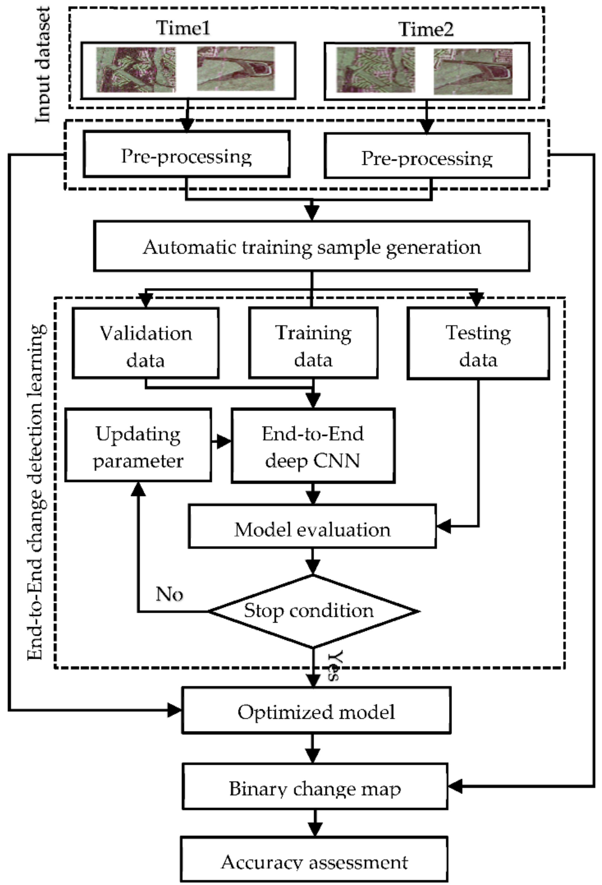
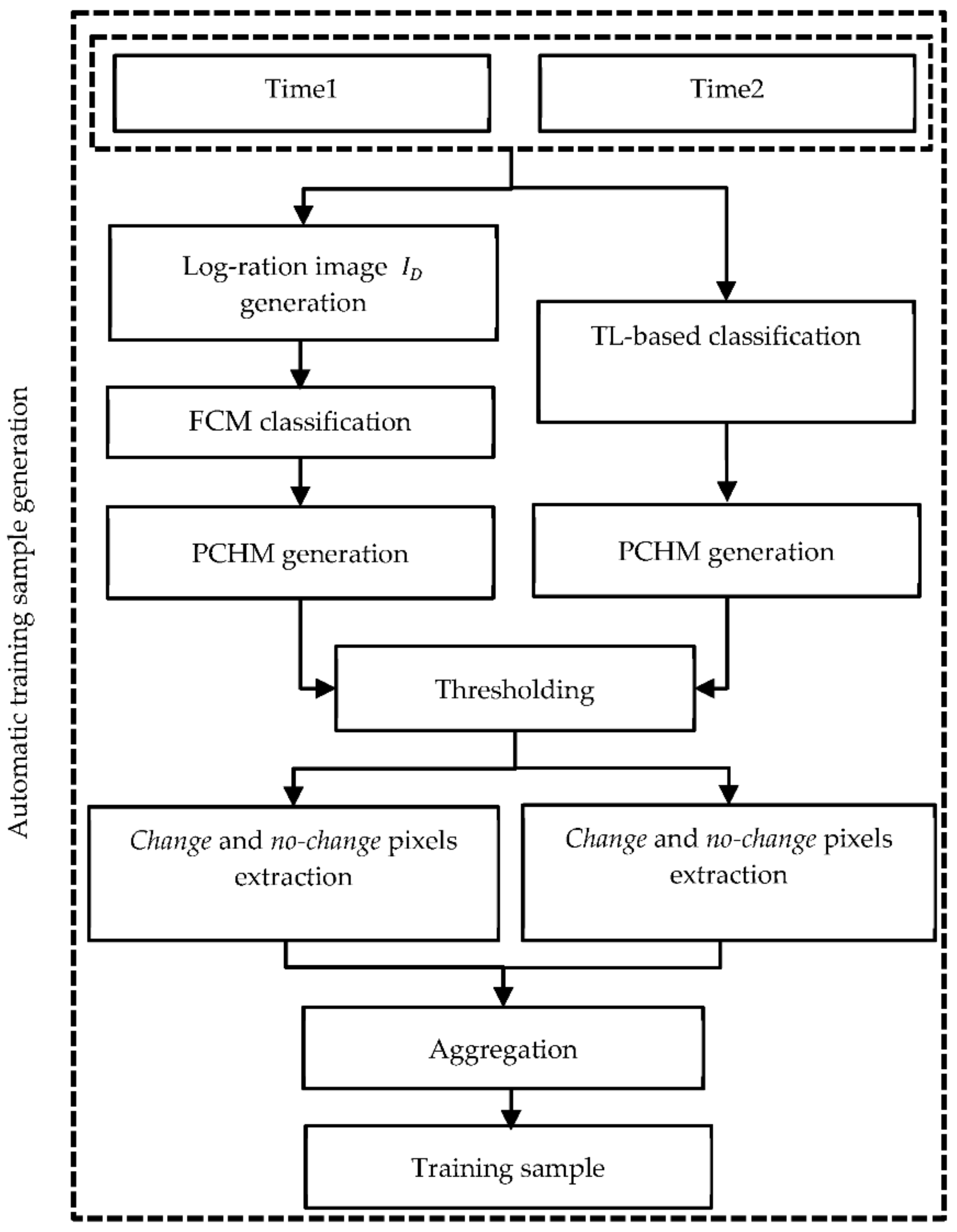
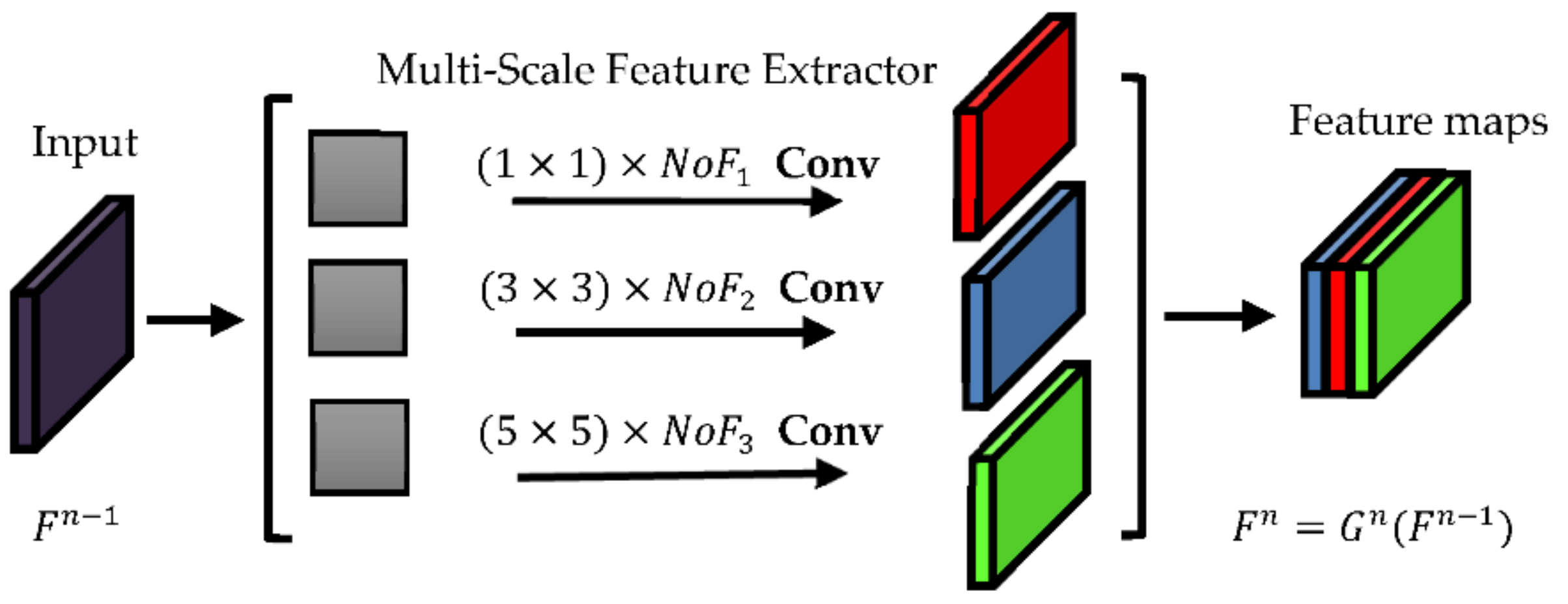
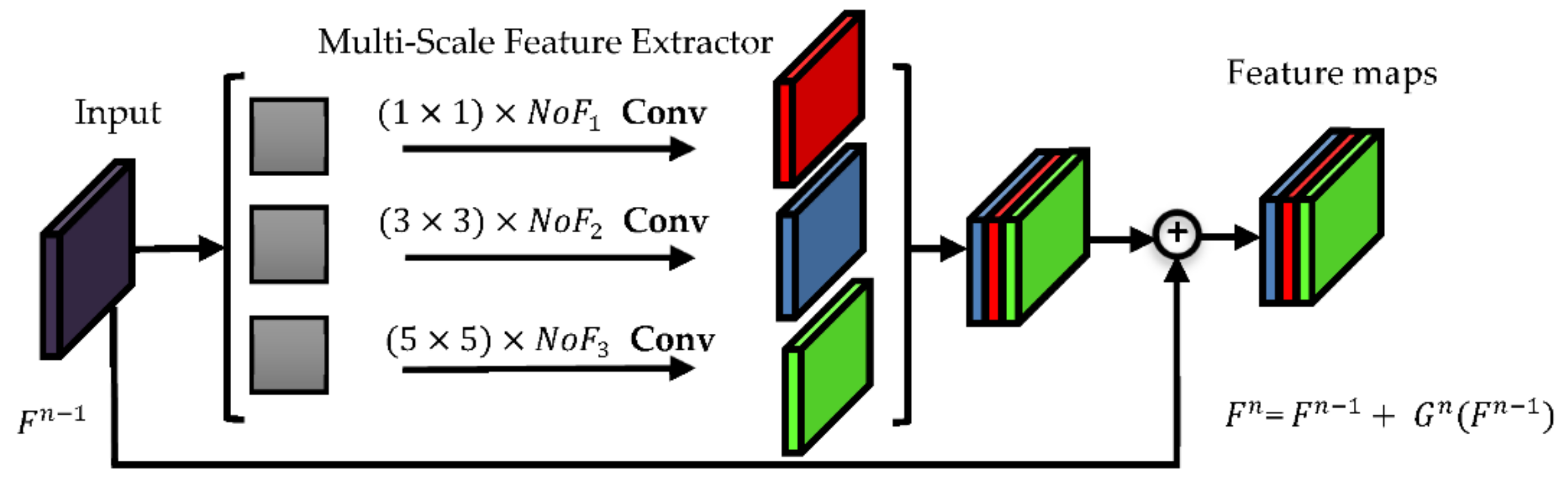
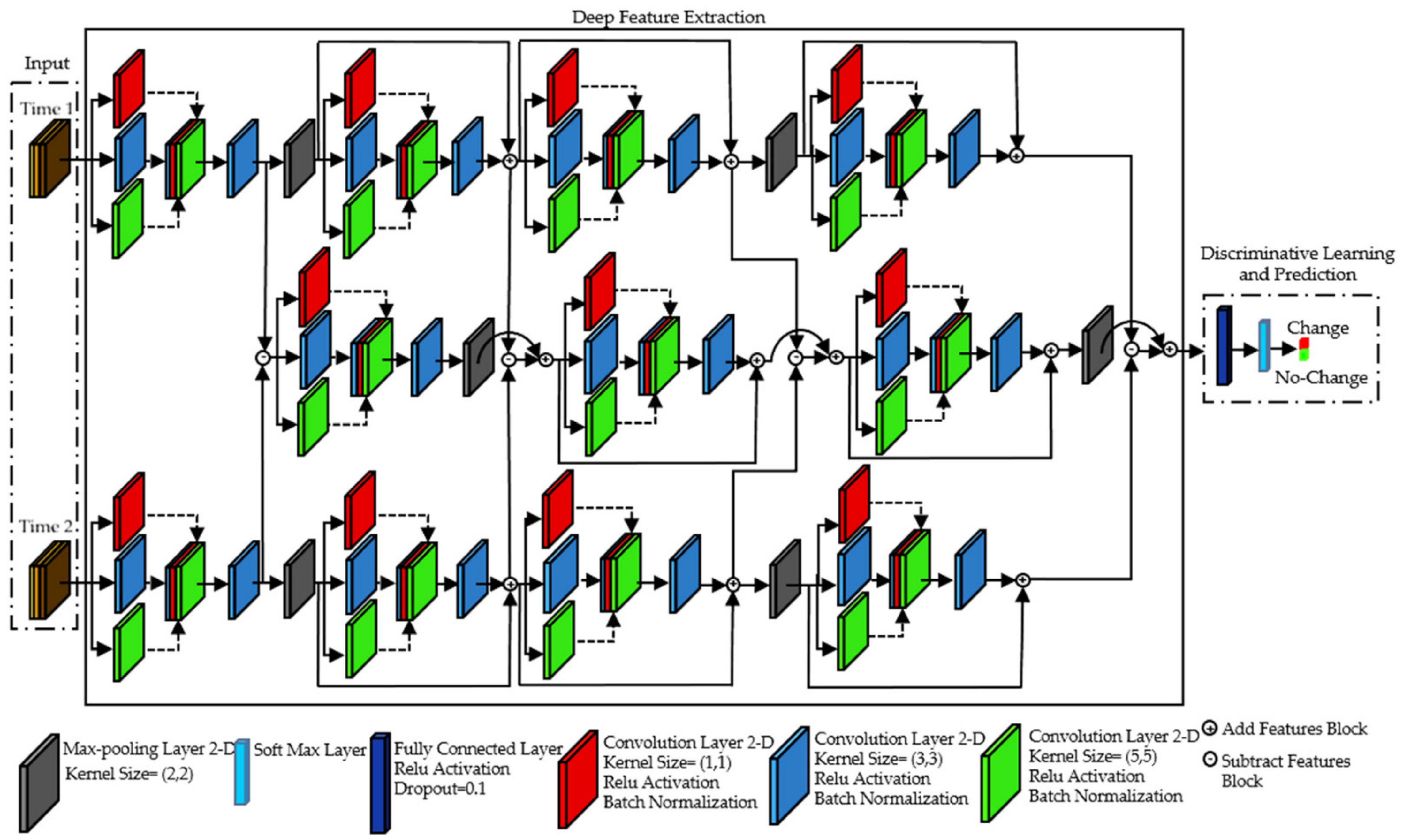
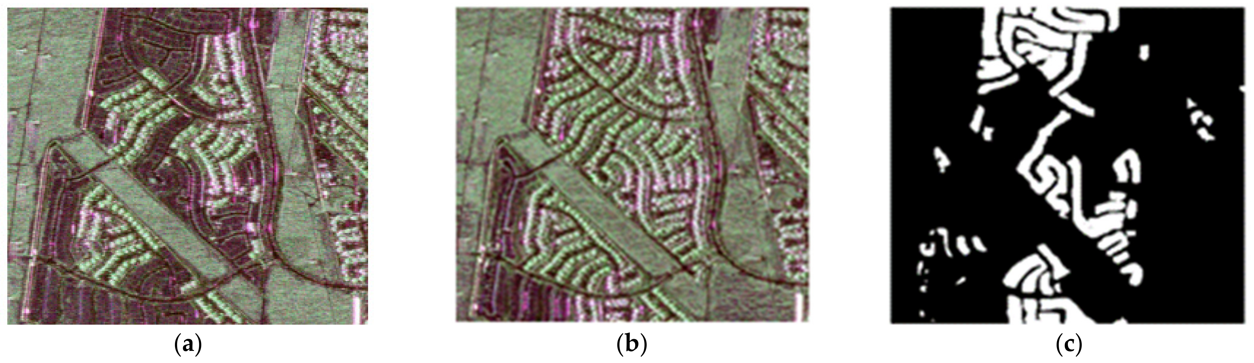
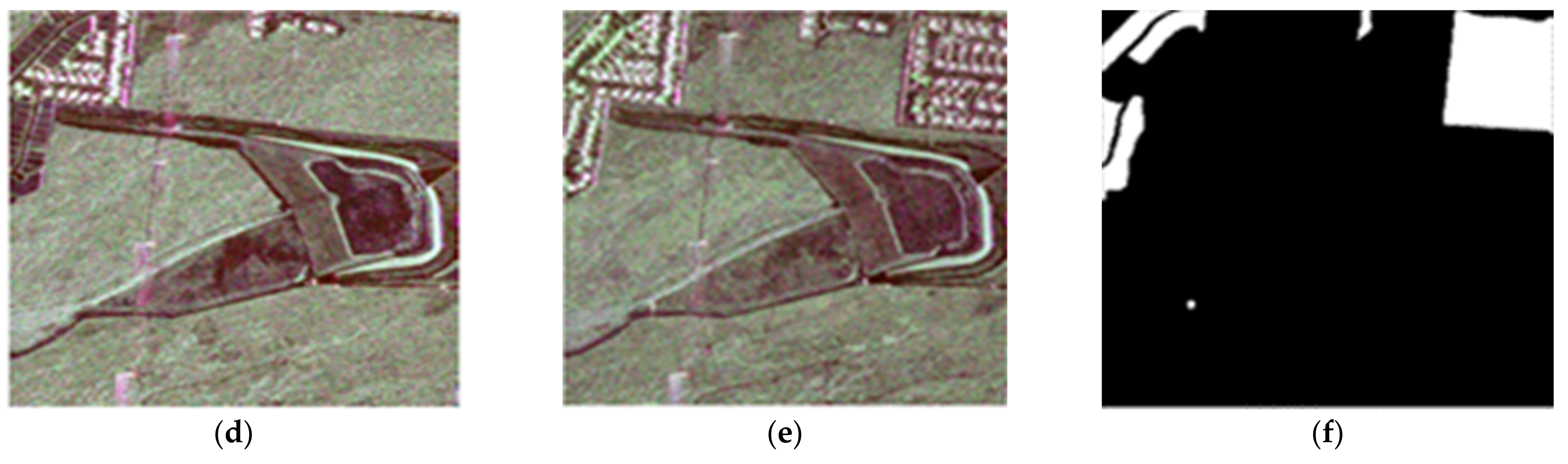
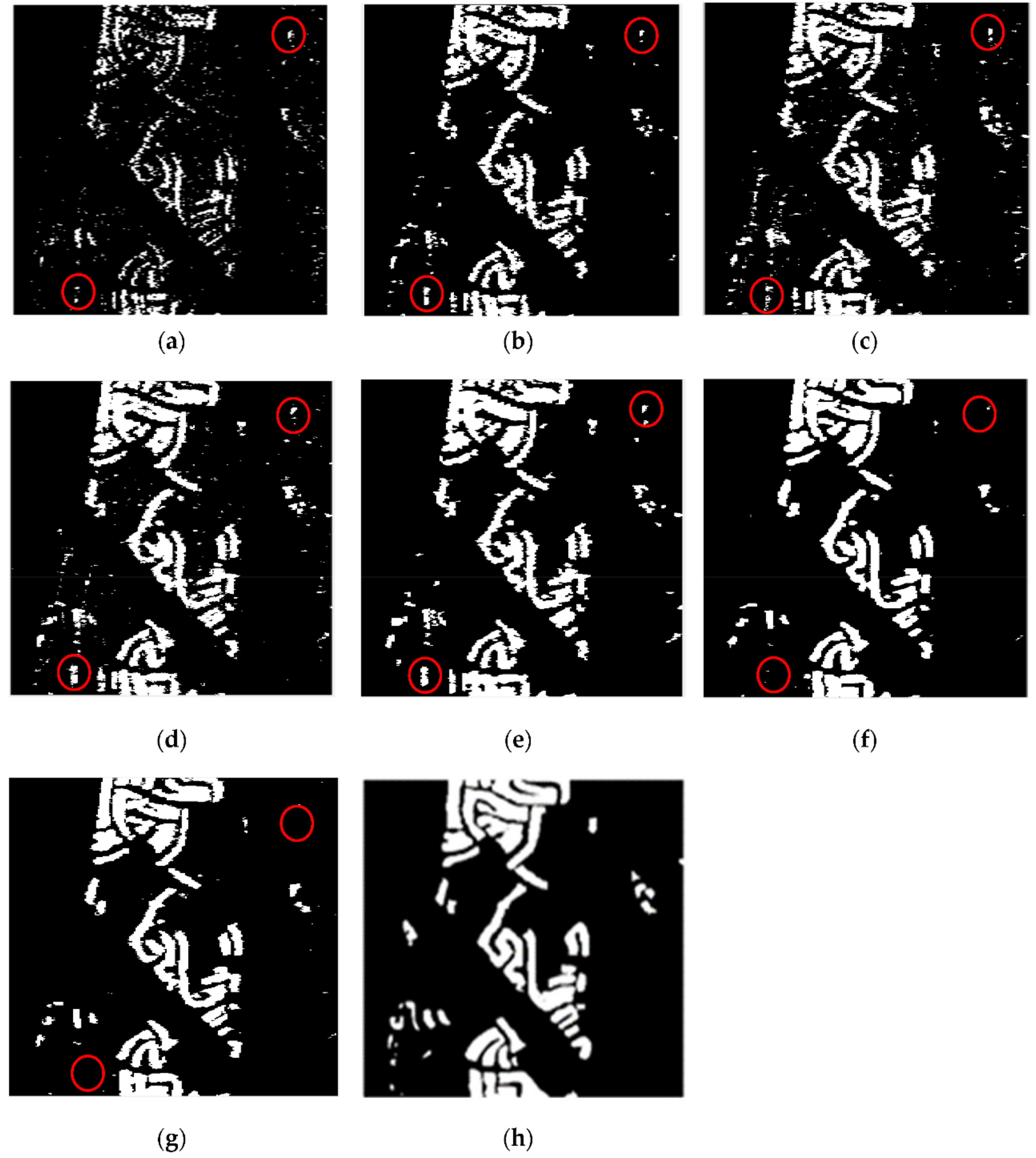
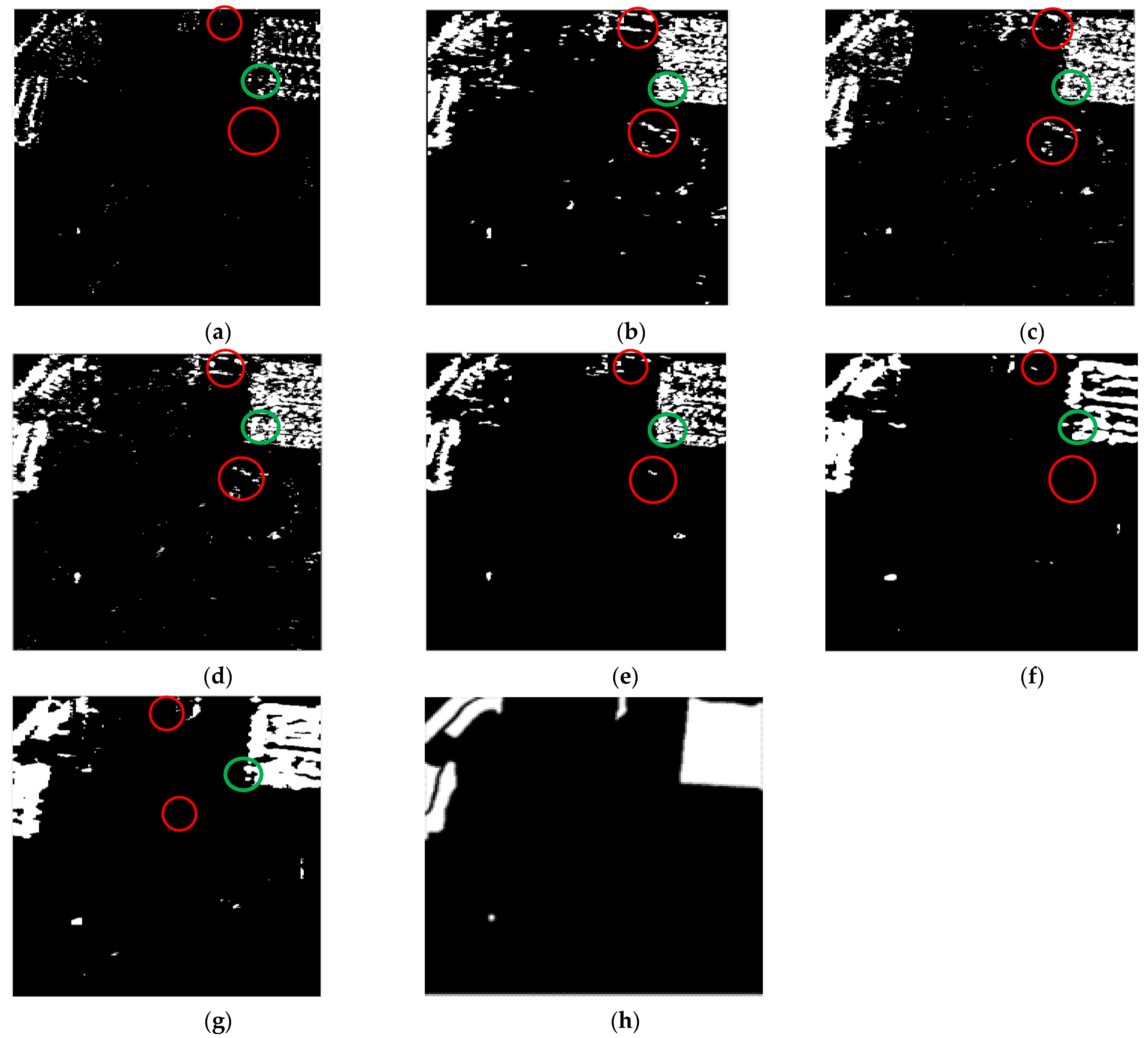
Table 1.
Formulas for accuracy assessment criteria.
| Accuracy Index | Formula |
|---|---|
| FNR | |
| TPR | |
| FPR | |
| OA | |
| Precision | |
| F1-Score | |
| OER | |
| PRE | |
| KC |
Table 2.
TCD-Net configurations of each channel and block.
| Channel 1 | Channel 2 | Channel 3 | |
|---|---|---|---|
| Inputs (shape) | |||
| Block 1 | Multi-Scale Shallow Block: ) 1 )) Channel Concat. 3 × 3 Conv4 + BN + RELU(256) | Multi-Scale Shallow Block: ) ) ) Channel Concat. 3 × 3 Conv4 + BN + RELU (256) | Multi-Scale Shallow Block: ) ) ) Channel Concat. 3 × 3 Conv4 + BN + RELU(256) |
| 2 × 2 Max-Pooling | 2 × 2 Max-Pooling | 2 × 2 Max-Pooling | |
| Output | 256 | 256 | 256 |
| Block 2 | Multi-Scale Residual Block: ) ) ) Channel Concat. 3 × 3 Conv4 + BN + RELU(256) | Multi-Scale Residual Block: ) ) ) Channel Concat. 3 × 3 Conv4 + BN + RELU(256) | Multi-Scale Residual Block: ) ) ) Channel Concat. 3 × 3 Conv4 + BN + RELU(256) |
| Output | |||
| Block 3 | Multi-Scale Residual Block: ) ) ) Channel Concat. 3 × 3 Conv4 + BN + RELU(256) | Multi-Scale Residual Block: ) ) ) Channel Concat. 3 × 3 Conv4 + BN + RELU(256) | Multi-Scale Residual Block: ) ) ) Channel Concat. 3 × 3 Conv4 + BN + RELU(256) |
| 2 × 2 Max-Pooling | 2 × 2 Max-Pooling | 2 × 2 Max-Pooling | |
| Output | 256 | 256 | 256 |
| Block 4 | Multi-Scale Residual Block:))) Channel Concat. 3 × 3 Conv4 + BN + RELU(256) | Multi-Scale Residual Block:) )) Channel Concat. 3 × 3 Conv4 + BN + RELU(256) | |
| Output | |||
| Flatten | |||
| Classifier | RELU Fully Connected (350) | ||
| Softmax Fully Connected (2) |
is the number of filters for convolutional layer of multi-scale block in channel of block.
Table 3.
The total number of filters in each multi-scale block.
| Block | Channel | ||
|---|---|---|---|
| 1 | 2 | 3 | |
| 1 | |||
| 2 | |||
| 3 | |||
| 4 | |||
Table 4.
The accuracy of the CD framework proposed in [2] for dataset#1 and dataset#2.
Table 4.
The accuracy of the CD framework proposed in [2] for dataset#1 and dataset#2.
| Method | Result | ||||||||||||
|---|---|---|---|---|---|---|---|---|---|---|---|---|---|
| TN | TP | FP | FN | TPR (%) | FPR (%) | FNR (%) | Precision | OA(%) | F1-Score | DR(%) | KC | OER (%) | |
| [2] dataset#1 | 187,570 | 27,606 | 11,581 | 9043 | 75.33 | 5.82 | 24.67 | 70.45 | 91.25 | 72.86 | 74.02 | 0.68 | 8.76 |
| [2] dataset#2 | 202,423 | 10,710 | 4188 | 12,479 | 46.19 | 2.03 | 53.81 | 71.89 | 92.75 | 56.24 | 29.22 | 0.52 | 7.25 |
Table 5.
The number of change and no-change pixels extracted from the parallel pseudo-label generation framework and the number of training, testing and validation pixels used in the training process of TCD-Net.
Table 5.
The number of change and no-change pixels extracted from the parallel pseudo-label generation framework and the number of training, testing and validation pixels used in the training process of TCD-Net.
| Dataset | Value | ||||||
|---|---|---|---|---|---|---|---|
| Class | Total Number of Pixels | Number of Samples | Percentage (%) | Training | Validation | Testing | |
| dataset#1 | change no-change | 36,649 199,151 | 12,717 165,308 | 34.70 83.01 | 1191 6472 | 357 1493 | 366 1991 |
| dataset#2 | change no-change | 23,189 206,611 | 11,156 81,650 | 48.11 39.52 | 753 6714 | 173 1549 | 231 2066 |
Table 6.
The accuracy of different change detection methods for dataset#1.
| Method | Result | ||||||||||||
|---|---|---|---|---|---|---|---|---|---|---|---|---|---|
| TN | TP | FP | FN | TPR (%) | FPR (%) | FNR (%) | Precision | OA (%) | F1-Score | DR (%) | KC | OER (%) | |
| PCA_kmeans | 196,839 | 12,223 | 2312 | 24,426 | 33.35 | 1.16 | 66.65 | 84.09 | 88.66 | 47.76 | 33.35 | 0.43 | 11.34 |
| NR_ELM | 195,411 | 22,066 | 3740 | 14,583 | 60.21 | 1.88 | 39.79 | 85.51 | 92.26 | 70.66 | 60.21 | 0.66 | 7.74 |
| Gabor_PCANet | 192,837 | 23,449 | 6314 | 13,200 | 63.98 | 3.17 | 36.02 | 78.79 | 91.72 | 70.62 | 63.98 | 0.65 | 8.28 |
| DP_PCANet | 192,994 | 25,298 | 6157 | 11,351 | 69.03 | 3.09 | 30.97 | 80.43 | 92.58 | 74.29 | 69.03 | 0.69 | 7.42 |
| CWNN | 193,141 | 25,603 | 6010 | 11,046 | 69.86 | 3.02 | 30.14 | 80.99 | 92.77 | 75.01 | 69.86 | 0.70 | 7.23 |
| Dual-channel Net | 195,818 | 26,424 | 3333 | 10,225 | 72.10 | 1.67 | 27.90 | 88.80 | 94.25 | 79.58 | 72.10 | 0.76 | 5.75 |
| TCD-Net | 196,646 | 27,390 | 2505 | 9259 | 74.74 | 1.26 | 25.26 | 91.62 | 95.01 | 82.32 | 74.74 | 0.80 | 4.99 |
Table 7.
The accuracy of different change detection methods for dataset#2.
| Method | Result | ||||||||||||
|---|---|---|---|---|---|---|---|---|---|---|---|---|---|
| TN | TP | FP | FN | TPR (%) | FPR (%) | FNR (%) | Precision | OA (%) | F1-Score | DR (%) | KC | OER (%) | |
| PCA_kmeans | 205,826 | 5653 | 785 | 17,536 | 24.38 | 0.38 | 75.62 | 87.81 | 92.03 | 57.16 | 24.38 | 0.35 | 7.97 |
| NR_ELM | 200,774 | 15,525 | 837 | 7664 | 66.95 | 2.83 | 33.05 | 72.68 | 94.12 | 83.85 | 66.95 | 0.66 | 3.70 |
| Gabor_PCANet | 202,050 | 14,884 | 4511 | 8355 | 64.05 | 2.18 | 35.95 | 76.74 | 94.40 | 78.47 | 64.19 | 0.67 | 5.60 |
| DP_PCANet | 202,383 | 15,019 | 4228 | 8170 | 64.77 | 2.05 | 35.23 | 78.03 | 94.60 | 80.32 | 64.77 | 0.68 | 5.40 |
| CWNN | 204,199 | 13,060 | 2412 | 10,129 | 56.32 | 1.17 | 43.68 | 84.41 | 94.54 | 80.33 | 56.32 | 0.65 | 5.46 |
| Dual-channel Net | 203,880 | 15,460 | 2731 | 7729 | 66.67 | 1.32 | 33.33 | 84.99 | 95.45 | 74.72 | 66.67 | 0.72 | 4.55 |
| TCD-Net | 203,284 | 18,949 | 3327 | 4240 | 81.72 | 1.61 | 18.28 | 85.06 | 96.71 | 87.86 | 81.72 | 0.82 | 3.29 |
Table 8.
Comparison of TCD-Net results with other methods developed on UAVSAR images.
| Dataset | Indices | Result | |||
|---|---|---|---|---|---|
| Ratha, De, Celik and Bhattacharya [68] | Bouhlel, Akbari and Méric [3] | Nascimento, Frery and Cintra [69] | TCD-Net | ||
| dataset#1 | KC FPR (%) DR (%) | 0.73 6.9 N/A | N/A 10.58 63.38 | 0.62 4.14 42.98 | 0.80 1.26 74.74 |
| dataset#2 | KC FPR (%) DR (%) | 0.75 3.9 N/A | N/A 8.39 51.49 | 0.56 2.17 62.52 | 0.82 1.61 81.72 |
Publisher’s Note: MDPI stays neutral with regard to jurisdictional claims in published maps and institutional affiliations. |
© 2022 by the authors. Licensee MDPI, Basel, Switzerland. This article is an open access article distributed under the terms and conditions of the Creative Commons Attribution (CC BY) license (https://creativecommons.org/licenses/by/4.0/).
Share and Cite
MDPI and ACS Style
Habibollahi, R.; Seydi, S.T.; Hasanlou, M.; Mahdianpari, M. TCD-Net: A Novel Deep Learning Framework for Fully Polarimetric Change Detection Using Transfer Learning. Remote Sens. 2022, 14, 438. https://doi.org/10.3390/rs14030438
AMA Style
Habibollahi R, Seydi ST, Hasanlou M, Mahdianpari M. TCD-Net: A Novel Deep Learning Framework for Fully Polarimetric Change Detection Using Transfer Learning. Remote Sensing. 2022; 14(3):438. https://doi.org/10.3390/rs14030438
Chicago/Turabian StyleHabibollahi, Rezvan, Seyd Teymoor Seydi, Mahdi Hasanlou, and Masoud Mahdianpari. 2022. "TCD-Net: A Novel Deep Learning Framework for Fully Polarimetric Change Detection Using Transfer Learning" Remote Sensing 14, no. 3: 438. https://doi.org/10.3390/rs14030438
Note that from the first issue of 2016, this journal uses article numbers instead of page numbers. See further details here.