Evaluation of SMOS L4 Sea Surface Salinity Product in the Western Iberian Coast

Abstract

Salinity is one of the oldest parameters being measured in oceanography and one of the most important to study in the context of climate change. However, its quantification by satellite remote sensing has been a relatively recent achievement. Currently, after over ten years of data gathering, there are still many challenges in quantifying salinity from space, especially when it is intended for coastal environments study. That is mainly due to the spatial resolution of the available products. Recently, a new higher resolution (5 km) L4 SMOS sea surface salinity (SSS) product was developed by the Barcelona Expert Center (BEC). In this study, the quality of this product was tested along the Western Iberian Coast through its comparison with in situ observations and modelled salinity estimates (CMEMS IBI Ocean Reanalysis system). Moreover, several parameters such as the temperature and depth of in situ measurements were tested to identify the variables or processes that induced higher errors in the product or influenced its performance. Lastly, a seasonal and interannual analysis was conducted considering data between 2011 to 2019 to test the product as a potential tool for long-term studies. The results obtained in the present analysis showed a high potential of using the L4 BEC SSS SMOS product in extended temporal and spatial analyses along the Portuguese coast. A good correlation between the satellite and the in situ datasets was observed, and the satellite dataset showed lower errors in retrieving coastal salinities than the oceanic model. Overall, the distance to the coast and the closest rivers were the factors that most influenced the quality of the product. The present analysis showed that great progress has been made in deriving coastal salinity over the years and that the SMOS SSS product is a valuable contribution to worldwide climatological studies. In addition, these results reinforce the need to continue developing satellite remote sensing products as a global and cost-effective methodology for long-term studies.

1. Introduction

Salinity plays an extremely important role in the overall dynamics of our oceans. Together with temperature, salinity directly affects the water density and, therefore, the circulation in the ocean. Thus, it is one of the key variables to monitor and model ocean circulation [1]. In addition, surface salinity is strongly linked to the water cycle, mainly through evaporation and precipitation processes [2]. It is a vital element for balancing all ecosystems and their organisms, and it varies in place and time, showing seasonal and interannual variability [3,4]. These variations result from evaporation and dilution by freshwater (rain and river runoff), processes that occur at the surface of the ocean [3]. These changes are critical drivers of oceanic circulation [5]. Given the importance of salinity as an essential climate variable [6], both time and resources need to be invested in studying its variability. Recognizing how salinity varies worldwide is essential to understanding climate change [7].

The quantification of sea surface salinity (SSS) through satellite remote sensing has emerged as a cost-effective complement to in situ cruises, which alone are insufficient to gather synoptic continuous and regular time series [1]. However, achieving this goal was a time-consuming process. In 1995, quantifying salinity from space was considered “the next challenge” in satellite remote sensing [8]. Only fourteen years later, it was possible to measure sea surface salinity from space, using L-band microwave measurements with the launch of ESA’s Soil Moisture and Ocean Salinity (SMOS) mission in November 2009 [9] with a mean spatial and temporal resolution of 43 km and 3–5 day (revisit time), respectively [10]. Currently, it is also possible to obtain salinity data from the Aquarius and SMAP missions (NASA) [11]. Aquarius (2011–2015) had a 100–150 km spatial resolution and a 7-day exact repeat. SMAP (2015–present) has a spatial resolution of 40 km and a repeat cycle of 2–3 days [10,12]. Nevertheless, retrieving salinity data in near coastal regions remains a challenge due to the dynamic nature of coastal processes [13,14]. The high variability in reduced spatial and temporal scales, enhanced by the influence of river discharges and land runoff, makes it difficult to monitor these environments using satellite products. These constraints are noted by Olmedo et al. [15], who state that the available SMOS SSS does not capture the dynamics of most coastal pixels of the Portuguese coast. Bao et al. [12] also found large discrepancies between SMOS, Aquarius, and SMAP and in situ observations in worldwide coastal regions (higher root-mean-square error (RMSE) than for the open ocean). Sources of error in the quantification of SSS can result from disturbances in the algorithm’s performance due to solar and sky emissions, the Faraday rotation in the ionosphere, the impact of the atmosphere and the effect of sea surface roughness on L-band emissivity [11]. Particularly, SSS coastal measurements are affected by land contamination and high levels of radio frequency interference [11,16,17]. These two factors are the main limitation in obtaining high-quality coastal salinity retrievals [18]. To surpass these constraints, reanalysis products are often used to quantify sea surface salinity (e.g., [19]). Copernicus Marine Environment Monitoring Service (CMEMS) provides multiyear global and regional reanalysis products with physical and biogeochemical parameters, including salinity [20]. One regional product is available for the Iberian Region (IBI—Iberia-Biscay-Ireland seas) [21]. However, despite its appealing temporal coverage and the 8.3 km/1 day spatial and temporal resolution, the enhancement of land forcing in this type of model, including river discharges, is identified as a priority objective to improve the quality of coastal salinity quantification [20].

Compensating for all these limitations, a new and higher resolution SMOS global L4 product was developed by the Barcelona Expert Center as a result of merging the SMOS salinity data with Operational Sea Surface Temperature and Ice Analysis (OSTIA) data [22]. Thus, the main goal of the present study is to evaluate the performance of this product in the coastal region of the Western Iberian Coast (WIC) and assess the salinity spatial, seasonal, and interannual variability, testing the product as a potential tool for cost-effective long-term analysis. The product’s performance was tested through the comparison with concomitant in situ observations and data from the CMEMS IBI reanalysis product [21]. The suitability of the product for seasonal and interannual analyses was assessed aiming to consolidate the product quality and increase the knowledge of coastal salinity variability, as this was the first study conducted with this new product in this coastal region and one of the few ever published works focused on the study of the salinity patterns along the Portuguese coast. The research was guided by the following questions: (i) Can this product be used as a reliable complement to the in situ campaigns? (ii) Does this product retrieve higher quality coastal salinities than the model-derived salinity products currently available for the WIC? (iii) Which factors mainly affected the errors in the quantification of SSS? (iv) What are the seasonal and interannual patterns of SSS in the WIC?

2. Data and Methodology

2.1. Study Site

The Iberian Peninsula is located in the southwest of Europe, with Portugal occupying its western region (Figure 1). The Portuguese coast is washed by the Atlantic Ocean and is marked by several estuaries and capes that affect the circulation patterns and the variability of the physical and biological properties of the region [23]. There is some significant freshwater input from the main rivers: Douro, Tagus, Mondego, Sado, and Mira estuaries, as well as Ria de Aveiro and Ria Formosa.

The west coast of the Iberian Peninsula is part of the Eastern North Atlantic Boundary [23]. During the winter season (September/October–April/May), the prevailing winds are mainly westerly and southerly, generating the Iberian poleward current (IPC) [24,25], resulting in a predominantly northward turning surface circulation in the WIC [26]. This current system transports warmer and saltier waters and is characterized by flow instabilities, eddy interactions, and shedding and separation from the slope [24,25]. During spring and summer (April/May–September/October), the Western Iberian Coast is characterized by northerly winds that force upwelling events, with colder and nutrient-rich subsurface waters [24,25,27]. This process starts with the formation of a narrow band of cold water along the coast that initiates destabilization, resulting in the formation of small-scale disturbances along the thermal front. After approximately one month of prevailing equatorward winds, filaments start to develop with associated cross-shore currents. The presence of multiple filaments of cold water that extend over 200 km offshore is recurrent [24].

On the other hand, the south coast of Portugal (included in the Gulf of Cadiz) shows different circulation patterns, and Cape Santa Maria divides the continental shelf into two parts that present different circulation regimes. During spring and summer, the surface circulation over the continental shelf presents two cells of cyclonic circulation (separated by Cape Santa Maria), coupled to the open sea surface circulation [28]. In the outer Gulf of Cadiz, a generalized anticyclonic circulation in the basin is observed, driven by the upwelling jet formed during that time of the year on the west coast that spreads eastwards along the coast [29]. During winter, the flow that tends to move southeast often flows towards the northwest due to the change of the prevailing winds, reversing the direction of the coastal counter current in the east cell of the continental shelf [28]. For additional information regarding the circulation regime and the seasonal wind field of the WIC, see Peliz et al. [30], Criado–Aldeanueva et al. [29] and Sánchez et al. [31].

The river runoff produces lenses of low salinity water along the coastal ocean called buoyant plumes. In the Iberian Peninsula, most of the river flow occurs in its northern segment, where a recurrent plume is observed (salinities < 35.8) [24]. In the last two decades, there has been an increase in the frequency and intensity of drought situations in Portugal. In addition, a reduction in the amount of precipitation has been detected [32], suggesting a consequent decrease in the rivers flow. According to Koppen’s classification, mainland Portugal is characterized as having a temperate climate of rainy winters and dry summers (hot or less hot, according to the region of the country) [33].

2.2. In Situ Salinity Data

Salinity profiles were determined using a CTD (for conductivity, temperature, and depth), during three oceanographic cruises conducted in October 2018 (Autumn 2018), April/May 2019 (Spring 2019), and October 2019 (Autumn 2019). In each cruise, sampling was conducted along five different regions, named A to E. These regions are distributed along the Portuguese coast (Figure 1), with A being the northernmost region and E being the southernmost one. The Autumn cruises lasted 22 days, while the Spring 2019 cruise ran for 25 days. The region’s sampling order followed the sequence: Autumn 2018—E, D, C, A and B; Spring 2019—E, D, B, A and C; Autumn 2019—E, B, A, C and D.

For the present analysis, only the shallowest valid value of each salinity profile was used (values gathered between 4 and 8 m depth). All CTD data were submitted to validation and processing procedures using a program developed by the Division of Oceanography at Instituto Hidrográfico (IH). After processing the data, automatic quality control was carried out, adding a flag 1, 2, 4, and 9 to each record. The quality flags were considered taking into account the number of records used for subsequent compaction. It was considered that the number of records for each compression interval was approximately N = pcom/tinc, depending on the time increment (tinc) and on the compression interval (pcom) at a descent rate in the order of 1 m/s. The flags evaluated the data as follows: 9—Missing value (indicated that all records used in the compaction were invalid); 4—Bad (indicated that the number of records used was <1/3 of N); 2—Suspicious (indicated that the number of registers used was 1/3 < N < 1/2); 1—Good (indicated that the number of registers used was ≥1/2). Only data flagged 1 were considered in our analysis.

2.3. Satellite-Derived Salinity Data

The satellite-derived sea surface salinity data used was produced and distributed by the Barcelona Expert Centre (BEC) team through its data visualization and distribution service (http://bec.icm.csic.es/bec-ftp-service/, accessed on 2 July 2021). Specifically, data from version 2 of a level 4 (L4) product that resulted from merging the SMOS salinity data (0.25° × 0.25°) with OSTIA sea surface temperature (0.05° × 0.05°) was used [22,34]. The product has a spatial resolution of 5 km, a temporal resolution of 1 day and full temporal coverage of 9 years, with data available between 2011 and 2019. Hereafter, the product will be referred to as SMOS SSS.

The Level 4 product was generated using the multifractal fusion method introduced in Umbert et al. [35]. The method starts with the assumption that two different ocean scalars at the same place and time should have the same Singularity Exponents [36]. Roughly speaking, since the singularity exponents represent the degree of regularity of a turbulent flow, this assumption says that the turbulence of the ocean is manifested in the same way in the different physical properties of the sea. This assumption was confirmed in different studies [37,38]. Initially, multifractal fusion was introduced in the SMOS SSS maps for reducing the noise of the Level 3 SMOS SSS products [35,36]. However, Olmedo et al. [39] showed that after applying multifractal fusion to the Level 3 SMOS SSS, the resulting SMOS SSS L4 maps inherited the effective spatial resolution and the temporal resolution of the ocean scalar used as a template, SST in this case.

Olmedo et al. [22] compared and assessed the performance of the BEC SMOS SSS L4 product with those of other satellite SSS L3 products. The results showed that at a global scale, in terms of biases (i.e., mean difference with respect to in situ salinity measurements), this product presented similar performances to the rest of satellite salinity products. However, in terms of the standard deviation of the error, the product performed better than the analyzed satellite salinity products. Two metrics were used for the latter analysis: (i) the computation of the standard deviation of the difference between satellite and in situ salinity measurements, and (ii) correlated triple collocation analysis [40]. The authors also performed spectral and singularity [41] analysis and concluded that, while the effective spatial resolution of the analyzed L3 satellite salinity products was around 40 km, that of the L4 was very similar to the SST used in the multifractal fusion scheme, which was around 20 km.

While the quality assessment presented in Olmedo et al. [22] focused on the performance in the global ocean, here, this product is assessed in relation to its performance in a coastal region. Thus, in particular, this study analyzes whether the product still presents residual Land-Sea-Contamination and, despite its limitations, if it yields better performance than the available models for the region (i.e., IBI, as described below).

2.4. Modelled Salinity Data

Data from the Iberian Biscay Irish (IBI) Ocean Reanalysis system were also considered to compare with satellite and in situ salinity data (Product identifier-IBI_MULTIYEAR_PHY_005_002). This numerical model provides daily mean surface salinity data with a spatial resolution of 8.3 km. It has available data starting with 1993, and it was produced and distributed by E.U. Copernicus Marine Service (https://resources.marine.copernicus.eu/products, accessed on 10 August 2021) [21].

2.5. Matchups Analysis

The search for matchups (spatial and temporal coincident observations) was conducted by comparing the in situ observations with the satellite/modelled data obtained for the same day and the same location (single-pixel analysis). In the cases where several same-day in situ measurements coincided in the same pixel of the satellite/model grid, i.e., several in situ values were matched with the same satellite/model value, the mean of the in situ values was considered (spatial average of the in situ observations). This processing step was practically negligible with the satellite (12 cases out of 711 cases) but evident with the model data due to its worse spatial resolution (126 cases out of 711 data matchups). Neither the satellite nor the model allowed estuarine analysis along the Portuguese coast due to their spatial coverage and resolution.

During this analysis, 77% of good matchups were obtained, both for the satellite and the model. The invalid satellite matchups resulted from the lack of resolution of the satellite data for near coast measurements. As for the model, the invalid matchups resulted from the lower spatial resolution of the product (in comparison with the satellite), causing several in situ observations to correspond to the same measurement (same pixel) of the modelled data, even though the model was able to acquire salinities much closer to the coast than the satellite.

2.6. Statistical Analysis

The relation between the in situ salinity observations and the satellite-derived and the modelled salinity data was evaluated with statistical analysis, considering the Root Mean Square Error (RMSE), Bias Error (BIAS), Absolute Percentage Difference (APD) and Relative Percentage Difference (RPD), following:

$$RMSE=\sqrt{\frac{{\displaystyle {\displaystyle \sum }_{i=1}^N}{\left(S_{derive{d}_i}-S_{in sit{u}_i}\right)}^2}{N}}$$

(1)

$$BIAS=\frac{1}{N}{\displaystyle \sum }_{i=1}^N\left(S_{derive{d}_i}-S_{in sit{u}_i}\right)$$

(2)

$$APD\left(\%\right)=\frac{1}{N}{\displaystyle \sum }_{i=1}^N\frac{\left|S_{derive{d}_i}-S_{in sit{u}_i}\right|}{S_{in sit{u}_i}}\times 100$$

(3)

$$RPD\left(\%\right)=\frac{1}{N}{\displaystyle \sum }_{i=1}^N\frac{S_{derive{d}_i}-S_{in sit{u}_i}}{S_{in sit{u}_i}}\times 100$$

(4)

where S_derived expresses the satellite or the model-derived salinity data, S_{in situ} the in situ observations, N the total number of matchups considered and i the matchup index. RMSE and bias error were considered as uncertainty estimates: the RMSE was selected to determine the data spread (precision) and the bias error to estimate the data offset (accuracy) [42]. As a complement, RPD was used as an indicator of the systematic error, while APD was also considered as an accuracy parameter. The matchup analysis included the assessment of linear regression parameters, as the slope, the intercept, and the determination coefficient (R²).

2.7. Error-Related Factors

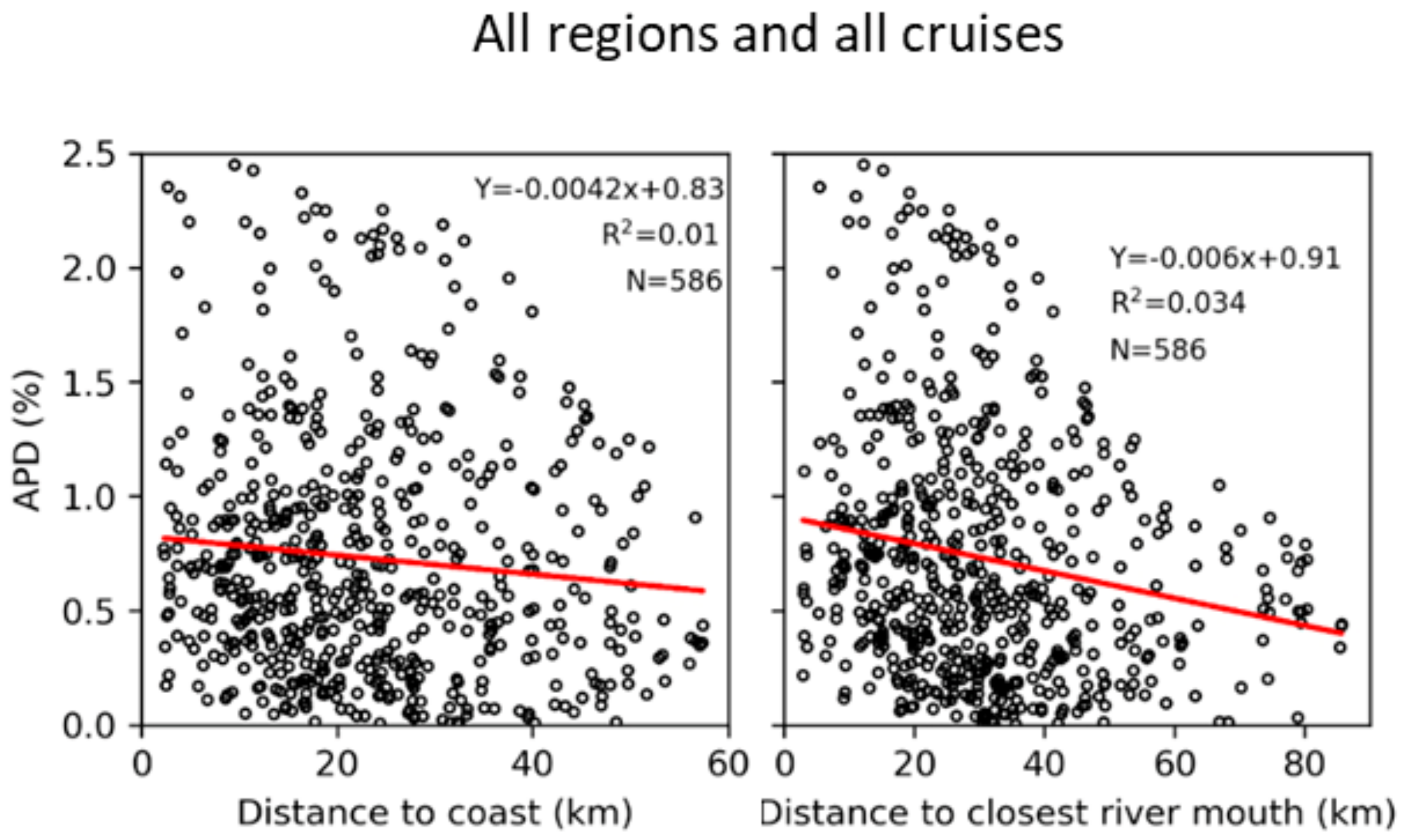
Aiming to understand which factors were affecting the quality of the satellite product, the APD of each matchup was compared with several parameters: (i) depth at which the in situ observations were made; (ii) distance to coast; (iii) distance to main rivers; (iv) temperature. Note that hypothetical higher differences between the satellite and the in situ measurements gathered at larger depths would not indicate the origin of the satellite error but rather that the water column could be stratified. In such a case, it would not be entirely appropriate to compare the two datasets. These issues need to be analyzed with care, given that the satellite product provides data for the first centimeters of the water column, while the in situ observations were conducted at up to 8 m depth. Analogously, higher differences between satellite and in situ measurements closer to main rivers could represent the residual land–sea contamination in the satellite measurements. These regions are typically characterized by fast salinity dynamics and are rich in small spatial structures. However, large differences near rivers could also be associated with differences in the spatial and temporal scales that are being compared, i.e., SMOS L4 SSS product provides an integrated measure of one day in an area of around 5 × 5 km and the in situ data represents punctual and instantaneous observations.

To account for the distance to the main rivers and secondary freshwater outflows, the following rivers were considered: Guadiana, Ribeira de Odiáxere, Ribeira da Quarteira, Ria Formosa, Gilão, Arade, Mira, Sado, Tagus, Mondego, Ria de Aveiro, Douro, Ave, Cávado, Lima, and Minho (see Figure S1 in the Supplementary Materials). Both the distance of the observations to the coast and the closest rivers was obtained considering the nearest neighbor method.

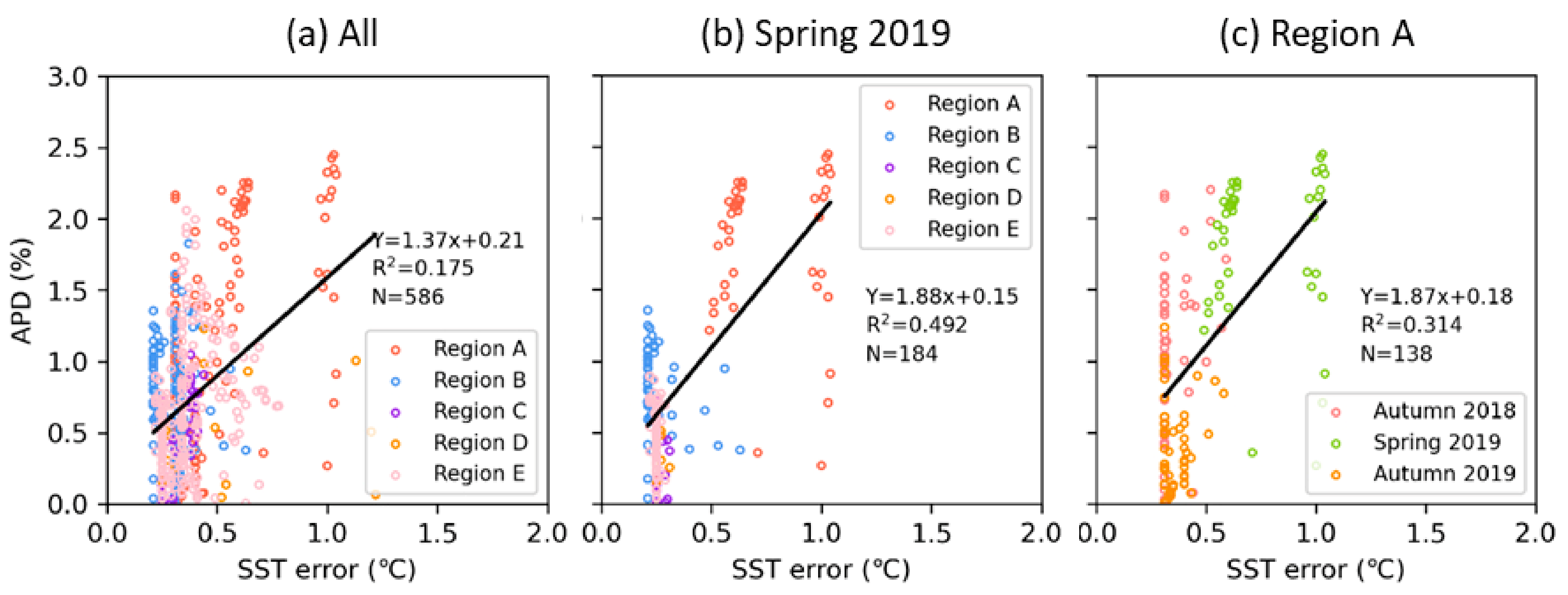
Temperature data were collected using a CTD, along with conductivity (from which salinity was determined). Version 2 of OSTIA product (https://resources.marine.copernicus.eu/products [43,44], accessed on 27 September 2021) was also considered in the present analysis to investigate whether the sea surface temperature data used in the creation of the product could influence the quality of SSS fields. The product allows for daily fields of sea surface temperature with 5 km spatial resolution (data available since 2007 for the Near Real-Time product). In the present analysis, it was considered the estimated error standard deviation of the analyzed SST.

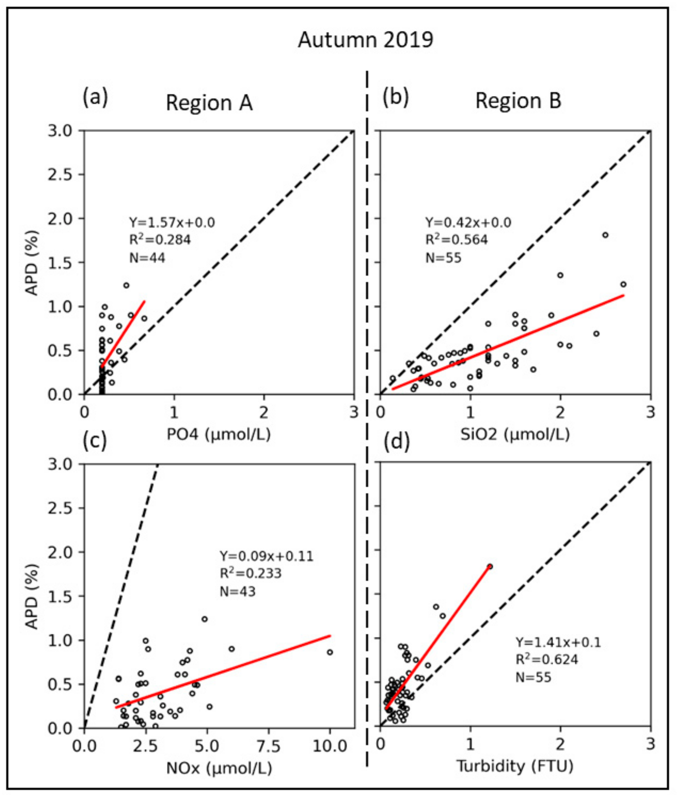
2.8. Salinity Links with Biochemical Variables

To test if oceanographic and environmental processes (e.g., upwelling, river discharges) were affecting the quality of the satellite data and to test the capability of the satellite in quantifying salinity under the influence of such seasonal processes, the following parameters were compared with the APD of each matchup: (a) turbidity; (b) nutrients (phosphate (PO₄), total oxidized nitrogen (NO_x) and silicate (SiO₂)); (c) chlorophyll a; (d) daily average river flow. These biochemical variables were collected during the cruises and used as indicators of processes that usually affect the variability of salinity along the Portuguese coast.

Turbidity data was collected using the SEAPOINT OEM Turbidity meter. This sensor detects light scattered by particles suspended in water, generating an output voltage proportional to turbidity or suspended solids. The quantification of the nutrients was made by UV/Vis spectrometry using specific colorimetric methods implemented in a Skalar SANplus Segmented Flow Auto-Analyzer. NO_x was quantified according to Strickland and Parsons [45] and SiO₂ and PO₄ according to Murphy and Riley [46]. Chlorophyll a was retrieved by absorption spectrometry following a modification of Lorenzen’s approach [47,48] using a ThermoFisher Scientific Evolution 201 UV-Visible Spectrophotometer.

Additionally, the daily average water flow (m³/s) for several major rivers along the WIC (Douro, Mondego, Tagus, and Guadiana) between 2011–2019 were extracted from the Portuguese National Water Resources Information System (SNIRH; available at: www.snirh.apambiente.pt, accessed on 25 October 2021) and compared to nearby concomitant SSS measurements (single-pixel analysis).

2.9. Seasonal and Interannual Analysis

To evaluate the product as a potential tool for cost-effective long-term analysis, aiming to increase knowledge about the variability of coastal salinity in the WIC, an analysis of the temporal variability of salinity was conducted using different time scales.

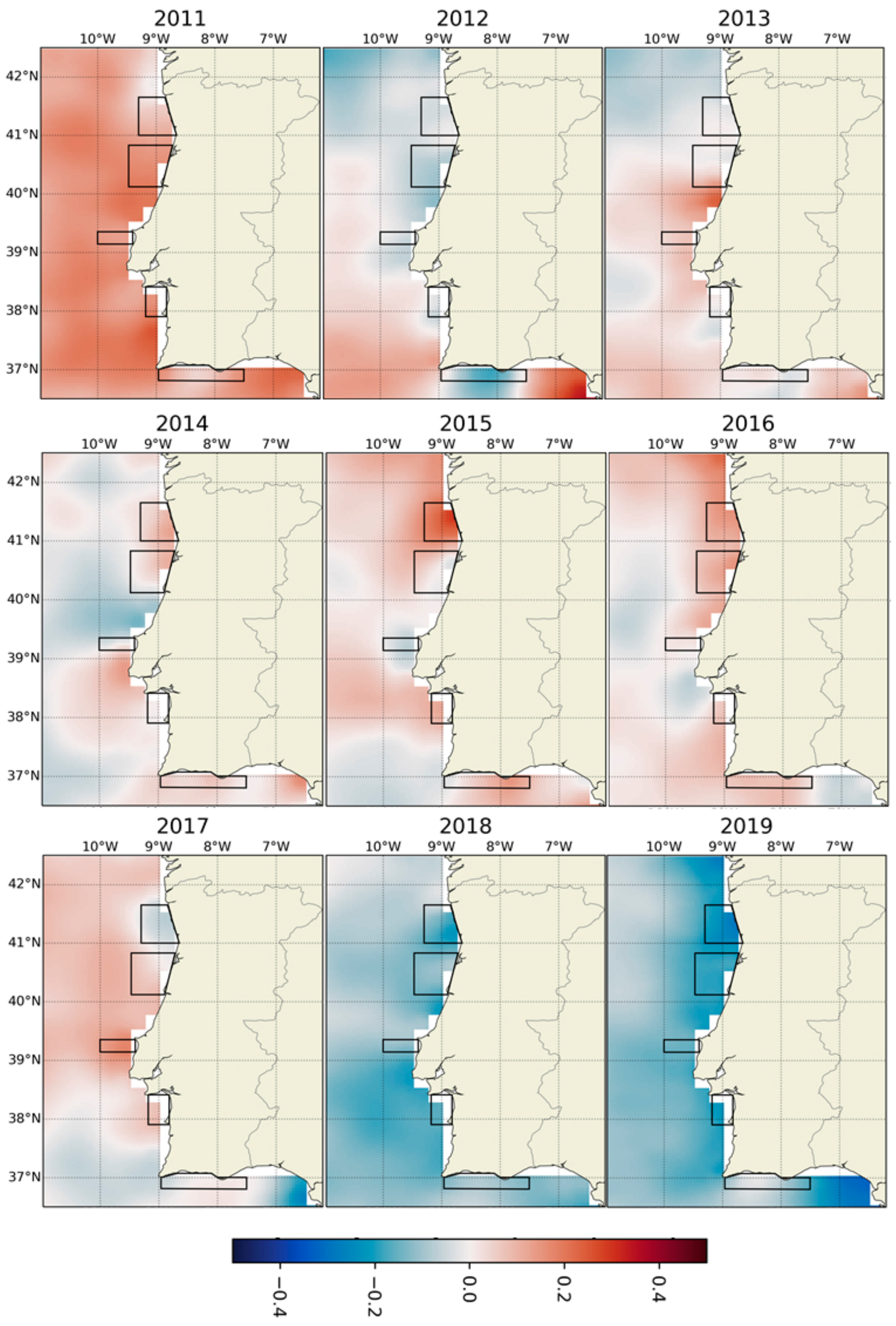
Yearly anomaly fields were calculated by subtracting the climatological SSS average (2011–2019) to the yearly average within each year from 2011 to 2019. Anomalies were also calculated for the periods of the conducted oceanographic cruises, again by subtracting the climatological SSS average for the corresponding period from the average SSS observed during the cruise. Therefore, for the Autumn 2018 cruise, for instance, spatial anomalies were determined by subtracting the SSS average in October 2011–2019 to the average in October 2018. For each pixel of the study site, the SSS linear trend for the entire dataset period was calculated, again by estimating the slope of the linear regression. To avoid potential missing values when deriving the trend, the resolution of the SSS dataset was first reduced to monthly averaged data.

Moreover, daily spatially averaged time series for the different regions (see the regions defined in Figure 1) were calculated, and statistical analysis was performed to assess the significance of the observed trends between 2011 and 2019. The statistical analysis was carried out considering linear regression parameters and the p value of the slope, significant if lower than 0.05 (95% confidence interval). Additionally, the Pettitt test was applied to determine the occurrence and timing of abrupt and significant changes in the mean of the time series [49,50]. This is one of the widely used tests for detecting changes in hydro-meteorological variables [50]. It uses the null hypothesis as the nonexistence of change in the data and the alternative hypothesis as the existence of change [51]. For a more detailed description of this method, see Li et al. 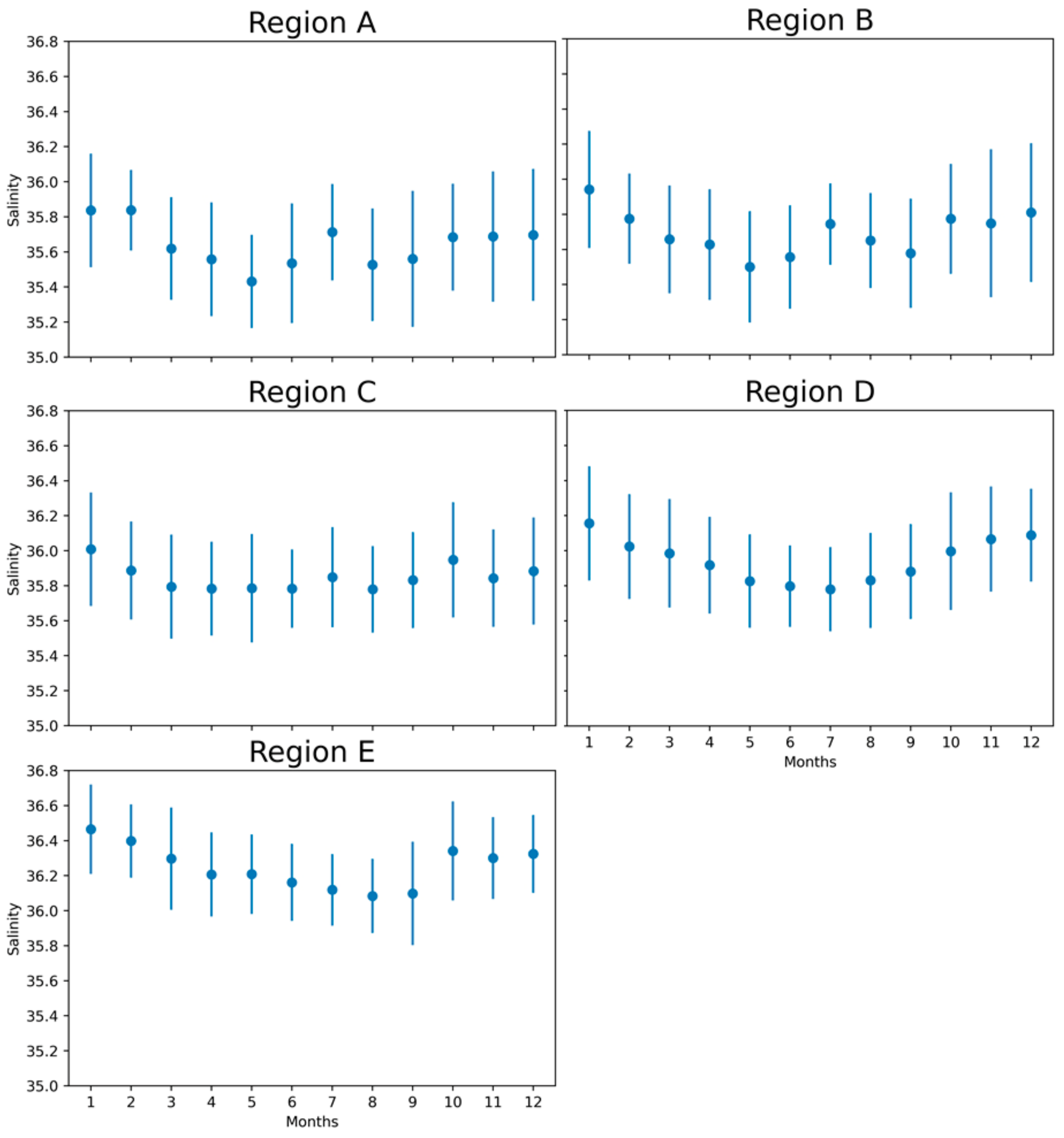[52]. The seasonal patterns were assessed by studying monthly averages (spatially averaged monthly means) for the different regions using the data from 2011 to 2019.

3. Results

3.1. Spatiotemporal Patterns of the Datasets

Satellite, modelled, and in situ datasets suggest that region E has the highest salinity values, revealing a north to south salinity gradient (Figure 2). Likewise, a coast-open ocean gradient with lower salinities on the coast was observed, especially in region A, although less evident with the in situ observations. However, within all regions, it was possible to detect discrepancies among the datasets obtained with satellite, modelled, and in situ observations (Figure 2). At first glance, the model seemed to deviate the most from the in situ observations and has a higher capability in retrieving salinity values near the coast. The satellite reveals serious limitations in presenting valid data for very coastal waters.

3.2. Matchup Analysis

The datasets were compared for each cruise (mentioned according to the season of the year) and colored according to the regions of study (Figure 3). It was possible to see that, for the three cruises, a good correlation between the satellite data and the in situ observations was obtained. The slope of the best-fitted line was close to 1, and the errors associated with the correlation (RMSE and bias) were less than 0.150 and 0.350 (in absolute value), respectively. Moreover, the R² was higher than 0.7 for the different cruises. The quality of the correlation between these two datasets, even if good, decreased slightly during Spring 2019 (Figure 3). On the other hand, the correlation between the in situ observations and the modelled data was not as good. Compared with the satellite, the model presented worse results in the matchup analysis (higher RMSE, bias, RPD and APD) (Figure 3).

During the cruise conducted in Autumn 2018, the satellite underestimated the salinities measured in regions A and B (with particular focus near the Douro region—Figure 2). The values of region E were also strongly underestimated for that period. During Spring 2019, the underestimation of the satellite was more evident in the whole A and B regions, but region A presented the highest differences between the datasets, mainly in its northern area (Figure 2 and Figure 3). On the other hand, during the Autumn 2019 cruise, there was a slight overestimation of the data in most of the regions A, B and E. Regarding the model, overall, there was an underestimation of the modelled data compared to the in situ observations (negative RPD, Figure 3), with an apparent increase in salinity with the increase of the distance to the coast (Figure 2). Particularly near the Mondego mouth, high differences between the model and the in situ data were observed during Autumn 2018 (Figure 2).

Considering a local scale, with a smaller range of salinity variation, satellite and modelled data were compared with the in situ observations for each studied region, with the matchups colored according to the sampling cruise (season) (Figure 4). The results for regions C and D should be viewed with caution as the number of matchups obtained with the satellite was lower than the ones of the remaining regions, especially in region D (only 21% of valid matchups were obtained, due to a particular lack of capacity of the satellite in accurately approaching to the coastal region in this zone). Overall, the model showed slightly worse results than the satellite. Exceptions were observed in region A and in regions C and D, where more matchups were identified for the model. Regarding the satellite data, region B showed the best results and, although it presented a lower R² than when the whole dataset was considered, it showed lower RMSE values (as all regions other than A). In all regions, there was a tendency for the satellite to underestimate the salinity values. This underestimation was even more evident with the model (negative RPD). The seasonal salinity variation was not clearly observed and seemed to worsen the data quality in regions A and E.

In order to have a better understanding of the regional differences between the datasets, the RPD (satellite/model—in situ) for each matchup was calculated, and the results were displayed in a map for better visualization (Figure 5 and Figure 6). Note that Figure 5 and Figure 6 do not have the same colour scale. Overall, the range of satellite RPD values was low, between −2.45 and 1.83% (average APD = 0.73% when considering the whole dataset). It was during the cruise conducted in Autumn 2019 that lower differences between the satellite and the in situ datasets were observed. In Spring 2019, the main differences were detected in region A, with a high underestimation of values by the satellite.

However, in some of the points sampled near shore during that cruise, a tendency for high overestimations was observed. On the other hand, the model RPD values achieved maximums of −9.31% (average APD = 1.49%). The worst results were obtained in the cruise conducted in Autumn 2018, with the highest values observed near the coast and mostly in Region A and B.

3.3. Error-Related Factors

The closer the measurements were to the coast, the higher APD values were detected (Figure 7). This pattern was more evident when considering the distance of the sampling points to the closest river of the Portuguese coast (Figure 7). This correlation was unclear in region E, where the highest APD (0.4%) was obtained between 20–30 km from the coast and the closest river. All those values were gathered in Autumn 2018. The depth at which the in situ surface values were measured (4 to 8 m) did not appear to have any bearing on the quality of the satellite product, suggesting a good mixture of the first meters of the water column (data not shown).

As for the water temperature, particularly during the cruise conducted in Spring 2019, the temperature variation was significantly related to the APD values, with higher APD associated with lower temperatures (Figure 8). Another source of error weighted with the present analysis focused on the variables involved in the satellite data generation. As mentioned above, the studied satellite product is a combination of SMOS salinity data with sea surface temperature data from the OSTIA program. As such, the relationship between the error values of the OSTIA product and the APD values from the concomitant satellite–in situ matchups was investigated. Overall, a tendency, significant albeit weak, to find higher values of APD associated with higher values of temperature errors was detected (Figure 9a). However, this relationship was only observed in the cruise conducted in Spring 2019 (as shown in Figure 9b), revealing some constraints regarding region A. When the different study regions were considered individually, region A showed a more prominent tendency to associate higher SST errors with higher APD, mainly due to data collected during Spring 2019. The data from region A (Figure 9c) is divided into two groups, with SST error values centered around 0.5 and 1.0, being this last group regarding coastal measurements. Therefore, the quality of the temperature data used appeared to have affected the quality of salinity data measured in region A during Spring 2019. The statistics obtained from the comparisons (by sampling cruise and study region) can be found in Table S1 from the Supplementary Materials.

3.4. Salinity Covariability with Biochemical Variables

In general terms, the RPD patterns observed in Figure 5 were not justified by the variability of any of the analyzed physicochemical and biological variables. Still, some exceptions were verified, mainly in the cruise conducted in Autumn 2019. The highest APD (absolute differences between satellite and in situ measurements) values in Region B were significantly associated (p value < 0.05) with higher values of turbidity (R² = 0.62) and SiO₂ (R² = 0.56) (Figure 10b,d). In region A, a weaker but significant correlation was perceived between higher APD and higher NO_x (R² = 0.23) and PO₄ (R² = 0.28) values (Figure 10a,c).

The satellite salinities were also compared with river flow data, but the lack of resolution of the product near the shore did not allow detecting a correlation between the parameters. Still, the satellite appeared to detect the presence of fresher water derived from large river discharges. However, this analysis will need further exploration as no good explanatory results were obtained.

3.5. Seasonal and Interannual Analysis

The satellite product allowed a study of interannual variations of the sea surface salinity along the Portuguese coast. The calculated salinity anomalies presented different patterns since 2011 (Figure 11). 2011 was the year with the highest anomalies detected within the 2011–2019 study period, and it was the only year that showed overall positive anomalies along the coast. In contrast, 2018 and 2019 showed the opposite pattern, with negative anomalies throughout the area under analysis. 2017–2018 appeared to be the period when the change of the salinity signal occurred (Figure 11). This observation was confirmed with the Pettitt test (change-point detection), which detected a significantly probable shift point in the first months of 2017 (for regions A, D, and E) and 2018 (for regions B and C), using the spatially averaged time series gathered for the five studied regions (Figure 12). The time series analysis (Figure 12), besides presenting the spatial pattern previously detected, showed a statistically significant decreasing trend of the sea surface salinity along almost the coastal region of Portugal since 2011. This trend appeared to be more evident after 2017 and can be seen in Figure 11. Region E did not present statistically significant monthly trends for most of its area, similar to the observations in the coastal ocean near Galicia.

Along with the interannual analysis, the seasonal salinity variation was studied for the different regions (Figure 13). Higher salinity values were observed during the winter months along the coast. However, comparing the regions, the lowest values were detected at different times of the year. Region A presented a tendency for a decrease of salinity during spring, followed by a peak in July. This peak is observed to weaken towards the south and is no longer observed at region D. Both in regions D and E, the lowest salinities tended to be observed during the summer months. Region E was divided into two subareas (the western and eastern sections) due to the different circulation regimes characteristic of the area and showed slightly different patterns along the coast (Figure 14). The seasonal pattern observed in the western part of region E presented the highest similarities to the variability observed in the northwest coast of Portugal, with a slight salinity peak detected in July.

4. Discussion

Previous studies involving the quantification of salinity by satellite suggest the need to continue investing in this type of analysis in coastal regions to reach satisfactory results when comparing the satellite-derived data and in situ observations (e.g., [10,17]). The present analysis is no exception, as the satellite quantification of salinity remains difficult in these near-shore dynamic systems. Nevertheless, significant progress was accomplished with the application of the L4 product from SMOS in the coastal region of Portugal. Compared with the existing literature, such as [12,53], the satellite product presented satisfying results in retrieving surface salinity in a coastal region. It also presented better performance than the hydrodynamic model, despite the model’s increased capacity to provide data near the coastline. These results suggest that the assimilation of satellite salinity data by the model can help improve and better understand the dynamics in this region.

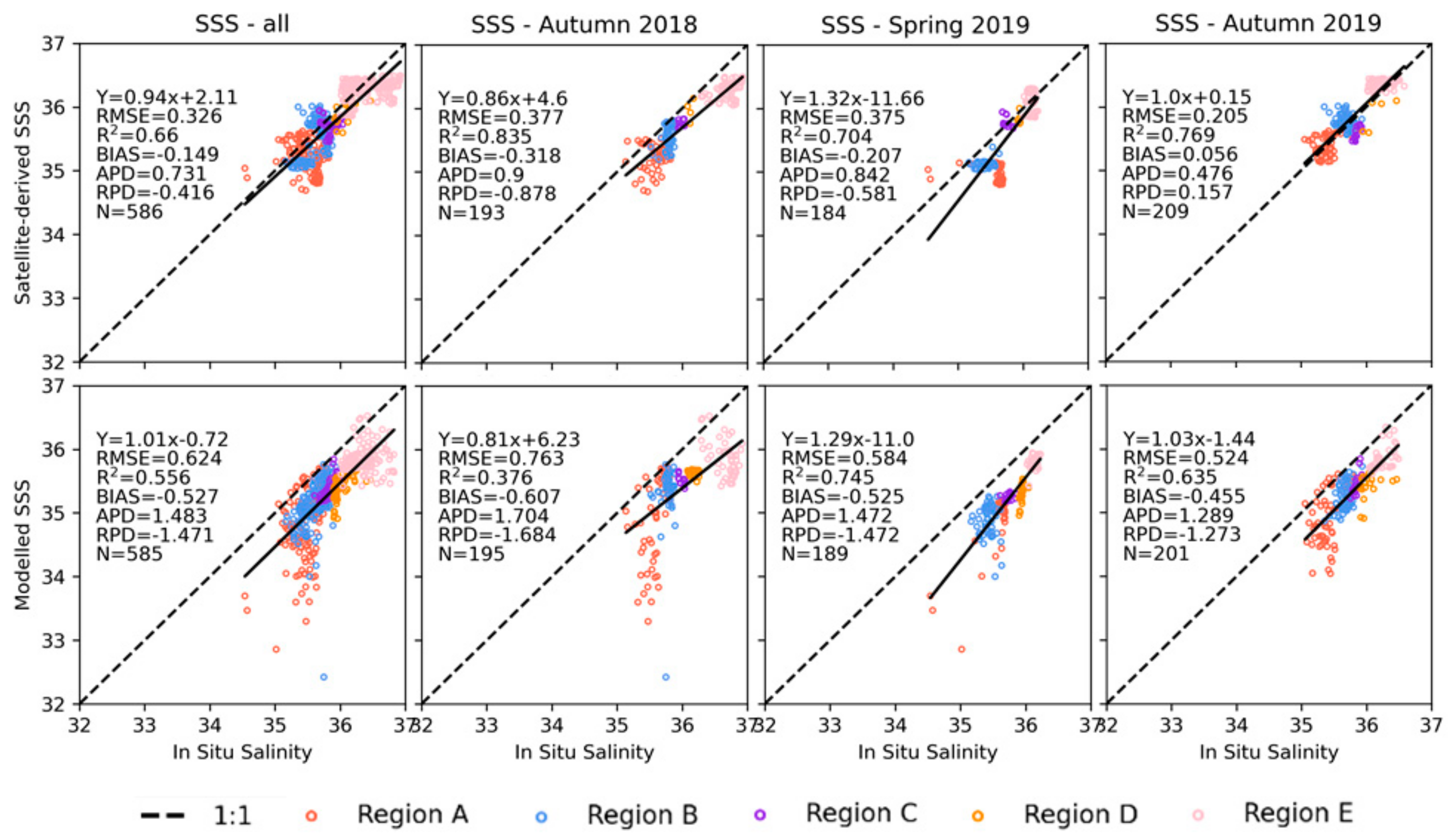
According to Köhl et al. [54], typical error amplitudes in coastal regions reside between 1 and 2 units. During this study, the difference between satellite and in situ measurements never exceeded 1 unit (mean bias of −0.149), with an average RMSE of 0.326 and a mean APD of 0.73%. Following Jorge Vazquez–Cuervo et al. [17], the signal-to-noise ratio was calculated and, using the whole dataset, a value of 1.52 was obtained. This value was equivalent to the signal-to-noise obtained by Jorge Vazquez-Cuervo et al. [17] with a SMOS L3 product around 50 km, highlighting the improvement achieved with the L4 SMOS SSS product in quantifying coastal salinities. The obtained statistical set confirms the accuracy of the satellite measurements, validating the quality of the product. However, caution must be taken when analyzing the RPD and APD since these are relative measures. A 0.73% deviation from the mean in situ value (35.90) results in a difference between the datasets of 0.26 units, which corresponds to a high error when framed in the seasonal variability range (around 0.40). Overall, the results of this analysis could be seen as complementary to the work developed by The Pilot-Mission Exploitation Platform (Pi-MEP) [14].

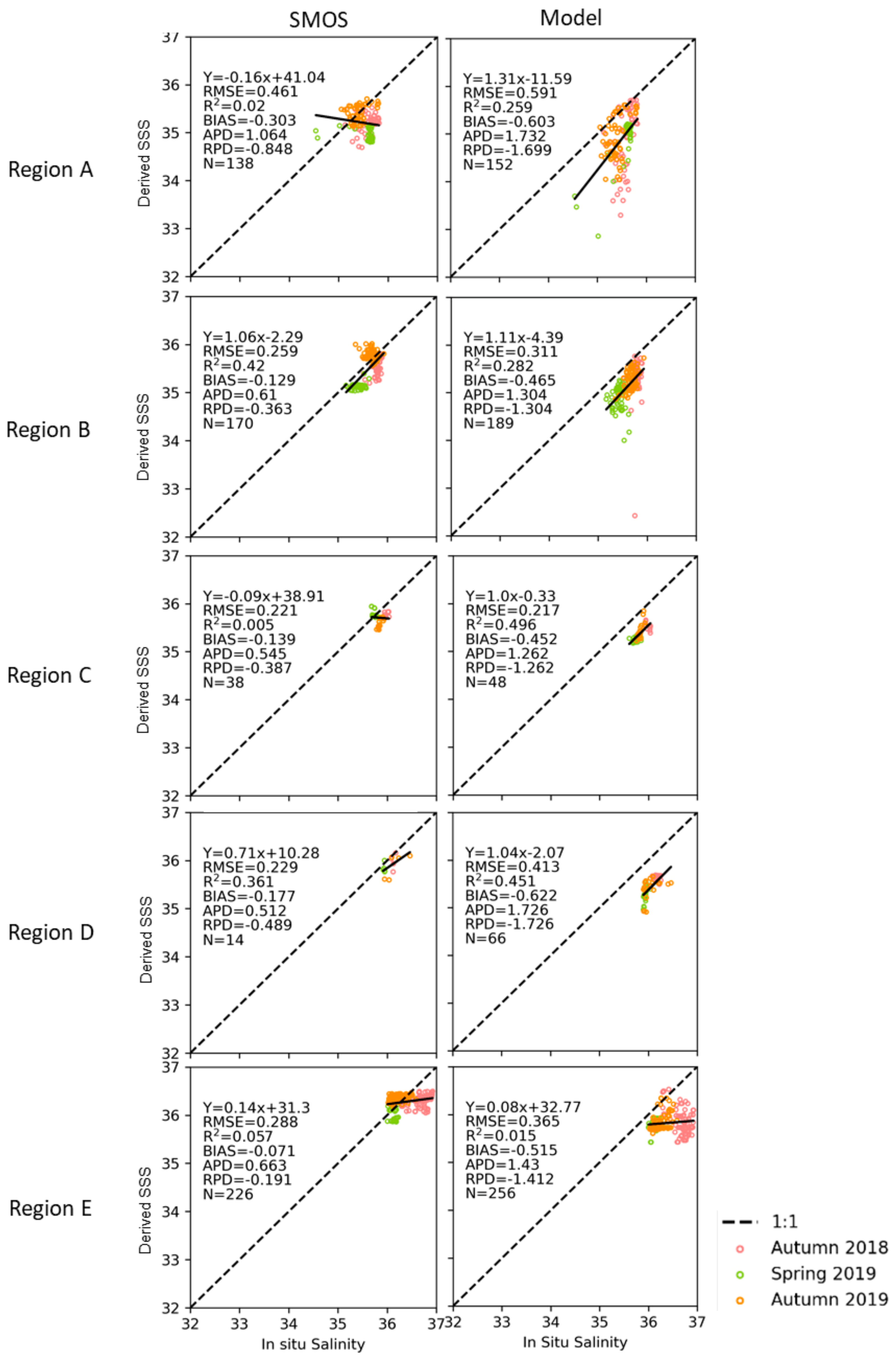
Despite the overall quality of the satellite data, its comparison with the in situ observations presented slightly worse results when each study region was considered individually. The satellite showed limitations in accurately capturing smaller salinity ranges, more critically in regions A and E. In addition, the product was not able to retrieve salinity data similarly along the coast: in region E, south coast of Portugal, the product obtained valid data close to 2 km off the shoreline, while in region D (southwest of Portugal), only data measured from 13 km off the coastline obtained valid data. Note that the expected effective spatial resolution of this satellite L4 product is around 20 km. The results presented in this study showed good performance in all the regions up to 20 km, which is consistent with the expected effective spatial resolution of the product. Closer than 20 km, the product presents extrapolated salinity values, and the results must be considered with some caution. Still, as tested, the extrapolated values were observed to be of good quality and could be a valuable tool to surpass the common coastal measurements, which in the literature usually refer to data obtained 40 km off the coast [10,11,55] (Figure 5).

Besides land contamination, regionally, SMOS coastal salinity retrievals could also be influenced by high levels of radio frequency interference (RFI) [11,16]. These two factors interfere with the brightness temperature acquisition posing limitations on obtaining quality salinity retrievals near land [18] and could justify the higher errors obtained near the coast during the present study. 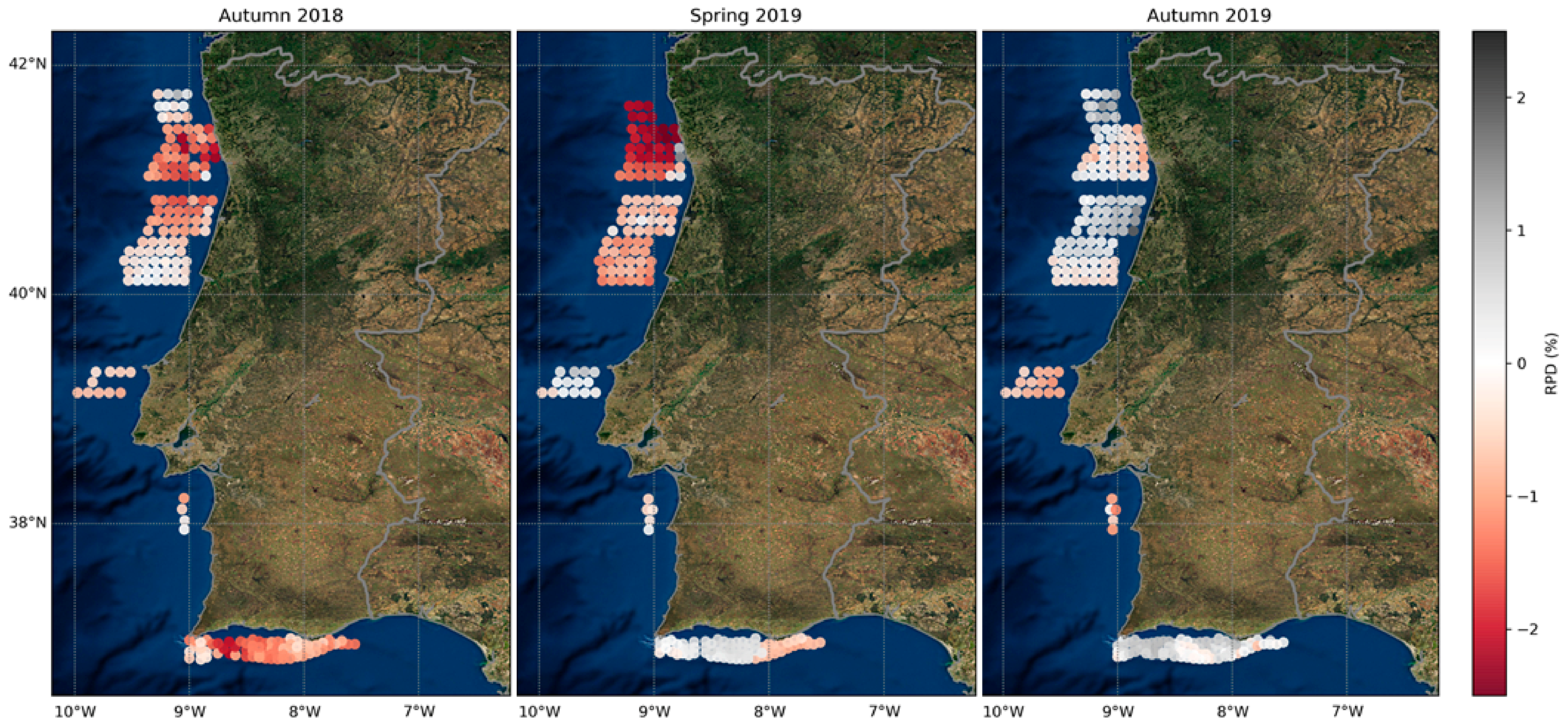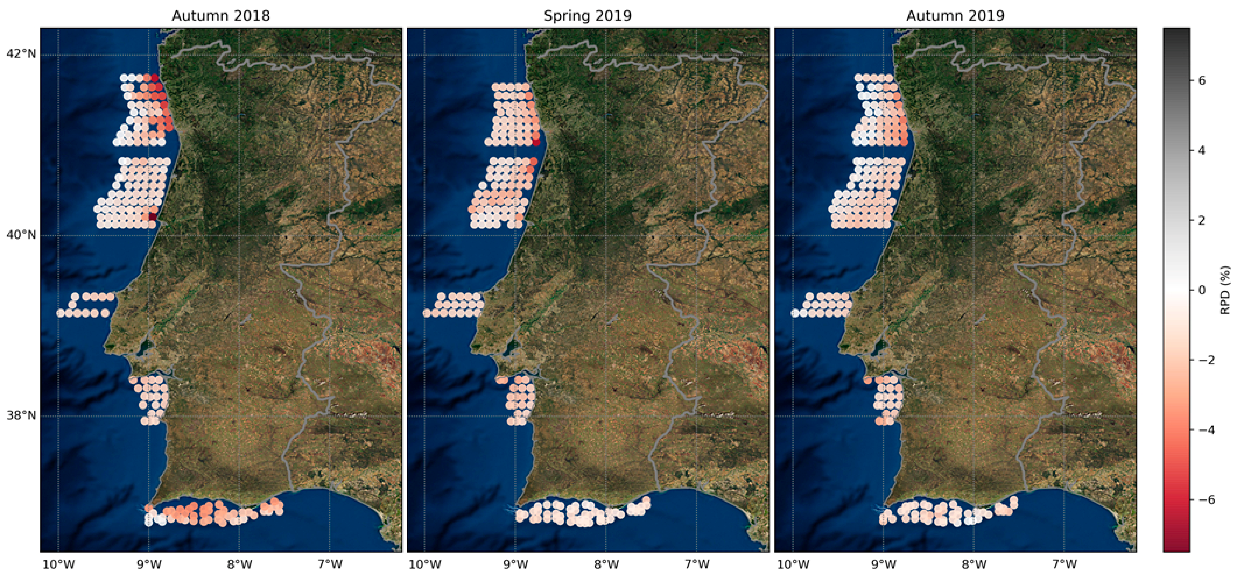Therefore, continuing to support the improvement of the RFI detection and geolocation algorithms [18] will help mitigate this situation. On the other hand, region E showed a different pattern, with higher RPD values associated with measurements between 20 to 30 km from the coast (data referring to Autumn 2018). It is possible that this finding resulted from particularly high in situ salinity values observed in that region during the days in which that cruise was conducted (when compared with the same period of the following year), leading to the satellite underestimation of the data. Nevertheless, the satellite should have been able to detect these higher values, suggesting there may exist some constraints on the product characteristics, currently not easily detectable.

Another factor that influenced the overall quality of the product was the distance of the measurements to rivers. The analysis suggests that the satellite has more significant constraints in quantifying salinity near regions influenced by Portuguese freshwater river plumes (small river plumes). This is probably because their presence increases the dynamic of the region, causing stronger spatial variability in a reduced area. It is also possible that this observation reveals a residual land–sea contamination in the satellite measurements or results from the differences between the spatial and temporal scales of the datasets being compared. Another factor that could highlight the constraints in quantifying salinity near river plumes is the correlation observed between high values of APD and high values of turbidity and silicate in some campaigns. This could indicate a worse performance of the product under the influence of land runoff, rain, or higher river flow. As for the performance of the product under the influence of other oceanographic/environmental processes, such as upwelling, it was not possible to reach concrete conclusions. Further investigation is still needed.

The fact that the in situ measurements were taken a few meters below the surface was also carefully weighed [14] against the fact that the satellite retrieves data from the top 0.5–1 cm of the ocean surface. 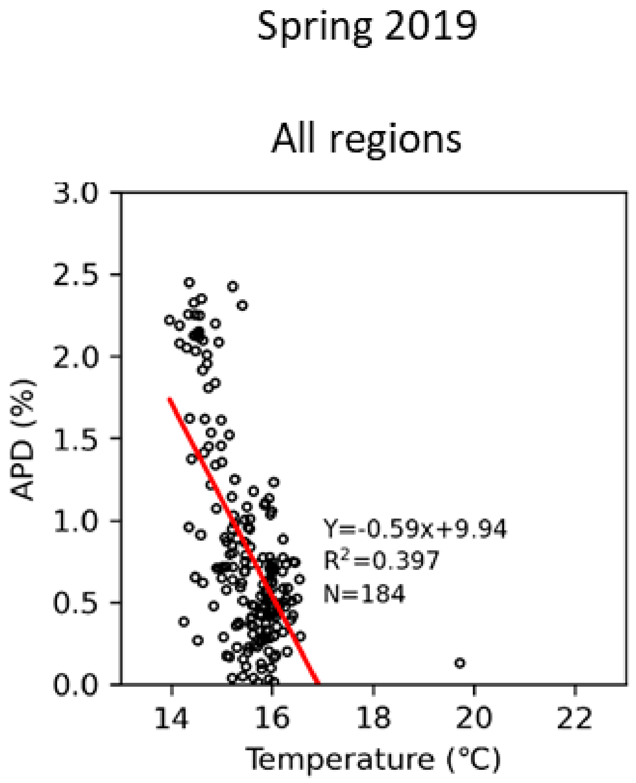Accordingly, it was perceived that higher errors were not associated with higher measurement depths, thus, using data gathered between 4 and 8 m depth as surface values did not increase the differences between in situ and satellite measurements when considering this product. Moreover, higher APD values were associated with lower temperatures, particularly during the cruise conducted in Spring 2019. This observation was somewhat expected as the sensitivity of the L-band brightness temperatures to the salinity decreases as the sea surface temperature decreases. However, the most significant quality degradation occurs at SST values lower than 10 °C [56], which is lower than the SST range of values observed in the present study.

Despite the factors that affected the quality of the measurements at a regional scale, the product was able to adequately perceive spatial patterns along the Portuguese coast, even when considering short-term periods. The region of the country’s south coast (Region E) was characterized by having higher salinity values through the year than region A (northwest coast), which presented the lower values. These results are corroborated in previous studies by Moita [57] and Campuzano et al. [58] and arise from higher rates of evaporation–precipitation in the south of Portugal compared with the north [59,60].

Seasonally, it was possible to see that winter months presented higher salinity values along the Portuguese coast. This observation is supported by the presence of the Iberian Poleward Current that carries warmer and saltier waters from the south [25], although offshore, the pattern is the opposite, as shown in the NOAA World Ocean Atlas 2018 [61] based on seasonal averages of data gathered between 1981 and 2010. During spring and summer, the west coast of Portugal is influenced by upwelling [24,27]. Over the continental shelf and slope of the WIC, the upwelling regime promotes an alongshore equatorward surface current that carries cooler and less salty water, in accordance with the southward gradient of surface salinity identified in Figure 2. This behavior is corroborated by the monthly analysis conducted that showed a decrease of salinity values during the spring and summer months in all regions. However, a peak in salinity was observed in July, more prominently in the northwest region of the country (regions A and B). A similar pattern was also observed by Taylor and Stephens [62] in their station K (station on the North Atlantic coast, near the WIC). The authors explained the observed seasonal variation as a consequence of seasonal variations of evaporation and precipitation (minimum evaporation–precipitation obtained during summer). Therefore, the monthly variability detected in the present study could be the result of the combination of seasonal upwelling and evaporation–precipitation rates. However, further studies are needed to understand these regional variations fully.

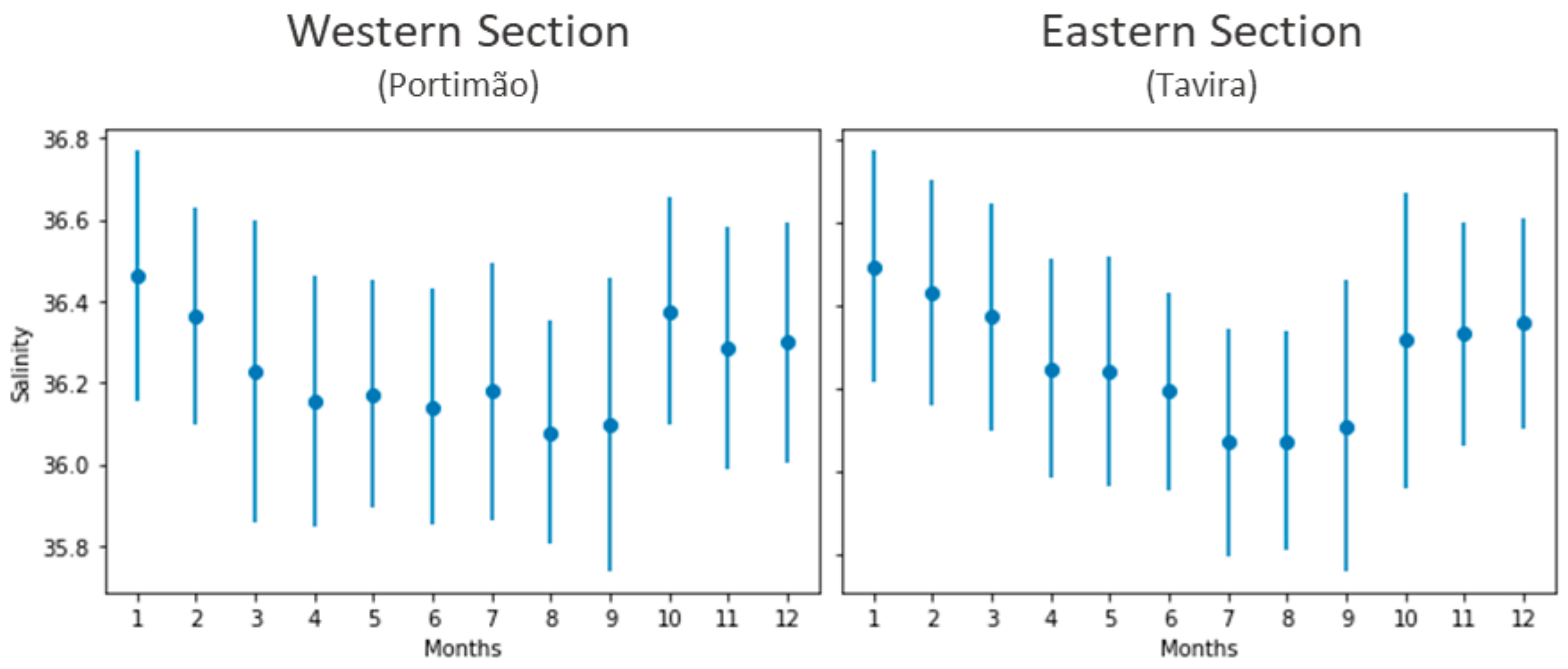
Coastal upwelling affects the south coast of Portugal differently. Analyzing the salinity variability in the two regions separated by Cape Santa Maria (western and eastern sections of region E), it was possible to see slightly different patterns. The variability observed in the western section was more similar to the variability observed in the west coast of Portugal. As noted by García-Lafuente et al. [28], during spring-summer, the Cape Santa Maria (see Figure S1) separates the surface circulation over the continental shelf, and the western cell is influenced by the seasonal upwelling that occurs on the west coast of the country, i.e., the intrusion of the coastal upwelling jet from the west coast of Portugal with colder and less salty water [29]. The seasonal variability observed in Region E during winter was possibly derived mainly by a coastal current directed to the west in the western cell and the east in the eastern section [29]. Both currents fed by water transport from the inland Gulf of Cadiz, unaffected by freshwater runoff from the main rivers. The patterns observed with the satellite images also confirm that during winter, the main Portuguese rivers do not have a high flow necessary to reduce the salinity near the coast (higher salinities detected during the winter months). The study of the main river plumes using the L4 SMOS SSS remains challenging, given its spatial resolution.

Analyzing the SMOS SSS data, it was possible to detect a significant decreasing trend in water salinity between 2011 and 2019, almost along the entire Portuguese coast. A decreasing salinity trend was previously observed in several areas of the North Atlantic Ocean (e.g., [63,64]) and could have been enhanced by changes in freshwater fluxes and subpolar gyre circulation, with slowing of the North Atlantic Current and diversion of Arctic freshwater from the western boundary into the eastern basins [65]. Changes in regional air–sea fluxes in near coastal regions may also be an additional factor contributing to the decreasing salinity trend [25]. The studied time series is short for long-term analysis; thus, it is not easy to conclude the origin of this decrease. Further investigations of this phenomenon are needed and will constitute future work. Still, the interannual and seasonal analysis reveals a high regional and global relevance. First, on the regional level, no studies focused on the salinity patterns along the WIC coast (or this region of the Atlantic) were ever published using this spatial coverage and temporal resolution, and little is known about the topic. Second, globally, it is now possible to use a decade of global high resolution and high-quality salinity data obtained from space—quality proved throughout the present study—for climatological studies, coastal dynamic, and short-term event analyses near the coast, that will enhance our knowledge of coastal circulation and ocean–atmosphere interactions.

5. Conclusions

The present study aimed to test the usefulness of the BEC SMOS L4 Sea Surface Salinity product for the region of the Portuguese coast, aspiring to future applications in climatological, coastal dynamic and short-term event analysis.

Satisfactory results were obtained in the comparison of the satellite-derived salinity and the in situ observations. Overall, the range of RPD values obtained was low, as the other errors associated, contrasting with high R². It was possible to conclude that this product has a high potential for coastal climatological research, being a high-quality product for long-term analysis on the Iberian coast. This product can be considered a reliable complement to in situ measurements, and it was demonstrated to provide more valuable and complementary information than the existing hydrographic models. Still, some limitations were detected, mainly in quantifying salinity values near the coastline of Portugal (with more significant evidence on the southwest coast). The proximity to the coast and the mouth of the rivers were the factors that most influenced the quality of the product. The assimilation of satellite data by the model could provide new insight into these coastal regions. The depth of the in situ measurements considered did not appear to correlate to higher RPD values. Thus, it is possible to conclude that using measurements gathered between 4 and 8 m depth as surface values does not introduce errors into the analysis when considering this product. High errors of the satellite temperature data used in the production of the dataset (>0.5 °C) also influenced the product quality assessment and should be carefully evaluated in creating future salinity products.

In the future, it would be interesting and rewarding to study the regional, seasonal variability of evaporation–precipitations rates, as well as the upwelling events, to clearly understand the seasonal salinity patterns observed during this analysis along the Portuguese coast. The relationship between satellite salinities and river flow data will need to be further explored, and further investigations on the salinity trends observed will constitute future work within the climate change framework, preferably with longer SSS time series. The present analysis allows us to confirm the validity of using satellite salinity data in analyzing coastal regions, and thus, can be considered a relevant contribution to the global studies of coastal dynamics and short-term events. It also proves that it is important to continue to support the development of new products, building long time series and with a better spatial resolution, so that the coastal ocean, and possibly estuaries, essential environmental indicators of climate change, can start being studied confidently using these cost-effective tools.

References

1. Klemas, V. Remote Sensing of Sea Surface Salinity: An Overview with Case Studies. J. Coast. Res. 2011, 27, 830–838. [Google Scholar] [CrossRef]
2. NASA—With a Pinch of Salt. Available online: https://climate.nasa.gov/news/58/with-a-pinch-of-salt/ (accessed on 16 September 2021).
3. Talley, L.D.; Pickard, G.L.; Emery, W.J.; Swift, J.H. Descriptive Physical Oceanography. An Introduction, 6th ed.; Elsevier Ltd.: Amsterdam, The Netherlands, 2011; ISBN 9780750645522. [Google Scholar]
4. Jain, C.K. Salinity. In Encyclopedia of Snow, Ice and Glaciers; Singh, V.P., Singh, P., Haritashya, U.K., Eds.; Springer: Dordrecht, The Netherlands, 2011; p. 959. ISBN 978-90-481-2642-2. [Google Scholar]
5. Fedorov, A.V.; Pacanowski, R.C.; Philander, S.G.; Boccaletti, G. The effect of salinity on the wind-driven circulation and the thermal structure of the upper ocean. J. Phys. Oceanogr. 2004, 34, 1949–1966. [Google Scholar] [CrossRef] [Green Version]
6. Durack, P.J.; Lee, T.; Vinogradova, N.T.; Stammer, D. Keeping the lights on for global ocean salinity observation. Nat. Clim. Chang. 2016, 6, 228–231. [Google Scholar] [CrossRef]
7. ESA—New Maps of Salinity Reveal the Impact of Climate Variability on Oceans. Available online: https://esa.int/Applications/Observing_the_Earth/Space_for_our_climate/New_maps_of_salinity_reveal_the_impact_of_climate_variability_on_oceans (accessed on 17 September 2021).
8. Lagerloef, G.S.E.; Swift, C.T.; Le Vine, D.M. Sea Surface Salinity: The Next Remote Sensing Challenge. Oceanography 1995, 8, 44–50. [Google Scholar] [CrossRef]
9. Font, J.; Camps, A.; Borges, A.; Martín-Neira, M.; Boutin, J.; Reul, N.; Kerr, Y.H.; Hahne, A.; Mecklenburg, S. SMOS: The Challenging Sea Surface Salinity Measurement from Space. Proc. IEEE 2010, 98, 649–665. [Google Scholar] [CrossRef] [Green Version]
10. Vinogradova, N.; Lee, T.; Boutin, J.; Drushka, K.; Fournier, S.; Sabia, R.; Stammer, D.; Bayler, E.; Reul, N.; Gordon, A.; et al. Satellite Salinity Observing System: Recent Discoveries and the Way Forward. Front. Mar. Sci. 2019, 6, 243. [Google Scholar] [CrossRef]
11. Reul, N.; Grodsky, S.A.; Arias, M.; Boutin, J.; Catany, R.; Chapron, B.; D’Amico, F.; Dinnat, E.; Donlon, C.; Fore, A.; et al. Sea surface salinity estimates from spaceborne L-band radiometers: An overview of the first decade of observation (2010–2019). Remote Sens. Environ. 2020, 242, 111769. [Google Scholar] [CrossRef]
12. Bao, S.; Wang, H.; Zhang, R.; Yan, H.; Chen, J. Comparison of Satellite-Derived Sea Surface Salinity Products from SMOS, Aquarius, and SMAP. J. Geophys Res. Ocean. 2019, 124, 1932–1944. [Google Scholar] [CrossRef]
13. Stammer, D.; Martins, M.S.; Köhler, J.; Köhl, A. How well do we know ocean salinity and its changes? Prog. Oceanogr. 2021, 190, 102478. [Google Scholar] [CrossRef]
14. Guimbard, S.; Reul, N.; Sabia, R.; Herlédan, S.; Hanna, Z.E.K.; Piollé, J.F.; Paul, F.; Lee, T.; Schanze, J.J.; Bingham, F.M.; et al. The salinity pilot-mission exploitation platform (Pi-mep): A hub for validation and exploitation of satellite sea surface salinity data. Remote Sens. 2021, 13, 4600. [Google Scholar] [CrossRef]
15. Olmedo, E.; Campuzano, F.; Turiel, A.; Oliveira, P.B.; Angélico, M.M. SMOS Sea Surface Salinity contribution to the Land-Marine Boundary Development and Analysis (LAMBDA) project. In Proceedings of the Atlantic form Space Workshop, Southampton, UK, 23–25 January 2019; pp. 44–45. [Google Scholar]
16. Grodsky, S.A.; Reul, N.; Bentamy, A.; Vandemark, D.; Guimbard, S. Eastern Mediterranean salinification observed in satellite salinity from SMAP mission. J. Mar. Syst. 2019, 198, 103190. [Google Scholar] [CrossRef]
17. Vazquez-Cuervo, J.; Gomez-Valdes, J.; Bouali, M.; Miranda, L.E.; Van der Stocken, T.; Tang, W.; Gentemann, C. Using saildrones to validate satellite-derived sea surface salinity and sea surface temperature along the California/Baja coast. Remote Sens. 2019, 11, 1964. [Google Scholar] [CrossRef] [Green Version]
18. González-Gambau, V.; Olmedo, E.; Martínez, J.; Turiel, A.; Durán, I. Improvements on Calibration and Image Reconstruction of SMOS for Salinity Retrievals in Coastal Regions. IEEE J. Sel. Top. Appl. Earth Obs. Remote Sens. 2017, 10, 3064–3078. [Google Scholar] [CrossRef]
19. Akter, R.; Asik, T.Z.; Sakib, M.; Akter, M.; Sakib, M.N.; Al Azad, A.S.M.A.; Maruf, M.; Haque, A.; Rahman, M.M. The Dominant Climate Change Event for Salinity Intrusion in the GBM Delta. Climate 2019, 7, 69. [Google Scholar] [CrossRef] [Green Version]
20. Sotillo, M.G.; Campuzano, F.; Guihou, K.; Lorente, P.; Olmedo, E.; Matulka, A.; Santos, F.; Amo-Baladrón, M.A.; Novellino, A. River freshwater contribution in operational ocean models along the european atlantic façade: Impact of a new river discharge forcing data on the cmems ibi regional model solution. J. Mar. Sci. Eng. 2021, 9, 401. [Google Scholar] [CrossRef]
21. Baladrón, A.A.; Levier, B.; Sotillo, M.G. Product User Manual for Atlantic-Iberian Biscay Irish-Ocean Physics Reanalysis Product IBI_MULTIYEAR_PHY_005_002. Copernicus Marine Service, September 2020. Available online: https://resources.marine.copernicus.eu/product-detail/IBI_MULTIYEAR_PHY_005_002/INFORMATION (accessed on 25 October 2021).
22. Olmedo, E.; González-Haro, C.; Hoareau, N.; Umbert, M.; Gambau, V.G.; Martínez, J.; Gabarró, C.; Turiel, A. Nine years of SMOS sea surface salinity global maps at the Barcelona Expert Center. Earth Syst. Sci. Data 2021, 13, 857–888. [Google Scholar] [CrossRef]
23. Mantas, V.M.; Pereira, A.J.S.C.; Marques, J.C. Partitioning the ocean using dense time series of Earth Observation data. Regions and natural boundaries in the Western Iberian Peninsula. Ecol. Indic. 2019, 103, 9–21. [Google Scholar] [CrossRef]
24. Relvas, P.; Barton, E.D.; Dubert, J.; Oliveira, P.B.; Peliz, Á.; da Silva, J.C.B.; Santos, A.M.P. Physical oceanography of the western Iberia ecosystem: Latest views and challenges. Prog. Oceanogr. 2007, 74, 149–173. [Google Scholar] [CrossRef] [Green Version]
25. Teles-Machado, A.; Peliz, A.; McWilliams, J.C.; Cardoso, R.M.; Soares, P.M.M.; Miranda, P.M.A. On the year-to-year changes of the Iberian Poleward Current. J. Geophys. Res. Ocean 2015, 120, 4980–4999. [Google Scholar] [CrossRef]
26. Peliz, Á.; Rosa, T.L.; Santos, A.M.P.; Pissarra, J.L. Fronts, jets, and counter-flows in the Western Iberian upwelling system. J. Mar. Syst. 2002, 35, 61–77. [Google Scholar] [CrossRef]
27. Sousa, M.C.; deCastro, M.; Alvarez, I.; Gomez-Gesteira, M.; Dias, J.M. Why coastal upwelling is expected to increase along the western Iberian Peninsula over the next century? Sci. Total Environ. 2017, 592, 243–251. [Google Scholar] [CrossRef] [PubMed]
28. García-Lafuente, J.; Delgado, J.; Criado-Aldeanueva, F.; Bruno, M.; del Río, J.; Miguel Vargas, J. Water mass circulation on the continental shelf of the Gulf of Cádiz. Deep Res. Part II Top. Stud. Oceanogr. 2006, 53, 1182–1197. [Google Scholar] [CrossRef]
29. Criado-Aldeanueva, F.; Garcia-Lafuente, J.; Navarro, G.; Ruiz, J. Seasonal and interannual variability of the surface circulation in the eastern Gulf of Cadiz (SW Iberia). J. Geophys. Res. Ocean 2009, 114. [Google Scholar] [CrossRef] [Green Version]
30. Peliz, Á.; Dubert, J.; Santos, A.M.P.; Oliveira, P.B.; Le Cann, B. Winter upper ocean circulation in the Western Iberian Basin—Fronts, Eddies and Poleward Flows: An overview. Deep Res. Part I Oceanogr. Res. Pap. 2005, 52, 621–646. [Google Scholar] [CrossRef]
31. Sánchez, R.F.; Relvas, P.; Delgado, M. Coupled ocean wind and sea surface temperature patterns off the western Iberian Peninsula. J. Mar. Syst. 2007, 68, 103–127. [Google Scholar] [CrossRef]
32. IPMA—E em Portugal O Clima Está a Mudar? Available online: https://www.ipma.pt/pt/educativa/faq/climatologia/faqdetail.html?f=/pt/educativa/faq/climatologia/faq_0004.html (accessed on 23 September 2021).
33. IPMA—Clima de Portugal Continental. Available online: https://www.ipma.pt/pt/educativa/tempo.clima/index.jsp?page=clima.pt.xml (accessed on 26 August 2021).
34. Campuzano, F.; Santos, F.; Ramos de Oliveira, A.I.; Simionesei, L.; Fernandes, R.; Brito, D.; Olmedo, E.; Turiel, A.; Alba, M.; Novellino, A.; et al. Framework for improving land boundary conditions in regional ocean products. In Proceedings of the EGU General Assembly, Online, 4–8 May 2020. [Google Scholar]
35. Umbert, M.; Hoareau, N.; Turiel, A.; Ballabrera-Poy, J. New blending algorithm to synergize ocean variables: The case of SMOS sea surface salinity maps. Remote Sens. Environ. 2014, 146, 172–187. [Google Scholar] [CrossRef]
36. Turiel, A.; Yahia, H.; Pérez-Vicente, C.J. Microcanonical multifractal formalism—A geometrical approach to multifractal systems: Part I. Singularity analysis. J. Phys. A Math. Theor. 2007, 41, 15501. [Google Scholar] [CrossRef]
37. Isern-Fontanet, J.; Turiel, A.; García-Ladona, E.; Font, J. Microcanonical multifractal formalism: Application to the estimation of ocean surface velocities. J. Geophys Res. Ocean 2007, 112, 1–18. [Google Scholar] [CrossRef] [Green Version]
38. Nieves, V.; Llebot, C.; Turiel, A.; Solé, J.; García-Ladona, E.; Estrada, M.; Blasco, D. Common turbulent signature in sea surface temperature and chlorophyll maps. Geophys. Res. Lett. 2007, 34, 1–5. [Google Scholar] [CrossRef] [Green Version]
39. Olmedo, E.; Martínez, J.; Umbert, M.; Hoareau, N.; Portabella, M.; Ballabrera-Poy, J.; Turiel, A. Improving time and space resolution of SMOS salinity maps using multifractal fusion. Remote Sens. Environ. 2016, 180, 246–263. [Google Scholar] [CrossRef]
40. González-Gambau, V.; Turiel, A.; González-Haro, C.; Martínez, J.; Olmedo, E.; Oliva, R.; Martín-Neira, M. Triple collocation analysis for two error-correlated datasets: Application to l-band brightness temperatures over land. Remote Sens. 2020, 12, 3381. [Google Scholar] [CrossRef]
41. Hoareau, N.; Turiel, A.; Portabella, M.; Ballabrera-Poy, J.; Vogelzang, J. Singularity Power Spectra: A Method to Assess Geophysical Consistency of Gridded Products—Application to Sea-Surface Salinity Remote Sensing Maps. IEEE Trans. Geosci. Remote Sens. 2018, 56, 5525–5536. [Google Scholar] [CrossRef] [Green Version]
42. Sá, C.; D’Alimonte, D.; Brito, A.C.; Kajiyama, T.; Mendes, C.R.; Vitorino, J.; Oliveira, P.B.; da Silva, J.C.B.; Brotas, V. Validation of standard and alternative satellite ocean-color chlorophyll products off Western Iberia. Remote Sens. Environ. 2015, 168, 403–419. [Google Scholar] [CrossRef]
43. Martin, M.; Fiedler, E.; Roberts-Jones, J.; Blockley, E.; McLaren, A.; Good, S. Product User Manual for OSTIA Near Real Time Level 4 SST Products over the Global Ocean SST-GLO-SST-L4-NRT-OBSERVATIONS-010-001. Copernicus Marine Environment Monitoring Service, 22 March 2019. Available online: https://cupdf.com/document/product-user-manual-for-ostia-near-real-time-level-4-sst-product-user-manual.html (accessed on 25 October 2021).
44. UK Met Office. OSTIA L4 SST Analysis (GDS2). Ver. 2.0; PO.DAAC: Pasadena, CA, USA, 2012. Available online: https://doi.org/10.5067/GHOST-4FK02 (accessed on 27 September 2021).
45. Strickland, J.; Parsons, T. A Practical Handbook of Seawater Analysis. Fish. Res. Board Can. Ott. Bull. 1972, 167, 328. [Google Scholar]
46. Murphy, J.; Riley, J. A modified single solution method for the determination of phosphate in natural waters. Anal. Chim. Acta 1962, 27, 31–36. [Google Scholar] [CrossRef]
47. Aminot, A.; Rey, F. Chlorophyll a: Determination by spectroscopic methods. ICES Tech. Mar. Environ. Sci. 2001, 30, 17. [Google Scholar] [CrossRef]
48. Jeffrey, S.W.; Humphrey, G.F. New spectrophotometric equations for determining chlorophylls a, b, c1 and c2 in higher plants, algae and natural phytoplankton. Biochem Physiol. Pflanz. 1975, 167, 191–194. [Google Scholar] [CrossRef]
49. Pettitt, A.N. A Non-Parametric Approach to the Change-Point Problem. J. R Stat. Soc. Ser. C (Appl. Stat.) 1979, 28, 126–135. [Google Scholar] [CrossRef]
50. Serinaldi, F.; Kilsby, C.G. The importance of prewhitening in change point analysis under persistence. Stoch Environ. Res. Risk Assess. 2016, 30, 763–777. [Google Scholar] [CrossRef] [Green Version]
51. Salarijazi, M. Trend and change-point detection for the annual stream-flow series of the Karun River at the Ahvaz hydrometric station. Afr. J. Agric. Res. 2012, 7, 4540–4552. [Google Scholar] [CrossRef] [Green Version]
52. Li, J.; Tan, S.; Wei, Z.; Chen, F.; Feng, P. A New Method of Change Point Detection Using Variable Fuzzy Sets Under Environmental Change. Water Resour. Manag. 2014, 28, 5125–5138. [Google Scholar] [CrossRef]
53. Vazquez-Cuervo, J.; Fournier, S.; Dzwonkowski, B.; Reager, J. Intercomparison of in-situ and remote sensing salinity products in the Gulf of Mexico, a river-influenced system. Remote Sens. 2018, 10, 1590. [Google Scholar] [CrossRef] [Green Version]
54. Kohl, A.; Martins, M.S.; Stammer, D. Impact of assimilating surface salinity from SMOS on ocean circulation estimates. J. Geophys. Res. Ocean 2014, 119, 5449–5464. [Google Scholar] [CrossRef]
55. Li, Y.; Li, Q.; Lu, H. Land Contamination Analysis of SMOS Brightness Temperature Error Near Coastal Areas. IEEE Geosci. Remote Sens. Lett. 2017, 14, 587–591. [Google Scholar] [CrossRef]
56. Dinnat, E.P.; Boutin, J.; Yin, X.; Le Vine, D.M. Inter-comparison of SMOS and aquarius Sea Surface Salinity: Effects of the dielectric constant and vicarious calibration. In Proceedings of the 2014 13th Specialist Meeting on Microwave Radiometry and Remote Sensing of the Environment (MicroRad), Pasadena, CA, USA, 24–27 March 2014; pp. 55–60. [Google Scholar]
57. Moita, M.T. Estrutura, Variabilidade e Dinâmica do Fitoplâncton na Costa de Portugal Continental. Ph.D. Thesis, Faculdade de Ciências da Universidade de Lisboa, Lisboa, Portugal, 2001. [Google Scholar]
58. Campuzano, F.; Juliano, M.; Angélico, M.M.; Oliveira, P.; Neves, R. Western iberia sea surface salinity patterns due to land inputs. In Proceedings of the 5a Jornadas da Engenharia Hidrográfica, Lisboa, Portugal, 19–20 July 2018. [Google Scholar]
59. Qu, T.; Gao, S.; Fukumori, I. What governs the North Atlantic salinity maximum in a global GCM? Geophys. Res. Lett. 2011, 38, L07602. [Google Scholar] [CrossRef]
60. Schmitt, R.W.; Blair, A. A river of salt. Oceanography 2015, 28, 40–45. [Google Scholar] [CrossRef] [Green Version]
61. Zweng, M.M.; Reagan, J.R.; Seidov, D.; Boyer, T.P.; Antonov, J.I.; Locarnini, R.A.; Garcia, H.E.; Mishonov, A.V.; Baranova, O.K.; Weathers, K.W.; et al. WORLD OCEAN ATLAS 2018 Volume 2: Salinity. NOAA Atlas NESDIS 2019, 82, 50. [Google Scholar]
62. Taylor, A.; Stephens, J. Seasonal and year-to-year variations in surface salinity at the nine North-Atlantic ocean Weather Stations. Oceanol. Acta 1980, 3, 421–430. [Google Scholar]
63. Tesdal, J.E.; Abernathey, R.P.; Goes, J.I.; Gordon, A.L.; Haine, T.W.N. Salinity trends within the upper layers of the subpolar North Atlantic. J. Clim. 2018, 31, 2675–2698. [Google Scholar] [CrossRef]
64. Lehmann, A.; Myrberg, K.; Post, P.; Chubarenko, I.; Dailidiene, I.; Hinrichsen, H.-H.; Hüssy, K.; Liblik, T.; Lips, U.; Meier, H.E.M.; et al. Salinity dynamics of the Baltic Sea. Earth Syst. Dyn. Discuss. 2021. [Google Scholar] [CrossRef]
65. Holliday, N.P.; Bersch, M.; Berx, B.; Chafik, L.; Cunningham, S.; Florindo-López, C.; Hátún, H.; Johns, W.; Josey, S.A.; Larsen, K.M.H.; et al. Ocean circulation causes the largest freshening event for 120 years in eastern subpolar North Atlantic. Nat. Commun. 2020, 11, 585. [Google Scholar] [CrossRef] [PubMed]
Figure 1. Framing of Portugal within Europe and location of the 5 study regions along the Portuguese coast.
Remotesensing 14 00423 g001
Figure 2. Surface salinity spatial distribution observed in Autumn 2018, Spring 2019, and Autumn 2019 considering all the available in situ observations and the satellite and modelled data used in the matchup analysis.
Remotesensing 14 00423 g002
Figure 3. Comparison of the satellite– derived and the modelled sea surface salinity data with the in situ observations. Matchups plotted according to the season of the year and colored by the sampling region. 1:1 line indicates ideal correspondence. APD and RPD values are in %.
Remotesensing 14 00423 g003
Figure 4. Comparison of the satellite and model–derived data with the in situ observations. Matchups plotted according to the region of study and colored by the season of the year (sampling cruises). 1:1 line indicates ideal correspondence. APD and RPD values are in %.
Remotesensing 14 00423 g004
Figure 5. RPD (%) values of each satellite matchup along the Portuguese coast during the three cruises.
Remotesensing 14 00423 g005
Figure 6. RPD (%) values of each model matchup along the Portuguese coast during the three cruises.
Remotesensing 14 00423 g006
Figure 7. Correlation between the APD values of each matchup and the respective distance to the coast and the closest river.
Remotesensing 14 00423 g007
Figure 8. The highest correlation observed between the temperature and the APD, considering the data from Spring 2019.
Remotesensing 14 00423 g008
Figure 9. The highest correlations observed between the SST error (OSTIA product) and the APD of each matchup (|satellite–in situ|). Data: (a) whole set of cruises, (b) Spring 2019, and (c) region A.
Remotesensing 14 00423 g009
Figure 10. Linear relations between APD (%) and: (a) PO4, region A; (b) SiO2, region B; (c) NOx, region A; (d) turbidity, region B. These relations were the strongest linear relations found between APD and the studied environmental variables (data from Autumn 2019).
Remotesensing 14 00423 g010
Figure 11. Sea surface salinity anomalies for each year between 2011 and 2019 using the satellite data.
Remotesensing 14 00423 g011
Figure 12. Time series of the satellite–derived sea surface salinity spatially averaged for regions A, B, C, D, and E. Regression line represented in red along with the statistical analysis. Map of the linear trends (change per month) obtained for the Portuguese coast considering monthly time series (only significant trends, p value < 0.05, are colored).
Remotesensing 14 00423 g012
Figure 13. Monthly averages of the spatially averaged sea surface salinity obtained for regions A, B, C, D, and E, using the data from 2011 to 2019.
Remotesensing 14 00423 g013
Figure 14. Monthly averages of the spatially averaged sea surface salinity obtained for the western and eastern sections of region E, considering the data from 2011 to 2019.
Remotesensing 14 00423 g014
Publisher’s Note: MDPI stays neutral with regard to jurisdictional claims in published maps and institutional affiliations.