
Leaf Area Index Estimation of Pergola-Trained Vineyards in Arid Regions Based on UAV RGB and Multispectral Data Using Machine Learning Methods


1
School of Resource and Environmental Sciences, Wuhan University, Wuhan 430079, China
2
Xinjiang Institute of Ecology and Geography, Chinese Academy of Sciences, Urumqi 830011, China
3
Key Laboratory of GIS, Ministry of Education, Wuhan University, Wuhan 430079, China
4
Key Laboratory of Digital Mapping and Land Information Application Engineering, National Administration of Surveying, Mapping and Geoinformation, Wuhan University, Wuhan 430079, China
5
Collaborative Innovation Center of Geospatial Technology, Wuhan University, Wuhan 430079, China
*
Author to whom correspondence should be addressed.
Remote Sens. 2022, 14(2), 415; https://doi.org/10.3390/rs14020415
Submission received: 8 November 2021
/
Revised: 19 December 2021
/
Accepted: 14 January 2022
/
Published: 17 January 2022
(This article belongs to the Special Issue Data-Driven Approaches and State-of-the-Art Machine Learning Techniques in Support of the Remote Sensing and Agriculture)
Abstract
:The leaf area index (LAI), a valuable variable for assessing vine vigor, reflects nutrient concentrations in vineyards and assists in precise management, including fertilization, improving yield, quality, and vineyard uniformity. Although some vegetation indices (VIs) have been successfully used to assess LAI variations, they are unsuitable for vineyards of different types and structures. By calibrating the light extinction coefficient of a digital photography algorithm for proximal LAI measurements, this study aimed to develop VI-LAI models for pergola-trained vineyards based on high-resolution RGB and multispectral images captured by an unmanned aerial vehicle (UAV). The models were developed by comparing five machine learning (ML) methods, and a robust ensemble model was proposed using the five models as base learners. The results showed that the ensemble model outperformed the base models. The highest R2 and lowest RMSE values that were obtained using the best combination of VIs with multispectral data were 0.899 and 0.434, respectively; those obtained using the RGB data were 0.825 and 0.547, respectively. By improving the results by feature selection, ML methods performed better with multispectral data than with RGB images, and better with higher spatial resolution data than with lower resolution data. LAI variations can be monitored efficiently and accurately for large areas of pergola-trained vineyards using this framework.
1. Introduction
Adequate and affordable food supplies, which can be fulfilled only by the continuous improvement of sustainable agricultural services [1], are an urgent requirement to meet the growing demands of an increasing global population. This has become even more urgent with the advent of the current COVID-19 pandemic. Improving food quality and yield by optimizing the management of farms is a challenge because sophisticated field status and growing conditions are difficult to monitor, and this limits our ability to carry out targeted management. Therefore, the demand for monitoring crop growth and status in different locations and conditions, with various temporal and spatial resolutions and for various purposes, is increasing [2]. The leaf area index (LAI), being one of the most important variables, is strongly correlated with canopy structure [3]. It is a key factor in many physiological and functional plant models of crop growth [4], including in vineyards [5,6] and it could provide decision-making criteria for the delineation of management zones.
LAI is defined as the ratio of one-sided leaf area per unit ground area [7,8], of which the measurement is destructive, labor-intensive, and time-consuming [9]. Therefore, indirect methods have been developed using empirical equations, and they have been verified by direct measurements. They are widely used to estimate the LAI for various crops [10,11]. The optical methods are based on direct or diffuse light penetration through the canopy [12,13,14]. Various hand-held devices have been developed, including the LAI-2000 (Licor Inc., Lincoln, NE, USA), which measures diffuse radiation at different distinct angles [14]; DEMON (Centre for Environmental Mechanics, Canberra, Australia), which uses direct radiation [15]; and SunScan (Delta-T devices Ltd., Cambridge, UK), which is based on photosynthetic active radiation measured at wavelengths of 400–700 nm [16]. Although they are frequently used because of their high accuracy and ease of handling, they are too expensive for general use. Simple methods have been developed based on digital cover photography and gap fraction analysis [17], which is simple, accurate, and practical, and it can be used on mobile digital devices. Examples include Plant Screen Mobile [18], Easy Leaf Area [19], PocketLAI [20] and VitiCanopy [21], which can be applied using smartphones or tablets to carry out in situ LAI measurements easily. Although these methods transform destructive sampling measurements into easier and more time-saving methods, they are suitable for smaller areas. It takes too much time and labor to apply them on a larger scale. In addition, some local calibrations cannot be used for other cultivars or cultivars with different canopy structures [22], because some parameters are site- and cultivar-specific, such as the light extinction coefficient.
The light extinction coefficient, which is an important parameter of the digital cover photography algorithm in LAI estimation, varies according to vegetation type, structures, and canopy styles, as well as the proportions of non-leaf areas in captured pictures [17,23,24]. Several papers discuss how to determine the value of k in different species. Smith et al. (1991) discovered that the k value was lower at low relative densities because of the presence of canopy gaps [25]. Pierce et al. (1988) proposed a constant k value of 0.52 for coniferous species in western Montana, USA [26], based on the measurements by Jarvis et al. (1983) [27]. Vose et al. (1995) estimated that the k value ranged between 0.53–0.67 in mature hardwood stands in the southern Appalachians [28]. In addition, Hassika et al. (1997) proposed a mean k value of 0.33 for a maritime pine forest near Bordeaux, France, and found that it changes with varying sun elevations [29]. In their study on k values for apple trees, Poblete et al. (2015) reported that the k values showed different correlations to foliage cover, both in an exponential and linear style, in different experiments, which gave rise to many uncertainties [22]. However, the fixed value of 0.70 was used in VitiCanopy as the default k value, which was suitable in vineyards in Australia [21]. Therefore, optimizing the site-specific k value is a precondition of our study. To the best of our knowledge, no study has been conducted to propose a k value for pergola-trained vineyards, especially for the vine species in our study area.
However, rapidly emerging remote-sensing platforms and techniques are capable of obtaining field information through analysis of spectral characteristics of crops, complementing the inadequacies of existing ground-based measurement methods [30,31,32]. These methods are non-destructive, simple, and applicable over large areas. The platforms and data can be obtained according to the demand of users, such as the MODIS LAI [33] and CYCLOPES LAI [34] products that can be used over very large regions with coarser spatial and temporal resolutions. For smaller regions, medium-resolution satellite images such as Landsat-7, Landsat-8, Sentinel-2, and Gaofen-6, amongst others, are good options with spatial resolutions of 30, 10 and 8 m, respectively. Although they can be applied to various crops at larger scales, for some plants that are grown in rows, such as vines, it is very difficult to extract more specific growing variables. This is because their inter-row spaces occur in the same pixels as the vines and have an impact on the overall field observations [35]. In this situation, remote-sensing data with a higher resolution, such as those obtained from Gaofen-2 [36] and WorldView-2 [37,38,39], as well as very high spatial resolution images obtained by manned or unmanned aerial vehicles (UAVs) [40,41,42,43], are becoming increasingly popular in precision agriculture. In particular, UAV platforms capable of carrying a variety of sensors, such as visible [44,45], multispectral [40,46], hyperspectral [47,48], and LiDAR [49], have more advantages such as high flexibility, time-saving, and less of a labor requirement. These kinds of data make management decisions easier, since every small variation in the field can be detected and analyzed conveniently. Because it remains consistent while the spatial resolution changes, it is possible to estimate the LAI in coarser remote-sensing data by combining the gap between different spatial-resolution images [35,50], ranging from leaves to landscape and landscape to regional scales.
Machine learning (ML) methods, such as support vector machines (SVM) [51], partial least squared regression (PLSR) [52,53], random forest (RF) [54] and gradient boosting regression (GBR) [55] have unprecedented advantages in complex and non-linear data fitting and recognition, and are being increasingly applied in interpreting remote-sensing data to estimate agricultural information. Improvement of the data mining ability with limited sensor bands is an effective way to improve the prediction accuracy of the LAI.
Pergola-trained vineyards have the advantage of effectively protecting grapes from sun damage, especially in extremely arid regions such as Turpan, China. The excellent canopy and health of the leaves contribute significantly to high-quality fresh table grapes and raisins [56]. However, the LAI can provide effective and quantitative information about vineyards and can be used as a guide for various management practices, such as pruning [57,58], trellising and canopy development [59,60], fertilization [61] and irrigation scheduling [16]. Earlier remote-sensing methods for LAI estimations were focused mostly on vertical shoot positioning (VSP) trained vineyards [5,62], and relatively few studies have been conducted for pergola-trained vineyards. It is unclear if LAI estimation models based on VSP-trained vineyards can be directly used for pergola-trained vineyards, due to differences in the trellising structures, resulting in differences in top-of-canopy remote-sensing data.
In order to fill this gap, the present study combined airborne UAV multispectral and RGB sensors with LAI ground measurements at different growth stages to construct several VI-LAI estimation models using five different ML methods, namely the the support vector regression (SVR), random forest regression (RFR), partial least square regression (PLSR) and gradient boosting regression (GBR) and K-nearest neighbor regression (KNN). In addition, an ensemble model using ML models as base learners was proposed. Upward looking images taken under the pergola were used to calculate LAI values using digital cover photography methods, and then optimized by adjusting the light extinction coefficient, which was calibrated using true LAI values from destructive sampling.
Encouraged by recent achievements, using the pergola-trained vineyards in extremely arid regions such as the study area, this study attempted to: (a) estimate a light extinction coefficient for an image-based LAI prediction algorithm suitable to pergola-trained vineyards; (b) identify the vegetation indices (VIs) for estimating the LAI with the best combination; and (c) establish VI-LAI models to accurately estimate the LAI using VIs derived from UAV-based RGB and multispectral data with different spatial resolutions. Our study will determine to what extent the UAV based RGB and multispectral data can monitor the LAI variations in pergola-trained vineyards. Our results provide a precise management basis for the similar vineyards and references for relevant future studies, such as yield and quality assessments in precision viticulture.
2. Materials and Methods
2.1. Site Description
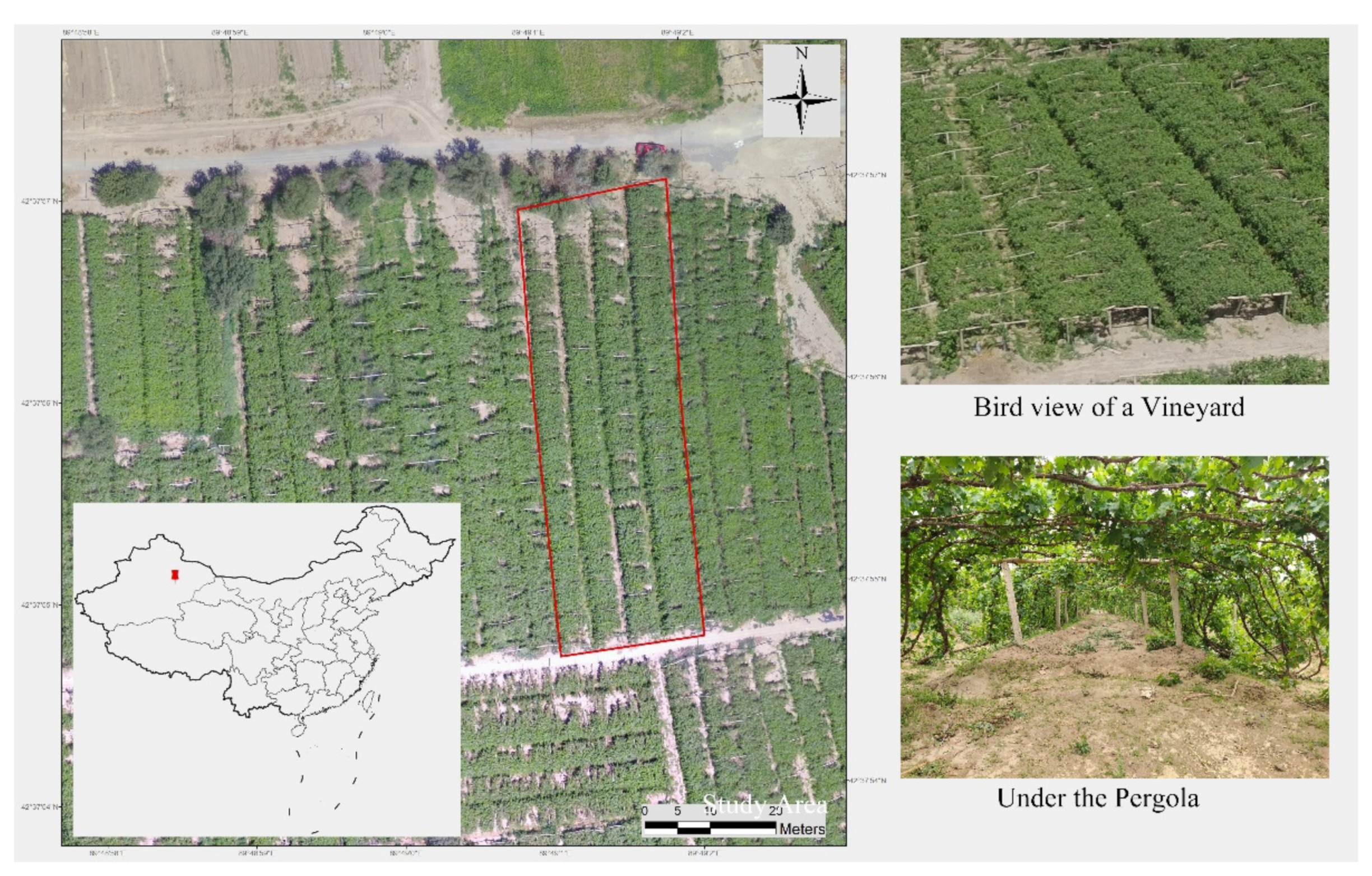
The study was carried out in Turpan city, Xinjiang, one of the largest table grape growing regions in China, where significant interests are arising in the development of strategies to ensure grape quality and yields [63] in recent years. Turpan has a continental warm temperate desert climate with a mean annual precipitation of 16.4 mm and a mean annual temperature of 13.9 °C (1950–2011). Extreme temperatures reach 47.8 °C (2008) in summer and −28.0 °C (1960) in winter [64,65]. In general, vine plants are buried under the soil during winter to protect them from freezing, and then unearthed in spring. The most widespread vine type in Turpan is Vitis vinifera L. cv. Thompson seedless, which has a good reputation for high sugar content and good quality and, therefore, is a suitable research subject for this study.
The experiment was conducted from May to August 2021 in a small vineyard in Pichan County (Figure 1). The vines were 10 years old, planted in five ditches, where two of them were attached on one pergola from two sides, and the other three were attached on separate pergolas. The planting spaces between vines were approximately 1.50 m, and the distances between ditches were approximately 6.00 m with an average pergola height of 1.60 m. The vines were unearthed and first irrigated on 16 and 26 March 2021.
2.2. Data
2.2.1. Unmanned Aerial Vehicle (UAV) Data Acquisition
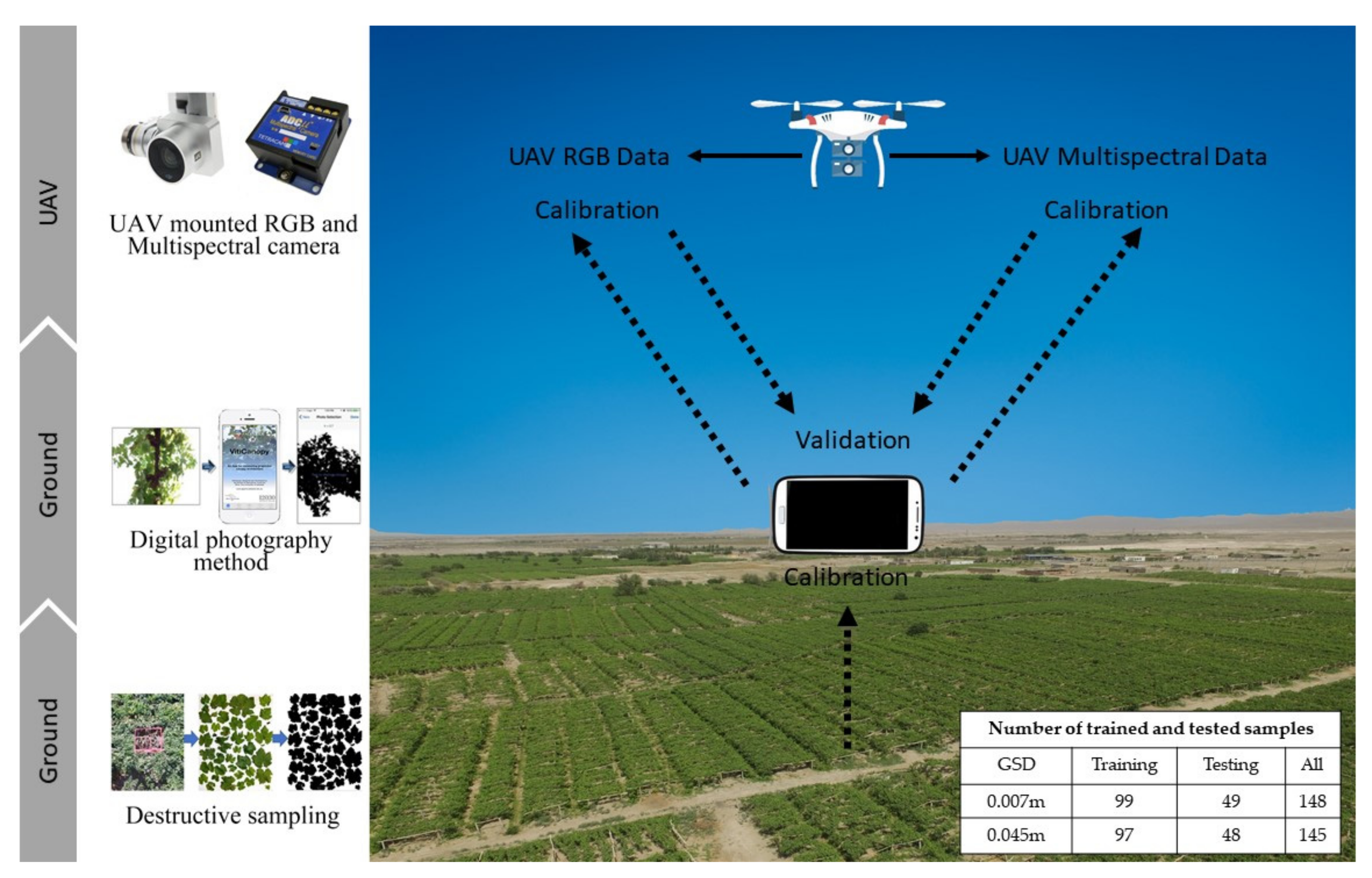
Data were collected from May to August 2021, covering the main important growing seasons. Drone-based RGB and multispectral images were captured from flight heights of 17 m and 91–100 m to generate images of 0.007–0.008 m and 0.040–0.045 m with spatial resolutions (or ground sample distance (GSD)). Two flight heights were used because the lower flight height data can be used for smaller vineyards with higher spatial resolutions, and higher flight heights can be used to monitor larger fields. An overlap of 80–90% at the front and 60–80% at the side was maintained. This overlap ensured creation of good quality orthomosaic images. The UAV (DJI Phantom 3 Advanced, SZ DJI Technology Co., Ltd., Shenzhen, China) has characteristics of stable flight, and has a flight time of about 15 min/battery. It is equipped with a remote controller, a global navigation satellite system (GNSS) receiver, and autonomous flights were carried out using the Pix4Dcapture app (Pix4D SA, Lausanne, Switzerland) on an Android smartphone.
RGB images were captured using the built-in camera of the UAV. It was attached to a three-axis gimbal mount to provide stability, it has a 12.4-megapixel sensor, which allows the acquisition of RGB images with a maximum image dimension of 4000 × 3000 pixels. A multispectral camera of Tetracam ADC Micro (Tetracam, Inc., Gainesville, FL, USA) was installed on the UAV, with an image dimension of 1280 × 1024 pixels. The ADC Micro is a single-sensor digital camera designed and optimized for capturing visible light wavelengths longer than 520 nm and near-infrared wavelengths up to 920 nm, with three fixed green, red, NIR filters (equivalent to Landsat TM2, TM3, TM4) [66]. The primary design of this product is to record vegetation canopy reflectance [67,68], and multi-spectral earth-observing satellites such as Landsat ETM, SPOT, and IKONOS obtain spectral information in the same few broad wavebands [69]. The multispectral images were taken simultaneously with RGB images in RAW format, then calibrated and converted to TIF format using PixelWrench2 software.
The RGB and multispectral images were then mosaiced using the photogrammetric software Pix4DMapper (Pix4D SA, Lausanne, Switzerland). Ground control points (GCPs) were distributed evenly in the study area, and coordinates were measured using real-time kinematics (iRTK2, Hi-Target Satellite Navigation Technology Co., Ltd., Guangzhou, China) with an error range of ±10 mm. The schedules of the missions are listed in Table 1. The final images were resampled to 0.007 m and 0.045 m spatial resolutions for 17 m and 91–100 m flight heights, respectively, after preprocessing. For convenience, we abbreviated the different spatial resolution and sensor data as follows: the data derived from 0.007 m spatial resolution of the multispectral sensor are called the 0.007 m GSD MS dataset; the data derived from 0.007 m spatial resolution of the RGB sensor are called the 0.007 m GSD RGB dataset; the data derived from 0.045 m spatial resolution of the multispectral sensor are called the 0.045 m GSD MS dataset; and the data derived from 0.045 m spatial resolution of the RGB sensor are called the 0.007 m GSD RGB dataset.
2.2.2. Leaf Area Index (LAI) Data Acquisition by Destructive Sampling
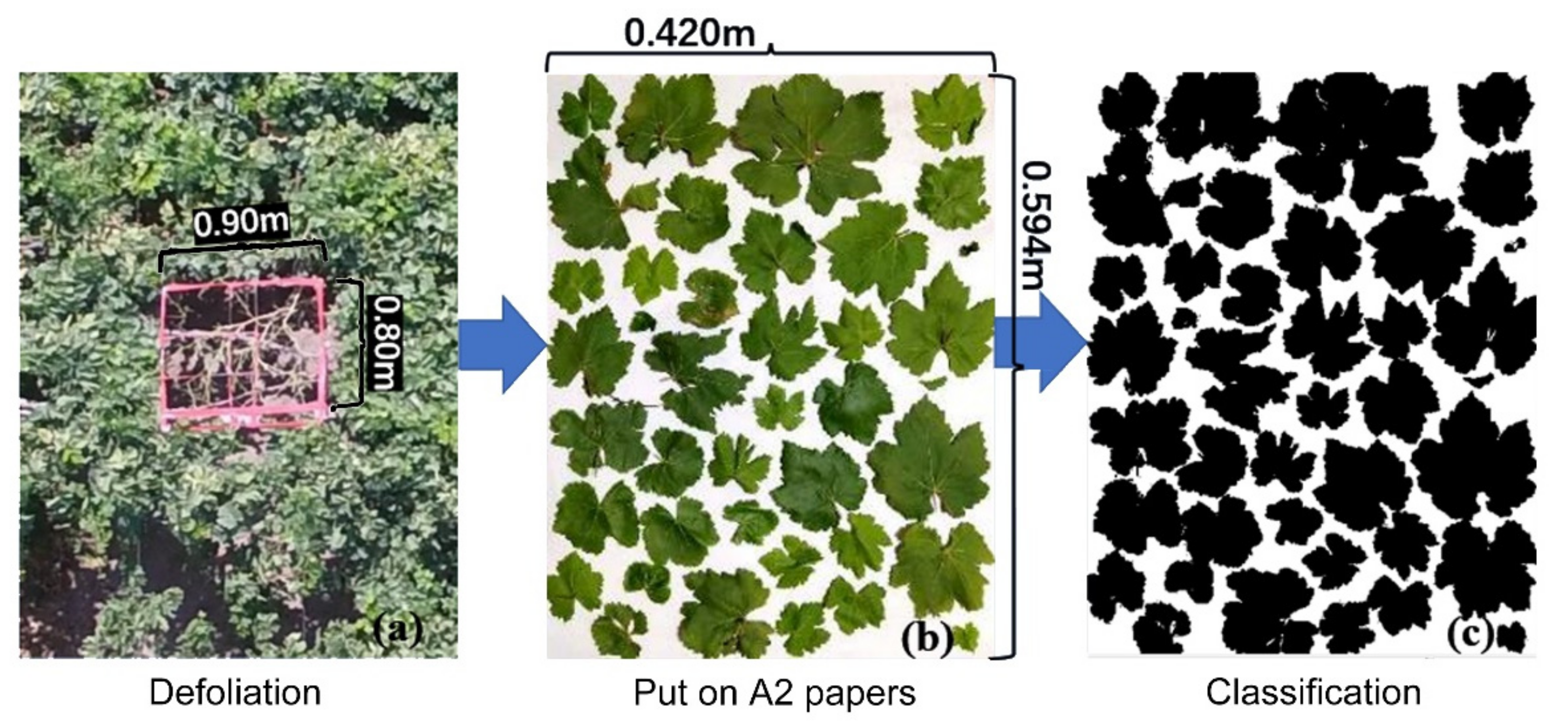
To calibrate the VitiCanopy parameters, the true LAI values were obtained using a destructive sampling method (Figure 2). The experiment was carried out from 7–9 August 2021. Ten samples of the vineyard LAI were measured using a 0.80 m × 0.90 m rectangular iron frame to separate the samples of vine leaves measured by VitiCanopy. Sampling points were selected after detailed inspection of the field survey on the sampling day to cover characteristic LAI values, of which the thickest and sparsest areas were both taken into consideration. We added an extra plot that did not include any canopy for representing the zero value of the LAI. The spatial distribution of the samples is shown in Figure 3. The procedure was as follows [5]: (1) carry out the UAV mission and VitiCanopy measurements in the same day; (2) install a rectangular wire frame at each plot with a size of 0.80 m × 0.90 m which corresponds to VitiCanopy measurements, and collect all leaves inside the frame; (3) put the leaves on white A2 paper (0.594 m × 0.420 m) and photograph with a digital RGB camera; (4) classify the pictures as leaf and non-leaf areas using ENVI5.3 (Harris Geospatial Solutions, Broomfield, CO, USA), and calculate the leaf area of each sample. The Greenness Index was used to distinguish leaf area in this study [70]. The LAI was then calculated by dividing the accumulated leaf area of the samples at each site into the area of the rectangular wire frame. The locations of the destructive samplings were confirmed by comparing the orthoimages before and after defoliation.
2.2.3. LAI Data Acquisition by Digital Cover Photography Method
LAI values were measured using a free smartphone and tablet PC application called VitiCanopy, which was developed to measure the LAI of vineyards, and proved to be effective for vertical shoot positioning (VSP) trained vineyards with a light extinction coefficient of 0.70 [21,71]. It was also proved that this application was valid for other tree crops such as cherry [72], cocoa [73] and apple trees [22] by adjusting input parameters such as the light extinction coefficient.
The measurements were carried out near the girders for convenience of marking, so the positions could be easily located in orthomosaic UAV images for later calculations, as shown in Figure 3. The pictures were taken approximately 0.80 m below the pergola, as suggested by the software developer [21], and cover about 0.80 m × 0.90 m of the rectangular region. Applying the default light extinction coefficient of 0.70, approximately 40–60 plots were measured in four different growing stages, including non-leaf area and very dense vegetated regions. Low-quality measurements were removed based on the picture quality as assessed by VitiCanopy. The number of samples used in different sensor and GSD datasets were given in Table 2. The software performs a cloud-filtering process and automatic gap analysis of upward-looking digital images [74]. The light extinction coefficient was then optimized using the true LAI values, which will be discussed in the following sections.
2.3. Methods
The overall workflow of this study consists of three key steps: (1) calibration of the light extinction coefficient by the digital cover photography method using a destructive sampling method; (2) calculation of VIs from UAV-based multispectral and RGB images; and (3) calibration and validation of VI-LAI models using LAI values from the first step and VIs from the second step (Figure 4). This study adopted the World Geodetic System 1984 (WGS1984) as the coordinate system for georeferenced images, maps, or any others in this paper, if not particularly indicated.
2.3.1. Determination of Light Extinction Coefficient
The digital cover photography method can estimate the LAI values of many vegetation types [22,72]. The VitiCanopy application was developed on the basis of the digital cover photography method [21], which obtains the number of total pixels, big gaps, and total gaps of vegetation area from pictures, and then calculates the fractions of foliage cover and crown cover by applying the following equations [17]:
where the is the foliage cover, is the crown cover, is the total number of gap pixels, is the total number of pixels, and is the total number of big gap pixels. Using the calculated and values, the crown porosity, clumping index at the zenith, and the effective leaf area index can be calculated from Beer’s Law [74,75]:
where is the crown porosity, is the clumping index, is the effective leaf area index, and k is the light extinction coefficient, which was set at 0.70 as the default. Therefore, the light extinction coefficient can be calculated by inverting Equation (5) and using the measured true LAI values () as follows [22]:
We can take the average of k values, as in many other studies [26,29]. We also experimented with a variable k for better estimation of the LAI by investigating the correlations with other parameters, such as the fraction of foliage cover (), as studied by Poblete et al. (2015) [22]. The optimized k values were used to calculate the LAI values of other sampling points, which were used as ground truth data for LAI estimation models, as stated in the following steps.
2.3.2. Spectral Feature Extraction and Reduction
Modeling using only three band spectral data is a time-saving method, but its accuracy is difficult to guarantee. Therefore, based on the Index Database website (https://www.indexdatabase.de/, last accessed on 30 September 2021), 32 vegetation indices (VIs) were calculated using one to three spectral bands from each sensor, where 17 VIs are from multispectral data and 19 VIs are from RGB data (Table 3). Among these, R, G, GtoR, and RmG can be applied to both sensors. For every rectangular area that VitiCanopy could detect (Figure 3), the average VI values were calculated. These VI values were used as variables for the LAI estimation models, which will be introduced in the following sections. Calculations were performed using the GDAL library in Python.
In supervised learning, the models based on all variables (VIs) may show better performance than using only three band data but require higher computing capacity. To overcome the calculation expenses and improve the accuracy, we implemented feature (the VI in this study) selection procedures, which maintain useful information with highly correlated VIs and exclude redundant ones from regression analysis [91]. Feature selection methods are of great importance in the field of data mining [92] and help to obtain good or better accuracies in predictive models while requiring less data. Using fewer attributes is desirable because it reduces the complexity of the model, and a simpler model is simpler to understand and explain [93]. Therefore, the selection of variables is an important step in improving the efficiency of models.
In this study, we carried out feature selection using the recursive feature elimination (RFE) approach, which is a widely applied method and performed well in previous studies [94,95,96]. It was performed in two steps: (1) running an estimator to determine the feature importance, and (2) removing the feature with the lowest importance score and evaluating the model performance. The built-in feature selection method of random forest (RF) was used in this study to derive the importance of each variable in the tree decision [97]. We implemented the process 300 times to obtain the feature importance in step (1), and determined the features to participate in the final modeling in step (2).
2.3.3. Ensemble Model Development
To enhance the prediction performance, an ensemble model was proposed based on the voting strategy, including the following steps: (1) training and applying multiple machine learning models independently and (2) combining multiple prediction results through voting [98]. In this study, the voting regressor was used; it is a composite strategy across ML models and performed best on average across subjects. Five ML regression methods were employed as the base learners to construct the ensemble learning, namely, the SVR, RFR, PLSR, GBR, and KNN. These are widely used in many studies [95,96,99,100]. The entire dataset was randomly split into training and testing sets to implement the independent validation. One-third of the whole dataset was used for validation (three-fold), which was determined by comparing the results 2–10 fold, while two-thirds were used for training. For the RFR method, the number of trees was 600, the minimum sample leaf was set to 3, and the maximum depth was 10. For the SVR method, the “linear” was used as the kernel, because it has the best performance among all the tests. In the GBR method, the number of boosting stages was set to 30. Six was set for the number of estimators in the PLSR methods, while three was set for datasets with only three variables. Three was chosen as the number of nearest neighbors for the KNN method. All parameters were chosen using the tuning and grid search methods.
The modeling tests were carried out using datasets of 0.007 m and 0.045 m GSD data separately. To test the robustness of all the models, 100 repetitions of three-fold cross validation were performed, resulting in a total of 300 experiments. To assess the performance of these models, the coefficient of determination (R2), root mean squared error (RMSE), and mean absolute error (MAE) were calculated as follows:
where is the measured value, is the predicted value, is the average of the measured values, and n is the number of samples. Modeling and accuracy assessments were implemented using the scikit-learn packages in Python.
3. Results
3.1. Calibration Result of Light Extinction Coefficient
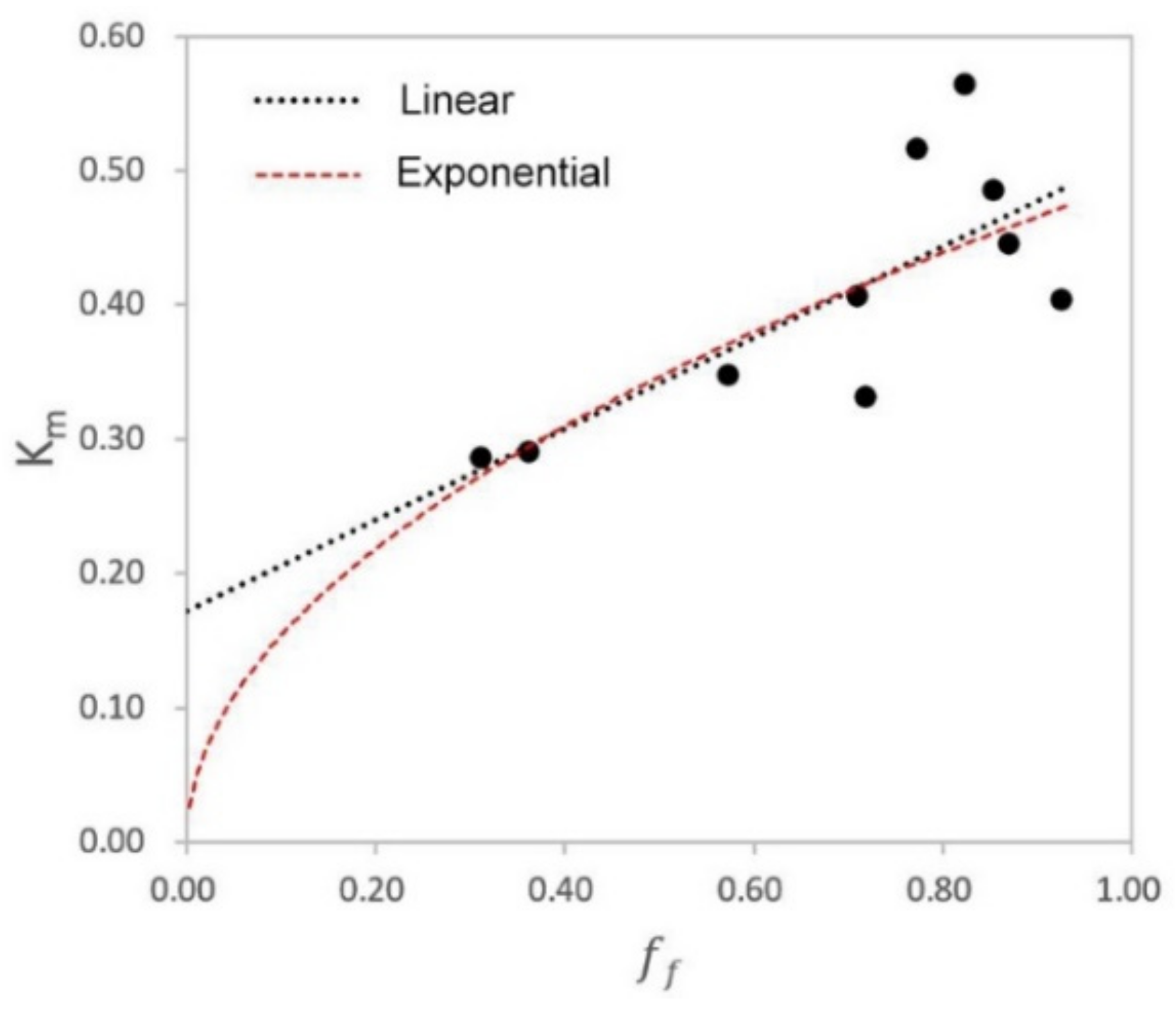
We attempted to find a variable k, which ranged from 0.29 to 0.56, for better estimation of LAI, and we found that they have certain correlations with the fraction of foliage cover () (Table 4), which is in line with a previous study of Poblete et al. (2015) [22]. Although R2 was larger in the exponential model, according to the RMSE, the linear model showed higher performance than the exponential model. However, considering that we have only 10 samples of leaf area (we did not include the k value for the non-leaf plot, since it cannot be calculated because the denominator was zero in Formula (6)), and its linearity was not obvious with an R2 of 0.57 only (Figure 5), we chose to use the average k value (0.41) and apply it to the LAI calculations as stated in the previous studies.
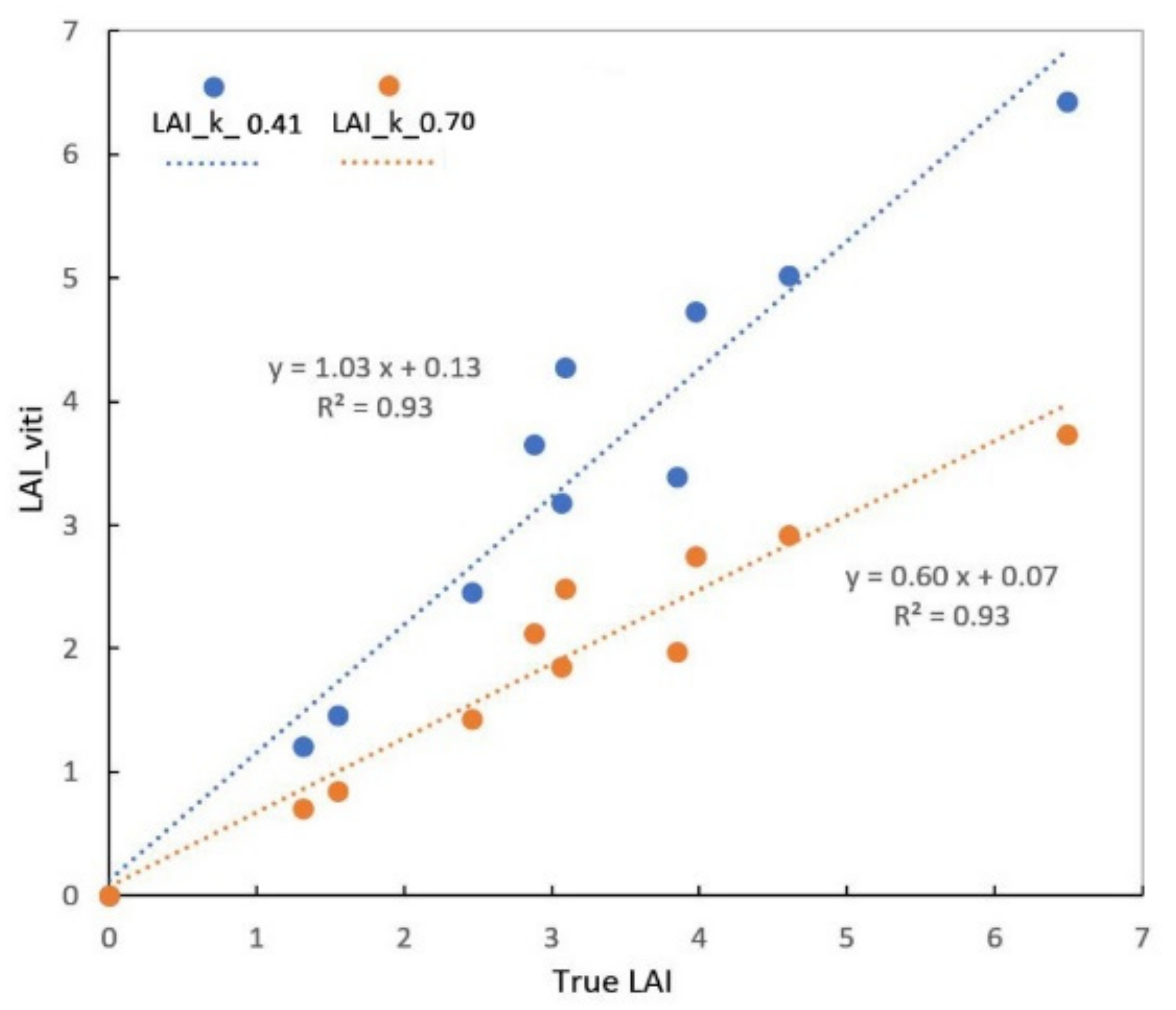
The correlations between the true LAI and the values based on VitiCanopy, using the default and optimized k values, are shown in Figure 6. As seen, the LAI values from VitiCanopy after optimizing k were closer to the true values with a slope of 1.03, indicating that a k value of 0.41 would be suitable for pergola-trained vineyards. For decreasing the accumulated error between the true LAI and the LAI from VitiCanopy (k = 0.41), LAI_k_0.41 were corrected again using the relationship shown in Figure 6.
3.2. Vegetation Indices and Selection
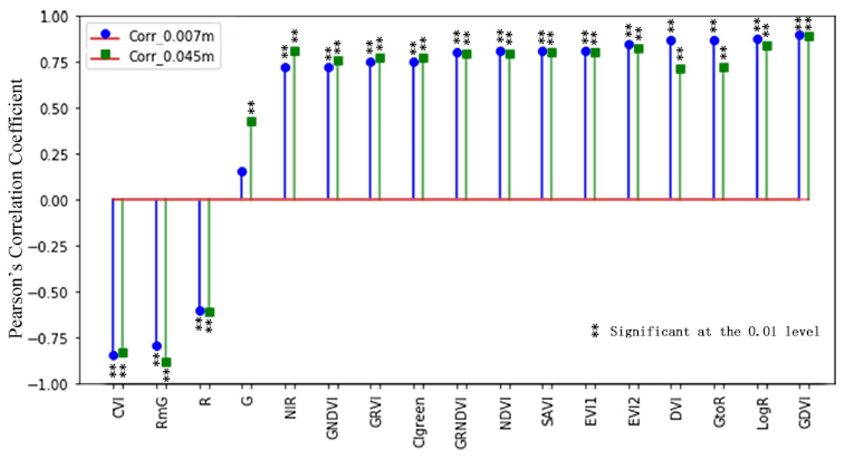
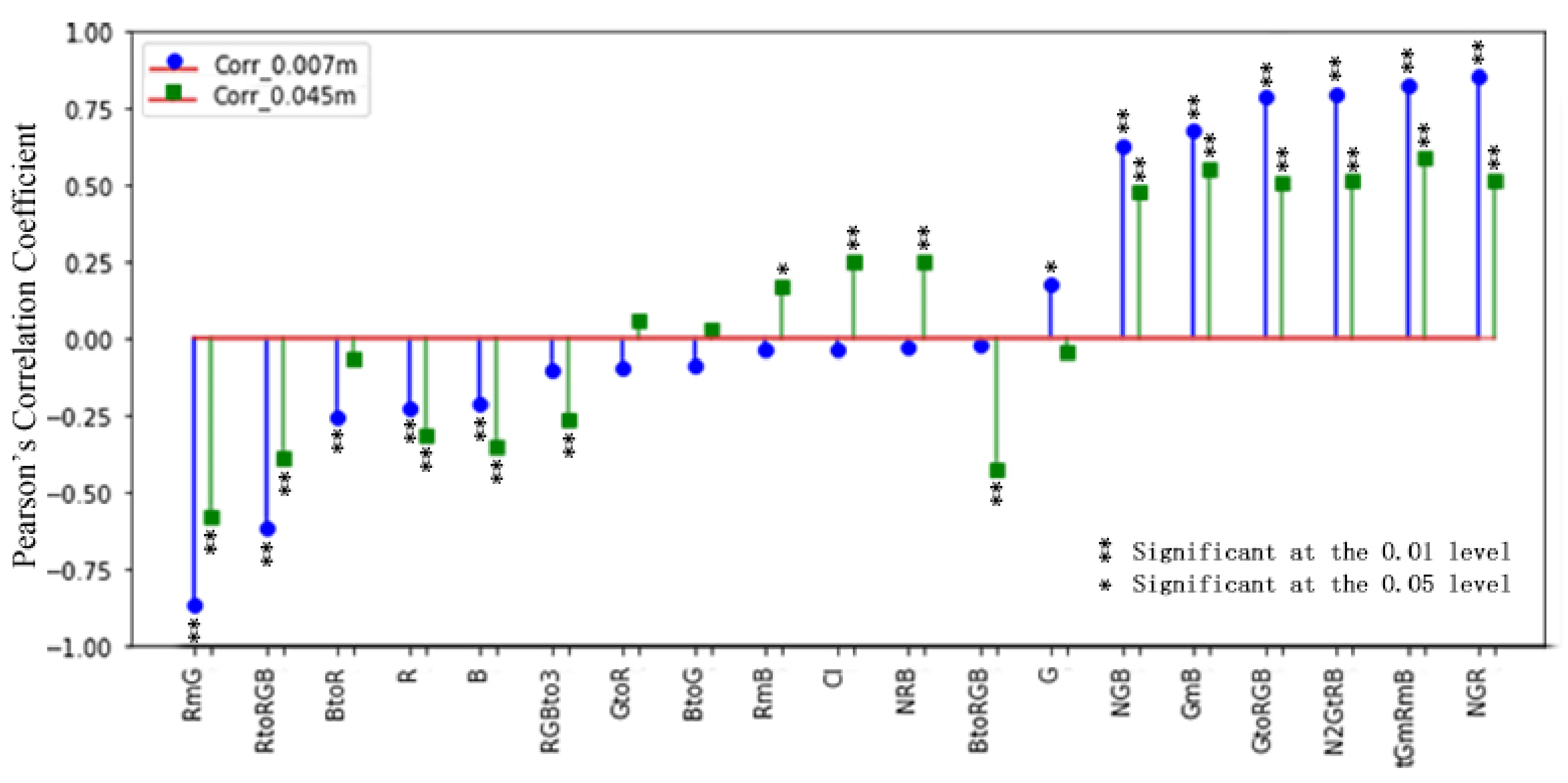
The optimized LAI values, which were based on VitiCanopy measurements, and VIs from both UAV RGB and multispectral data were compared. As seen in Figure 7, all 17 VIs from multispectral data showed strong correlations with the LAI, except for the green band. GDVI showed the best correlation with a Pearson’s correlation coefficient of 0.903 significant at the 0.01 level, while the green band showed the lowest correlation. Among the 19 VIs from RGB images, only eight showed better correlations (Figure 8), and 0.007 m and 0.045 m GSD data showed large discrepancies in the same VIs.
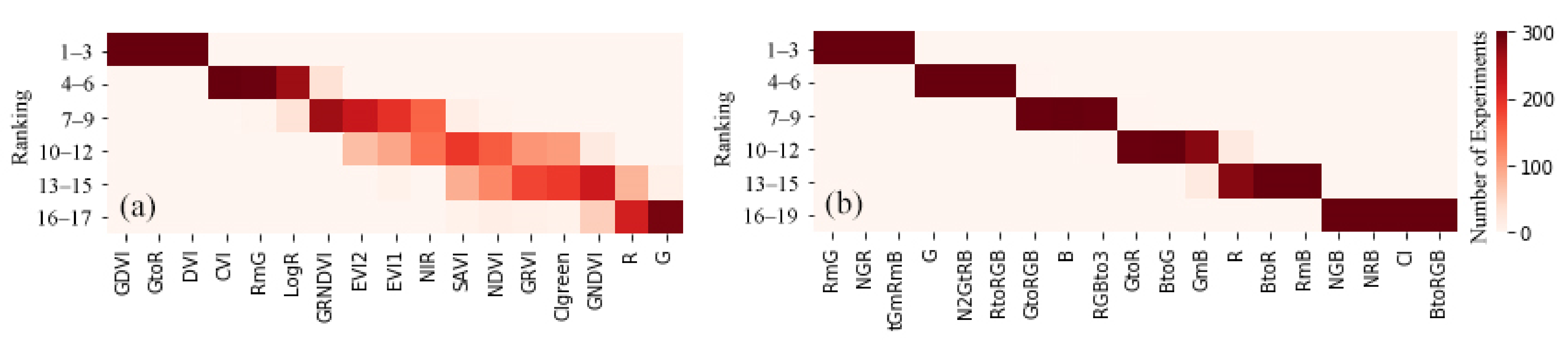
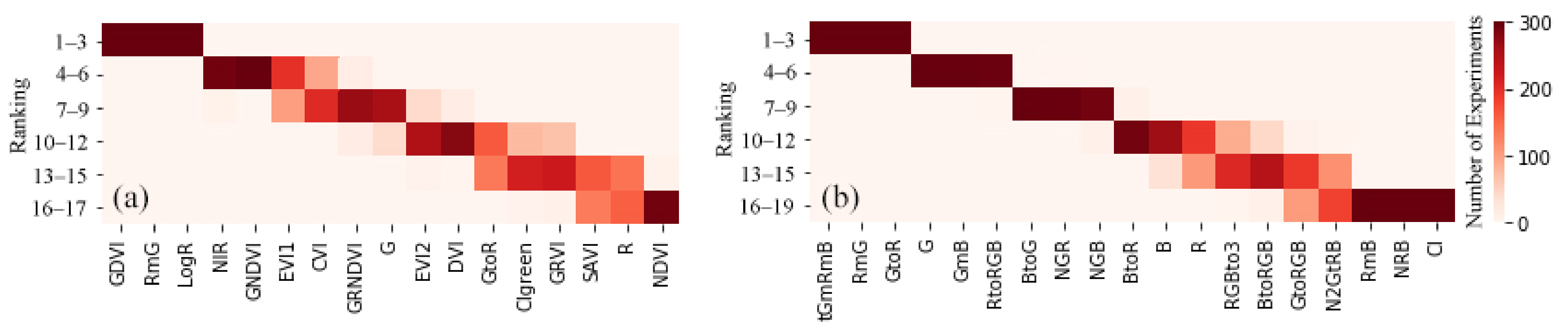
The 17 VIs from the multispectral sensor and 19 VIs from the RGB sensor at different spatial resolutions were ranked using the RFE strategy described in Section 2.3.2. Figure 9 shows the VI rankings for 0.007 m GSD data, and Figure 10 shows the rankings of VIs for 0.045 m GSD data. Most of the VIs have stable ranking orders, where the rankings were obtained from 300 repeated experiments. For example, GDVI, GtoR, DVI, CVI, and RmG are mostly highly ranked in 0.007 m GSD data from multispectral sensors, and almost all VIs ranked stably in 0.007 m GSD data from the RGB sensor.
3.3. Model Comparison and Performance
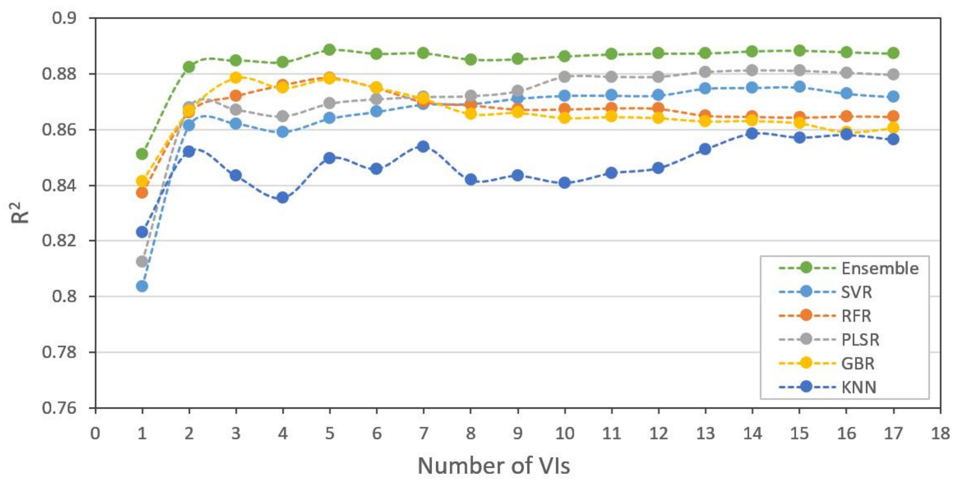
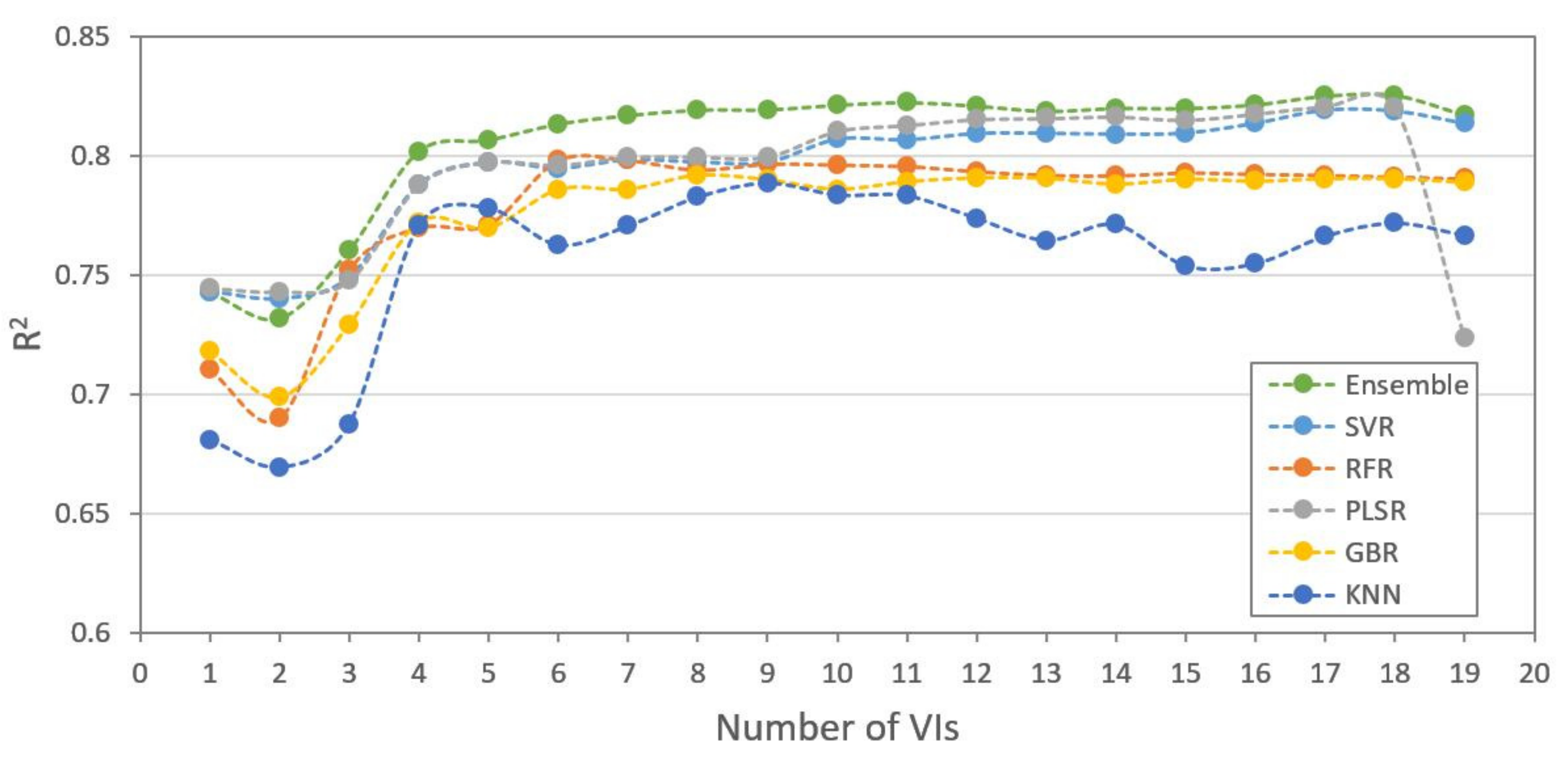
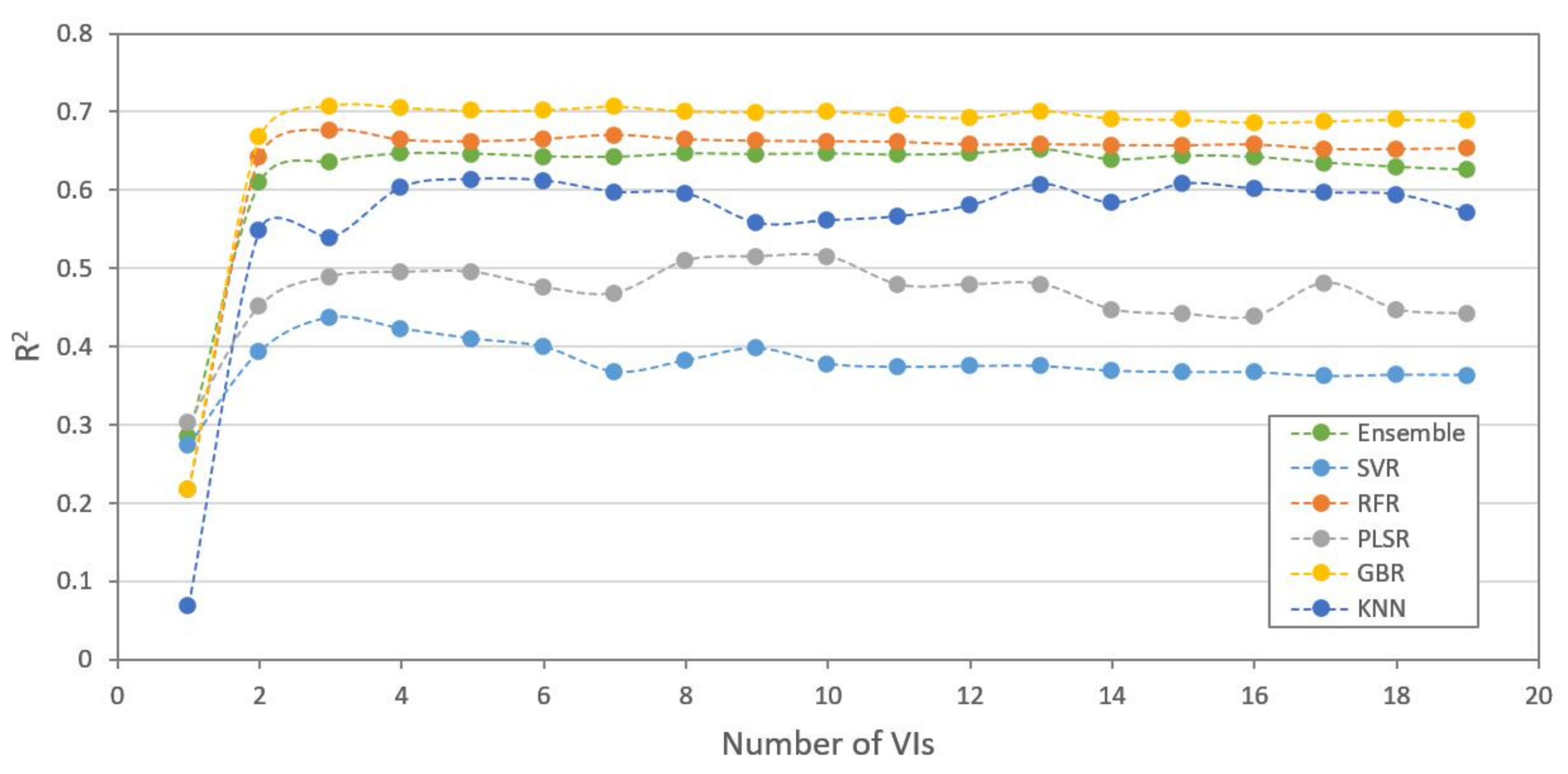
According to the rankings of VIs for four different datasets (0.007 m GSD MS, 0.007 m GSD RGB, 0.045 m GSD MS, 0.045 m GSD RGB), we iteratively added the top ranked VIs one by one into the ML models and updated the model performance until all VIs were included. Every experiment was conducted 100 times with three-fold cross validation, and the training accuracies obtained by the five base models and ensemble model were calculated. The results of the 0.007 m GSD MS dataset are shown in Figure 11. As shown, RFR and GBR achieved the highest performance when five VIs were included among the five base models. The others achieved the best performance when 14 VIs were included. The accuracy of the ensemble model reached the highest while including five VIs. The results for the other datasets are given in the Appendix A (Figure A1, Figure A2 and Figure A3). In the same way, we chose 10 VIs for the 0.045 m GSD MS dataset, 18 VIs for the 0.007 m GSD RGB dataset, and three VIs for the 0.045 m GSD RGB dataset.
In addition, we trained all base models and ensemble models in full and selected features, as well as using only the three-band data on training samples, and evaluated the model performance on test samples. The test accuracies of 300 experiments (100 times of three-fold cross validation) for the 0.007 m GSD MS dataset are shown in Table 5. Satisfactory accuracies were achieved by all approaches, demonstrating the effectiveness of these models in LAI estimation in pergola-trained vineyards. In particular, the ensemble model outperformed all the base models, achieving an R2 of 0.830 using the three-band data, 0.887 using all VIs, and 0.889 using the selected five VIs. The test accuracies of other datasets with different variables are provided in the Appendix A (Table A1, Table A2 and Table A3).
3.4. Model Adaptability for Different Datasets
Then, we evaluated the model adaptability under different GSD and sensor datasets. Table 6 shows the R2, RMSE, and MAE of all the base models and ensemble models using the different datasets. Generally, all models achieved good results except for the 0.045 m GSD RGB dataset, where SVR showed the lowest performance. Among the base models using 0.007 m GSD data, RFR and GBR performed better than others in the MS dataset, whereas SVR and PLSR outperformed others in the RGB dataset; for the base models using 0.045 m GSD data, SVR and PLSR showed better performances than others in the MS dataset, and RFR and GBR performed better than others in the RGB dataset. The ensemble model outperformed all the base models in most cases.
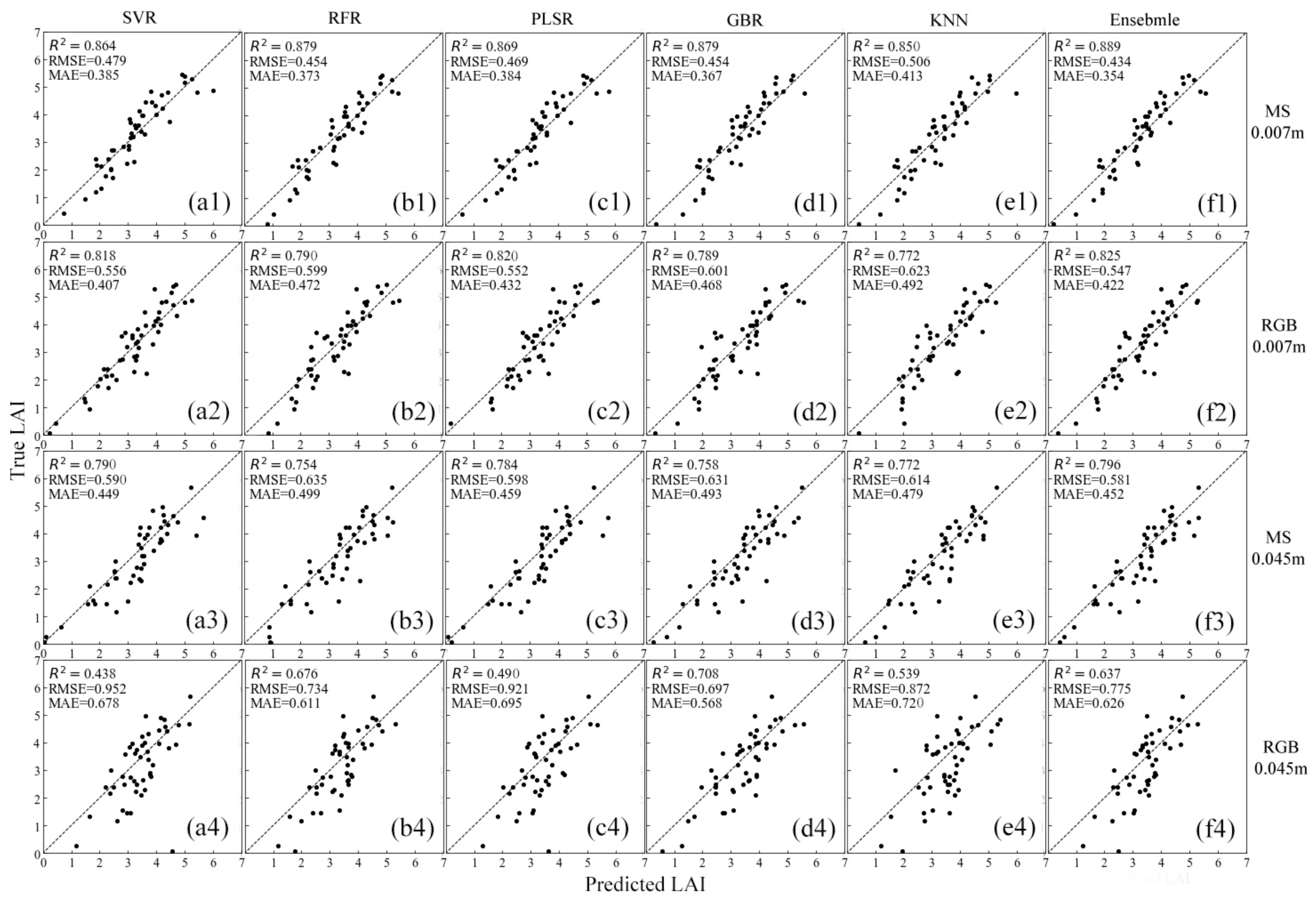
The agreement between the true LAI (optimized from the VitiCanopy results) and the predicted LAI of each model using the selected features for each dataset is shown in Figure 12. Among all models, the best agreement was found in the ensemble model using the 0.007 m GSD MS, 0.007 m GSD RGB, and 0.045 m GSD MS datasets (Figure 12(f1–f3)).
4. Discussion
4.1. Contributions of Feature Selection for Datasets
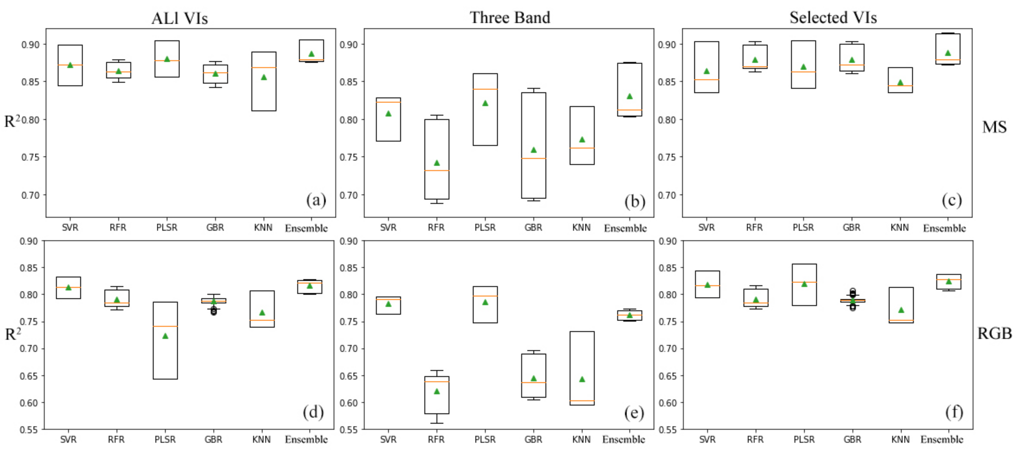
This study explored the potential of UAV data as an alternative method for LAI extraction for pergola-trained vineyards. Many vegetation growth variables can be accurately and remotely retrieved from satellite and UAV-based remote-sensing data for different vegetation types, and they have been used to carry out precise management [101]. In their study on the ratio indices of rice (e.g., CIgreen) using UAV data (the same series of multispectral sensors as in our study), Yang et al. (2021) showed the lowest correlation with LAI, and EVI2 had a relatively higher correlation, while the normalized indices (NDVI) had the median [102]. In their study on selection of vegetation indices for mapping the sugarcane condition, Susantoro et al. (2018) showed the DVI and GNDVI derived from Landsat8 were highly correlated to LAI [103], which is in agreement with our study. ML methodologies can be used to effectively analyze and utilize information-rich datasets as well as high-dimensional observation data. However, the performance of different ML methods varies with different datasets. For the data obtained by hyperspectral sensors, machine learning methods can be used to directly choose the best related spectral bands to train the models [47,104]. It is possible to obtain better performance by calculating vegetation indices and using them as independent variables [96]. Compared to hyperspectral sensors, relatively fewer spectral data can be obtained from multispectral sensors. In our study, modeling using only three-band spectral data saves time, while also making it possible to obtain good results. For example, the R2 for the ensemble model, which was based on 0.007 m GSD MS data, reached 0.830 (Table 5). However, this is not always the case, especially for sensors such as those on the RGB camera. In this case, none of the three bands were highly correlated to LAI (Figure 8), and most of the models had low accuracies. Figure 13 and Figure 14 show the performances of different models in different datasets with different combinations of variables. The models based on all variables (VIs) showed better performance than those using only three band data, for both multispectral and RGB data. However, they required more computing capacity. The models based on only three-band data showed lower stability than those based on all variables. In brief, feature selection improved model performance compared to that when using all features (VIs) or only three band data. This was observed in both multispectral and RGB data.
4.2. Comparing Different Machine Learning Methods in Different Datasets
In addition to the selection of vegetation indices, the regression algorithm itself is another crucial factor that affects LAI estimation accuracy. A suitable model can help improve the accuracy of LAI predictions from remote-sensing data. Figure 13 and Figure 14 also show the performances of the different models in different datasets.
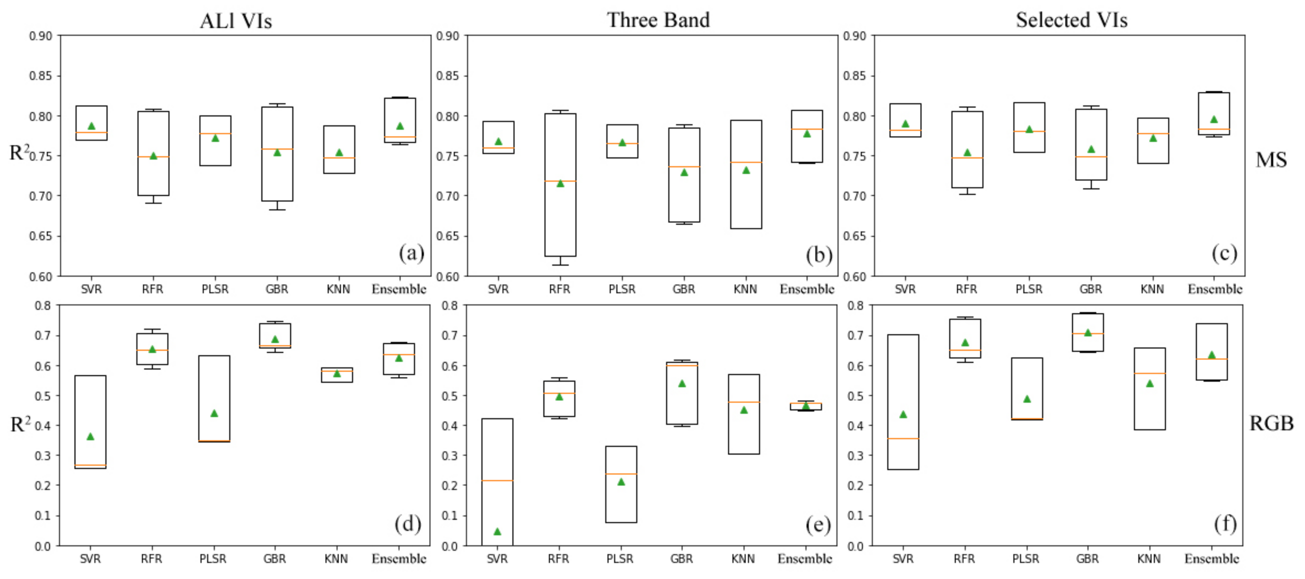
All base models used in this study have been commonly applied in many studies, and all models have their advantages in specific situations. SVR and PLSR perform better in higher dimensional datasets, as reported in previous studies [51], but they show lower accuracy and stability with possibly noisy datasets (Figure 14f). The RFR method, which is less likely to overfit [54], showed higher stability in all datasets. SVR outperforms RF in most cases in MS data, and this result is in line with a previous study by Grabska et al. (2020) when using Sentinel-2 imagery [105]. The GBR method showed a higher stability in most cases. All base models showed satisfactory accuracies except for the 0.045 m GSD RGB data, where the SVR performed the worst, with an R2 of 0.438.
However, instead of using a single machine learning model, we developed an ensemble model that combines five base learners. Our results show that the ensemble model outperformed all base models (again, except for the 0.045 m GSD RGB dataset) significantly both using all variables or selected ones, as well as using only the three-band data. With selected VIs, the ensemble models obtained 0.889 in R2, 0.434 in RMSE, and 0.354 in MAE, and achieved an increase of 1.14%, 4.41%, and 5.09%, respectively, compared to the best single base model in the 0.007 m GSD MS dataset. For other datasets, the ensemble models achieved 0.825, 0.796, and 0.637 in R2 for 0.007 GSD RGB, 0.045 m GSD MS, and 0.045 m GSD RGB datasets, respectively.
4.3. Effects of Different Ground Sample Distance (GSD) and Sensor Datasets
Accurate positions of proximal measurements were difficult to locate in lower spatial resolution data, which also contained more mixed pixels. This may be one reason the models based on the 0.045 m GSD datasets showed lower performances than those based on the 0.007 m GSD datasets. The models based on multispectral data showed better performance compared to those based on RGB data, as vegetation types can be easily differentiated by near-infrared and red regions [32,106] and RGB images only distinguish the green canopies according to their surface colors. In addition, all single bands of the RGB sensor were weakly correlated to the LAI (Figure 8), which may be another reason the datasets from the RGB sensor showed a lower performance than those from the multispectral sensor. The performance of different ML methods varies according to datasets: multispectral sensors would be the best choice for LAI estimations, but RGB sensors can also be used as a low cost and easily available alternative.
5. Conclusions
By integrating remote-sensing data with machine learning techniques, our study demonstrated the potential of UAV-based remote-sensing data in the estimation of LAI variations in pergola-trained vineyards. It provides a solid ground for further applications, such as precision viticulture.
In summary, this study achieved the following results:
- (a)
- We proposed a light extinction coefficient that is suitable for estimating the LAI in pergola-trained vineyards. The LAI values estimated using the proposed light extinction coefficient of 0.41 were closer to the true LAI, using which in situ LAI values can be estimated quickly by the use of portable devices such as mobile phones or tablets.
- (b)
- We propose a robust VI-LAI estimation ensemble model that outperforms other base models. Among these, those using multispectral data-derived VIs showed higher potentiality than RGB data-derived ones. However, RGB data were also found to be a promising data source with an R2 reaching 0.825, RMSE 0.546, and MAE 0.421.
- (c)
- Feature selection improved the accuracy and efficiency of LAI estimation models by using the best combinations of VIs from both multispectral and RGB data.
This study is the first to apply UAV remote-sensing data to assess the LAI of pergola-trained vineyards. Compared to manual ground measurements, it has the advantages of high efficiency, time saving, and suitability for obtaining LAIs in large vineyards. However, it also had some limitations because we used different spatial resolution data at different crop stages as the whole dataset and assumed that the VI-LAI relationship does not change over the whole season. Therefore, we see our study as an initial step for developing a larger-scale and real-time LAI estimation method for pergola-trained vineyards, and we recommend using multiple data sources such as hyperspectral, LiDAR, and thermal sensors to obtain more information. We also recommend developing better LAI estimation models in different spatio-temporal conditions. More advanced instruments and methods, such as deep learning, as well as more specific datasets, will improve the accuracy of estimation models.
Author Contributions
Conceptualization, O.I. and A.K.; methodology, Q.D.; software, O.I.; validation, O.I. and A.K.; formal analysis, O.I.; investigation, O.I.; resources, A.K.; data curation, O.I.; writing—original draft preparation, O.I.; writing—review and editing, A.K.; visualization, O.I.; supervision, Q.D. and A.K.; project administration, Q.D.; funding acquisition, Q.D. All authors have read and agreed to the published version of the manuscript.
Funding
This research was funded by The National Key Research and Development Programme of China, Grant/Award Number: 2016YFC0803106.
Institutional Review Board Statement
Not applicable.
Informed Consent Statement
Not applicable.
Data Availability Statement
The data are not publicly available due to the continuing related research.
Acknowledgments
The authors would like to thank Abliz Ilniyaz, Erkinjan Abliz, Sulayman Abdul, Dawut Hoshur, Ghoji Mengnik and others for their help in field work.
Conflicts of Interest
The authors declare no conflict of interest.
Appendix A

Table A1.
Test accuracies including mean and standard deviation of five base models and an ensemble model trained on the 0.007 m GSD RGB dataset in different number of VIs.
Table A1.
Test accuracies including mean and standard deviation of five base models and an ensemble model trained on the 0.007 m GSD RGB dataset in different number of VIs.
| ML Methods | Using All 19 VIs | Using Selected 18 VIs | Using 3 Bands | ||||||
|---|---|---|---|---|---|---|---|---|---|
| R2 | RMSE | MAE | R2 | RMSE | MAE | R2 | RMSE | MAE | |
| SVR | 0.813 (0.016) | 0.565 (0.021) | 0.415 (0.020) | 0.818 (0.021) | 0.556 (0.028) | 0.407 (0.023) | 0.783 (0.014) | 0.608 (0.008) | 0.453 (0.011) |
| RFR | 0.790 (0.015) | 0.599 (0.029) | 0.471 (0.011) | 0.791 (0.015) | 0.598 (0.028) | 0.470 (0.010) | 0.623 (0.033) | 0.804 (0.052) | 0.610 (0.018) |
| PLSR | 0.723 (0.059) | 0.684 (0.069) | 0.485 (0.041) | 0.820 (0.032) | 0.552 (0.037) | 0.432 (0.045) | 0.787 (0.029) | 0.602 (0.027) | 0.447 (0.023) |
| GBR | 0.787 (0.007) | 0.604 (0.015) | 0.471 (0.014) | 0.790 (0.005) | 0.600 (0.015) | 0.467 (0.007) | 0.645 (0.034) | 0.779 (0.055) | 0.600 (0.023) |
| KNN | 0.766 (0.029) | 0.630 (0.028) | 0.496 (0.020) | 0.772 (0.030) | 0.623 (0.030) | 0.492 (0.023) | 0.643 (0.063) | 0.777 (0.058) | 0.602 (0.046) |
| Ensemble | 0.817 (0.011) | 0.560 (0.006) | 0.432 (0.016) | 0.825 (0.012) | 0.546 (0.007) | 0.421 (0.019) | 0.762 (0.008) | 0.638 (0.012) | 0.489 (0.020) |
Table A2.
Test accuracies including mean and standard deviation of five base models and an ensemble model trained on the 0.045 m GSD MS dataset in a different number of VIs.
Table A2.
Test accuracies including mean and standard deviation of five base models and an ensemble model trained on the 0.045 m GSD MS dataset in a different number of VIs.
| ML Methods | Using All 17 VIs | Using Selected 10 VIs | Using 3 Bands | ||||||
|---|---|---|---|---|---|---|---|---|---|
| R2 | RMSE | MAE | R2 | RMSE | MAE | R2 | RMSE | MAE | |
| SVR | 0.787 (0.019) | 0.594 (0.018) | 0.451 (0.027) | 0.790 (0.018) | 0.590 (0.017) | 0.449 (0.024) | 0.768 (0.017) | 0.620 (0.030) | 0.475 (0.003) |
| RFR | 0.751 (0.044) | 0.638 (0.036) | 0.500 (0.028) | 0.754 (0.041) | 0.635 (0.032) | 0.499 (0.026) | 0.715 (0.074) | 0.679 (0.066) | 0.531 (0.040) |
| PLSR | 0.772 (0.025) | 0.614 (0.033) | 0.470 (0.034) | 0.783 (0.026) | 0.598 (0.030) | 0.459 (0.032) | 0.767 (0.017) | 0.622 (0.021) | 0.485 (0.034) |
| GBR | 0.754 (0.049) | 0.634 (0.041) | 0.496 (0.040) | 0.759 (0.037) | 0.629 (0.029) | 0.491 (0.028) | 0.730 (0.049) | 0.665 (0.037) | 0.534 (0.029) |
| KNN | 0.754 (0.025) | 0.638 (0.012) | 0.496 (0.017) | 0.772 (0.024) | 0.614 (0.010) | 0.479 (0.015) | 0.732 (0.055) | 0.662 (0.045) | 0.522 (0.029) |
| Ensemble | 0.787 (0.025) | 0.592 (0.019) | 0.453 (0.027) | 0.796 (0.023) | 0.581 (0.018) | 0.452 (0.021) | 0.777 (0.027) | 0.606 (0.015) | 0.478 (0.022) |
Table A3.
Test accuracies including mean and standard deviation of five base models and an ensemble model trained on the 0.045 m GSD RGB dataset in a different number of VIs.
Table A3.
Test accuracies including mean and standard deviation of five base models and an ensemble model trained on the 0.045 m GSD RGB dataset in a different number of VIs.
| ML Methods | Using All 19 VIs | Using Selected 3 VIs | Using 3 Bands | ||||||
|---|---|---|---|---|---|---|---|---|---|
| R2 | RMSE | MAE | R2 | RMSE | MAE | R2 | RMSE | MAE | |
| SVR | 0.364 (0.144) | 1.025 (0.088) | 0.735 (0.031) | 0.438 (0.192) | 0.952 (0.152) | 0.678 (0.053) | 0.048 (0.393) | 1.239 (0.242) | 0.865 (0.007) |
| RFR | 0.653 (0.045) | 0.765 (0.075) | 0.626 (0.067) | 0.676 (0.058) | 0.734 (0.040) | 0.611 (0.029) | 0.495 (0.051) | 0.925 (0.081) | 0.757 (0.040) |
| PLSR | 0.442 (0.134) | 0.958 (0.090) | 0.713 (0.028) | 0.490 (0.096) | 0.921 (0.060) | 0.695 (0.024) | 0.214 (0.105) | 1.148 (0.069) | 0.897 (0.067) |
| GBR | 0.689 (0.037) | 0.724 (0.058) | 0.604 (0.048) | 0.708 (0.051) | 0.697 (0.032) | 0.568 (0.036) | 0.539 (0.096) | 0.882 (0.126) | 0.713 (0.064) |
| KNN | 0.572 (0.020) | 0.850 0.019) | 0.669 (0.006) | 0.539 (0.113) | 0.872 (0.070) | 0.720 (0.072) | 0.451 (0.111) | 0.957 (0.080) | 0.781 (0.088) |
| Ensemble | 0.626 (0.044) | 0.792 (0.015) | 0.622 (0.039) | 0.637 (0.077) | 0.775 (0.053) | 0.626 (0.039) | 0.466 (0.012) | 0.950 (0.042) | 0.767 (0.044) |
Figure A1.
Model training accuracies as a function of the number of VIs derived from 0.007 m GSD RGB data.
Figure A1.
Model training accuracies as a function of the number of VIs derived from 0.007 m GSD RGB data.

Figure A2.
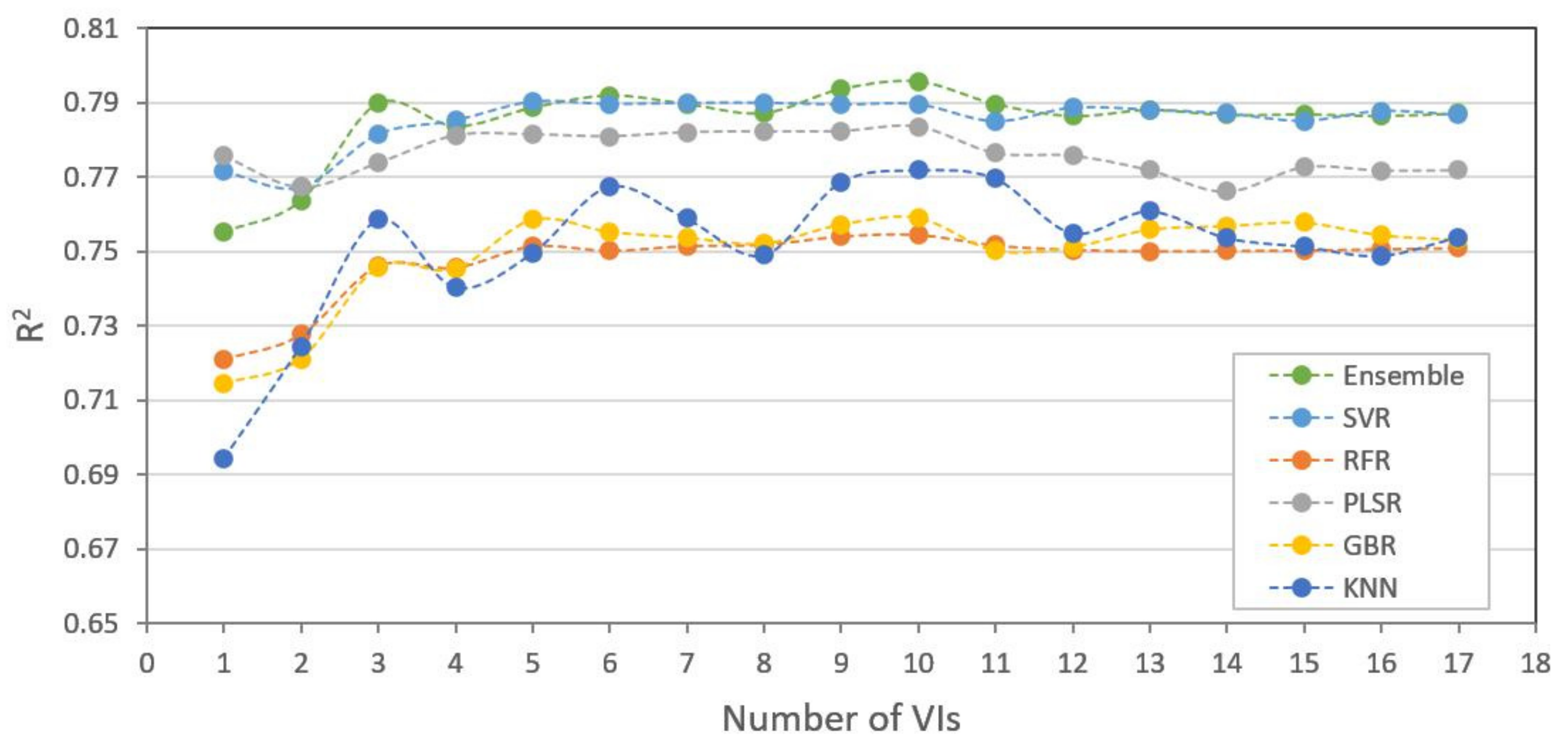
Model training accuracies as a function of the number of VIs derived from 0.045 m GSD multispectral data.
Figure A2.
Model training accuracies as a function of the number of VIs derived from 0.045 m GSD multispectral data.

Figure A3.
Model training accuracies as a function of the number of VIs derived from 0.045 m GSD RGB data.
Figure A3.
Model training accuracies as a function of the number of VIs derived from 0.045 m GSD RGB data.

References
- FAO. The Future of Food and Agriculture: Trends and Challenges; FAO: Rome, Italy, 2017. [Google Scholar]
- Weiss, M.; Jacob, F.; Duveiller, G. Remote sensing for agricultural applications: A meta-review. Remote Sens. Environ. 2020, 236, 111402. [Google Scholar] [CrossRef]
- Chason, J.W.; Baldocchi, D.D.; Huston, M.A. A Comparison of Direct and Indirect Methods for Estimating Forest Canopy Leaf-Area. Agric. For. Meteorol. 1991, 57, 107–128. [Google Scholar] [CrossRef]
- Clevers, J.G.P.W.; Kooistra, L.; van den Brande, M.M.M. Using Sentinel-2 Data for Retrieving LAI and Leaf and Canopy Chlorophyll Content of a Potato Crop. Remote Sens. 2017, 9, 405. [Google Scholar] [CrossRef] [Green Version]
- Towers, P.C.; Strever, A.; Poblete-Echeverría, C. Comparison of Vegetation Indices for Leaf Area Index Estimation in Vertical Shoot Positioned Vine Canopies with and without Grenbiule Hail-Protection Netting. Remote Sens. 2019, 11, 1073. [Google Scholar] [CrossRef] [Green Version]
- Vélez, S.; Barajas, E.; Rubio, J.A.; Vacas, R.; Poblete-Echeverría, C. Effect of Missing Vines on Total Leaf Area Determined by NDVI Calculated from Sentinel Satellite Data: Progressive Vine Removal Experiments. Appl. Sci. 2020, 10, 3612. [Google Scholar] [CrossRef]
- Watson, D.J. Comparative Physiological Studies on the Growth of Field Crops: I. Variation in Net Assimilation Rate and Leaf Area between Species and Varieties, and within and between Years. Ann. Bot. 1947, 11, 41–76. [Google Scholar] [CrossRef]
- Zheng, G.; Moskal, L.M. Retrieving Leaf Area Index (LAI) Using Remote Sensing: Theories, Methods and Sensors. Sensors 2009, 9, 2719–2745. [Google Scholar] [CrossRef] [Green Version]
- Hicks, S.K.; Lascano, R.J. Estimation of Leaf-Area Index for Cotton Canopies Using the Li-Cor Lai-2000 Plant Canopy Analyzer. Agron. J. 1995, 87, 458–464. [Google Scholar] [CrossRef]
- Weiss, M.; Baret, F.; Smith, G.J.; Jonckheere, I.; Coppin, P. Review of methods for in situ leaf area index (LAI) determination Part II. Estimation of LAI, errors and sampling. Agric. For. Meteorol. 2004, 121, 37–53. [Google Scholar] [CrossRef]
- Gates, D.J.; Westcott, M. A Direct Derivation of Miller Formula for Average Foliage Density. Aust. J. Bot. 1984, 32, 117–119. [Google Scholar] [CrossRef]
- Chen, J.M.; Cihlar, J. Plant Canopy Gap-Size Analysis Theory for Improving Optical Measurements of Leaf-Area Index. Appl. Opt. 1995, 34, 6211–6222. [Google Scholar] [CrossRef] [Green Version]
- Lang, A.R.G.; Mcmurtrie, R.E. Total Leaf Areas of Single Trees of Eucalyptus-Grandis Estimated from Transmittances of the Suns Beam. Agric. For. Meteorol. 1992, 58, 79–92. [Google Scholar] [CrossRef]
- Lang, A.R.G.; Xiang, Y.Q. Estimation of Leaf-Area Index from Transmission of Direct Sunlight in Discontinuous Canopies. Agric. For. Meteorol. 1986, 37, 229–243. [Google Scholar] [CrossRef]
- Breda, N.J.J. Ground-based measurements of leaf area index: A review of methods, instruments and current controversies. J. Exp. Bot. 2003, 54, 2403–2417. [Google Scholar] [CrossRef] [PubMed]
- Costa, J.D.; Coelho, R.D.; Barros, T.H.D.; Fraga, E.F.; Fernandes, A.L.T. Leaf area index and radiation extinction coefficient of a coffee canopy under variable drip irrigation levels. Acta Sci. Agron. 2019, 41, e42703. [Google Scholar] [CrossRef]
- Macfarlane, C.; Hoffman, M.; Eamus, D.; Kerp, N.; Higginson, S.; McMurtrie, R.; Adams, M. Estimation of leaf area index in eucalypt forest using digital photography. Agric. For. Meteorol. 2007, 143, 176–188. [Google Scholar] [CrossRef]
- Müller-Linow, M.; Wilhelm, J.; Briese, C.; Wojciechowski, T.; Schurr, U.; Fiorani, F. Plant Screen Mobile: An open-source mobile device app for plant trait analysis. Plant Methods 2019, 15, 2. [Google Scholar] [CrossRef] [Green Version]
- Easlon, H.M.; Bloom, A.J. Easy Leaf Area: Automated Digital Image Analysis for Rapid and Accurate Measurement of Leaf Area. Appl. Plant Sci. 2014, 2, 1400033. [Google Scholar] [CrossRef]
- Orlando, F.; Movedi, E.; Coduto, D.; Parisi, S.; Brancadoro, L.; Pagani, V.; Guarneri, T.; Confalonieri, R. Estimating Leaf Area Index (LAI) in Vineyards Using the PocketLAI Smart-App. Sensors 2016, 16, 2004. [Google Scholar] [CrossRef] [PubMed] [Green Version]
- De Bei, R.; Fuentes, S.; Gilliham, M.; Tyerman, S.; Edwards, E.; Bianchini, N.; Smith, J.; Collins, C. VitiCanopy: A Free Computer App to Estimate Canopy Vigor and Porosity for Grapevine. Sensors 2016, 16, 585. [Google Scholar] [CrossRef] [Green Version]
- Poblete-Echeverria, C.; Fuentes, S.; Ortega-Farias, S.; Gonzalez-Talice, J.; Yuri, J.A. Digital Cover Photography for Estimating Leaf Area Index (LAI) in Apple Trees Using a Variable Light Extinction Coefficient. Sensors 2015, 15, 2860–2872. [Google Scholar] [CrossRef] [PubMed] [Green Version]
- Turton, S.M. The relative distribution of photosynthetically active radiation within four tree canopies, Craigieburn Range, New Zealand. Aust. For. Res. 1985, 15, 383–394. [Google Scholar]
- Smith, F.W.; Sampson, D.A.; Long, J.N. Comparison of Leaf-Area Index Estimates from Tree Allometrics and Measured Light Interception. For. Sci. 1991, 37, 1682–1688. [Google Scholar]
- Smith, N.J. Estimating leaf area index and light extinction coefficients in stands of Douglas-fir (Pseudotsugamenziesii). Can. J. For. Res. 1993, 23, 317–321. [Google Scholar] [CrossRef]
- Pierce, L.L.; Running, S.W. Rapid Estimation of Coniferous Forest Leaf-Area Index Using a Portable Integrating Radiometer. Ecology 1988, 69, 1762–1767. [Google Scholar] [CrossRef]
- Jarvis, P.G.; Leverenz, J.W. Productivity of Temperate, Deciduous and Evergreen Forests, 1st ed.; Springer: Berlin, Germany, 1983; pp. 233–280. [Google Scholar]
- Vose, J.M.; Clinton, B.D.; Sullivan, N.H.; Bolstad, P.V. Vertical leaf area distribution, light transmittance, and application of the Beer-Lambert Law in four mature hardwood stands in the southern Appalachians. Can. J. For. Res. 1995, 25, 1036–1043. [Google Scholar] [CrossRef] [Green Version]
- Hassika, P.; Berbigier, P.; Bonnefond, J.M. Measurement and modelling of the photosynthetically active radiation transmitted in a canopy of maritime pine. Ann. Sci. For. 1997, 54, 715–730. [Google Scholar] [CrossRef] [Green Version]
- Turner, D.P.; Cohen, W.B.; Kennedy, R.E.; Fassnacht, K.S.; Briggs, J.M. Relationships between Leaf Area Index and Landsat TM Spectral Vegetation Indices across Three Temperate Zone Sites. Remote Sens. Environ. 1999, 70, 52–68. [Google Scholar] [CrossRef]
- Padalia, H.; Sinha, S.K.; Bhave, V.; Trivedi, N.K.; Kumar, A.S. Estimating canopy LAI and chlorophyll of tropical forest plantation (North India) using Sentinel-2 data. Adv. Space Res. 2020, 65, 458–469. [Google Scholar] [CrossRef]
- Sun, L.; Wang, W.Y.; Jia, C.; Liu, X.R. Leaf area index remote sensing based on Deep Belief Network supported by simulation data. Int. J. Remote Sens. 2021, 42, 7637–7661. [Google Scholar] [CrossRef]
- MODIS Web. Available online: http://modis.gsfc.nasa.gov/data/atbd/atbd_mod15.pdf (accessed on 3 November 2021).
- Baret, F.; Hagolle, O.; Geiger, B.; Bicheron, P.; Miras, B.; Huc, M.; Berthelot, B.; Nino, F.; Weiss, M.; Samain, O.; et al. LAI, fAPAR and fCover CYCLOPES global products derived from VEGETATION—Part 1: Principles of the algorithm. Remote Sens. Environ. 2007, 110, 275–286. [Google Scholar] [CrossRef] [Green Version]
- Sozzi, M.; Kayad, A.; Marinello, F.; Taylor, J.A.; Tisseyre, B. Comparing vineyard imagery acquired from Sentinel-2 and Unmanned Aerial Vehicle (UAV) platform. Oeno One 2020, 54, 189–197. [Google Scholar] [CrossRef] [Green Version]
- Zhang, R.; Jia, M.M.; Wang, Z.M.; Zhou, Y.M.; Wen, X.; Tan, Y.; Cheng, L.N. A Comparison of Gaofen-2 and Sentinel-2 Imagery for Mapping Mangrove Forests Using Object-Oriented Analysis and Random Forest. IEEE J. Sel. Top. Appl. Earth Obs. Remote Sens. 2021, 14, 4185–4193. [Google Scholar] [CrossRef]
- Kamal, M.; Sidik, F.; Prananda, A.R.A.; Mahardhika, S.A. Mapping Leaf Area Index of restored mangroves using WorldView-2 imagery in Perancak Estuary, Bali, Indonesia. Remote Sens. Appl. Soc. Environ. 2021, 23, 100567. [Google Scholar] [CrossRef]
- Kokubu, Y.; Hara, S.; Tani, A. Mapping Seasonal Tree Canopy Cover and Leaf Area Using Worldview-2/3 Satellite Imagery: A Megacity-Scale Case Study in Tokyo Urban Area. Remote Sens. 2020, 12, 1505. [Google Scholar] [CrossRef]
- Tian, J.Y.; Wang, L.; Li, X.J.; Gong, H.L.; Shi, C.; Zhong, R.F.; Liu, X.M. Comparison of UAV and WorldView-2 imagery for mapping leaf area index of mangrove forest. Int. J. Appl. Earth Obs. Geoinf. 2017, 61, 22–31. [Google Scholar] [CrossRef]
- Peng, X.S.; Han, W.T.; Ao, J.Y.; Wang, Y. Assimilation of LAI Derived from UAV Multispectral Data into the SAFY Model to Estimate Maize Yield. Remote Sens. 2021, 13, 1094. [Google Scholar] [CrossRef]
- Gong, Y.; Yang, K.L.; Lin, Z.H.; Fang, S.H.; Wu, X.T.; Zhu, R.S.; Peng, Y. Remote estimation of leaf area index (LAI) with unmanned aerial vehicle (UAV) imaging for different rice cultivars throughout the entire growing season. Plant Methods 2021, 17, 1–16. [Google Scholar] [CrossRef]
- Liu, Z.J.; Guo, P.J.; Liu, H.; Fan, P.; Zeng, P.Z.; Liu, X.Y.; Feng, C.; Wang, W.; Yang, F.Z. Gradient Boosting Estimation of the Leaf Area Index of Apple Orchards in UAV Remote Sensing. Remote Sens. 2021, 13, 3263. [Google Scholar] [CrossRef]
- Mathews, A.J.; Jensen, J.L.R. Visualizing and Quantifying Vineyard Canopy LAI Using an Unmanned Aerial Vehicle (UAV) Collected High Density Structure from Motion Point Cloud. Remote Sens. 2013, 5, 2164–2183. [Google Scholar] [CrossRef] [Green Version]
- Raj, R.; Walker, J.P.; Pingale, R.; Nandan, R.; Naik, B.; Jagarlapudi, A. Leaf area index estimation using top-of-canopy airborne RGB images. Int. J. Appl. Earth Obs. Geoinf. 2021, 96, 102282. [Google Scholar] [CrossRef]
- Yamaguchi, T.; Tanaka, Y.; Imachi, Y.; Yamashita, M.; Katsura, K. Feasibility of Combining Deep Learning and RGB Images Obtained by Unmanned Aerial Vehicle for Leaf Area Index Estimation in Rice. Remote Sens. 2021, 13, 84. [Google Scholar] [CrossRef]
- Yao, X.; Wang, N.; Liu, Y.; Cheng, T.; Tian, Y.C.; Chen, Q.; Zhu, Y. Estimation of Wheat LAI at Middle to High Levels Using Unmanned Aerial Vehicle Narrowband Multispectral Imagery. Remote Sens. 2017, 9, 1304. [Google Scholar] [CrossRef] [Green Version]
- Zhang, J.J.; Cheng, T.; Guo, W.; Xu, X.; Qiao, H.B.; Xie, Y.M.; Ma, X.M. Leaf area index estimation model for UAV image hyperspectral data based on wavelength variable selection and machine learning methods. Plant Methods 2021, 17, 1–14. [Google Scholar] [CrossRef] [PubMed]
- Zhu, X.; Li, C.; Tang, L.; Ma, L. Retrieval and scale effect analysis of LAI over typical farmland from UAV-based hyperspectral data. In Proceedings of the Remote Sensing for Agriculture, Ecosystems, and Hydrology XXI, Strasbourg, France, 9–11 September 2019. [Google Scholar]
- Tian, L.; Qu, Y.H.; Qi, J.B. Estimation of Forest LAI Using Discrete Airborne LiDAR: A Review. Remote Sens. 2021, 13, 2408. [Google Scholar] [CrossRef]
- Pastonchi, L.; Di Gennaro, S.F.; Toscano, P.; Matese, A. Comparison between satellite and ground data with UAV-based information to analyse vineyard spatio-temporal variability. Oeno One 2020, 54, 919–934. [Google Scholar] [CrossRef]
- Xiao, X.X.; Zhang, T.J.; Zhong, X.Y.; Shao, W.W.; Li, X.D. Support vector regression snow-depth retrieval algorithm using passive microwave remote sensing data. Remote Sens. Environ. 2018, 210, 48–64. [Google Scholar] [CrossRef]
- Tobias, R.D. An Introduction to Partial Least Squares Regression. In Proceedings of the SUGI Proceedings, Orlando, FL, USA, April 1995. [Google Scholar]
- Wold, S.; Sjostrom, M.; Eriksson, L. PLS-regression: A basic tool of chemometrics. Chemometr. Intell. Lab. Syst. 2001, 58, 109–130. [Google Scholar] [CrossRef]
- Breiman, L. Random forests. Mach. Learn. 2001, 45, 5–32. [Google Scholar] [CrossRef] [Green Version]
- Filippi, A.M.; Guneralp, I.; Randall, J. Hyperspectral remote sensing of aboveground biomass on a river meander bend using multivariate adaptive regression splines and stochastic gradient boosting. Remote Sens. Lett. 2014, 5, 432–441. [Google Scholar] [CrossRef]
- Adsule, P.G.; Karibasappa, G.S.; Banerjee, K.; Mundankar, K. Status and prospects of raisin industry in India. In Proceedings of the International Symposium on Grape Production and Processing, Baramati, India, 13 May 2008. [Google Scholar]
- Caruso, G.; Tozzini, L.; Rallo, G.; Primicerio, J.; Moriondo, M.; Palai, G.; Gucci, R. Estimating biophysical and geometrical parameters of grapevine canopies (’Sangiovese’) by an unmanned aerial vehicle (UAV) and VIS-NIR cameras. Vitis 2017, 56, 63–70. [Google Scholar]
- Gullo, G.; Branca, V.; Dattola, A.; Zappia, R.; Inglese, P. Effect of summer pruning on some fruit quality traits in Hayward kiwifruit. Fruits 2013, 68, 315–322. [Google Scholar] [CrossRef] [Green Version]
- Shiozaki, Y.; Kikuchi, T. Fruit Productivity as Related to Leaf-Area Index and Tree Vigor of Open-Center Apple-Trees Trained by Traditional Japanese System. J. Jpn. Soc. Hortic. Sci. 1992, 60, 827–832. [Google Scholar] [CrossRef] [Green Version]
- Grantz, D.A.; Zhang, X.J.; Metheney, P.D.; Grimes, D.W. Indirect Measurement of Leaf-Area Index in Pima Cotton (Gossypium-Barbadense L) Using a Commercial Gap Inversion Method. Agric. For. Meteorol. 1993, 67, 1–12. [Google Scholar] [CrossRef]
- Clevers, J.G.P.W.; Kooistra, L. Using Hyperspectral Remote Sensing Data for Retrieving Canopy Chlorophyll and Nitrogen Content. IEEE J. Sel. Top. Appl. Earth Obs. Remote Sens. 2012, 5, 574–583. [Google Scholar] [CrossRef]
- Beeri, O.; Netzer, Y.; Munitz, S.; Mintz, D.F.; Pelta, R.; Shilo, T.; Horesh, A.; Mey-tal, S. Kc and LAI Estimations Using Optical and SAR Remote Sensing Imagery for Vineyards Plots. Remote Sens. 2020, 12, 3478. [Google Scholar] [CrossRef]
- Zhou, X.; Yang, L.; Wang, W.; Chen, B. UAV Data as an Alternative to Field Sampling to Monitor Vineyards Using Machine Learning Based on UAV/Sentinel-2 Data Fusion. Remote Sens. 2021, 13, 457. [Google Scholar] [CrossRef]
- Hua, Y. Temperature Changes Characteristic of Turpan in Recent 60 Years. J. Arid Meteorol. 2012, 30, 630–634. [Google Scholar]
- Lv, T.; Wu, S.; Liu, Q.; Xia, S.; Ge, H.; Li, J. Variations of Extreme Temperature in Turpan City, Xinjiang during the Period of 1952–2013. Arid. Zone Res. 2018, 35, 606–614. [Google Scholar]
- Tetracam ADC Micro. Available online: https://tetracam.com/Products-ADC_Micro.htm (accessed on 10 October 2021).
- Sara, V.; Silvia, D.F.; Filippo, M.; Piergiorgio, M. Unmanned aerial vehicles and Geographical Information System integrated analysis of vegetation in Trasimeno Lake, Italy. Lakes Reserv. Sci. Policy Manag. Sustain. Use 2016, 21, 5–19. [Google Scholar]
- Candiago, S.; Remondino, F.; De Giglio, M.; Dubbini, M.; Gattelli, M. Evaluating Multispectral Images and Vegetation Indices for Precision Farming Applications from UAV Images. Remote Sens. 2015, 7, 4026–4047. [Google Scholar] [CrossRef] [Green Version]
- Hoffmann, C.M.; Blomberg, M. Estimation of leaf area index of Beta vulgaris L. based on optical remote sensing data. J. Agron. Crop. Sci. 2004, 190, 197–204. [Google Scholar]
- Gobron, N.; Pinty, B.; Verstraete, M.M.; Widlowski, J.L. Advanced vegetation indices optimized for up-coming sensors: Design, performance, and applications. IEEE Trans. Geosci. Remote Sens. 2000, 38, 2489–2505. [Google Scholar]
- Pichon, L.; Taylor, J.A.; Tisseyre, B. Using smartphone leaf area index data acquired in a collaborative context within vineyards in southern France. Oeno One 2020, 54, 123–130. [Google Scholar] [CrossRef]
- Tongson, E.J.; Fuentes, S.; Carrasco-Benavides, M.; Mora, M. Canopy architecture assessment of cherry trees by cover photography based on variable light extinction coefficient modelled using artificial neural networks. Acta Hortic. 2019, 1235, 183. [Google Scholar] [CrossRef]
- Fuentes, S.; Chacon, G.; Torrico, D.D.; Zarate, A.; Viejo, C.G. Spatial Variability of Aroma Profiles of Cocoa Trees Obtained through Computer Vision and Machine Learning Modelling: A Cover Photography and High Spatial Remote Sensing Application. Sensors 2019, 19, 3054. [Google Scholar] [CrossRef] [PubMed] [Green Version]
- Fuentes, S.; Palmer, A.R.; Taylor, D.; Zeppel, M.; Whitley, R.; Eamus, D. An automated procedure for estimating the leaf area index (LAI) of woodland ecosystems using digital imagery, MATLAB programming and its application to an examination of the relationship between remotely sensed and field measurements of LAI. Funct. Plant Biol. 2008, 35, 1070–1079. [Google Scholar] [CrossRef]
- Leblanc, S.G. Correction to the plant canopy gap-size analysis theory used by the Tracing Radiation and Architecture of Canopies instrument. Appl. Opt. 2002, 41, 7667–7670. [Google Scholar] [CrossRef]
- Kawashima, S.; Nakatani, M. An algorithm for estimating chlorophyll content in leaves using a video camera. Ann. Bot. 1998, 81, 49–54. [Google Scholar] [CrossRef] [Green Version]
- Schell, J.A. Monitoring vegetation systems in the great plains with ERTS. Nasa Spec. Publ. 1973, 351, 309. [Google Scholar]
- Vincini, M.; Frazzi, E.; D’Alessio, P. Comparison of narrow-band and broad-band vegetation indices for canopy chlorophyll density estimation in sugar beet. In Proceedings of the 6th European Conference on Precision Agriculture, Skiathos, Greece, 3–6 June 2007; Wageningen Academic Publishers: Wageningen, The Netherlands, 2007; pp. 189–196. [Google Scholar]
- Gitelson, A.A.; Gritz, Y.; Merzlyak, M.N. Relationships between leaf chlorophyll content and spectral reflectance and algorithms for non-destructive chlorophyll assessment in higher plant leaves. J. Plant Physiol. 2003, 160, 271–282. [Google Scholar] [CrossRef] [PubMed]
- Tucker, C.J.; Elgin, J.H.; Mcmurtrey, J.E.; Fan, C.J. Monitoring Corn and Soybean Crop Development with Hand-Held Radiometer Spectral Data. Remote Sens. Environ. 1979, 8, 237–248. [Google Scholar] [CrossRef]
- Kaufman, Y.J.; Tanre, D. Atmospherically Resistant Vegetation Index (Arvi) for Eos-Modis. IEEE Trans. Geosci. Remote Sens. 1992, 30, 261–270. [Google Scholar] [CrossRef]
- Jiang, Z.Y.; Huete, A.R.; Didan, K.; Miura, T. Development of a two-band enhanced vegetation index without a blue band. Remote Sens. Environ. 2008, 112, 3833–3845. [Google Scholar] [CrossRef]
- Wang, F.M.; Huang, J.F.; Tang, Y.L.; Wang, X.Z. New Vegetation Index and Its Application in Estimating Leaf Area Index of Rice. Rice Sci. 2007, 14, 195–203. [Google Scholar] [CrossRef]
- Zarco-Tejada, P.J.; Ustin, S.L.; Whiting, M.L. Temporal and spatial relationships between within-field yield variability in cotton and high-spatial hyperspectral remote sensing imagery. Agron. J. 2005, 97, 641–653. [Google Scholar] [CrossRef] [Green Version]
- Gitelson, A.A.; Kaufman, Y.J.; Stark, R.; Rundquist, D. Novel algorithms for remote estimation of vegetation fraction. Remote Sens. Environ. 2002, 80, 76–87. [Google Scholar] [CrossRef] [Green Version]
- Boegh, E.; Soegaard, H.; Broge, N.; Hasager, C.B.; Jensen, N.O.; Schelde, K.; Thomsen, A. Airborne multispectral data for quantifying leaf area index, nitrogen concentration, and photosynthetic efficiency in agriculture. Remote Sens. Environ. 2002, 81, 179–193. [Google Scholar] [CrossRef]
- Sims, D.A.; Gamon, J.A. Estimation of vegetation water content and photosynthetic tissue area from spectral reflectance: A comparison of indices based on liquid water and chlorophyll absorption features. Remote Sens. Environ. 2003, 84, 526–537. [Google Scholar] [CrossRef]
- Zarco-Tejada, P.J.; Berjon, A.; Lopez-Lozano, R.; Miller, J.R.; Martin, P.; Cachorro, V.; Gonzalez, M.R.; de Frutos, A. Assessing vineyard condition with hyperspectral indices: Leaf and canopy reflectance simulation in a row-structured discontinuous canopy. Remote Sens. Environ. 2005, 99, 271–287. [Google Scholar] [CrossRef]
- Woebbecke, D.M.; Meyer, G.E.; Vonbargen, K.; Mortensen, D.A. Color Indexes for Weed Identification under Various Soil, Residue, and Lighting Conditions. Trans. ASAE 1995, 38, 259–269. [Google Scholar] [CrossRef]
- Escadafal, R.; Belghith, A.; Moussa, H.B. Indices spectraux pour la teledetection de la degradation des milieux naturels en tunisie aride. In Proceedings of the 6th International Symposium on Physical Measurements and Signatures in Remote Sensing, Val-d’Isère, France, 17–24 January 1994; pp. 253–259. [Google Scholar]
- Rivera-Caicedo, J.P.; Verrelst, J.; Munoz-Mari, J.; Camps-Valls, G.; Moreno, J. Hyperspectral dimensionality reduction for biophysical variable statistical retrieval. ISPRS J. Photogramm. Remote Sens. 2017, 132, 88–101. [Google Scholar] [CrossRef]
- Karegowda, A.G.; Manjunath, A.S.; Jayaram, M.A. Comparative study of attribute selection using gain ratio and correlation based feature selection. Int. J. Inf. Manag. 2010, 2, 271–277. [Google Scholar]
- Guyon, I.; Elisseeff, A. An introduction to variable and feature selection. J. Mach. Learn. Res. 2003, 3, 1157–1182. [Google Scholar]
- Zhao, J.Q.; Karimzadeh, M.; Masjedi, A.; Wang, T.J.; Zhang, X.W.; Crawford, M.M.; Ebert, D.S. FeatureExplorer: Interactive Feature Selection and Exploration of Regression Models for Hyperspectral Images. In Proceedings of the 2019 IEEE Visualization Conference (VIS), Vancouver, BC, Canada, 20–25 October 2019. [Google Scholar]
- Moghimi, A.; Yang, C.; Marchetto, P.M. Ensemble Feature Selection for Plant Phenotyping: A Journey From Hyperspectral to Multispectral Imaging. IEEE Access 2018, 6, 56870–56884. [Google Scholar] [CrossRef]
- Feng, L.W.; Zhang, Z.; Ma, Y.C.; Du, Q.Y.; Williams, P.; Drewry, J.; Luck, B. Alfalfa Yield Prediction Using UAV-Based Hyperspectral Imagery and Ensemble Learning. Remote Sens. 2020, 12, 2028. [Google Scholar] [CrossRef]
- Sylvester, E.V.A.; Bentzen, P.; Bradbury, I.R.; Clement, M.; Pearce, J.; Horne, J.; Beiko, R.G. Applications of random forest feature selection for fine-scale genetic population assignment. Evol. Appl. 2018, 11, 153–165. [Google Scholar] [CrossRef]
- Jin-Lei, L.I.; Zhu, X.L.; Zhu, H.Y. A Clustering Ensembles Algorithm Based on Voting Strategy. Comput. Simul. 2008, 3, 126–128. [Google Scholar]
- Lan, Y.B.; Huang, Z.X.; Deng, X.L.; Zhu, Z.H.; Huang, H.S.; Zheng, Z.; Lian, B.Z.; Zeng, G.L.; Tong, Z.J. Comparison of machine learning methods for citrus greening detection on UAV multispectral images. Comput. Electron. Agr. 2020, 171, 105234. [Google Scholar] [CrossRef]
- Azadbakht, M.; Ashourloo, D.; Aghighi, H.; Radiom, S.; Alimohammadi, A. Wheat leaf rust detection at canopy scale under different LAI levels using machine learning techniques. Comput. Electron. Agr. 2019, 156, 119–128. [Google Scholar] [CrossRef]
- Bahat, I.; Netzer, Y.; Grunzweig, J.M.; Alchanatis, V.; Peeters, A.; Goldshtein, E.; Ohana-Levi, N.; Ben-Gal, A.; Cohen, Y. In-Season Interactions between Vine Vigor, Water Status and Wine Quality in Terrain-Based Management-Zones in a ‘Cabernet Sauvignon’ Vineyard. Remote Sens. 2021, 13, 1636. [Google Scholar] [CrossRef]
- Yang, K.L.; Gong, Y.; Fang, S.H.; Duan, B.; Yuan, N.G.; Peng, Y.; Wu, X.T.; Zhu, R.S. Combining Spectral and Texture Features of UAV Images for the Remote Estimation of Rice LAI throughout the Entire Growing Season. Remote Sens. 2021, 13, 3001. [Google Scholar] [CrossRef]
- Susantoro, T.M.; Wikantika, K.; Saepuloh, A.; Harsolumakso, A.H. Selection of vegetation indices for mapping the sugarcane condition around the oil and gas field of North West Java Basin, Indonesia. Iop. C Ser. Earth Environ. 2018, 149, 012001. [Google Scholar] [CrossRef] [Green Version]
- Chen, Z.L.; Jia, K.; Xiao, C.C.; Wei, D.D.; Zhao, X.; Lan, J.H.; Wei, X.Q.; Yao, Y.J.; Wang, B.; Sun, Y.; et al. Leaf Area Index Estimation Algorithm for GF-5 Hyperspectral Data Based on Different Feature Selection and Machine Learning Methods. Remote Sens. 2020, 12, 2110. [Google Scholar] [CrossRef]
- Grabska, E.; Frantz, D.; Ostapowicz, K. Evaluation of machine learning algorithms for forest stand species mapping using Sentinel-2 imagery and environmental data in the Polish Carpathians. Remote Sens. Environ. 2020, 251, 112103. [Google Scholar] [CrossRef]
- Leuning, R.; Hughes, D.; Daniel, P.; Coops, N.C.; Newnham, G. A multi-angle spectrometer for automatic measurement of plant canopy reflectance spectra. Remote Sens. Environ. 2006, 103, 236–245. [Google Scholar] [CrossRef]
Figure 1.
Location of study area, birds eye view of a vineyard, and a scene below the pergola.

Figure 2.
Calculation procedure of true LAI values: (a) collect all leaves inside the rectangular frame; (b) put leaves on A2 paper and take photo with RGB camera; (c) distinguish the leaves and calculate the area.
Figure 2.
Calculation procedure of true LAI values: (a) collect all leaves inside the rectangular frame; (b) put leaves on A2 paper and take photo with RGB camera; (c) distinguish the leaves and calculate the area.

Figure 3.
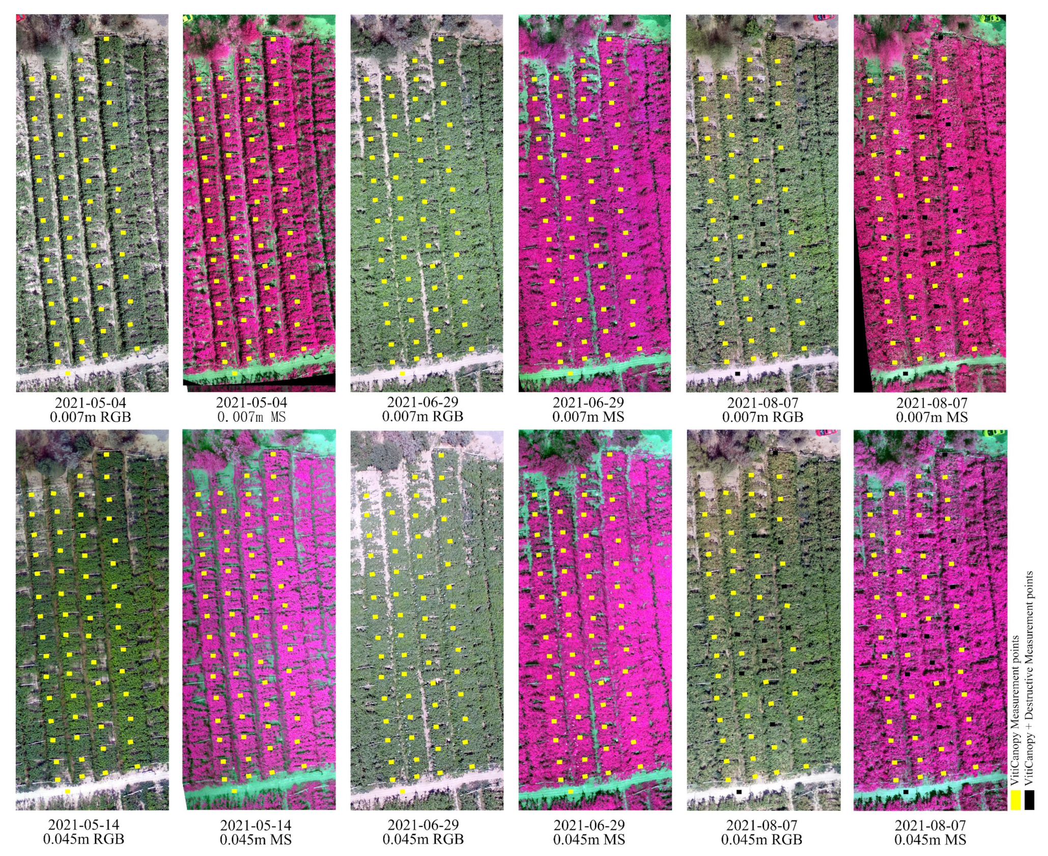
Locations of VitiCanopy and destructive sampling measurements. Ortho mosaiced RGB and false color images of sampled vineyard with 0.007 m and 0.045 m GSD on different dates. The yellow and black rectangles refer to 0.80 m × 0.90 m regions which were measured using VitiCanopy and black rectangles refer to the plots of the destructive sampling measurements.
Figure 3.
Locations of VitiCanopy and destructive sampling measurements. Ortho mosaiced RGB and false color images of sampled vineyard with 0.007 m and 0.045 m GSD on different dates. The yellow and black rectangles refer to 0.80 m × 0.90 m regions which were measured using VitiCanopy and black rectangles refer to the plots of the destructive sampling measurements.

Figure 4.
An overview of workflow in this study, and datasets used for constructing models.

Figure 5.
Linear and exponential correlations of light extinction coefficient (km), which were calculated from true LAI values, and fraction of foliage cover ().
Figure 5.
Linear and exponential correlations of light extinction coefficient (km), which were calculated from true LAI values, and fraction of foliage cover ().

Figure 6.
The relationship between true and VitiCanopy calculated LAI (LAI_viti) values before and after optimization of k value. The default and optimized k values were 0.70 and 0.41 separately.
Figure 6.
The relationship between true and VitiCanopy calculated LAI (LAI_viti) values before and after optimization of k value. The default and optimized k values were 0.70 and 0.41 separately.

Figure 7.
Pearson’s correlation coefficients between LAI_viti and vegetation indices (VIs) derived from UAV multispectral images from 0.007 m (n = 148) and 0.045 m (n = 145) GSD data.
Figure 7.
Pearson’s correlation coefficients between LAI_viti and vegetation indices (VIs) derived from UAV multispectral images from 0.007 m (n = 148) and 0.045 m (n = 145) GSD data.

Figure 8.
Pearson’s correlation coefficients between LAI_viti and VIs derived from UAV RGB images of 0.007 m (n = 148) and 0.045 m (n = 145) GSD data.
Figure 8.
Pearson’s correlation coefficients between LAI_viti and VIs derived from UAV RGB images of 0.007 m (n = 148) and 0.045 m (n = 145) GSD data.

Figure 9.
Statistics of VI rankings in 300 experiments using 0.007 m GSD data from (a) multispectral sensor and (b) RGB sensor.
Figure 9.
Statistics of VI rankings in 300 experiments using 0.007 m GSD data from (a) multispectral sensor and (b) RGB sensor.

Figure 10.
Statistics of VI rankings in 300 experiments using 0.045 m GSD data from (a) multispectral sensor and (b) RGB sensor.
Figure 10.
Statistics of VI rankings in 300 experiments using 0.045 m GSD data from (a) multispectral sensor and (b) RGB sensor.

Figure 11.
Model training accuracies as a function of the number of VIs derived from 0.007 m GSD multispectral data.
Figure 11.
Model training accuracies as a function of the number of VIs derived from 0.007 m GSD multispectral data.

Figure 12.
Scatter plots of predicted and true LAI values from (a) SVR, (b) RFR, (c) PLSR, (d) GBR, (e) KNN and (f) ensemble model for (1) 0.007 m GSD MS dataset, (2) 0.007 m GSD RGB dataset, (3) 0.045 m GSD MS dataset and (4) 0.045 m GSD RGB dataset.
Figure 12.
Scatter plots of predicted and true LAI values from (a) SVR, (b) RFR, (c) PLSR, (d) GBR, (e) KNN and (f) ensemble model for (1) 0.007 m GSD MS dataset, (2) 0.007 m GSD RGB dataset, (3) 0.045 m GSD MS dataset and (4) 0.045 m GSD RGB dataset.

Figure 13.
Performance of different models in 0.007 m GSD MS datasets with (a) all VIs, (b) three band data and (c) selected VIs, and RGB datasets with (d) all VIs, (e) three band data and (f) selected VIs.
Figure 13.
Performance of different models in 0.007 m GSD MS datasets with (a) all VIs, (b) three band data and (c) selected VIs, and RGB datasets with (d) all VIs, (e) three band data and (f) selected VIs.

Figure 14.
Performance of different models in 0.045 m GSD MS dataset with (a) all VIs, (b) three band data and (c) selected VIs, and RGB datasets with (d) all VIs, (e) three band data and (f) selected VIs.
Figure 14.
Performance of different models in 0.045 m GSD MS dataset with (a) all VIs, (b) three band data and (c) selected VIs, and RGB datasets with (d) all VIs, (e) three band data and (f) selected VIs.

Table 1.
Sampling date and corresponding growing seasons for true leaf area index (LAI), VitiCanopy and unmanned aerial vehicle (UAV) missions.
Table 1.
Sampling date and corresponding growing seasons for true leaf area index (LAI), VitiCanopy and unmanned aerial vehicle (UAV) missions.
| Mission Date | Growth Period of Vine | Data Type | Flight Height | GSD |
|---|---|---|---|---|
| 4 May | Blooming stage | VitiCanopy, UAV data | 17 m | 0.007 m |
| 14 May | Fruit setting stage | VitiCanopy, UAV data | 100 m | 0.045 m |
| 29 June | Veraison stage | VitiCanopy, UAV data | 17 m, 100 m | 0.007 m, 0.045 m |
| 7 August | Post-harvest stage | True LAI, VitiCanopy, UAV data | 17 m, 91 m | 0.007 m, 0.045 m |
Note: UAV data includes both red, blue and green (RGB) and multispectral data; GSD refers to the ground sample distance (spatial resolution).
Table 2.
Number of samples in each dataset.
| Dataset | Number of Samples |
|---|---|
| 0.007 m GSD MS | 148 |
| 0.007 m GSD RGB | 145 |
| 0.045 m GSD MS | 148 |
| 0.045 m GSD RGB | 145 |
Table 3.
Vegetation indices used in this study.
| Vegetation Index Name | Abbrev. | Formula | Used Sensor | Source |
|---|---|---|---|---|
| Near Infrared | NIR | NIR | MS | |
| Red | R | R | MS, RGB | [76] |
| Green | G | G | MS, RGB | [76] |
| Blue | B | B | RGB | [76] |
| Normalized Differential Vegetation Index | NDVI | (NIR − R)/(NIR + R) | MS | [77] |
| Chlorophyll Vegetation Index | CVI | NIR∗R/G2 | MS | [78] |
| Chlorophyll Index Green | CIgreen | (NIR/G) − 1 | MS | [79] |
| Green Difference Vegetation Index | GDVI | NIR − G | MS | [80] |
| Enhanced Vegetation Index 1 | EVI1 | 2.4∗(NIR − R)/(NIR + R + 1) | MS | [81] |
| Enhanced Vegetation Index 2 | EVI2 | 2.5∗(NIR − R)/(NIR + 2.4*R + 1) | MS | [82] |
| Green-Red NDVI | GRNDVI | (NIR − R − G)/(NIR + R + G) | MS | [83] |
| Green NDVI | GNDVI | (NIR − G)/(NIR + G) | MS | [84] |
| Green Ratio Vegetation Index | GRVI | NIR/G | MS | [85] |
| Difference Vegetation Index | DVI | NIR/R | MS | [86] |
| Log Ratio | LogR | Log(NIR/R) | MS | |
| Soil Adjusted Vegetation Index | SAVI | (1 + L)(NIR − R)/(NIR + R + L) | MS | [87] |
| Simple Ratio Green to Red | GtoR | G/R | MS, RGB | |
| Simple Ratio Blue to Green | BtoG | B/G | RGB | [88] |
| Simple Ratio Blue to Red | BtoR | B/R | RGB | [88] |
| Simple difference of green and blue | GmB | G − B | RGB | [76] |
| Simple difference of red and blue | RmB | R − B | RGB | [76] |
| Simple difference of red and green | RmG | R − G | MS, RGB | |
| Simple Ratio of Green and Red + Blue | tGmRmB | 2G − R − B | RGB | [89] |
| Mean RGB | RGBto3 | (R + G + B)/3 | RGB | |
| Red Percentage Index | RtoRGB | R/(R + G + B) | RGB | [76] |
| Green Percentage Index | GtoRGB | G/(R + G + B) | RGB | [76] |
| Blue Percentage Index | BtoRGB | B/(R + G + B) | RGB | [76] |
| Normalized Green-Red Index | NGR | (G − R)/(G + R) | RGB | [76,85] |
| Normalized Red-Blue Index | NRB | (R − B)/(R + B) | RGB | [76] |
| Normalized Green-Blue Index | NGB | (G − B)/(G + B) | RGB | [76] |
| Green Leaf Index | GLI | (2G − R − B)/(2G + R + B) | RGB | [70] |
| Coloration Index | CI | (Red - Blue)/Red | RGB | [90] |
Note: MS refers to the multispectral sensor, and RGB refers to the RGB camera of the UAV.
Table 4.
Models for light extinction coefficient as a function of fractions of foliage cover (), and the goodness of fit (R2) and root mean square errors (RMSE) of those models.
Table 4.
Models for light extinction coefficient as a function of fractions of foliage cover (), and the goodness of fit (R2) and root mean square errors (RMSE) of those models.
| Model Type | Equation | R2 | RMSE |
|---|---|---|---|
| Linear | + 0.17 | 0.57 | 0.0591 |
| Exponential | 0.50 | 0.65 | 0.0593 |
Table 5.
Test accuracies including mean and standard deviation of five base models and an ensemble model trained on the 0.007 m GSD MS dataset in a different number of VIs (n = 148).
Table 5.
Test accuracies including mean and standard deviation of five base models and an ensemble model trained on the 0.007 m GSD MS dataset in a different number of VIs (n = 148).
| ML Methods | Using All 17 VIs | Using Selected 5 VIs | Using 3 Bands | ||||||
|---|---|---|---|---|---|---|---|---|---|
| R2 | RMSE | MAE | R2 | RMSE | MAE | R2 | RMSE | MAE | |
| SVR | 0.872 (0.022) | 0.466 (0.030) | 0.372 (0.021) | 0.864 (0.029) | 0.479 (0.043) | 0.385 (0.038) | 0.807 (0.026) | 0.572 (0.026) | 0.466 (0.038) |
| RFR | 0.864 (0.009) | 0.481 (0.013) | 0.399 (0.019) | 0.879 (0.015) | 0.455 (0.022) | 0.373 (0.028) | 0.742 (0.045) | 0.661 (0.051) | 0.556 (0.054) |
| PLSR | 0.880 (0.020) | 0.451 (0.028) | 0.366 (0.027) | 0.869 (0.026) | 0.469 (0.039) | 0.384 (0.036) | 0.822 (0.041) | 0.547 (0.050) | 0.451 (0.052) |
| GBR | 0.860 (0.011) | 0.489 (0.018) | 0.398 (0.033) | 0.879 (0.016) | 0.454 (0.025) | 0.368 (0.034) | 0.759 (0.059) | 0.636 (0.073) | 0.524 (0.084) |
| KNN | 0.856 (0.033) | 0.492 (0.054) | 0.404 (0.046) | 0.850 (0.014) | 0.506 (0.018) | 0.413 (0.031) | 0.773 (0.032) | 0.621 (0.033) | 0.508 (0.043) |
| Ensemble | 0.887 (0.013) | 0.438 (0.018) | 0.358 (0.027) | 0.889 (0.018) | 0.434 (0.030) | 0.354 (0.039) | 0.830 (0.031) | 0.536 (0.042) | 0.449 (0.053) |
Table 6.
Performances of base and ensemble models in LAI prediction under different GSD and sensor data.
Table 6.
Performances of base and ensemble models in LAI prediction under different GSD and sensor data.
| Model | Metrics | 0.007 m GSD MS | 0.007 m GSD RGB | 0.045 m GSD MS | 0.045 m GSD RGB |
|---|---|---|---|---|---|
| SVR | R2 | 0.864 | 0.818 | 0.790 | 0.438 |
| RMSE | 0.479 | 0.556 | 0.590 | 0.952 | |
| MAE | 0.385 | 0.407 | 0.449 | 0.678 | |
| RFR | R2 | 0.879 | 0.791 | 0.754 | 0.676 |
| RMSE | 0.455 | 0.598 | 0.635 | 0.734 | |
| MAE | 0.373 | 0.470 | 0.499 | 0.611 | |
| PLSR | R2 | 0.869 | 0.820 | 0.783 | 0.490 |
| RMSE | 0.469 | 0.552 | 0.598 | 0.921 | |
| MAE | 0.384 | 0.432 | 0.459 | 0.695 | |
| GBR | R2 | 0.879 | 0.788 | 0.758 | 0.708 |
| RMSE | 0.454 | 0.602 | 0.630 | 0.697 | |
| MAE | 0.368 | 0.470 | 0.492 | 0.568 | |
| KNN | R2 | 0.850 | 0.772 | 0.772 | 0.539 |
| RMSE | 0.506 | 0.623 | 0.614 | 0.872 | |
| MAE | 0.413 | 0.492 | 0.479 | 0.720 | |
| Ensemble | R2 | 0.889 | 0.825 | 0.796 | 0.637 |
| RMSE | 0.434 | 0.547 | 0.581 | 0.775 | |
| MAE | 0.354 | 0.422 | 0.452 | 0.626 |
Publisher’s Note: MDPI stays neutral with regard to jurisdictional claims in published maps and institutional affiliations. |
© 2022 by the authors. Licensee MDPI, Basel, Switzerland. This article is an open access article distributed under the terms and conditions of the Creative Commons Attribution (CC BY) license (https://creativecommons.org/licenses/by/4.0/).
Share and Cite
MDPI and ACS Style
Ilniyaz, O.; Kurban, A.; Du, Q. Leaf Area Index Estimation of Pergola-Trained Vineyards in Arid Regions Based on UAV RGB and Multispectral Data Using Machine Learning Methods. Remote Sens. 2022, 14, 415. https://doi.org/10.3390/rs14020415
AMA Style
Ilniyaz O, Kurban A, Du Q. Leaf Area Index Estimation of Pergola-Trained Vineyards in Arid Regions Based on UAV RGB and Multispectral Data Using Machine Learning Methods. Remote Sensing. 2022; 14(2):415. https://doi.org/10.3390/rs14020415
Chicago/Turabian StyleIlniyaz, Osman, Alishir Kurban, and Qingyun Du. 2022. "Leaf Area Index Estimation of Pergola-Trained Vineyards in Arid Regions Based on UAV RGB and Multispectral Data Using Machine Learning Methods" Remote Sensing 14, no. 2: 415. https://doi.org/10.3390/rs14020415
Note that from the first issue of 2016, this journal uses article numbers instead of page numbers. See further details here.