
Variational-Scale Segmentation for Multispectral Remote-Sensing Images Using Spectral Indices

Department of Geographic Information Science, Hohai University, Xikang Road No. 1, Nanjing 210024, China
*
Author to whom correspondence should be addressed.
Remote Sens. 2022, 14(2), 326; https://doi.org/10.3390/rs14020326
Submission received: 26 October 2021
/
Revised: 22 November 2021
/
Accepted: 24 November 2021
/
Published: 11 January 2022
Abstract
:Many studies have focused on performing variational-scale segmentation to represent various geographical objects in high-resolution remote-sensing images. However, it remains a significant challenge to select the most appropriate scales based on the geographical-distribution characteristics of ground objects. In this study, we propose a variational-scale multispectral remote-sensing image segmentation method using spectral indices. Real scenes in remote-sensing images contain different types of land cover with different scales. Therefore, it is difficult to segment images optimally based on the scales of different ground objects. To guarantee image segmentation of ground objects with their own scale information, spectral indices that can be used to enhance some types of land cover, such as green cover and water bodies, were introduced into marker generation for the watershed transformation. First, a vector field model was used to determine the gradient of a multispectral remote-sensing image, and a marker was generated from the gradient. Second, appropriate spectral indices were selected, and the kernel density estimation was used to generate spectral-index marker images based on the analysis of spectral indices. Third, a series of mathematical morphology operations were used to obtain a combined marker image from the gradient and the spectral index markers. Finally, the watershed transformation was used for image segmentation. In a segmentation experiment, an optimal threshold for the spectral-index-marker generation method was identified. Additionally, the influence of the scale parameter was analyzed in a segmentation experiment based on a five-subset dataset. The comparative results for the proposed method, the commonly used watershed segmentation method, and the multiresolution segmentation method demonstrate that the proposed method yielded multispectral remote-sensing images with much better performance than the other methods.
1. Introduction
Based on the development of remote-sensing technology, high-spatial-resolution remotely sensed images, such as IKONOS, Quickbird, GeoEye-I, and WorldView, are available for use in environmental monitoring, management, and protection works. High spatial resolution facilitates the retrieval of the structural details of geographical objects for land cover/use mapping and monitoring. However, high spatial resolution can generate salt-and-pepper noise effects in pixel-based image-analysis methods. Therefore, the object-based image analysis (OBIA) technique, which provides information on images based on meaningful objects, was proposed for high-spatial-resolution remote-sensing image analysis. The main prerequisite for OBIA is image segmentation, which has already been recognized as a valuable approach for identifying regions instead of pixels as feature carriers, which are then used for classification [1,2,3,4,5,6,7]. In addition to the use of remote-sensing data with high spatial resolution, the OBIA technique has also been used for gathering remote-sensing images with lower spatial resolutions, such as ASTER and TM data [8,9,10,11,12].
The goal of an image segmentation algorithm is to divide an image into meaningful separate regions that are homogeneous with respect to one or more properties, such as texture, color, or brightness [13]. These properties fall into four categories: characteristic feature thresholds or clusters, edge detection, region growing or extraction, and iterative pixel classification [14]. An image-segmentation algorithm may belong to two or more of these categories. Many image-segmentation algorithms have been proposed in the field of computer vision over the past several decades. There are also many applications of image segmentation in remote sensing, such as watershed transformation [15,16], region growing [17,18,19], Markov random field models [20,21], and fuzzy image regions [22].
However, a major difficulty in processing natural images is that changes can and do occur over a wide range of scales [23,24]. Remote-sensing images are used to represent the natural geographical world. Therefore, it is difficult to obtain optimal image-segmentation results according to the different scales of ground objects [25]. The multi-scale segmentation strategy is widely used to handle the difficulty of wide scale ranges [26], but the automatic selection of optimal segmentation scales for successive analysis remains a significant challenge [27] for which unsupervised segmentation evaluation methods are widely adopted [28,29,30].
Originally, many efforts were made to select a single optimal segmentation scale by combining intra-segment homogeneity and inter-segment heterogeneity [31,32,33,34,35] or by considering abrupt changes in homogeneity in terms of all segments [36,37,38]. However, global optimal segmentation scales still contain segments that are either too coarse or too fine because segmentation based on a single global scale parameter makes it difficult to separate various geographical objects [33].
To overcome this problem, the concept of deriving locally adaptive scale parameters has received significant attention in recent years with the goal of selecting optimal remote-sensing image segmentation scale parameters for different regions or objects [39]. There are two main types of automatic methods for determining local scale parameters. One is to tune a global optimal scale parameter locally according to the heterogeneity of local structures [40,41,42,43]. The other is to first partition an image into different regions or landscapes and then determine the optimal segmentation scale for each region using a global evaluation measure [44,45]. Overall, the segmentation performance of such methods depends on the effectiveness of the global evaluation measure. Additionally, locally optimized scale parameters are mainly designed for different objects without considering the spectral and spatial characteristics of different land-cover categories. We propose the utilization of spectral indexes for determining the optimal segmentation scales of different land-cover categories in the watershed transformation framework.
Because spectral indices from multispectral remote-sensing data such as the normalized difference vegetation index (NDVI) and the normalized difference water index (NDWI), which are used to enhance the information of some specific ground objects, may not be influenced by the interior textures of geographical objects and can maintain consistency between segmentation results for agminated land cover (e.g., vegetation, water, and snow), as well as the outlines of real ground objects in a natural scene, they can be used to generate markers for variational-scale segmentation. The watershed transformation [46,47] is a widely used method in which the quality of the markers directly determines the segmentation scales. Therefore, final segmentation quality depends on marker generation. If markers can be generated according to the self-scales of geographical objects, then the watershed transformation can be used to obtain variational-scale segmentation results for geographic objects. Spectral-index-based markers can also help to overcome the phenomenon of over-segmentation because they are sensitive to irrelevant local minima generated by gradients. Overall, remote-sensing images can provide more-complex scenes for watershed-transformation-based segmentation compared to other images, such as medical, finger, eye, and facial images.
In this study, the main goal was to use the spectral indices of multispectral remote-sensing images to develop a scale-variable watershed method for multispectral remote-sensing image segmentation based on watershed transformation. First, multispectral gradient-based markers were obtained using a vector field model (VFM) for multispectral remote-sensing images. Second, a novel marker generation method was applied to determine corresponding spectral indices based on kernel density estimation (KDE). Third, mathematical morphology was used to integrate gradient information and spectral indices into a single combined marker. Next, the final combined marker was used with the watershed transformation method for multispectral remote-sensing image segmentation. Finally, high-spatial-resolution multispectral remote-sensing datasets were used as experimental data to validate the proposed segmentation method.
The remainder of this article is organized as follows. Section 2 discusses marker generation for a multispectral gradient using a vector field model, marker generation using spectral indices, and image segmentation based on a combination of markers from gradient and spectral indices. In Section 3, we introduce experimental data, evaluation measures, and our experimental setup. Section 4 describes experiments on two high-resolution multispectral remote-sensing images. The segmentation results and gradient-marker-controlled watershed transformation for each image are compared. Section 5 summarizes our results and presents conclusions.
2. Study Area and Data
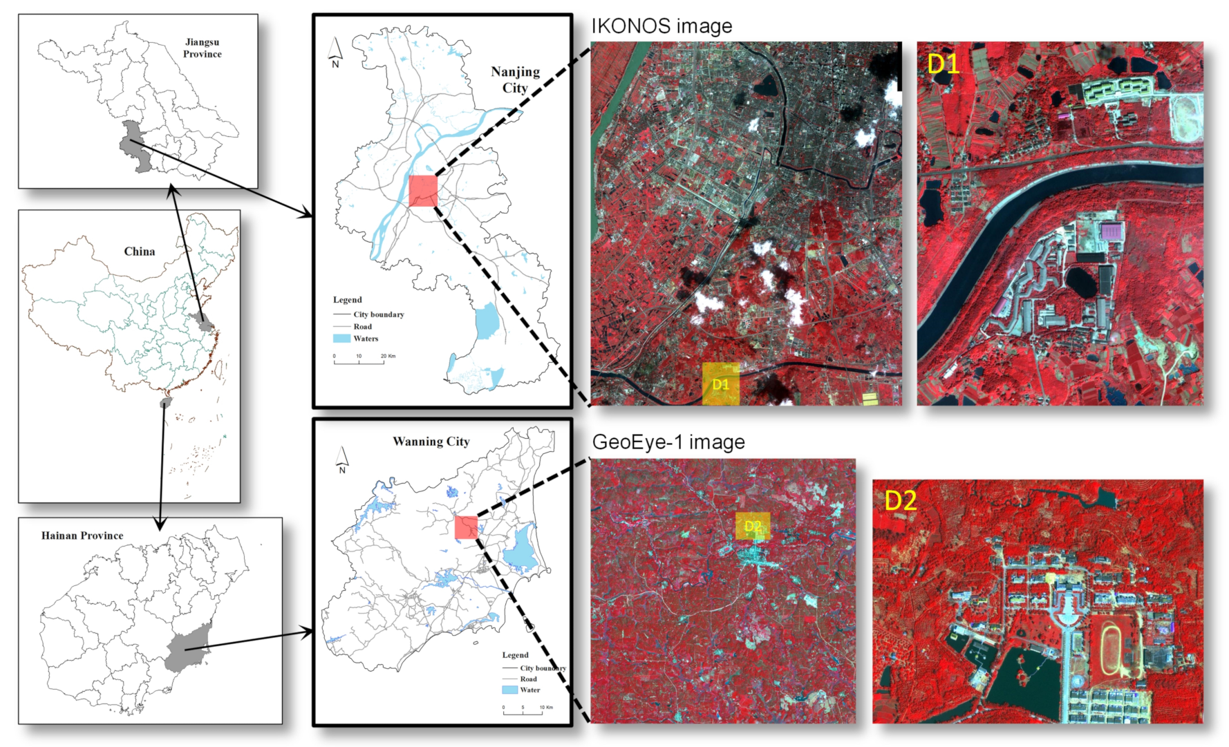
The study area is located in Nanjing City, Jiangsu Province and Wanning City, Hainan Province, China, as shown in Figure 1. As one of the four garden cities in China, Nanjing City has an abundance of urban green spaces and water bodies. Wanning City has a tropical monsoon marine climate with a large amount of vegetative cover and water bodies. Additionally, because China has experienced rapid economic development over the past 40 y, there are many man-made structures mixed with natural landscapes in the study area, providing good study samples for our experiments.
An IKONOS image covering an area of 108 km over Nanjing City and a GeoEye-I image covering an area 49 km in Wanning city were used as our experimental dataset. These two images consist of four spectral bands: blue, green, red, and near-infrared. The spatial resolutions of the multispectral bands and panchromatic band of the IKONOS image are 4.0 m and 1.0 m, respectively. A subset image called D1 with a 1.08 km × 1.37 km area was used to represent the segmentation results. There is significant vegetative cover, watery areas, and built-up land cover in the IKONOS image. The spatial resolution of the multispectral bands and panchromatic band of the GeoEye-I image are 1.64 m and 0.41 m, respectively. A subset image called D2 with a 0.9 km × 0.66 km area was used to represent the segmentation results. The GeoEye-1 image mainly contains vegetative cover with smaller areas of residential neighborhoods and watery cover. Additionally, the vegetative cover can be divided into farmland, shrubbery, and forestry, which are suitable categories for our experiments.
3. Methodology
3.1. Overview
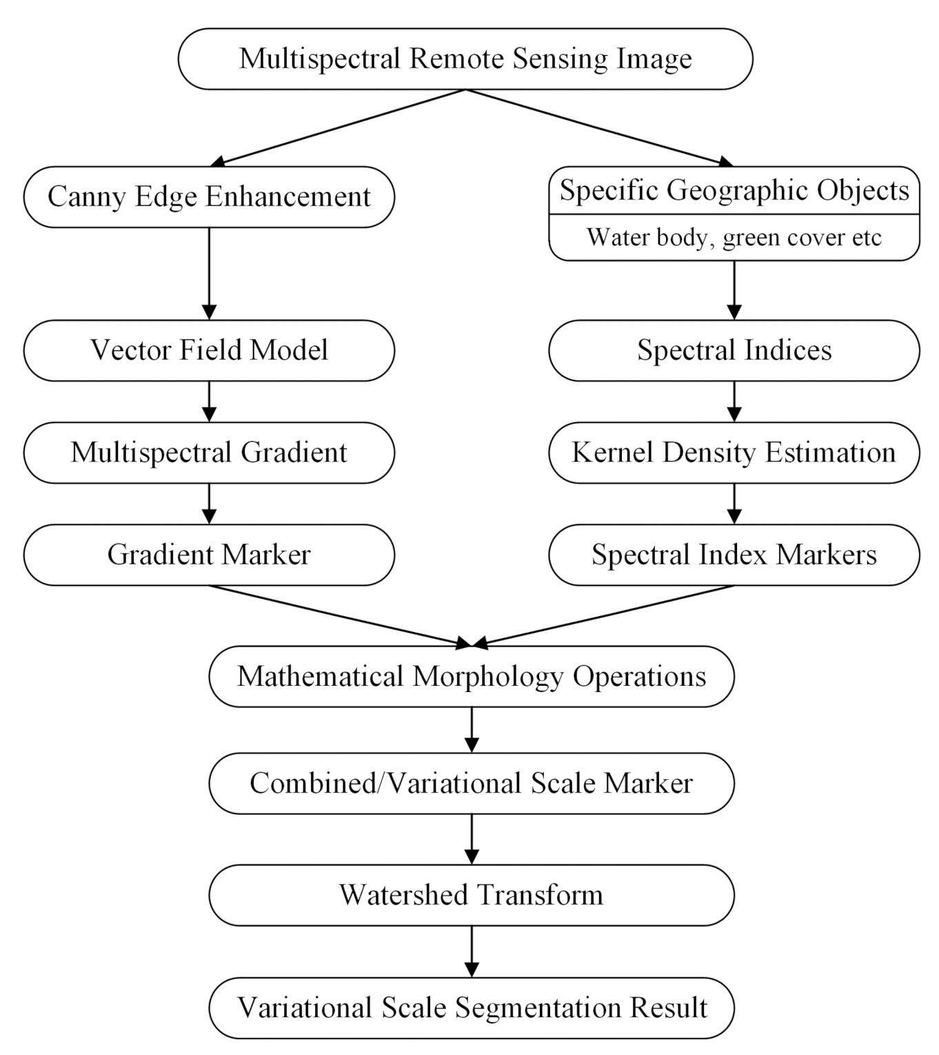
We used the gradient and spectral index markers for scale-variable watershed segmentation. The marker-controlled watershed transformation proceeds by using an automatic thresholding technique and a mathematical morphology method based on spectral indices and gradient images. Two marker images were generated from the gradient and spectral indices. The two marker images were then combined into one marker image for watershed transformation segmentation. Therefore, the key step in our method was to generate a marker image that integrates the gradient marker and spectral indices appropriately. The procedure for the proposed method is shown in Figure 2.
(1) Obtain multispectral edge strength from the fusion of panchromatic and multispectral bands using the Canny method and vector field model.
(2) Generate a marker image for the gradient by using the method proposed by Hill et al. [48], which is referred to as the Hill-marker method for convenience.
(3) Choose spectral indices based on land cover in the target remote-sensing image.
(4) Generate a marker image based on a histogram of spectral indices.
(5) Derive a final marker from the gradient and spectral index markers using intersection, erosion, thinning, and union operations from mathematical morphology.
(6) Perform marker-controlled watershed transformation segmentation.
3.2. Marker Generation from Multispectral Gradient using the Vector Field Model
The panchromatic and multispectral bands are fused to obtain a multispectral remote-sensing image with a higher spatial resolution. The first fundamental form based on the vector field model [49] is used to derive a multispectral gradient using the Canny method. Let be a multispectral image in the form of a vector field with bands and . The value of I at any given point is an n-dimensional vector. The gradient of in the ith band can be written as
and its squared norm (i.e., the first fundamental form) is
where the eigenvectors of the matrix can be used to obtain the directions of the maximal and minimal changes. Therefore, the eigenvalues of the matrix G can be represented by the gradient of the image, and the eigenvectors of G can be used to determine the edge direction. By using elementary algebra calculations, the maximum and minimum eigenvalues can be defined as follows:
The eigenvectors are , where the angles are given by
and
Sapiro and Ringach [49] suggested that the gradient of a multispectral remote-sensing image should not be represented by the maximal value among the eigenvalues but by how compares to . Therefore, the multispectral gradient can be defined as
After obtaining the gradient of a multi-spectral remote-sensing image, we applied the moving threshold method proposed by Hill et al. [48] to generate a marker image .
3.3. Marker Generation for Spectral Indices Based on a Histogram
Spectral indices, which are used to enhance the information of some ground objects, such as vegetation, soil, and water bodies, are correlated with specific ground objects. For example, NDVI [50] primarily enhances vegetation information, whereas NDWI [51,52,53] can be used to boost water-body information. There are also many other spectral indices, such as EVI [54], green NDVI [19], MSR [55], MTVI2 [56], TSAVI [57], MSAVI [58], ARVI [59], SARVI [59], OSAVI [60], and SR × NDVI [61], [52], [53], and shadow indices [62].
Here, we employed these spectral indices to generate a marker for the target objects in a remote-sensing image. To ensure that ground objects with complex internal textures can be segmented into a single region, it is important to apply a thresholding technique to obtain spectral index markers. Many unimodal thresholding techniques have been proposed in previous studies [63,64]. However, the goal of our study was not to retrieve accurate information associated with an object using spectral indices (e.g., water bodies can be segmented using the NDWI) but to obtain a marker image from spectral indices for watershed segmentation.
Here, we used kernel density estimation (KDE) to obtain a marker image. Most thresholding techniques are based on histograms. However, there are many local maxima and minima that can have a negative effect on determining a threshold. Unlike a histogram, KDE can represent the overall trend of the grayscale distribution in an image.
Given that is a random sample from a distribution F with density , the kernel density estimate of is given by
where is the kernel function. Because the probability density function of the spectral index commonly contains one or more peaks, we used the following Gaussian function as a kernel:
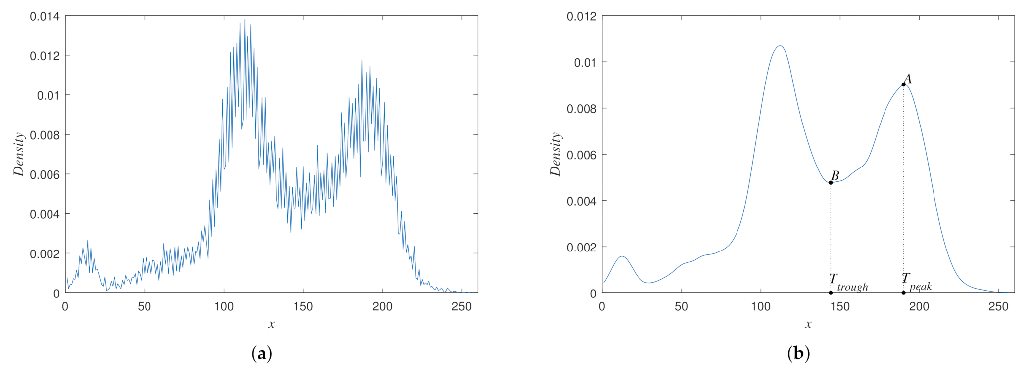
In Figure 3, we present an example to analyze the differences between the KDE and the histogram of an image. One can see that there are many local extrema in the histogram in Figure 3a. Therefore, we cannot easily identify useful local extrema, even though the trend of the curve can be visibly identified. In the KDE results in Figure 3b, the overall trend is clear and free of noise, so local extrema can be located correctly.
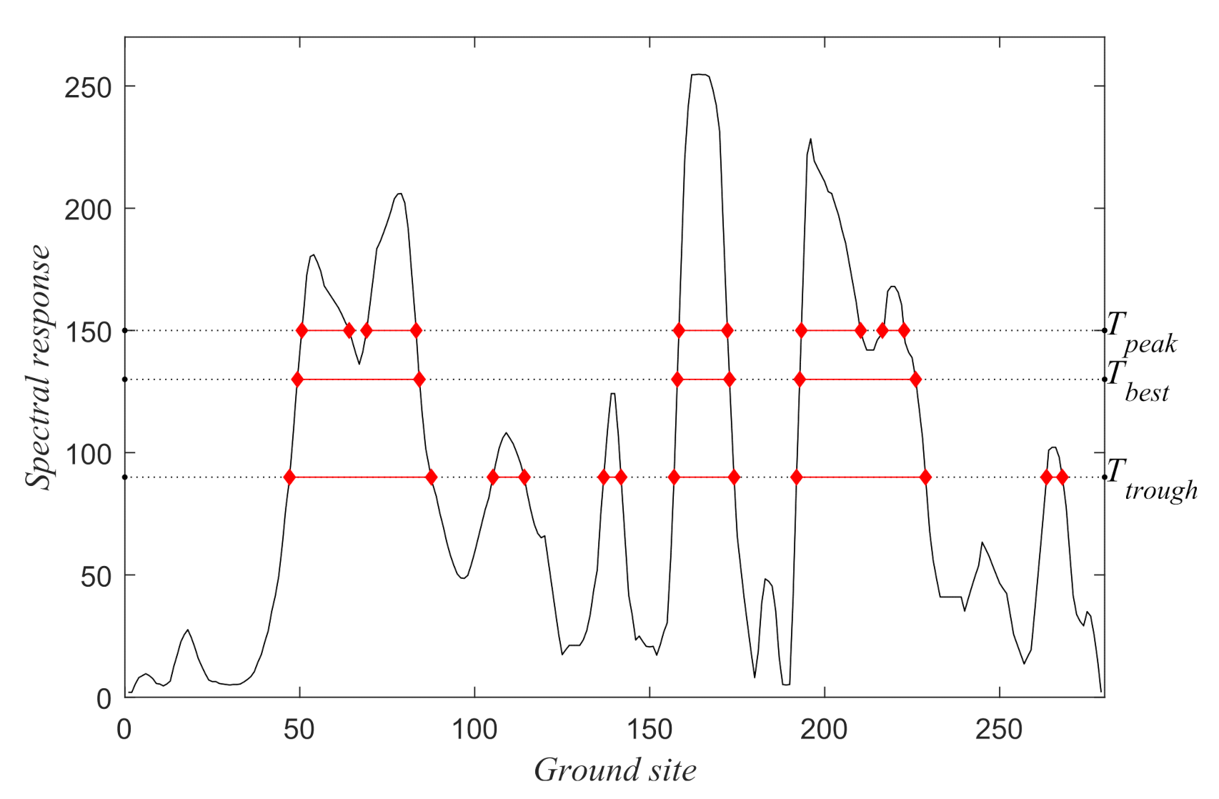
Because spectral indices are mainly used to enhance the information of the corresponding ground objects, a higher value indicates a higher probability of being the corresponding object. Additionally, the grayscale distribution of ground objects is typically normally distributed. Therefore, information on ground objects is relative to the last peak. To identify the last peak, we must find the accurate location of the peak (point A in Figure 3b) and the trough (point B in Figure 3b) on the left of the last peak. The peak A () and trough B () points can be obtained as
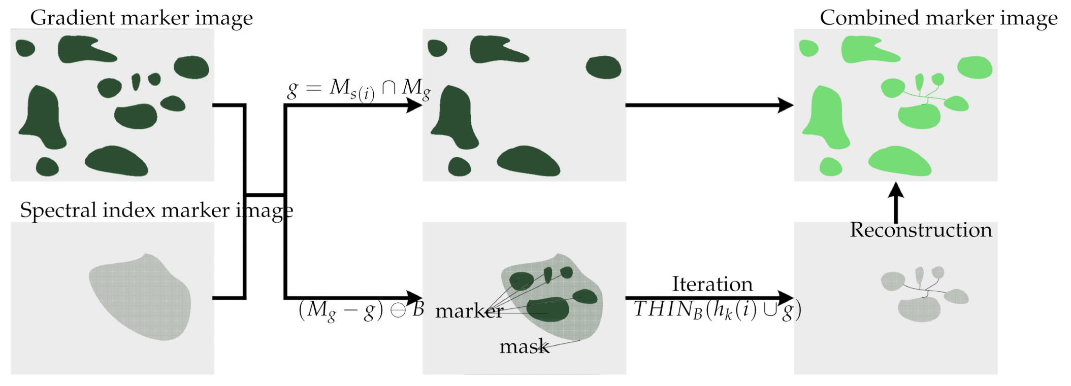
It is necessary to combine the markers from the gradient and spectral indices into a single marker image to perform watershed transformation segmentation efficiently. Two main factors should be considered when combining these markers. First, we must ensure that the spectral indices can be used to maintain the original scales of ground objects in the segmentation results. Second, the gradient information must be unaffected so that land cover can be segmented without the representation of specific spectral indices. Therefore, we must find a way to satisfy these two conditions. Here, mathematical morphology was used to reconstruct a marker image by combining the gradient and spectral indices.
Assume that and are marker images from the gradient and ith spectral index, respectively. The inflow for the combined marker-image-based spectral indices and gradient markers is presented in Figure 4.
and
where sign() is the signum function.
Then, the optimal threshold should be chosen from the interval .
3.4. Segmentation via Combination of Markers from Spectral Indices and Gradient Markers
First, we obtained the intersection of the gradient and spectral index marker images as follows:
Second, the gradient marker minus spectral index marker was defined as
where B is the structuring element.
We then used the intersection g as a marker and as a mask to reconstruct a new marker. Here, the reconstruction of from g, denoted as , was defined as
This reconstruction step was iterated to maintain the connectivity of the marker image while transforming the spectral index markers into one-pixel-wide lines.
Finally, the final Marker M was defined as
where n is the number of spectral indices based on the land cover distribution. The combined marker from the gradient and spectral index markers can be obtained using Algorithm 1.
| Algorithm 1 Generating a combined marker image based on spectral indices and gradient markers. |
| Input: Gradient marker image Number of spectral index marker images N The ith spectral index marker image Output: Combined marker image
|
Finally, the minima imposition technique [65] was employed for the watershed transformation based on the final marker image.
4. Experiments and Results
4.1. Performance Evaluation
, , and [66] were used to evaluate the performance of edge detection using different algorithms. and denote the source and target edge pixels, respectively. Matching was defined as true when the neighborhood of an edge pixel in includes the edge pixel in and there is no pixel between and . The neighborhood distance was set to three pixels in this study. and were defined as follows:
where is the number of edge pixels in matched with , is the number of edge pixels in matched with , and and are the numbers of edge pixels in and , respectively. According to Equations (23) and (24), the , which is the weighted harmonic mean of and , is defined as
where is a given parameter.
4.2. Influence of the Threshold for Spectral Indices on Segmentation
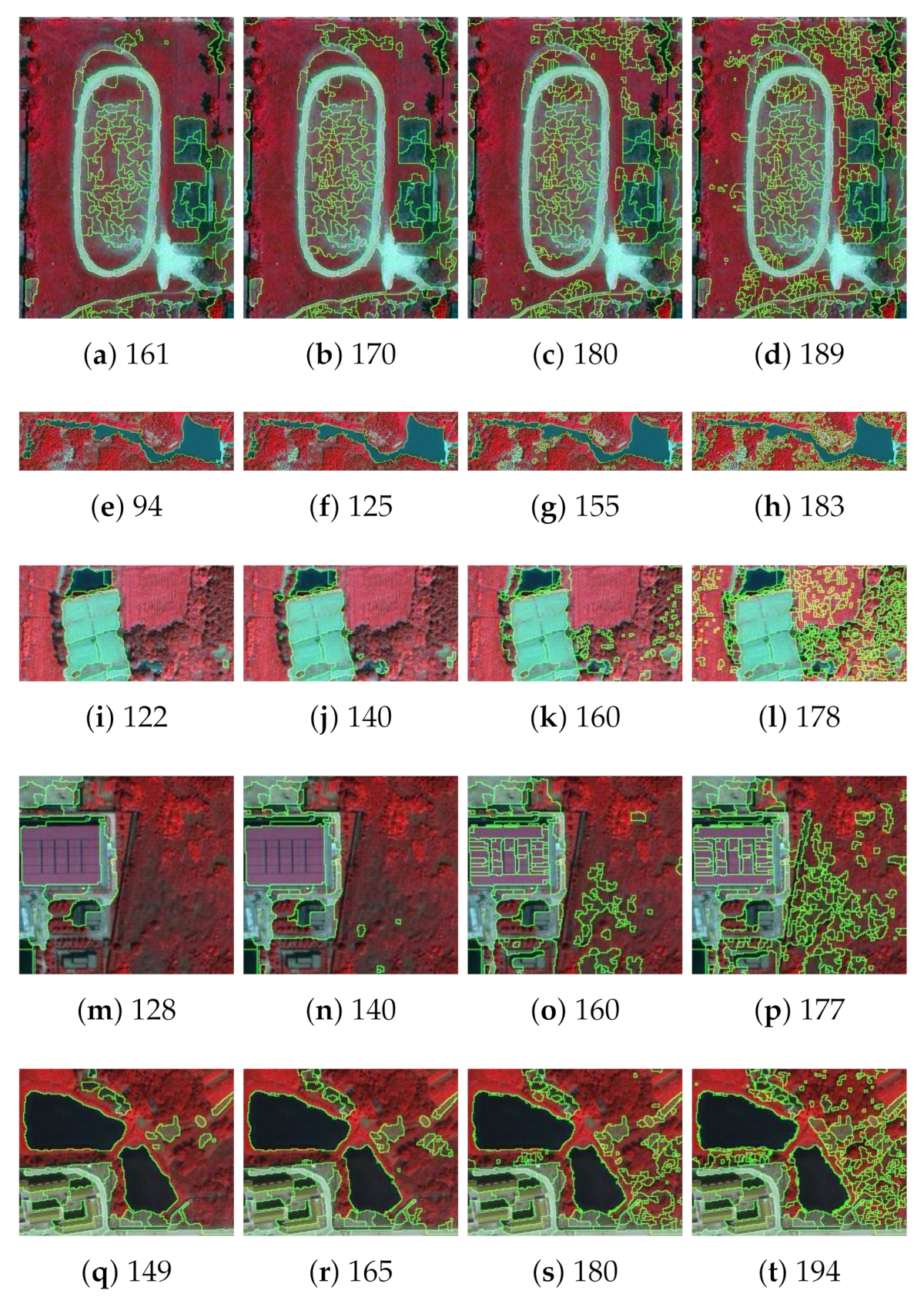
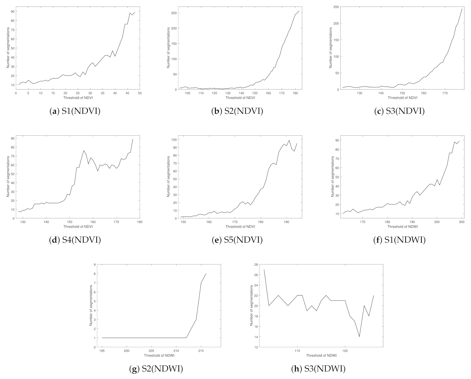
The five subsets from images D1 and D2 shown in Figure 5 were used to analyze the influence of the threshold for spectral indices on image segmentation. Excluding the parameter of in the Hill-marker method [48], when obtaining a marker image of a gradient, the range is the only parameter for the proposed method. The influence of this parameter on the segmentation results of the subsets was evaluated with the goal of determining an optimal setting. The ranges of the spectral indices of the images calculated using Equations (9) and (10) are listed in Table 1.
To illustrate the influence of the threshold parameter of the spectral index for marker generation, given the parameter value of , segmentation results for four different threshold values applied to generate spectral index markers based on NDVI and NDWI are presented in Figure 6 and Figure 7, respectively. Additionally, Figure 8 presents watershed segmentation results for the Hill-marker method, where the parameter of was also set to 10, to demonstrate the superiority of the proposed method.
First, as shown in Figure 6 for NDVI, the segmentation results for vegetable cover tend to contain more segments as the threshold value increases for all five subset images. Regardless, compared to the Hill-marker watershed segmentation results in Figure 8, one can see that green objects identified by the proposed method with the NDVI marker were segmented better than those identified by the Hill-marker method, particularly when the threshold value of the spectral index was close to . Consider the segmentation results of S1, S2, and S4 as examples for further analysis. One can see that the segmentation results for green cover in Figure 8a,b,d contain large numbers of fragments that are adjacent and that all belong to the green cover. This phenomenon was less apparent when using the proposed method.
Second, the shadows of ground objects generally have negative effects on segmentation and were segmented into a different region in Figure 8c. In contrast, in Figure 6, the green cover and its shadows were segmented into the same region. The shadows of the green objects are highlighted with white circles. Additionally, various adjacent vegetative covers can be segmented into the same region. For example, the green cover in image S3 consists of both shrubs and forest trees. In the segmentation results of the Hill-marker method, there are boundaries between these different types of plants. In contrast, they are segmented into the same region in Figure 6i,j when using the proposed method.
Regarding the segmentation based on the NDWI marker image in Figure 7, one can see similar results compared to the NDVI marker image. When the threshold value increases, the number of segmentation regions tends to increase. However, unlike the comparison between the segmentation results in Figure 7 and Figure 8, the proposed method based on NDWI markers alone is not superior to the Hill-marker method. The result for image S5 is inferior to that generated by the Hill-marker method because the water pool on the right cannot be segmented accurately, and its boundary is visibly separated from the real boundary. This is because the internal spectral response difference for the water cover region is high. Therefore, if there is more than one region of water in an experimental image with multiple peaks corresponding to multiple water cover types, the threshold of NDWI for marker generation is difficult to determine.
4.3. Automatic Selection of Optimal Segmentation Regions
As shown in Figure 6 and Figure 7, the selection of a threshold for the spectral indices has a distinct influence on the final segmentation results. It is necessary to select parameters to obtain optimal segmentation results automatically, where segmentation can accurately reflect the scales of ground objects in remote-sensing images. For watershed transformation segmentation, more markers generate more segments. Therefore, the threshold for the spectral index , which determines the number of markers generated from the spectral index, is key to the performance of segmentation.
When the threshold is , the number of segments may increase when uncorrelated ground objects are segmented. This is because correctly joined ground objects may be divided into several disjointed regions with different internal textures. When the threshold is , the number of segments may also increase. As shown in Figure 9, we simulated a one-dimensional spectral response to explain this phenomenon. One can see that the segment number may decrease and then increase as the threshold increases from to . Therefore, we must identify the most suitable threshold for generating marker images.
Figure 10 presents the numbers of segmentation regions when the threshold was selected from the range of for the subset images. Figure 10a–e are based on using the NDVI for S1 to S5, respectively. Figure 10f–h are based on using the NDWI marker for S2, S3, and S5, respectively. One can see that most of the curves generally tend to increase. However, once can also see trends of small decreases (Figure 10b,d,h), fluctuations (Figure 10a,c,f), or unchanged values (Figure 10e,g). When the curve visibly increases, it indicates that the green or water covers tend to be segmented into more fragments. Therefore, we must identify the minimum number of segmentations to guarantee that there are no (or few) adjacent segmented regions of green or water covers in the results.
When is obtained based on spectral indices from remote-sensing data, spectral markers can be obtained in Algorithm 2:
| Algorithm 2 Obtaining the optimal thresholds of spectral indices for generating marker images. |
| Input: Multispectral band image T Output: Spectral index marker image
|
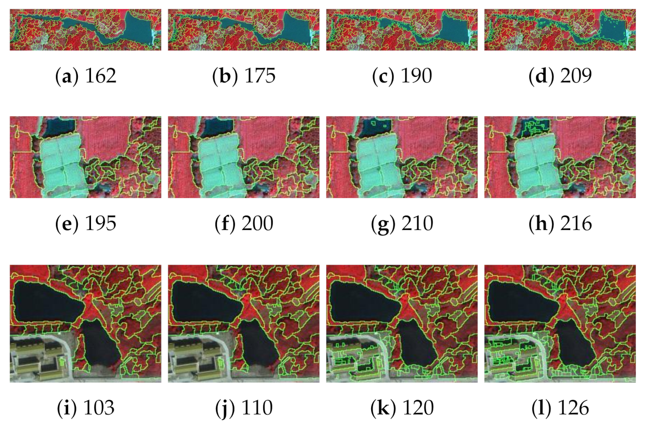
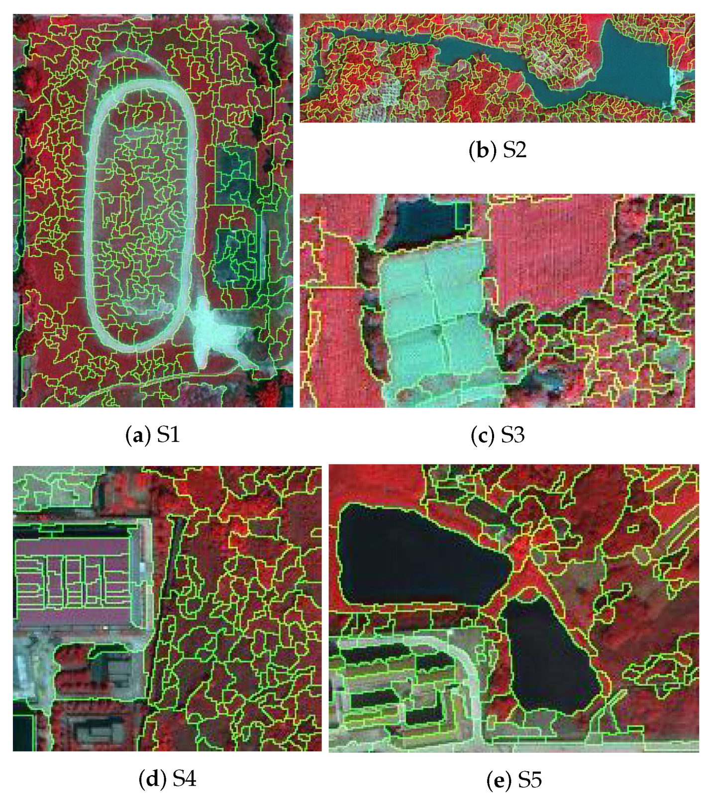
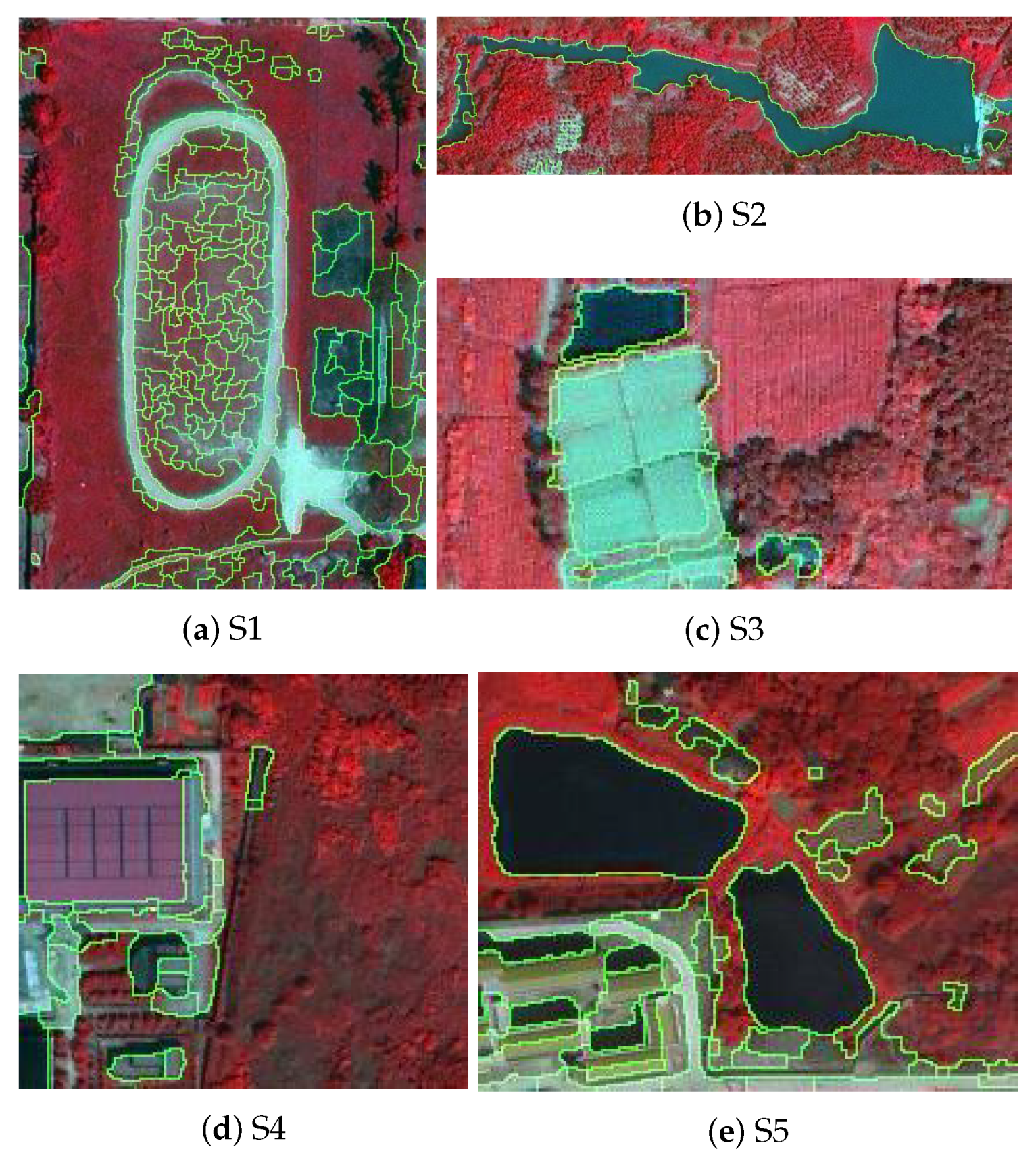
Figure 11 presents the optimal segmentations for the five subsets of data, as well as expressive segmentation results. First, the green covers in all subsets were segmented into one region. Land covers with different scales, such as buildings and green covers, can be segmented into different regions. For example, there is a significant difference in the scale of buildup in S1, S4, and S5. However, these buildups can be segmented with little influence from the parameter of the spectral index threshold. Additionally, the water bodies in the images were also segmented accurately. Therefore, the proposed method for automatically selecting the threshold for spectral indices can obtain expressive segmentation results.
4.4. Influence of the Scale Parameter
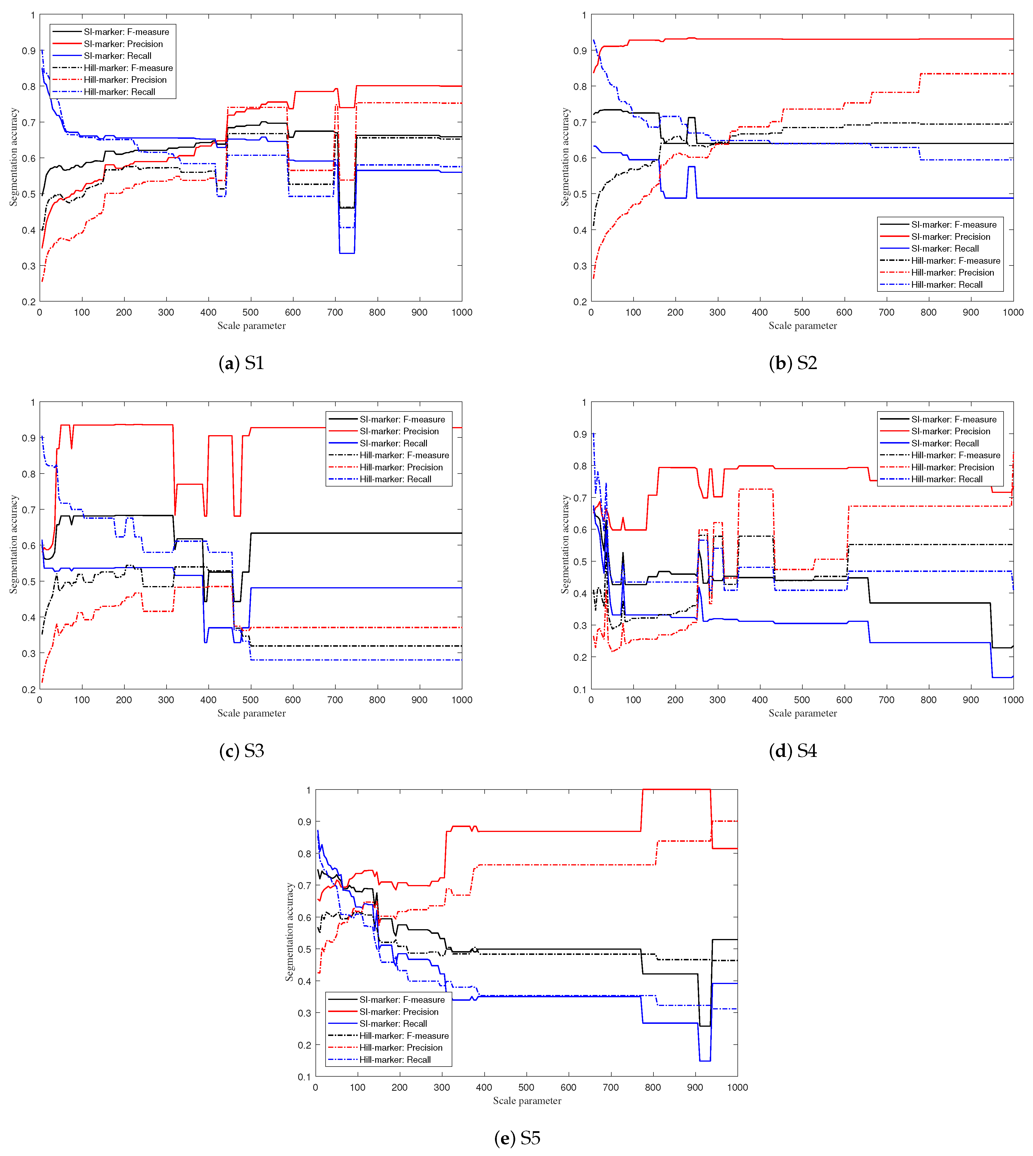
Based on the automatic selection of the threshold parameter, the segmentation results for different scale parameters are presented in Figure 12 to analyze the influence of the this parameter comparatively. Here, the scale parameter (scale) of the watershed transformation was defined within the interval of [5, 1000] in increments of five. We can see that all the curves of using the SI-marker are superior to those using the Hill-marker. In the following section, we present our analysis in detail.
In Figure 12a, the values of first increase and then slightly decrease as the scale parameter increases. The highest reaches its maximum value when the scale parameters are 525, 530, and 535. The reason for the values of being low in the beginning is that there were still some fragments of green cover in the segmentation results.
For dataset S2, the best performance () was achieved when the scale parameter was relatively small at 90. The SI-marker method is distinctly superior to the Hill-marker method.
In Figure 12c, the curve of using the SI-marker method was significantly higher than that using the Hill-marker method. The main reason for this result is that the of the SI-marker method is much higher than that of the Hill-marker method. This means that the boundaries of the segments have high congruency with the real boundaries between ground objects. The highest appeared in the range of , which is relatively low.
As shown in Figure 12d, the curve of using the SI-marker method was not higher than that using the Hill-marker method for all scale parameters. The SI-marker method can achieve the best performance () when the scale parameter is five. However, as long as the scale parameter is less than 250, the SI-marker method is superior to the Hill-marker method.
Figure 12e reveals that the SI-marker method is generally superior to the Hill-marker method. The best performance when using the SI-marker method occurs when the scale parameter is five. The main advantage of the SI-marker method is that the accuracy of the boundaries detected by the SI-marker method is higher than that detected by the Hill-marker method.
By comparing the five curves, one can conclude that the performance of the SI-marker method is visibly and consistently superior to that of the Hill-marker method when the scale is small. Additionally, the of the SI-marker method was always higher than that of the Hill-marker method, which indicates that there were more accurate segmentation boundaries. Furthermore, there were many fragments in the segmentation results, so the for some datasets when using the Hill-marker method was higher than that when using the SI-marker method, particularly when the scale parameter was small for S2 and S4.
To analyze the optimal scale parameter for our proposed method further, local variance was used as a tool to explore the optimal scale. Given an image I, the local variance can be defined as
where is the local mean of the image. Given that is a weighted neighborhood centered on a pixel, the local variance can be rewritten as
with
The mean of the local variance was estimated as
where M and N represent the size of the image
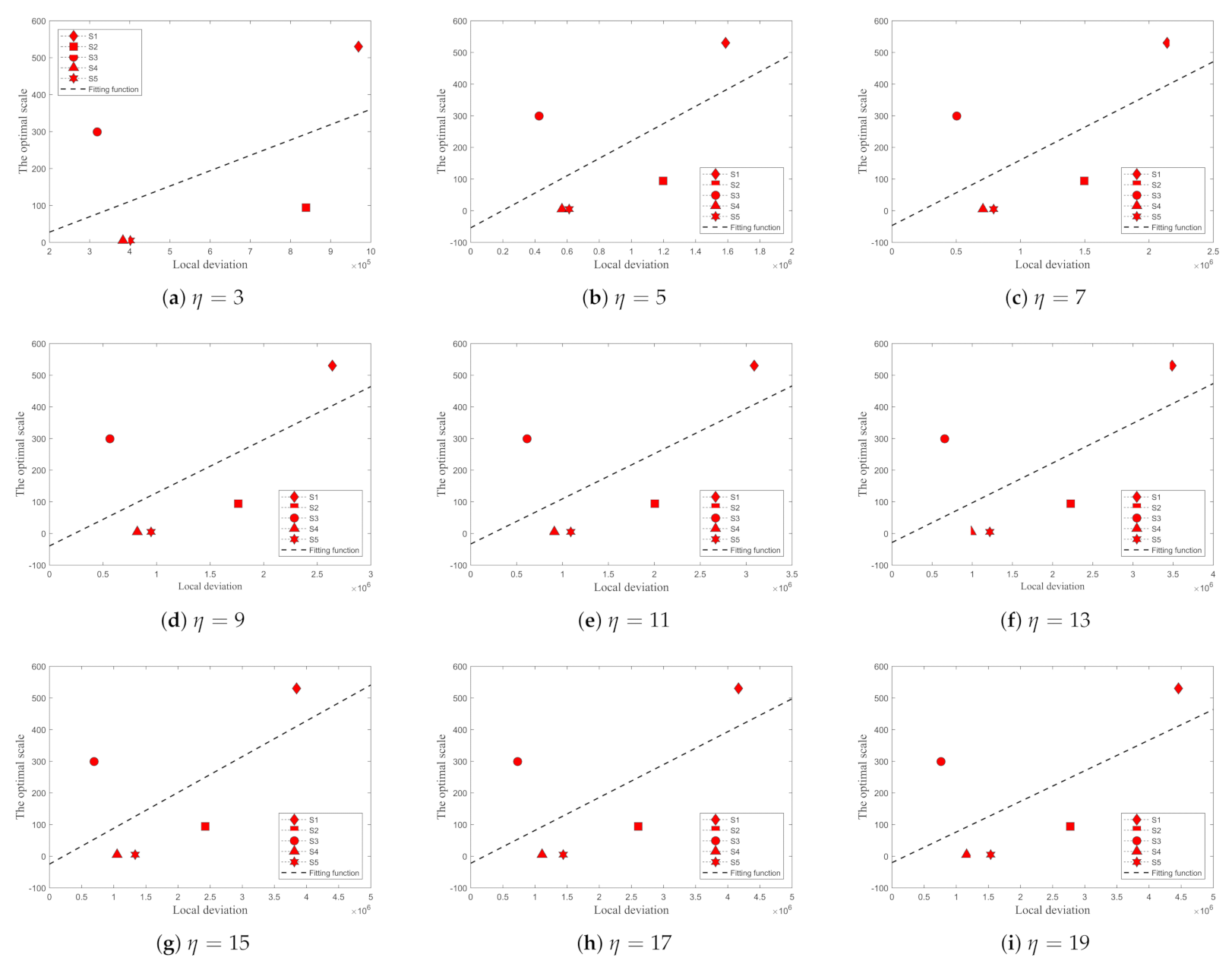
We used the to analyze the relationship between the local variance and the optimal scale parameter. Figure 13 plots the relationship between the scale and the corresponding local variance of regions marked by NDVI for each subset image to reflect the influence of local variance. Green objects, which represent a high proportion of land cover in the datasets, are important for evaluating the performance of segmentation. The weighted neighborhood size was drawn from the interval of [3, 19] with a step size of two. Additionally, the curves of the fitting function represent the fitting results for the point sets of {S1, S2, S3, S4, and S5}.
First, one can see that the relationship between the optimal scale and the local variance was stable. The relative positions of the five datasets in Figure 13 remained almost unchanged, even though the size of the neighborhood window was different for each subfigure. Second, one can see that the optimal scale for these datasets increases with increasing local variance, except for S3. For S3, the segmentation accuracy remained high when the scale parameter was low, even though the optimal scale and corresponding local variance do not match the first-order fitting curve.
4.5. Comparision
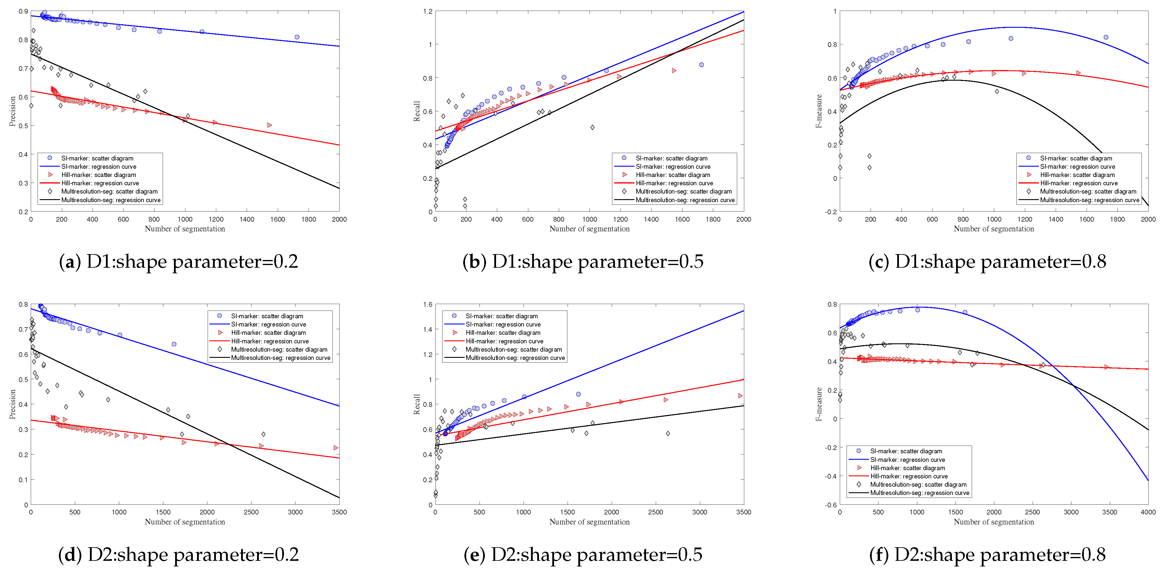
To highlight the effectiveness of the proposed method, datasets D1 and D2, where there was large-scale green cover and some water bodies, were used as experimental datasets for comparative segmentation analysis. In this segmentation experiment, the proposed method was compared to the Hill-marker watershed segmentation and the multiresolution segmentation method (MRS) [17] embedded in the eCognition Developer software. The scale parameters for the SI-marker and the Hill-marker watershed segmentation methods were selected from the interval [10, 500] with a step size of 10. For the MRS segmentation method, the scale parameter was selected from and the range of [100, 1000] with a step size of 10. The shape parameter was selected from , and the compact parameter was set to the default value of 0.5. Figure 14 presents the curves of , , and with different numbers of segmentation regions using different methods.
First, decreased as the number of segmentation regions increased for all methods. However, the of the proposed method based on the SI-marker was superior to that of the other methods. The curve in Figure 14b reveals that the Hill-marker watershed segmentation method performed better than the SI-marker watershed segmentation method when the number of segmentation regions was small. When the number of segmentation regions was greater than 500, the of the proposed method was visibly higher than that of the other methods, particularly when the of the Hill-marker method decreased sharply. Third, regarding the values of all methods, the proposed method exhibited the best performance for different numbers of segmentation regions. Additionally, the of SI-marker watershed segmentation increased and then decreased with the number of segmentation regions with a maximum value near 0.8.
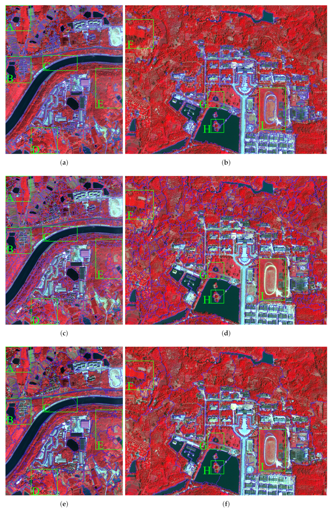
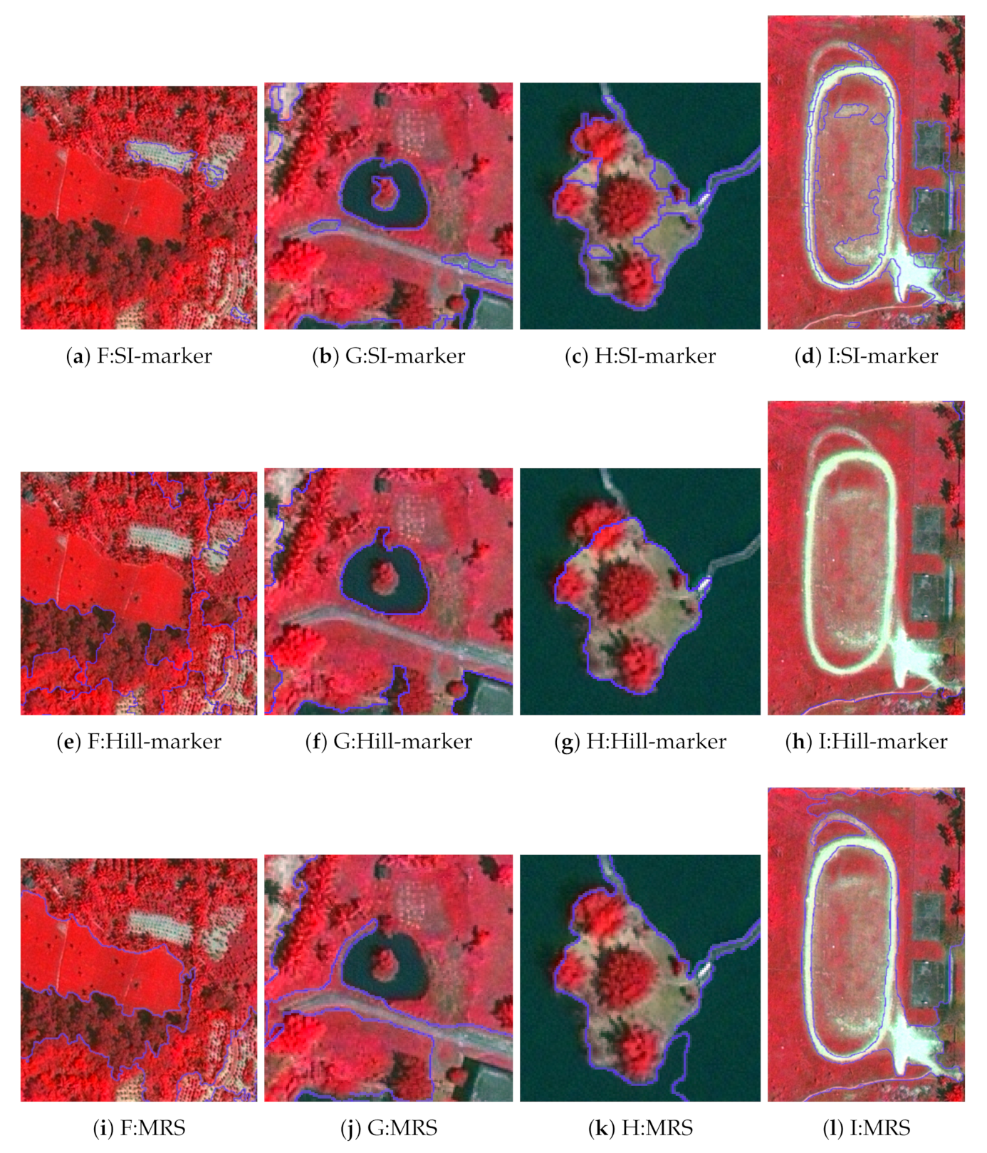
Figure 15 presents the best segmentation results for the SI-marker, and Hill-marker, and MRS methods on datasets D1 and D2. Segmentation by the SI-marker watershed transformation clearly provided better results than the other methods. In particular, the green objects identified by the SI-marker watershed transformation were mostly segmented into one region, even though the spectral information of the green objects was not consistent. In the segmentation results of the Hill-marker watershed method, there was significant over-segmentation. The MRS method also yielded some over-segmentation. Regarding the segmentation results for water body cover, the SI-marker watershed method was superior to the MRS method. To illustrate the effectiveness of the SI-marker watershed method, we selected nine regions for further analysis.
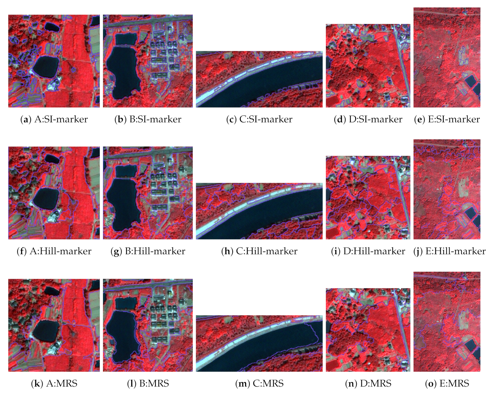
To illustrate the details of segmentation clearly, Figure 16 and Figure 17 present the segmentation results for regions A, B, C, D, E, F, G, and I using the three methods. First, in regions A, B, D, E, and F, where the spectral information of green objects contained visible inconsistency, the SI-marker watershed transformation method obtained a single region, whereas the Hill-marker watershed transformation and MRS methods separated each region into several segments. Second, because the scales of the best segmentation results for the Hill-marker watershed transformation and MRS methods were large, many small-scale objects were ignored and incorrectly segmented into other ground objects. However, an object with a small scale can be identified using the proposed method. For example, the bare area in region F, small-scale green objects in regions G and H, two buildings in region I, and many buildings in regions A and B were maintained as one segment. Third, in addition to green objects, water bodies can also be incorrectly segmented. For example, the water bodies were missed in the segmentation results for regions A, B, C, E, and G for the Hill-marker watershed transformation and MRS methods. In contrast, the SI-marker watershed method guaranteed that green and water objects were segmented properly and that objects of different scales can maintain good segmentation performance.
5. Conclusions
In this study, we proposed a novel variational-scale multispectral image-segmentation method using spectral indices. Because geographical objects on the Earth’s surface have different scales, remote-sensing images should be segmented according to the different scales of ground objects. We found that the spectral indices that are primarily used to enhance the information of ground objects can ignore the scale problem of geographical objects. Therefore, we introduced spectral indices into marker generation for marker-controlled watershed transformation segmentation. Spectral indices were used to generate markers for watershed segmentation based on KDE. Next, a gradient based on the Canny method and VFM was used to generate markers using Hill’s method [48]. Reconstruction based on mathematical morphology was then used to combine the gradient and spectral index markers. Additionally, the automatic selection of a spectral index threshold was proposed for optimal variational-scale watershed segmentation based on mathematical morphology.
Two multispectral high-resolution remote-sensing images were used to validate the proposed remote-sensing image-segmentation method. In an image segmentation experiment, we compared our method to the multi-scale watershed transformation method proposed in [48] and the MRS method embedded in the eCognition Developer software. The , , and measures proposed in [66] were used to evaluate the segmentation results. Additionally, we analyzed the influence of the scale parameter on image segmentation based on seven subsets of remote-sensing images from datasets D1 and D2. The results revealed that the proposed method provides improved performance compared to the Hill-marker watershed transformation and MRS methods. We can draw the following conclusions:
(1) The revealed that the proposed method produces more accurate segmentation results compared to the watershed transformation method from [48] and the MRS [17] method for varying numbers of segments.
(2) The proposed segmentation method can visually and consistently maintain the original scales of ground objects in image-segmentation results at different segmentation scales, particularly for green land cover.
(3) Our method provides more robust image segmentation under different and scale values when the geographical objects in remote-sensing images can be enhanced by spectral indices.
Author Contributions
K.W. had the original idea for the study and drafted the manuscript. K.W. and H.C. contributed to perform the experimentation. L.C. and J.X. contributed data curation. All authors contributed to writing and polishing of the manuscript. All authors have read and agreed to the published version of the manuscript.
Funding
This research was funded by the National Natural Science Foundation of China (Grant No. 41771358), the Natural Science Foundation of Jiangsu Province, China (Grant No. BK20140842), the Fundamental Research Funds for the Central Universities: B210202011, and Guangdong water conservancy science and technology innovation project: 2020-04.
Institutional Review Board Statement
Not applicable.
Informed Consent Statement
Not applicable.
Data Availability Statement
Not applicable.
Acknowledgments
The authors would like to acknowledge the constructive criticism of anonymous reviewers.
Conflicts of Interest
The authors declare there is no conflict of interest regarding the publication of this study.
References
- Blaschke, T.; Hay, G.J. Object-oriented image analysis and scale-space: Theory and methods for modeling and evaluating multi-scale landscape structure. Int. Arch. Photogramm. Remote Sens. 1998, 34, 22–29. [Google Scholar]
- Blaschke, T.; Strobl, J.; Zeil, P. Object-oriented image processing in an integrated gis/remote sensing environment and perspectives for environmental applications. In Environmental Information for Planning, Politics and the Public; Cremers, A., Greve, K., Eds.; Metropolis: Marburg, Germany, 2000. [Google Scholar]
- Schiewe, J.; Tufte, L.; Ehlers, M. Potential and problems of multi-scale segmentation methods in remote sensing. GeoBIT/GIS 2001, 54, 34–39. [Google Scholar]
- Speake, T.; Mersereau, R.M. Segmentation of high-resolution remotely sensed data concepts, applications and problems. Jt. ISPRS Comm. Symp. Geospat. Theory Proc. Appl. 2002, 34, 380–385. [Google Scholar]
- Schiefer, F.; Kattenborn, T.; Frick, A.; Frey, J.; Schall, P.; Koch, B.; Schmidtlein, S. Mapping forest tree species in high resolution UAV-based RGB-imagery by means of convolutional neural networks. ISPRS J. Photogramm. Remote Sens. 2020, 170, 205–21539. [Google Scholar] [CrossRef]
- Nezami, S.; Khoramshahi, E.; Nevalainen, O.; Pölönen, I.; Honkavaara, E. Tree species classification of drone hyperspectral and rgb imagery with deep learning convolutional neural networks. Remote Sens. 2020, 12, 1070. [Google Scholar] [CrossRef] [Green Version]
- Grinias, I.; Panagiotakis, C.; Tziritas, G. MRF-based Segmentation and Unsupervised Classification for Building and Road Detection in Peri-urban Areas of High-resolution. ISPRS J. Photogramm. Remote Sens. 2016, 122, 145–166. [Google Scholar] [CrossRef]
- Marçal, A.R.S.; Borges, J.S.; Gomes, J.A.; Pinto da Costa, J.F. Land cover update by supervised classification of segmented aster images. Int. J. Remote Sens. 2005, 26, 1347–1362. [Google Scholar] [CrossRef]
- Chen, Y.; Wang, J.; Li, X. Object-oriented classification for urban land cover mapping with aster imagery. Int. J. Remote Sens. 2007, 28, 4645–4651. [Google Scholar] [CrossRef]
- Duveiller, G.; Defourny, P.; Desclée, B.; Mayaux, P. Deforestation in central africa: Estimates at regional, national and landscape levels by advanced processing of systematically-distributed landsat extracts. Remote Sens. Environ. 2008, 112, 1969–1981. [Google Scholar] [CrossRef]
- Myint, S.W.; Yuan, M.; Cerveny, R.S.; Giri, C.P. Comparison of remote sensing image processing techniques to identify tornado damage areas from landsat tm data. Sensors 2008, 8, 1128–1156. [Google Scholar] [CrossRef] [Green Version]
- Jobin, B.; Labrecque, S.; Grenier, M.; Falardeau, G. Object-based classification as an alternative approach to the traditional pixel-based classification to identify potential habitat of the grasshopper sparrow. Environ. Manag. 2008, 41, 20–31. [Google Scholar] [CrossRef]
- Cufí, X.; Muñoz, X.; Freixenet, J.; Martí, J. A review of image segmentation techniques integrating region and boundary information. Adv. Imaging Electron Phys. 2003, 120, 1–39. [Google Scholar]
- Moghaddamzadeh, A.; Bourbakis, N. A fuzzy region growing approach for segmentation of color images. Pattern Recognit. 1997, 30, 867–881. [Google Scholar] [CrossRef]
- Xiao, P.; Feng, X.; An, R.; Zhao, S. Segmentation of multispectral high-resolution satellite imagery using log gabor filters. Int. J. Remote Sens. 2010, 31, 1427–1439. [Google Scholar] [CrossRef]
- Karantzalos, K.; Argialas, D. Improving edge detection and watershed segmentation with anisotropic diffusion and morphological levellings. Int. J. Remote Sens. 2006, 27, 5427–5434. [Google Scholar] [CrossRef]
- Baatz, M.; Schäpe, A. Multiresolution segmentation—An optimization approach for high quality multi-scale image segmentation. In Angewandte Geographische Informationsverarbeitung XII, Beiträge zum AGIT-Symposium Salzburg; Blaschke, T., Strobl, J., Greisebener, G., Eds.; Wichmann: Heidelberg, Germany, 2000. [Google Scholar]
- Evans, C.; Jones, R.; Svalbe, I.; Berman, M. Segmenting multispectral landsat tm images into field units. IEEE Trans. Geosci. Remote Sens. 2002, 40, 1054–1064. [Google Scholar] [CrossRef]
- Gitelson, A.A.; Kaufman, Y.J.; Merzlyak, M.N. Use of a green channel in remote sensing of global vegetation from eos-modis. Remote Sens. Environ. 1996, 58, 289–298. [Google Scholar] [CrossRef]
- Li, Y.; Gong, P. An efficient texture image segmentation algorithm based on the gmrf model for classification of remotely sensed imagery. Int. J. Remote Sens. 2005, 26, 5149–5159. [Google Scholar] [CrossRef]
- Sarkar, A.; Biswas, M.K.; Kartikeyan, B.; Kumar, V.; Majumder, K.L.; Pal, D.K. A mrf model-based segmentation approach to classification for multispectral imagery. IEEE Trans. Geosci. Remote Sens. 2002, 40, 1102–1113. [Google Scholar] [CrossRef]
- Lizarazo, I.; Elsner, P. Fuzzy segmentation for object-based image classification. Int. J. Remote Sens. 2009, 30, 1643–1649. [Google Scholar] [CrossRef]
- Marr, D. Early processing of visual information. Phil. Trans. R. Soc. Lond. B 1976, 275, 483–524. [Google Scholar]
- Marr, D. Analyzing natural images: A computational theory of texture vision. Cold Spring Harbor Symp. Quant. Biol. 1976, 40, 647–662. [Google Scholar] [CrossRef]
- Zhang, X.; Xiao, P.; Feng, X. Object-specific optimization of hierarchical multiscale segmentations for high-spatial resolution remote sensing images. ISPRS J. Photogramm. Remote Sens. 2020, 159, 308–321. [Google Scholar] [CrossRef]
- Benz, U.C.; Hofmann, P.; Willhauck, G.; Lingenfelder, I.; Heynen, M. Object-oriented fuzzy analysis of remote sensing data for gis-ready information. ISPRS J. Photogramm. Remote Sens. 2004, 58, 239–258. [Google Scholar] [CrossRef]
- Ma, L.; Li, M.; Ma, X.; Cheng, L.; Du, P.; Liu, Y. A review of supervised object-based land-cover image classification. ISPRS J. Photogramm. Remote Sens. 2017, 130, 277–293. [Google Scholar] [CrossRef]
- Zhang, H.; Fritts, J.E.; Goldman, S.A. Image segmentation evaluation: A survey of unsupervised methods. Comput. Vis. Image Underst. 2008, 110, 260–280. [Google Scholar] [CrossRef] [Green Version]
- Chen, G.; Weng, Q.; Hay, G.J.; He, Y. Geographic object-based image analysis (geobia): Emerging trends and future opportunities. Gisci. Remote Sens. 2018, 55, 159–182. [Google Scholar] [CrossRef]
- Chen, G.; Ming, D.; Zhao, L.; Lv, B.; Zhou, K.; Qing, Y. Review on high spatial resolution remote sensing image segmentation evaluation. Photogramm. Eng. Remote Sens. 2018, 84, 629–646. [Google Scholar] [CrossRef]
- Espindola, G.M.; Camara, G.; Reis, I.A.; Monteiro, L.S.B.M. Parameter selection for region-growing image segmentation algorithms using spatial autocorrelation. Int. J. Remote Sens. 2006, 27, 3035–3040. [Google Scholar] [CrossRef]
- Corcoran, P.; Winstanley, A.; Mooney, P. Segmentation performance evaluation for object-based remotely sensed image analysis. Int. J. Remote Sens. 2010, 31, 617–645. [Google Scholar] [CrossRef]
- Johnson, B.; Xie, Z. Unsupervised image segmentation evaluation and refinement using a multi-scale approach. ISPRS J. Photogramm. Remote Sens. 2011, 66, 473–483. [Google Scholar] [CrossRef]
- Ming, D.; Li, J.; Wang, J.; Zhang, M. Scale parameter selection by spatial statistics for geobia: Using mean-shift based multi-scale segmentation as an example. ISPRS J. Photogramm. Remote Sens. 2015, 106, 28–41. [Google Scholar] [CrossRef]
- Wang, Y.; Qi, Q.; Liu, Y.; Jiang, L.; Wang, J. Unsupervised segmentation parameter selection using the local spatial statistics for remote sensing image segmentation. Int. J. Appl. Earth Obs. GeoInf. 2011, 32, 2015–2024. [Google Scholar] [CrossRef]
- Dragut, L.; Tiede, D.; Levick, S.R. Esp: A tool to estimate scale parameter for multiresolution image segmentation of remotely sensed data. Int. J. Geogr. Inf. Sci. 2010, 24, 859–871. [Google Scholar] [CrossRef]
- Dragut, L.; Csillik, O.; Eisank, C.; Tiede, D. Automated parameterisation for multiscale image segmentation on multiple layers. ISPRS J. Photogramm. Remote Sens. 2014, 88, 119–127. [Google Scholar] [CrossRef] [PubMed] [Green Version]
- Yang, J.; Li, P.; He, Y. A multi-band approach to unsupervised scale parameter selection for multi-scale image segmentation. ISPRS J. Photogramm. Remote Sens. 2014, 94, 13–24. [Google Scholar] [CrossRef]
- Zhang, X.; Du, S. Learning selfhood scales for urban land cover mapping with veryhigh-resolution satellite images. Remote Sens. Environ. 2016, 178, 172–190. [Google Scholar] [CrossRef]
- Yang, J.; He, Y.; Caspersen, J. Region merging using local spectral angle thresholds: A more accurate method for hybrid segmentation of remote sensing images. Remote Sens. Environ. 2017, 190, 137–148. [Google Scholar] [CrossRef]
- Dekavalla, M.; Argialas, D. A region merging segmentation with local scale parameters: Applications to spectral and elevation data. Remote Sens. 2018, 10, 2024. [Google Scholar] [CrossRef] [Green Version]
- Xiao, P.; Zhang, X.; Zhang, H.; Hu, R.; Feng, X. Multiscale optimized segmentation of urban green cover in high resolution remote sensing image. Remote Sens. 2018, 10, 1813. [Google Scholar] [CrossRef] [Green Version]
- Su, T. Scale-variable region-merging for high resolution remote sensing image segmentation. ISPRS J. Photogramm. Remote Sens. 2019, 147, 319–334. [Google Scholar] [CrossRef]
- Kavzoglu, T.; Erdemir, M.Y.; Tonbul, H. Classification of semiurban landscapes from very high-resolution satellite images using a regionalized multiscale segmentation approach. J. Appl. Remote Sens. 2017, 11, 035016. [Google Scholar] [CrossRef]
- Georganos, S.; Grippa, T.; Lennert, M.; Vanhuysse, S.; Johnson, B.A.; Wolff, E. Scale matters: Spatially partitioned unsupervised segmentation parameter optimization for large and heterogeneous satellite images. Remote Sens. 2018, 10, 1440. [Google Scholar] [CrossRef] [Green Version]
- Vincent, L.; Soille, P. Watershed in digital spaces: An efficient algorithm based on immersion simulations. IEEE Trans. Pattern Anal. Mach. Intell. 1991, 13, 583–598. [Google Scholar] [CrossRef] [Green Version]
- Beucher, S.; Meyer, F. The morphological approach to segmentation: The watershed transformation. In Mathematical Morphology and its Applications to Image Processing; Dougherty, E.R., Ed.; Marcel Dekker: New York, NY, USA, 1993. [Google Scholar]
- Hill, P.R.; Canagarajah, C.N.; Bull, D.R. Image segmentation using a texture gradient based watershed transform. IEEE Trans. Image Process. 2003, 12, 1618–1633. [Google Scholar] [CrossRef]
- Sapiro, G.; Ringach, D.L. Anisotropic diffusion of multivalued images with applications to color filtering. IEEE Trans. Image Process. 1996, 5, 1582–1586. [Google Scholar] [CrossRef] [PubMed]
- Roberts, L.G. Monitoring the vernal advancements and retrogradation (greenwave effect) of nature vegetation. In NASA/GSFC Final Report; NASA: Greenbelt, Philippines, 1974. [Google Scholar]
- Work, E.A.; Gilmer, D.S. Utilization of satellite data for inventorying prairie ponds and lakes. Photogramm. Eng. Remote Sens. 1976, 42, 685–694. [Google Scholar]
- McFeeters, S.K. The use of normalized difference water index (ndwi) in the delineation of open water features. Int. J. Remote Sens. 1996, 17, 1425–1432. [Google Scholar] [CrossRef]
- Gao, B.C. Ndwi-a nomalized difference water index for remote sensing of vegetation liquid water from space. Remote Sens. Environ. 1996, 58, 257–266. [Google Scholar] [CrossRef]
- Huete, A.R.; Liu, H.Q.; Batchily, K.; van Leeuwen, W. A comparison of vegetation indices over a global set of tm images for eos-modis. Remote Sens. Environ. 1997, 59, 440–451. [Google Scholar] [CrossRef]
- Chen, J.M. Evaluation of vegetation indices and a modified simple ratio for boreal application. Can. J. Remote Sens. 1996, 22, 229–242. [Google Scholar] [CrossRef]
- Haboudane, D.; Miller, J.R.; Pattey, E.; Zarco-Tejada, P.J.; Strachan, I. Hyperspectral vegetation indices and novel algorithms for predicting green lai of crop canopies: Modeling and validation in the context of precision agriculture. Remote Sens. Environ. 2004, 90, 337–352. [Google Scholar] [CrossRef]
- Baret, F.; Guyot, G. Potentials and limits of vegetation indices for lai and apar assessment. Remote Sens. Environ. 1991, 35, 161–173. [Google Scholar] [CrossRef]
- Qi, J.; Chehbouni, A.; Huete, A.R.; Kerr, Y.H.; Sorooshian, S. A modified soil adjusted vegetation index. Remote Sens. Environ. 1994, 48, 119–126. [Google Scholar] [CrossRef]
- Kaufman, Y.J.; Tanré, D. Atmospherically resistant vegetation index (arvi) for eos-modis. IEEE Trans. Geosci. Remote Sens. 1992, 30, 231–270. [Google Scholar] [CrossRef]
- Rondeaux, G.; Steven, M.; Baret, F. Optimization of soil-adjusted vegetation indices. Remote Sens. Environ. 1996, 55, 95–107. [Google Scholar] [CrossRef]
- Gong, P.; Pu, R.; Biging, G.S.; Larrieu, M.R. Estimation of forest leaf area index using vegetation indices derived from hyperion hyperspectral data. IEEE Trans. Geosci. Remote Sens. 2003, 41, 1355–1362. [Google Scholar] [CrossRef] [Green Version]
- Roy, P.S.; Sharma, K.P.; Jain, A. Stratification of density in dry deciduous forest using satellite remote sensing digital data—An approach based on spectral indices. J. Biosci. 1996, 21, 723–734. [Google Scholar] [CrossRef]
- Rosin, P.L. Unimodal thresholding. Pattern Recognit. 2001, 34, 2083–2096. [Google Scholar] [CrossRef]
- Otsu, N. A threshold selection method from grey-level histograms. IEEE Trans. Syst. Man Cybern. 1979, 9, 62–66. [Google Scholar] [CrossRef] [Green Version]
- Soille, P. Morphological Image Analysis-Principles and Applications; Springer: Berlin/Heidelberg, Germany, 1996. [Google Scholar]
- Estrada, F.J.; Jepson, A.D. Quantitative evaluation of a novel image segmentation algorithm. In Proceedings of the IEEE International Conference on Computer Vision and Pattern Recognition, San Diego, CA, USA, 20–26 June 2005. [Google Scholar]
Figure 1.
Location of the study area and the datasets used to present remote-sensing image segmentation results.
Figure 1.
Location of the study area and the datasets used to present remote-sensing image segmentation results.

Figure 2.
Flow chart of the proposed auto-marker watershed transform image segmentation based on spectral indices and gradient information.
Figure 2.
Flow chart of the proposed auto-marker watershed transform image segmentation based on spectral indices and gradient information.

Figure 3.
The histogram (a) and kernel density estimation (KDE) (b) of the image.

Figure 4.
Inflows of generating combined marker-image-based spectral index and gradient markers.

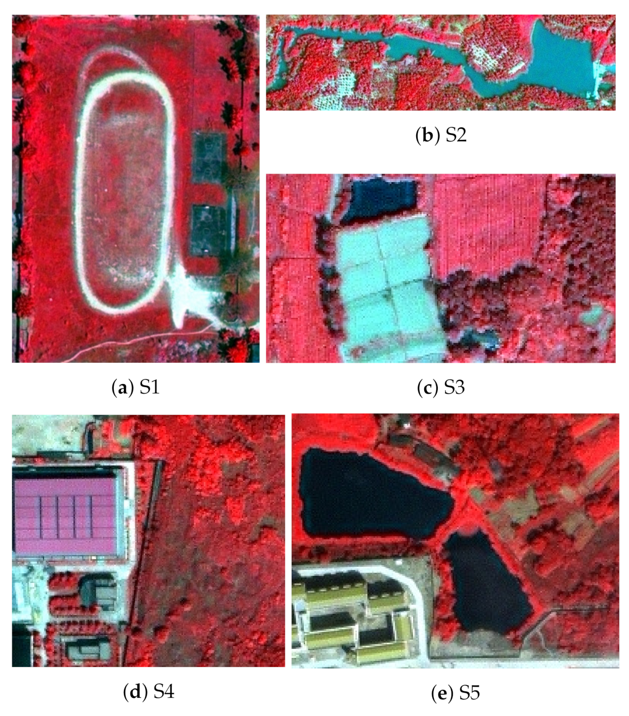
Figure 5.
Five subsets from dataset of D1 and D2.

Figure 6.
Segmentation by setting four different threshold applied for generating spectral-index markers based on NDVI.
Figure 6.
Segmentation by setting four different threshold applied for generating spectral-index markers based on NDVI.

Figure 7.
Segmentation by setting four different threshold applied for generating spectral-index markers based on NDWI.
Figure 7.
Segmentation by setting four different threshold applied for generating spectral-index markers based on NDWI.

Figure 8.
Watershed segmentation by Hill-Marker with the parameter of being 10.

Figure 9.
One-dimension simulated spectral response for thresholding under different values.

Figure 10.
The number of segmentations when the threshold was selected from the range of on subset image.
Figure 10.
The number of segmentations when the threshold was selected from the range of on subset image.

Figure 11.
The optimal image segmentation by automatically selecting the threshold of spectral indices’ KDE.
Figure 11.
The optimal image segmentation by automatically selecting the threshold of spectral indices’ KDE.

Figure 12.
The , , and of segmentation with different scale parameters on subset image of S1 (a), S2 (b), S3 (c), S4 (d), and S5 (e).
Figure 12.
The , , and of segmentation with different scale parameters on subset image of S1 (a), S2 (b), S3 (c), S4 (d), and S5 (e).

Figure 13.
The relationship between the scale and corresponding local variance of regions marked by NDVI for subset images of S1, S2, S3, S4, and S5 under different weighted neighborhood sizes from the interval of [3, 19].
Figure 13.
The relationship between the scale and corresponding local variance of regions marked by NDVI for subset images of S1, S2, S3, S4, and S5 under different weighted neighborhood sizes from the interval of [3, 19].

Figure 14.
The curve of , , and with segmentation number under SI-marker and Hill-marker watershed segmentation methods and MSR method on dataset of D1 (a–c) and D2 (d–f), respectively.
Figure 14.
The curve of , , and with segmentation number under SI-marker and Hill-marker watershed segmentation methods and MSR method on dataset of D1 (a–c) and D2 (d–f), respectively.

Figure 15.
The optimal segmentation result of datasets D1 and D2 based on the SI-marker method, the Hill-marker watershed segmentation method, and the MRS method. (a) SI-marker method; scale = 10; (b) SI-marker method; scale = 20; (c) Hill-marker method; scale = 60; (d) Hill-marker method; scale = 300; (e) MRS method; scale = 200; shape = 0.2; (f) MRS method; scale = 400; shape = 0.5.

Figure 16.
The segmentation result of Regions A, B, C, D, and E of dataset D1 based on the SI-marker method, the Hill-marker watershed segmentation method, and the MRS method.
Figure 16.
The segmentation result of Regions A, B, C, D, and E of dataset D1 based on the SI-marker method, the Hill-marker watershed segmentation method, and the MRS method.

Figure 17.
The segmentation result of Regions F, G, H, and I of dataset D2 based on the SI-marker method, the Hill-marker watershed segmentation method, and the MRS method.
Figure 17.
The segmentation result of Regions F, G, H, and I of dataset D2 based on the SI-marker method, the Hill-marker watershed segmentation method, and the MRS method.


Table 1.
The range of spectral indice, including NDVI and NDWI, on five subset images.
| NDVI | NDWI | |
|---|---|---|
| SI-1 | [161, 189] | [162, 209] |
| SI-2 | [94, 183] | − |
| SI-3 | [122, 178] | [195, 216] |
| SI-4 | [128, 177] | − |
| SI-5 | [149, 194] | [150, 154] |
Publisher’s Note: MDPI stays neutral with regard to jurisdictional claims in published maps and institutional affiliations. |
© 2022 by the authors. Licensee MDPI, Basel, Switzerland. This article is an open access article distributed under the terms and conditions of the Creative Commons Attribution (CC BY) license (https://creativecommons.org/licenses/by/4.0/).
Share and Cite
MDPI and ACS Style
Wang, K.; Chen, H.; Cheng, L.; Xiao, J. Variational-Scale Segmentation for Multispectral Remote-Sensing Images Using Spectral Indices. Remote Sens. 2022, 14, 326. https://doi.org/10.3390/rs14020326
AMA Style
Wang K, Chen H, Cheng L, Xiao J. Variational-Scale Segmentation for Multispectral Remote-Sensing Images Using Spectral Indices. Remote Sensing. 2022; 14(2):326. https://doi.org/10.3390/rs14020326
Chicago/Turabian StyleWang, Ke, Hainan Chen, Ligang Cheng, and Jian Xiao. 2022. "Variational-Scale Segmentation for Multispectral Remote-Sensing Images Using Spectral Indices" Remote Sensing 14, no. 2: 326. https://doi.org/10.3390/rs14020326
Note that from the first issue of 2016, this journal uses article numbers instead of page numbers. See further details here.