
Change Target Extraction Based on Scale-Adaptive Difference Image and Morphology Filter for KOMPSAT-5


Korea Aerospace Research Institute, 169-84, Gwahak-ro, Yuseong-Gu, Daejeon 34133, Korea
*
Author to whom correspondence should be addressed.
Remote Sens. 2022, 14(2), 245; https://doi.org/10.3390/rs14020245
Submission received: 28 November 2021
/
Revised: 21 December 2021
/
Accepted: 29 December 2021
/
Published: 6 January 2022
(This article belongs to the Special Issue Object-Based Classification Using Multi-Source Satellite Image Time Series)
Abstract
:Multitemporal synthetic aperture radar (SAR) images have been widely used for change detection and monitoring of the environment owing to their competency under all weather conditions. However, owing to speckle backgrounds and strong reflections, change detection in urban areas is challenging. In this study, to automatically extract changed objects, we developed a model that integrated change detection and object extraction in multiple Korean Multi-Purpose Satellite-5 (KOMPSAT-5) images. Initially, two arbitrary L1A-level SAR images were input into the proposed model, and after pre-processing, such as radio calibration and coordinate system processing, change detection was performed. Subsequently, the desired targets were automatically extracted from the change detection results. Finally, the model obtained images of the extraction targets and metadata, such as date and location. Noise was removed by applying scale-adaptive modification to the generated difference image during the change detection process, and the detection accuracy was improved by emphasizing the occurrence of the change. After polygonizing the pixel groups of the change detection map in the target extraction process, the morphology-based object filtering technique was applied to minimize the false detection rate. As a result of the proposed approach, the changed objects in the KOMPSAT-5 images were automatically extracted with 90% accuracy.
1. Introduction
Synthetic aperture radar (SAR) employs active electromagnetic waves in the microband that have high transmittance in the atmosphere and are less affected by weather conditions than optical images [1,2]. Owing to these advantages, SAR data are becoming increasingly significant and have been widely used in military and monitoring applications.
By definition, change detection is a technique that identifies changes in status by performing quantitative analysis from the same geographical area [3], which allows for the monitoring of natural disasters, such as earthquakes [4] and flooding [5], as well as the observation of the flow of changes in the urban area. Change detection based on multitemporal, multispectral, and multisensory imagery has been developed over several decades, and has aided in timely and comprehensive planning and decision making. In addition, owing to its high ability to penetrate cloud cover, SAR is widely used for change detection [6] in remote sensing. The general SAR change detection proceeds through the following stages: (1) preprocessing, (2) difference image (DI) generation, and (3) change detection [7,8].
The primary purpose of preprocessing is to reduce noise, make radiometric and geometric corrections, and coregister multiple images [9]. Speckle noise reduction is a critical step because it may yield unreliable change detection results if performed inaccurately [10,11]. Frost filtering [12] and nonlocal, deep learning methods have been developed to reduce speckle noise in SAR images [13].
In the DI generation step, two registered and corrected images were compared pixel-by-pixel. The most straightforward method for generating a DI is to apply a subtraction operation to the two images. However, this method leads to numerous false changed pixels owing to speckle noise and increases the false alarm rate in the subsequent detection procedure. As described in Li et al. [14], the log-ratio operation is a better DI generating approach than the subtraction operation because it can transform multiplicative noise into additive noise and is less sensitive to radiometric inaccuracies. However, log-ratio operations compress modified pixels at high intensities [15], which is particularly problematic for structural objects, such as buildings and vehicles. To improve analysis performance and the noise robustness of DI, numerous combination methods have been proposed [10]. The most commonly acquired improved DI values are mean-ratio DI [16], neighbor-based ratio (NR) DI [17] and Gauss ratio operator [18]. These methods increase the change detection accuracy by combining local spatial information with a mean operation. However, because there are no reference maps or prior knowledge of the image in these methods, it is difficult to determine the optimal window size for the area of interest. In addition, because these methods do not fully utilize spatial information, the final results can be noisy in some cases. Bovolo and Bruzzone [19] used wavelet decomposition on log-ratio images to aggregate multiscale image information and preserve the change details, and Wang et al. [20] introduced a random field based method. Zhuang et al. [21] used heterogeneity to adaptively select the geographical homogeneity neighborhood and a temporal adaptive technique to determine multitemporal neighborhood windows. The new DI reduced the negative effects of noise while preserving the edge details. From the discussion of the aforementioned improved approaches, it can be inferred that combining different DIs or employing neighborhood information may aid in improving change detection performance. Colin et al. [22] proposed a coefficient of variation method and criteria for detecting changes in different data types, such as satellite and unmanned aerial vehicle SAR data.
Recently, deep-learning-based methods have achieved significant success in fields where remote sensing has been applied. In general, machine-learning-based change detection can be divided into supervised and unsupervised approaches [23]. The lack of ground reference data and labor intensive manual labeling processes are major difficulties in the supervised approach [24]. Shu et al. [25] suggested an unsupervised patch based method to iteratively learn the features of changes and reduce the noise effect on the change detection result.
As high resolution SAR images have been acquired with the development of SAR technology, accurate and quick target detection has become a popular topic [26,27]. A target is the object of interest in target detection, such as a vehicle or a ship. In contrast, clutter is the environment, such as land, sea, or trees; targets can be differentiated from clutter provided that imperfections in the images such as noise can be appropriately eliminated or mitigated.
The constant false alarm rate (CFAR) approach, which reorganizes the pixel-level intensity differences between the targets and clutter based on a statistical model, has been the most widely utilized method for target detection owing to its advantages of low-cost computation and adaptive threshold determination [28]. Based on the strategy used to implement the CFAR technique, there are various strategies, such as the cell averaging CFAR (CA-CFAR) [29], the smallest of CFAR (SO-CFAR) detector [30], and adaptive and fast CFAR(AAF-CFAR) [31]. These methods recognize targets based on the difference between the target and the background clutter using statistical models. However, because the observation situation differs, statistical models of clutter, such as the Gaussian and gamma log-normal, are not well suited to some cases, and the accuracy of CFAR is low. In addition, unpredictable factors can cause a phenomenon that exceeds the threshold, and when the model and clutter do not match well, the detection accuracy of the CFAR may also decrease. Therefore, in a complex scenario, the detector performance may degrade, which implies that a different CFAR should be applied to each image or characteristic of the SAR [32]. Xie and Wei [33] explored the region of interest of a mask, which was obtained from the geographical information system, and used image data for detection. Liao et al. [34] divided SAR images into N subimages, and the pixels of the desired target were extracted by the thresholds of the different parts.
To the best of our knowledge, this is the first study to propose an integrated model that can automatically extract changed objects from multiple Korean Multi Purpose Satellite (KOMPSAT-5) images. The main contributions of this study are summarized as follows:
- To improve the change detection performance, a scale-adaptive DI modification method was proposed. This method can be applied regardless of the image complexity or resolution because it performs a scalable transformation of the overall DI. Unlike existing techniques, the proposed algorithm does not require a sliding window or region of interest selection. Hence, it can be processed at a high speed, regardless of the size of the input image.
- The candidate pixel groups were individualized to extract the object of interest from the area where the change occurred, and a morphology-based filtering method was applied. The proposed model can extract a target with high performance and exhibits robust characteristics regardless of noise.
- Change detection and object extraction algorithms were integrated to automatically extract change objects for an arbitrary pair of KOMPSAT-5 images; the model provided the resulting image along with the metadata of the extracted objects, such as location, date, and morphology information.
The remainder of this paper is organized as follows. Section 2 describes the experimental setup and dataset. Section 3 presents the proposed change detection method and experimental results. Section 4 introduces the proposed target extraction method and performance. The integrated model performance and contribution are presented in Section 5 and the conclusions are drawn in Section 6.
2. Experimental Setup
In this study, we developed an automatic changed target extraction model for KOMPSAT-5 images. The model comprises the proposed change detection and object extraction algorithms; preprocessing of the KOMPSAT-5 images was also performed.
2.1. Dataset
The KOMPSAT-5 was first launched in 2013 to provide SAR images for geographic information applications and disaster monitoring systems in Korea. The payload of KOMPSAT-5 includes an X-band (9.66 GHz) SAR system for multimodal observations. The orbit repeat cycle of KOMPSAT-5 is 28 days. Table 1 lists the specifications of the [35] dataset. The satellite provides 1 m-resolution in spotlight mode and 3 m-resolution in strip mode.
In this study, we used enhanced high-resolution (EH) mode imagery with a uniform resolution in the range direction. The chosen dataset pairs comprised images taken with a time difference of approximately a month to half a year.
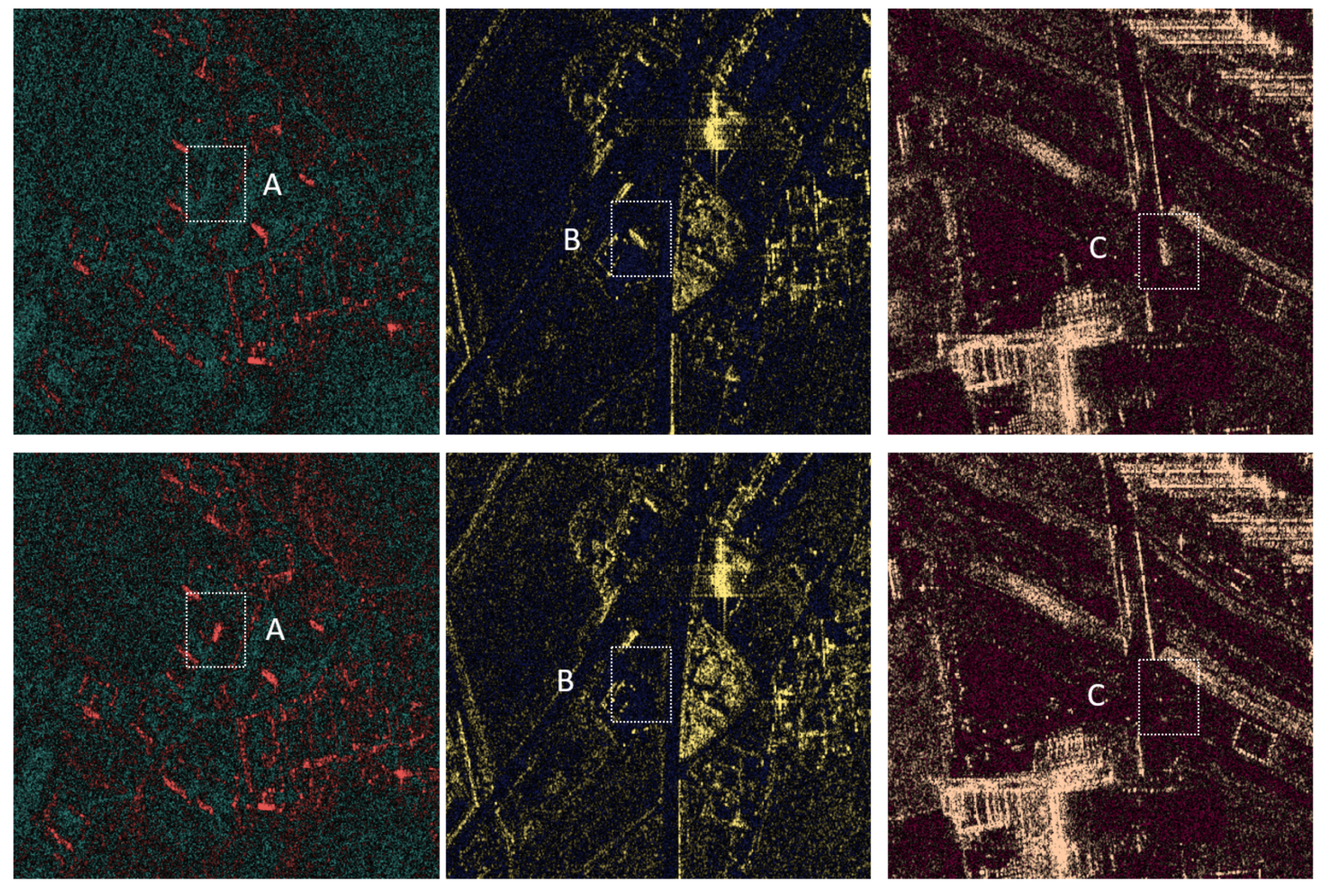
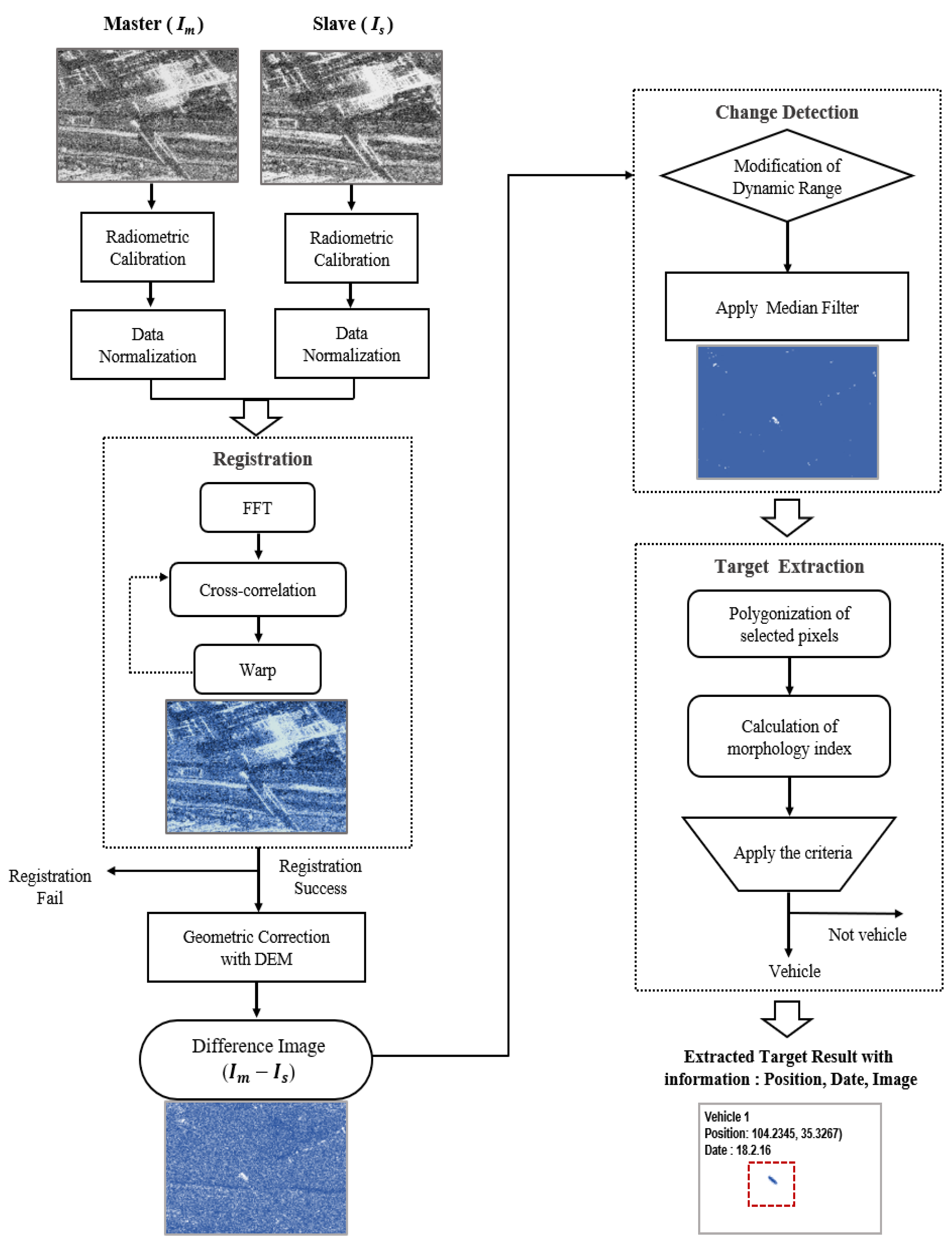
Every dataset had the same conditions (beam mode, polarization, looking mode, and path direction) but with different dates from 2018 to 2019. Each dataset comprised two multitemporal images in the EH mode and level 1A. Level 1A is a process involving spectral correlation similarity, a single-look complex, and slant range. The original KOMSPAT-5 files had a maximum size of 10,000 × 10,000 pixels and approximately occupy 1.5 GB per scene. After data acquisition, if the original image contained a wide range of artifacts due to azimuth ambiguity or excessive layover, it was removed from the analysis list during the data cleaning process. We constructed a ground truth set of SAR images, and optical images were used to confirm the model performance. Figure 1 shows an example of ground truth sets. All metadata were processed in each step with images, such as calibration coefficients and resolution, which were used in the radio calibration and feature extraction steps, respectively. Finally, auxiliary information, such as the date and coordinates of the extracted target location, were provided in the extraction target result. The entire process of extracting changed targets from a pair of KOMPSAT-5 images is shown in Figure 2.
2.2. Preprocessing
In the preprocessing step, we first performed radiometric calibration, which is the process of objectively quantifying each image by calculating the net reflection value for the topography and ground features. Equation (1) derived from the final updated KOMPSAT-5 SAR processor and the absolute radiation correction results described by Yang and Jeong [36] were applied in the radiometric calibration.
Here, is the calibration constant; is the rescaling factor; and and are the real and imaginary pixel values at the ith row and jth column, respectively. N is the number of pixels, and are the column and line pixel spacing, and is the local incidence angle. All variables in Equation (1) are derived from the auxiliary data (.xml).
Meanwhile, even under the assumption that imaging conditions, such as attitude and orbit, are similar, it is impossible to obtain a pair of images with perfectly identical quality owing to the scattering characteristics of the terrain. Here, the ’primary’ image indicates an earlier date among the input pairs, and the ’secondary’ image indicates a later date. This inevitable difference affects the final performance of the change detection. Therefore, for accurate change detection, it is necessary to normalize the dynamic range in pairs of images [37]; the intensity distribution of each radiometrically calibrated image is normalized to have a distribution of [0, 1].
3. Proposed Change Detection Method and Performance
3.1. Difference Image Generation
After preprocessing, as described in Section 2.2, the data of the primary and secondary images were distributed within the same dynamic range; however, the two images still had geometrical position errors. For precise image coregistration and correction of geometrical errors, we implemented a two-step registration method; the registration involved fast Fourier transform (FFT) and cross-correlation. FFT-based registration was based on the Fourier shift theorem [38], and the amount of translation required for the secondary image to precisely fit the primary image was converted into a phase difference in the frequency domain. Subsequently, by using the inverse FFT, the phase correlation can be computed using Equation (2),
where ; and are the corresponding FT of and , respectively; and denotes the inverse FT; * denotes the complex conjugate. In this step, the position mismatch error of the order of 103 pixels was reduced to subpixels.
Once the secondary image was approximately aligned using FFT translation, additional fine registration was required to increase the detection accuracy. First, the primary and shifted secondary images were stacked based on the geometry of the primary image. As a result of the stack operation, the two images obtained similar dimensions and shared geometrical information, such as the orbit. When the two images were aligned, the band data of the shifted secondary image were resampled into the primary image using the nearest interpolation.
Furthermore, the fine registration and cross-correlation method were executed by maximizing the coherence. One thousand ground control points (GCPs) were randomly selected to calculate the correlation. Beginning with the coarse registered secondary GCPs, the optimal subpixel shift was computed such that the new secondary image at the new GCP position provided maximum coherence with the primary image within the defined sliding window. Once the valid GCPs were selected using the least squares method that maps the new pairs of GCPs, we computed the polynomial in the order of 1 in an iterative manner. During the processing, the root mean square (RMS) and standard deviations of the residuals were computed. Only GCPs smaller than the mean RMS were used. Finally, the GCP pairs were filtered at a threshold of 0.05, and the final warp function was computed using the remaining GCP pairs.
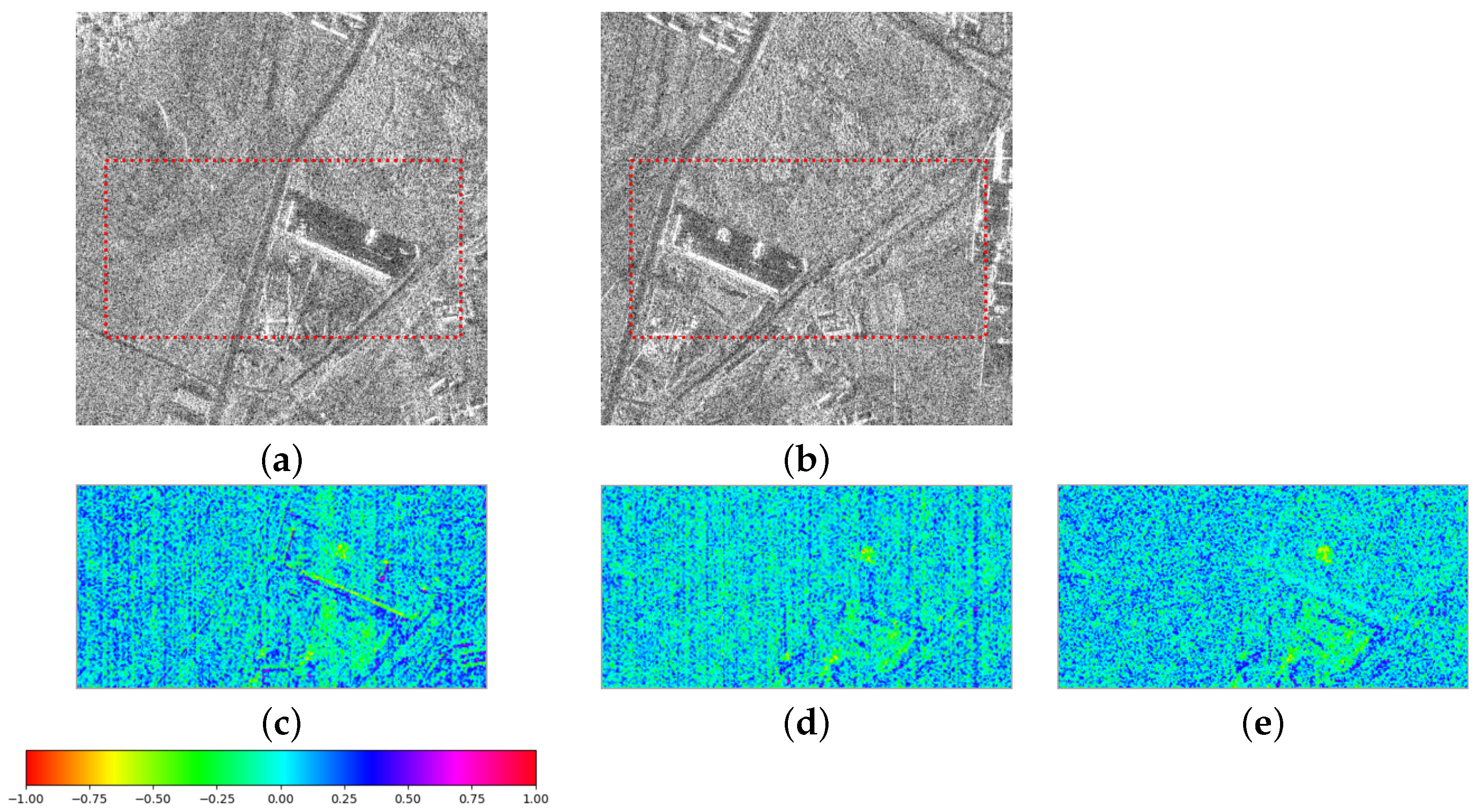
The primary image () in Figure 3a and secondary image () in Figure 3b were obtained from June 2018 and September 2018. The DI is the result of linear subtraction of the secondary from the primary image. The structure shown in Figure 3a,b (i.e., the red-dotted box), appears in a different position; it denotes the value of the positional error between the two images. To verify the performance of our proposed registration method, we compared the results with those of two other methods. The first method suggested matching the two images using the orbit and precise external digital elevation model (DEM) data. Each primary and secondary image was required to be resampled in a bilinear method to be matched based on the DEM. We used the external Shuttle Radar Topography Mission (SRTM) 1 arc sec DEM [39] file in the Geotiff format. As the previously used image of the KOMPSAT-5 was taken with precise orbit processing at the level product step, the additional orbit matching process was not required. As a result of the DEM based registration, as depicted in Figure 3c, we observed an inconsistency as the roads or structures appeared as two lines. The DI by the second method in Figure 3d was generated by the cross-correlation method; in this method, FFT was not applied, unlike our proposed two-step registration. This method is widely used, and unlike the DEM method, the matching performance is satisfactory, as shown in Figure 3d. However, a peculiar pattern may occur during the resampling or warp process. In addition, when the initial position error between the pair of images is large, registration fails. The results of our two-step coregistration are shown in Figure 3e. Unlike the other two methods, the overlapping phenomenon completely disappeared, and a clear DI could be obtained, as depicted in Figure 3e.
Subsequently, the geometric range can be distorted in SAR images because of the tilt angle of the sensor and topographical variations of the scene. As we used a pair of Level 1A images to create the DI, terrain correction was required to compensate for these distortions such that the geometric representation of the image would be as close as possible to the real world. The same DEM data used for terrain correction were also used.
3.2. Scale-Adaptive DI Modification Method
In change detection, a feature that exists only in the primary or secondary image shows a strong pattern, but the parts that are not removed, such as noise or background, appear in both images with different intensity levels. In addition, the high performance of change detection implies that as much noise as possible is removed, and only the parts with significant differences are extracted from the two images. The log-ratio intensity method is widely used for change detection in SAR. However, instead of log-ratio intensity, we propose a scale-adaptive modification of DI for high-performance change detection. When generating DI, the intensity distribution refers to the linear difference − between the two scaled images that has a value in the range [0, 1], and the DI that has a value in the range [−1, 1].
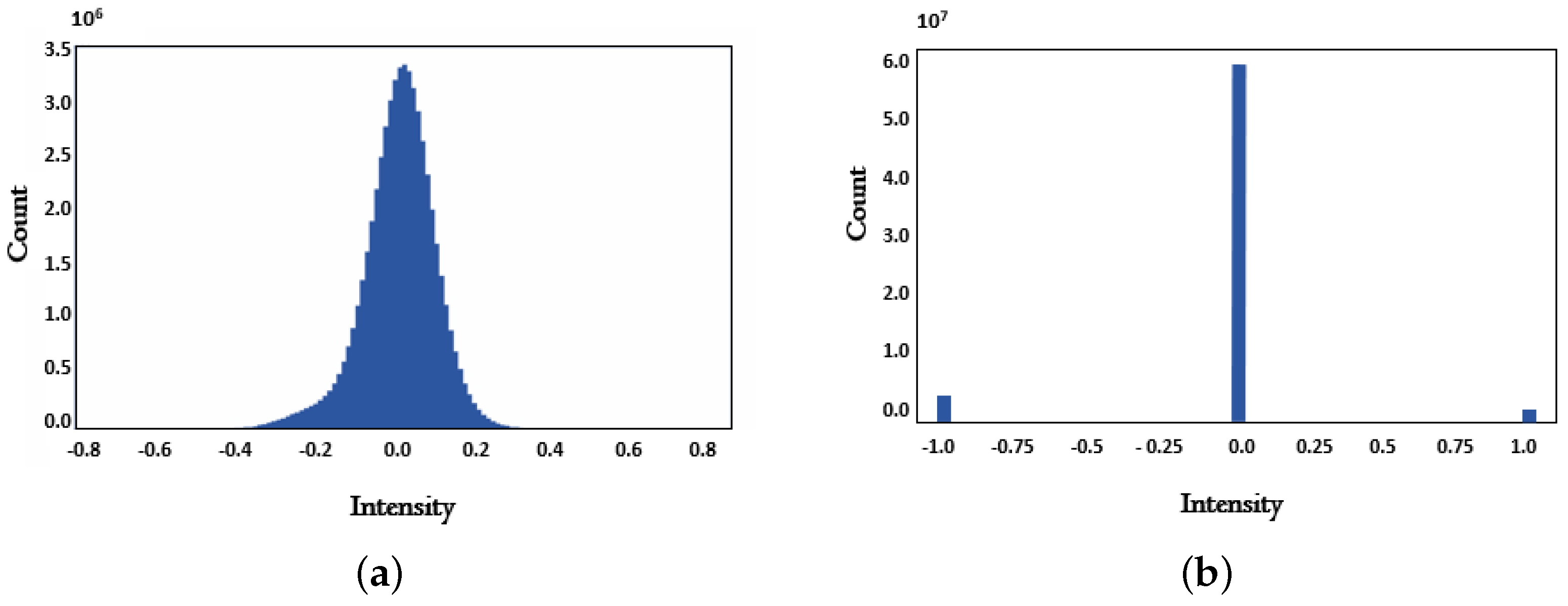
As shown in Figure 4a, in the dynamic range distribution of the DI, the left tail of the graph denotes the part that exists only in the secondary image and the right tail corresponds to the primary image. The middle part in Figure 4a is present in both images; therefore, it can be considered to be noise or an unchanged part similar to the background in both images. As our final goal was to detect the changed objects in the two images, it was necessary to maximize the difference by analyzing the dynamic range and modifying the distribution by applying Equation (3).
where represents the normalized difference map value. According to Equation (3), we set the convert values exceeding 30% of the maximum value in the original DI () to 1, and the values below 0.3 of the minimum value to −1 (refer to Figure 4b). Here, 30% is the optimal value obtained through the experimental results while changing the corresponding parameter by 2%. If the processing criterion is less than 30%, the change in the target feature size is drastically reduced. However, when it is higher than 30%, the background noise increases; the number of extraction candidates sharply increases; and ultimately, the number of false positives increases.
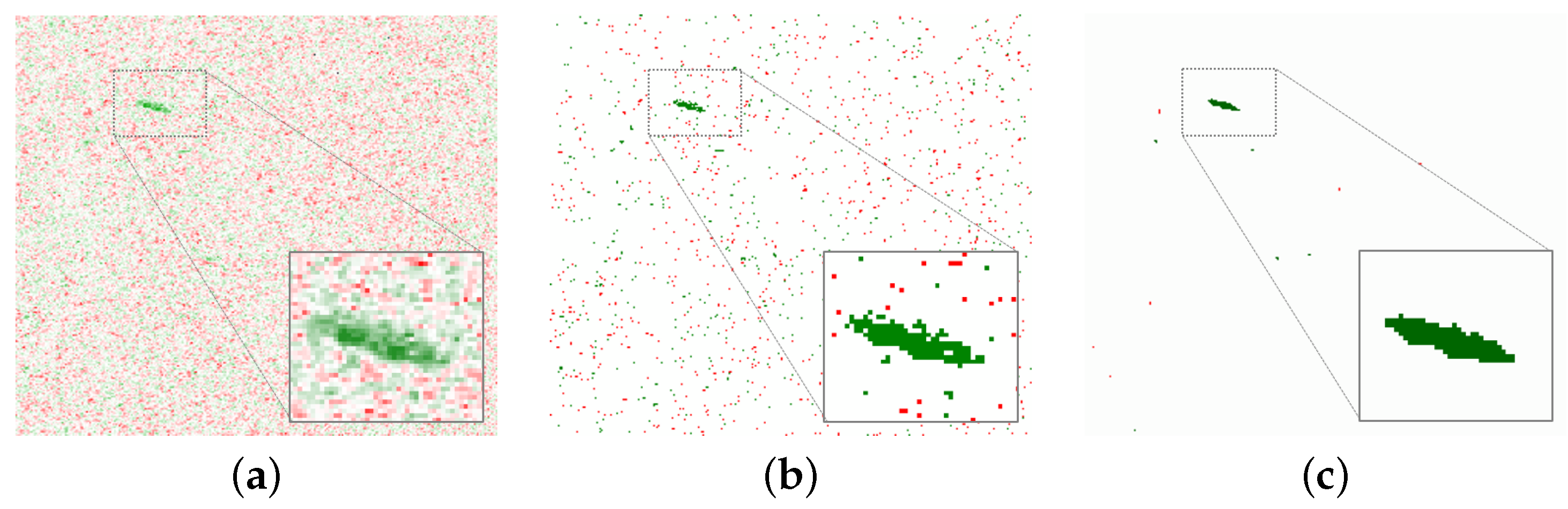
Thus, if the scaling of the entire intensity distribution of DI is adjusted and changed, the overall intensity of the change can be clearly distinguished. In addition, the background or noise present in both images is removed and, in particular, the degree of change is maximized by discretely changing the continuously distributed change scaling. When Equation (3) was applied to the original DI in Figure 5a, more than 99% of high-intensity speckle noise was removed as shown in Figure 5b.
In the next step, the median filter, as described in Equation (4), was adopted to remove the remaining noise and maintain the shape of the object by smoothing.
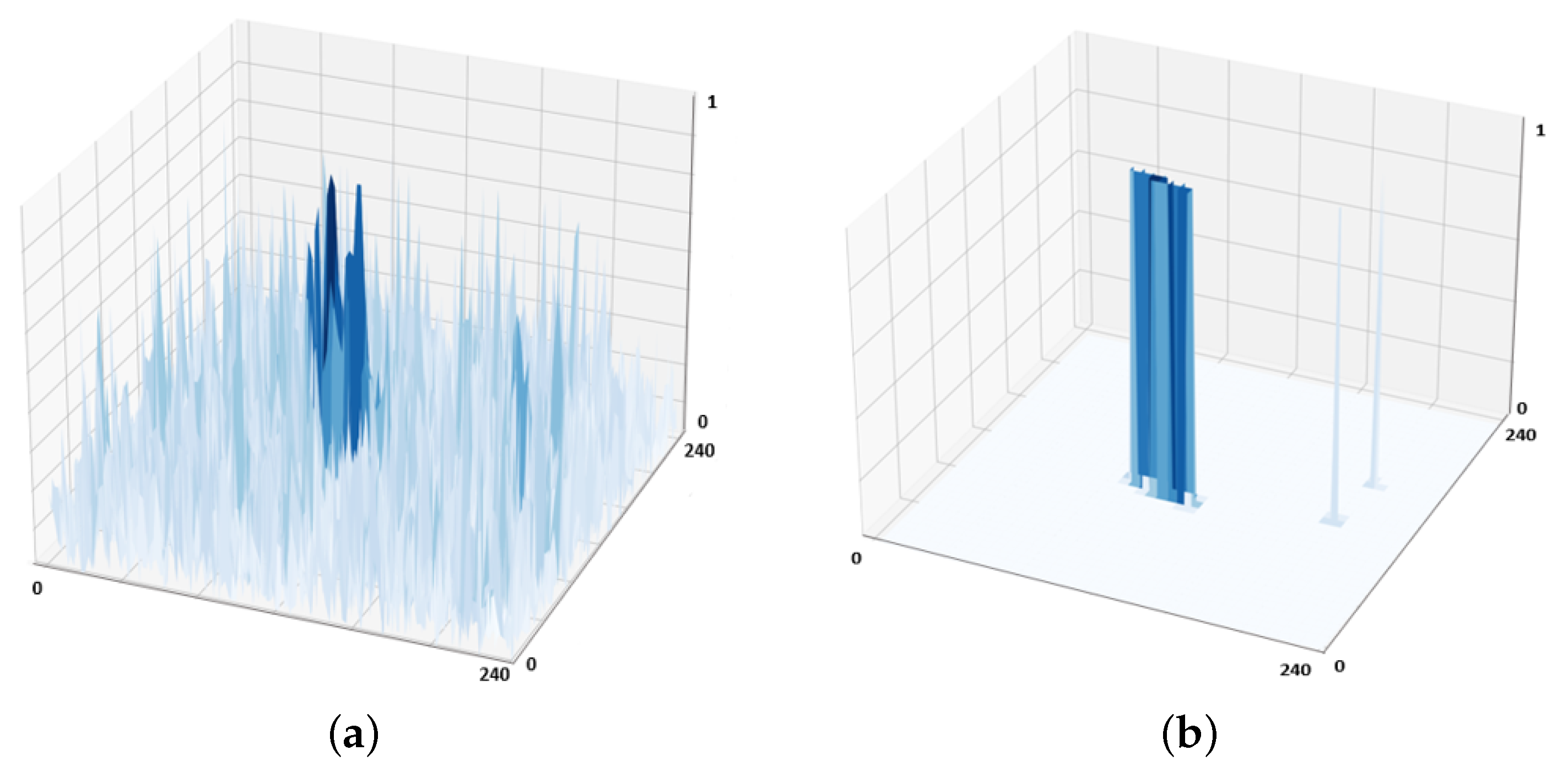
The median filter [40] is a nonlinear method that defines the median value within a set window area and removes outliers that are beyond the sorted values. The bottom right box in Figure 5c shows the effects of the median filter that highlights the shape by filling the pixels of the changed objects displayed in green and removing almost all the background pixels. Through this process, a clear change detection map was obtained. As shown in Figure 6, after applying the scale-adaptive modification and median filter proposed to DI, it can be confirmed that the clutter part of the noise around the target was completely removed, and the features of the targets were obtained.
4. Proposed Desired Target Extraction Method and Performance
This section introduces the process of extracting target candidates from the change detection map.
4.1. Feature-Based Polygonization of Changed Pixels Groups
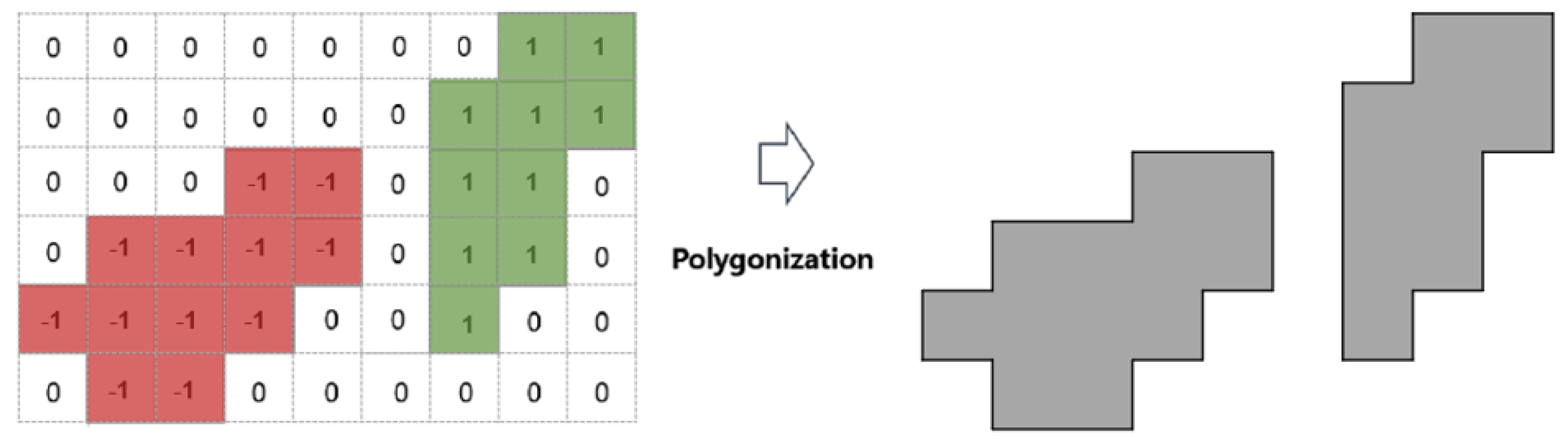
As described in Section 3.2, the pixels in the change detection map had −1, 0, and 1 in the same dimension. The raster image in the change detection was mapped into each valued dimension, −1, 0, and 1; we named this process reclassification. During the reclassification process, the raster image in the change detection map is mapped to each valued dimension.
In this process, neighboring pixels with the same value comprise one polygon. Through polygonization of the pixel groups on the dimension map, each pixel group can be analyzed as an object with its shape. As shown in Figure 7, zero-valued pixels were considered to be noise; therefore, they were not converted into polygons, and all corresponding information was deleted. Only two polygon sets, one composed of −1 valued (red) pixels and the other of 1 valued (green) pixels, were created and considered as candidate groups of objects.
When a change detection map was created using two KOMPSAT-5 images and converted into a polygon set, the number of polygons in each set was approximately –. Therefore, it is necessary to apply an algorithm that focuses solely on meaningful target polygons.
4.2. Morphology-Based Target Extraction Method
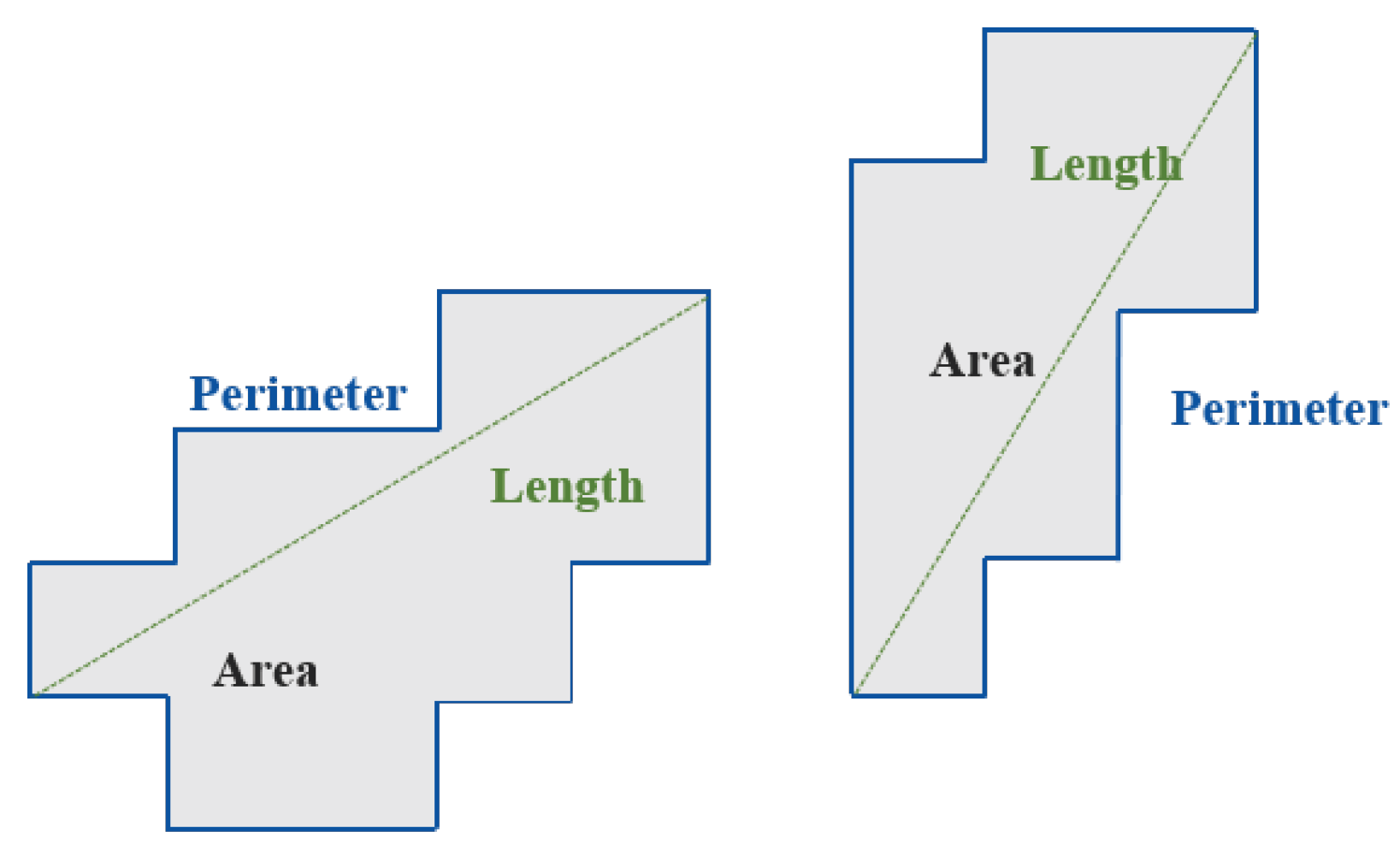
In this study, the target of interest was a vehicle at an urban site. We collected more than 300 cars as the ground truth dataset and analyzed their morphological characteristics, such as area, length, and shape index (SI). The SI was calculated based on the combination of the perimeter and area of each polygon using the following formula [41]:
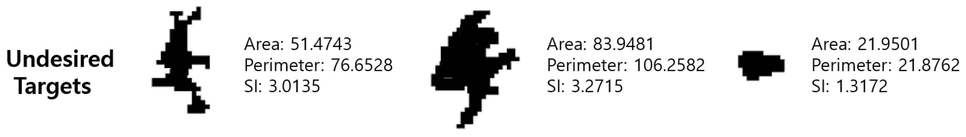
where is the perimeter of the input polygon ith and is the area of the ith input polygon, respectively. When the SI value is close to 1, the polygon has a form close to the regular form, such as a circle or square, whereas the polygon has an elongated atypical form when the SI value is large. The SI is applied for the first time to target extraction in SAR images in this study and is used as a discriminator to differentiate between undesired and target objects. The criteria for each parameter were also set through morphological analysis of the ground truth data. The morphological parameters are shown in Figure 8.
Among the parameter filters, we first applied the ’area’ filter. Only polygons that were larger than the threshold (=18) area were considered as the candidate objects of interest; smaller ones were considered to be errors and were removed.
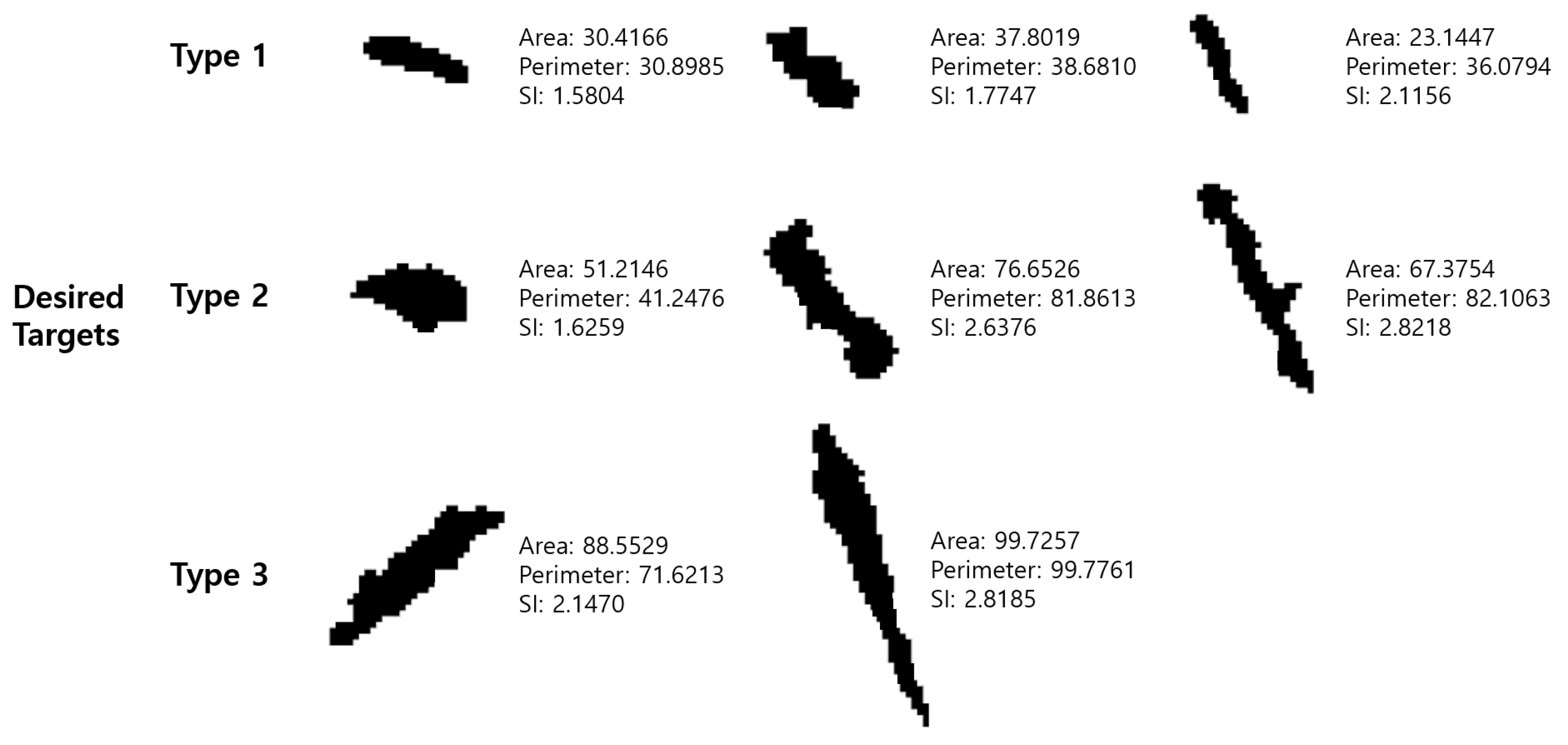
The shape of the desired objects was close to a rectangle, and as the size of the object increased, a more elongated rectangular shape was obtained; the horizontal lengths of the small and large objects were similar, but the vertical length increased. Therefore, a large vehicle has a higher SI value than a small vehicle. The object we intend to extract in this step is not the original shape; thus, there is an inevitable change in the shape of the objects. The second criteria for polygon selection are listed in Table 2. Considering image resolution and dataset uncertainty, we categorized the object types into three categories: type 1 denotes small vehicles; type 2 denotes medium sized vehicles, such as buses and trucks; and type 3 denotes large-sized objects, such as heavy equipment vehicles. Examples of the three types of desired/undesired objects and their morphological information are depicted in Figure 9 and Figure 10.
Finally, to distinguish meaningful targets from incorrect objects, such as artificial structures, the long axis of the polygon was calculated as the length of the target, as depicted in Figure 8. After creating a line connecting all points of the polygon, the maximum length of the polygon was set as the longest line. In this study, only polygons longer than 10 m (10 m-size) were selected as the final target object.
4.3. Target Extraction Performance
Our test sets of KOMPSAT-5 images are in the HDF5 format, and level 1A of size and 10 test pairs of the images acquired between January 2018 and August 2020 were randomly selected. To validate our method, we counted all candidate targets in the results of each filter step. Table 3 describes the overall performance of the target extraction process and the final precision of changed target extraction.
In this test, we evaluated the performance of morphology-based extraction performance. The initial status in Table 3 represents the number of polygons after the completion of the polygonization process, as described in Section 4.1; more than polygons were considered to be initial target candidates, as described in the 2nd column in Table 3. Compared with the 2nd and 3rd columns in Table 3, approximately 99% of the undesired polygons were removed in the area filtering step. In the SI filtering step described in the 4th column, 18–37% of the objects are filtered out. Finally, we applied the length criteria described in the 5th column. After the SI filter step, the extraction accuracy was increased by removing the wrong targets of similar shapes. As a result, we extracted 0.39% of the ratio of the initial status to objects after applying the cutoff, SI, and length criteria. This implies that the proposed filter works effectively at each step.
5. Integrated Performance and Discussion
The implemented method is intended for changed vehicle extraction from a pair of SAR images. The detector was evaluated on randomly selected 10 pairs of the test set, and the final extraction result was compared with the optical image.
The precision of Equation (6), which is an object extraction performance index, was calculated by comparing the extracted changed objects with the ground truth sheet. We denote the set of correctly detected objects as true positives (TPs), the set of falsely detected objects as false positives (FPs), and missed objects as false negatives (FN). As shown in Table 4, from 10 pairs of arbitrary test sets, an average extraction performance precision of 84%, a recall of 91%, and F1 score of 87% were obtained.
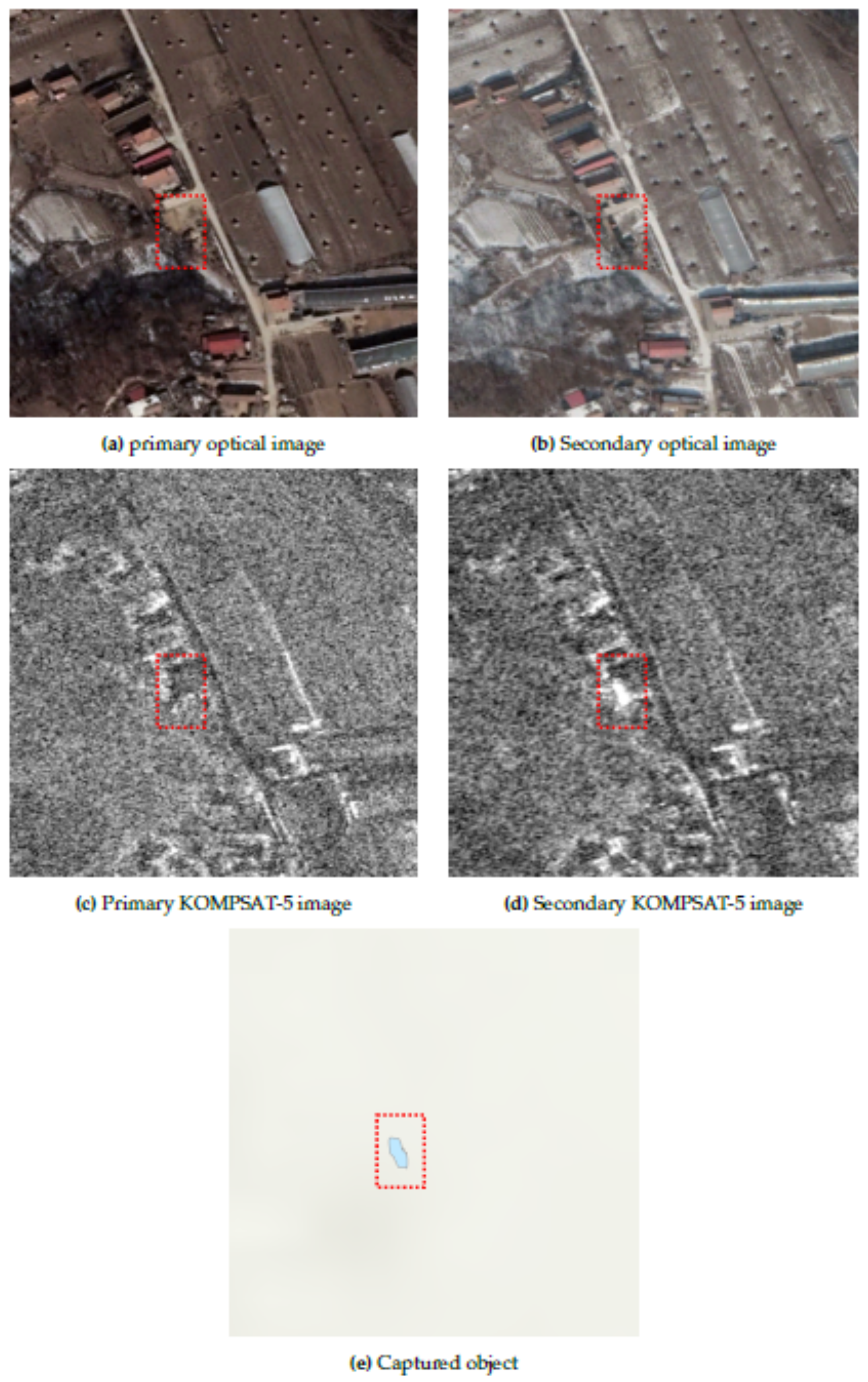
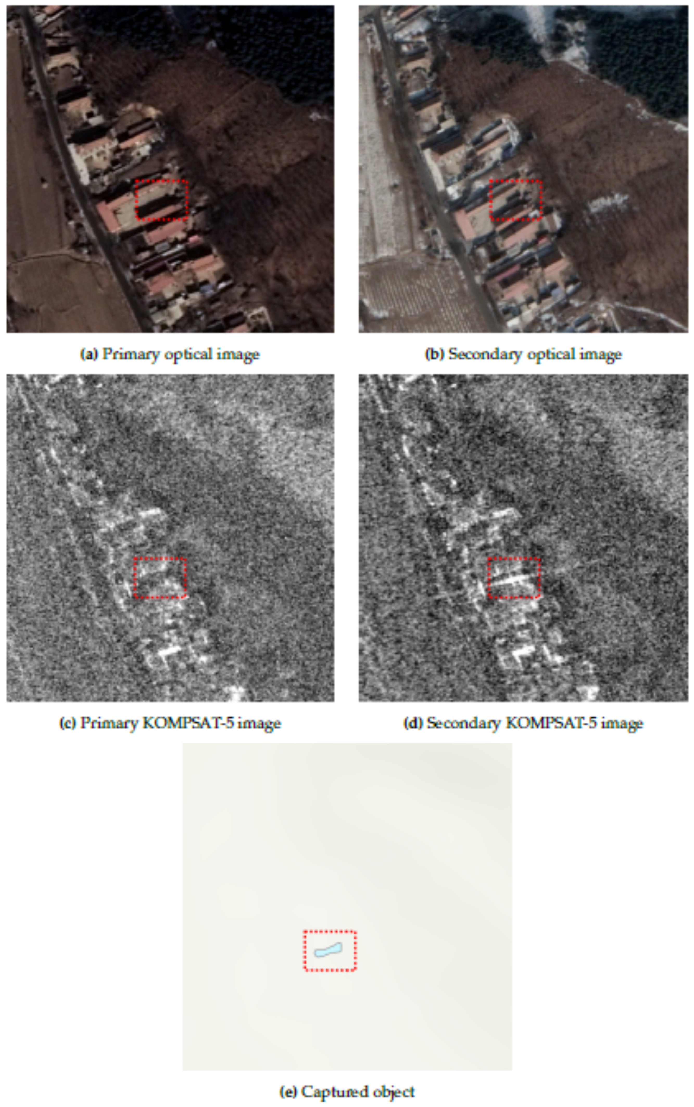
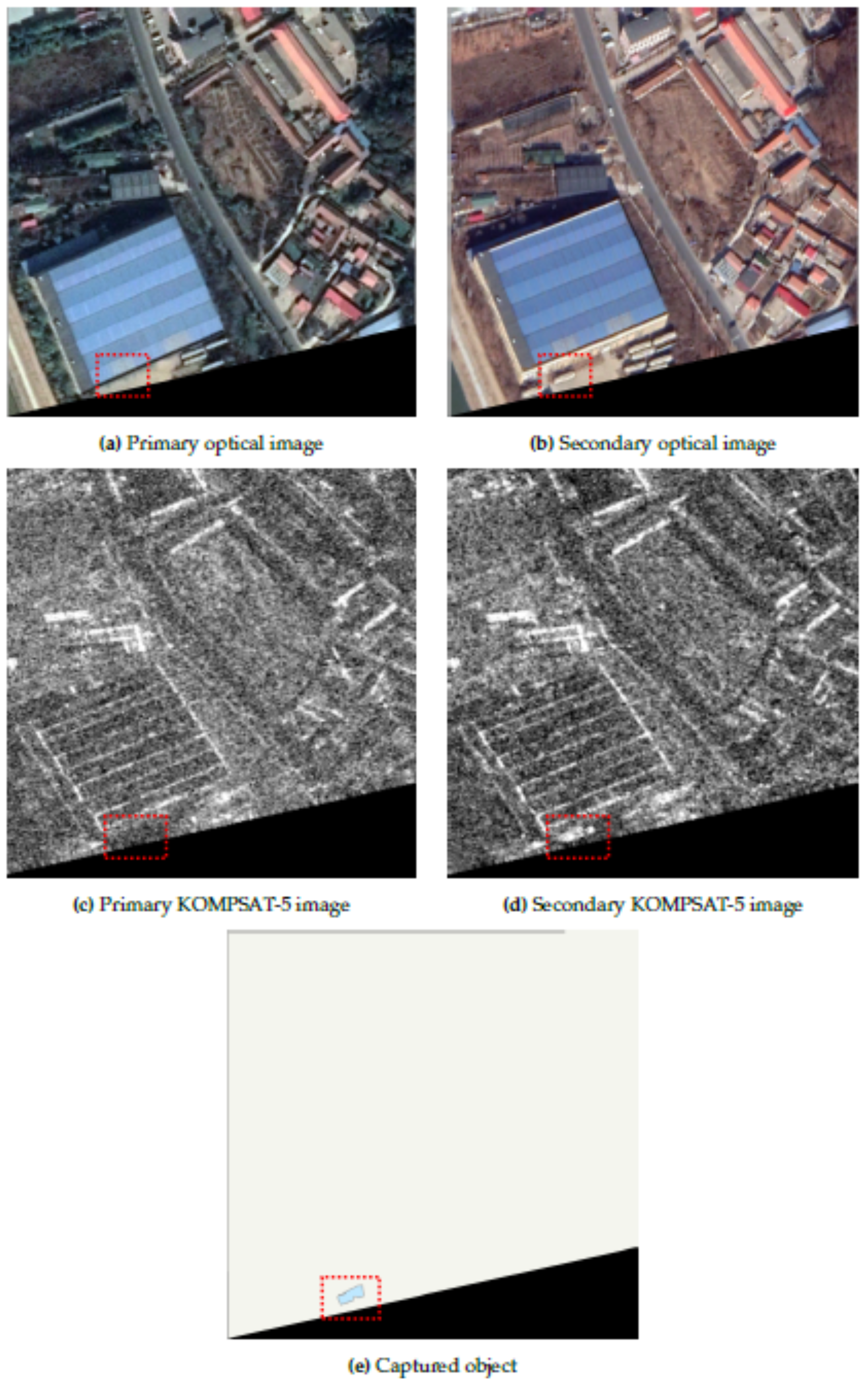
The CNES/Airbus and Maxar [42] optical images were used as auxiliary data to understand the extraction performance. Figure 11, Figure 12 and Figure 13 depict examples of verification of the extraction performance by comparing the developed methodology with optical images. Figure 11a, Figure 12a and Figure 13a are matched optical images with the SAR primary image shown in Figure 11c, Figure 12c and Figure 13c and Figure 11b, Figure 12b and Figure 13b are matched with Figure 11d, Figure 12d and Figure 13d. The red dotted boxes in Figure 11e, Figure 12e and Figure 13e indicate the area from which the change object was extracted.
A large vehicle that was not visible in the red box in Figure 11c appeared in Figure 11d, which is the target we intend to extract. When the proposed model was applied to the primary and secondary images, as shown in Figure 11e, the recently emerged vehicle was extracted, excluding the buildings and roads that existed in both images.
Figure 12e shows the result of extraction from the other set of Figure 12c,d, and the large vehicle found between the complex buildings in the secondary image was accurately extracted. The results showed that the changed vehicle, which appeared in the secondary image, was not detected in the primary. In fact, structures that existed in both the images, such as roads and houses, were not detected. Figure 12 displays the results where only vehicles in the yellow boxes that exist between more complex buildings were detected. In particular, only the target was detected using the proposed method, even though the smearing phenomenon appeared in the secondary image. Similarly, Figure 13 shows that a newly parked vehicle next to the building was accurately detected.
It was confirmed that the automatic detection integrated model (change detection, object extraction) developed in this study effectively extracts the changed target from the two images of KOMPSAT-5 as described above. In the change detection model, a method of applying scale-adaptation correction to the difference image was proposed in order to emphasize the part where the change occurred in two arbitrary images. Scale-adaptation plays a role in highlighting the part where the change occurs in order to differentiate from the speckle noise included in the SAR image and the fixed objects present in both time series data. Through parameter change and multiple tests, the part corresponding to 30% of the maximum/minimum value in the difference image was converted to +/−1, and the other parts were replaced with 0, making it possible to distinguish the change object from the background. The median filter enhances the change detection performance by emphasizing the shape of the change-occurring part and removing the remaining noise. In the object extraction step, by polygonizing the remaining candidate pixel groups in the result of the change detection step, they are transformed into individual objects. As a result, the change detection result was changed to a collection of objects that can analyze individual characteristics. By applying the shape index to the object extraction in the SAR image, we enabled effective extraction based on the morphology feature of the objects of interest. In particular, when objects are extracted from a change detection image (difference image), an object such as a vehicle changes to an irregular shape in the difference step; nevertheless, we were able to extract the desire targets with high performance. We finally integrated the above two change detection/object extraction models including preprocessing into one model, and this model extracts the results within about 5 min for two arbitrary KOMPSAT-5 images. The extraction result image (.img) of the desired targets in which the change has occurred and auxiliary data about the extraction are described as a result. In particular, the model was developed so that auxiliary data of the extracted targets such as date, location, and shape information (length, area, etc.) are described in separate documents (.csv and .shp). It is expected that such an automated extraction model will be helpful in monitoring and calculating statistical data for the region of interest.
In this study, an extraction method was proposed based on a pair of images with the same imaging conditions. However, in the case of SAR, many cases are taken while changing the incidence angle/looking mode. In particular, when the incidence angle is changed, the spacing of pixels for each image changes, making it impossible to analyze with the proposed model. Therefore, to overcome this limitation, we plan to enhance the model in the future, such as by image spacing conversion according to the incidence angle and automatic adjustment of the analysis area that are dependent on the looking mode.
6. Conclusions
In this study, to automatically extract changed objects in multiple KOMPAT-5 datasets, we developed a model that integrated change detection and object extraction for the first time. We adopted scale-adaptive difference image modification to highlight the changed parts. In addition, morphology-based indicators effectively discriminate between desired and undesired objects and improve the final extraction accuracy. The proposed method achieved an accuracy of approximately 90% for changed target extraction from two random SAR images. This integrated model is expected to be effectively utilized for extracting various target-based statistical information from multiple KOMPSAT-5 datasets. However, it remains challenging to reduce the false detection rate when the incidence angles are distinctly different for each image. This yields a difference in pixel spacing between the images, resulting in large positional errors or distortions. Furthermore, owing to the limitation of the image resolution, when the type of vehicle or parking direction is slightly changed, detection poses a difficulty. Therefore, in the future, we will improve the proposed method through the adaptive conversion of pixel spacing or by using a deep-learning technique.
Author Contributions
Conceptualization, Y.C. and J.H.; methodology, Y.C. and J.H.; software, J.H.; validation, D.Y.; formal analysis, Y.C.; investigation, Y.C. and J.H.; resources, Y.C. and J.H.; data curation, D.Y.; writing—original draft preparation, Y.C. and J.H.; writing—review and editing, D.Y.; visualization, Y.C. and J.H.; supervision, S.H.; project administration, Y.C.; funding acquisition, S.H. All authors have read and agreed to the published version of the manuscript.
Funding
This research was funded by the Korea goverment (MSIT).
Conflicts of Interest
The authors declare no conflict of interest.
References
- Curlander, J.C.; McDonough, R.N. Synthetic Aperture Radar; Wiley: New York, NY, USA, 1991; Volume 11. [Google Scholar]
- Brown, W.M. Synthetic aperture radar. IEEE Trans. Aerospace Electron. Syst. 1967, AES-3, 217–229. [Google Scholar] [CrossRef]
- Rignot, E.J.; Van Zyl, J.J. Change detection techniques for ERS-1 SAR data. IEEE Trans. Geosci. Remote Sens. 1993, 31, 896–906. [Google Scholar] [CrossRef] [Green Version]
- Brunner, D.; Lemoine, G.; Bruzzone, L. Earthquake damage assessment of buildings using VHR optical and SAR imagery. IEEE Tran. Geosci. Remote Sens. 2010, 48, 2403–2420. [Google Scholar] [CrossRef] [Green Version]
- Kim, Y.; Lee, M.J. Rapid Change Detection of Flood Affected Area after Collapse of the Laos Xe-Pian Xe-Namnoy Dam Using Sentinel-1 GRD Data. Remote Sens. 2020, 12, 1978. [Google Scholar] [CrossRef]
- Li, L.; Wang, C.; Zhang, H.; Zhang, B.; Wu, F. Urban building change detection in SAR images using combined differential image and residual U-Net network. Remote Sens. 2019, 11, 1091. [Google Scholar] [CrossRef] [Green Version]
- Cui, B.; Zhang, Y.; Yan, L.; Cai, X. A SAR intensity images change detection method based on fusion difference detector and statistical properties. ISPRS Annal. Photogram. Remote Sens. Spat. Inform. Sci. 2017, 4, 439. [Google Scholar] [CrossRef] [Green Version]
- Gao, F.; Liu, X.; Dong, J.; Zhong, G.; Jian, M. Change detection in SAR images based on deep semi-NMF and SVD networks. Remote Sens. 2017, 9, 435. [Google Scholar] [CrossRef] [Green Version]
- Lei, Y.; Liu, X.; Shi, J.; Lei, C.; Wang, J. Multiscale superpixel segmentation with deep features for change detection. IEEE Acc. 2019, 7, 36600–36616. [Google Scholar] [CrossRef]
- Gong, M.; Zhou, Z.; Ma, J. Change Detection in Synthetic Aperture Radar Images based on Image Fusion and Fuzzy Clustering. IEEE Trans. Image Proces. 2012, 21, 2141–2151. [Google Scholar] [CrossRef]
- Li, H.; Gong, M.; Wang, C.; Miao, Q. Self-paced stacked denoising autoencoders based on differential evolution for change detection. Appl. Soft Comput. 2018, 71, 698–714. [Google Scholar] [CrossRef]
- Sun, Z.; Zhang, Z.; Chen, Y.; Liu, S.; Song, Y. Frost filtering algorithm of SAR images with adaptive windowing and adaptive tuning factor. IEEE Geosci. Remote Sens. Lett. 2019, 17, 1097–1101. [Google Scholar] [CrossRef]
- Cozzolino, D.; Verdoliva, L.; Scarpa, G.; Poggi, G. Nonlocal CNN SAR image despeckling. Remote Sens. 2020, 12, 1006. [Google Scholar] [CrossRef] [Green Version]
- Li, Y.; Martinis, S.; Plank, S.; Ludwig, R. An automatic change detection approach for rapid flood mapping in Sentinel-1 SAR data. Int. J. Appl. Earth Observat. Geoinform. 2018, 73, 123–135. [Google Scholar] [CrossRef]
- Zhang, Y.; Wang, C.; Wang, S.; Zhang, H.; Liu, M. SAR image change detection method based on visual attention. In Proceedings of the 2017 IEEE International Geoscience and Remote Sensing Symposium (IGARSS), Fort Worth, TX, USA, 23–28 July 2017; pp. 3078–3081. [Google Scholar]
- Inglada, J.; Mercier, G. A new statistical similarity measure for change detection in multitemporal SAR images and its extension to multiscale change analysis. IEEE Trans. Geosci. Remote Sens. 2007, 45, 1432–1445. [Google Scholar] [CrossRef] [Green Version]
- Argenti, F.; Alparone, L. Speckle removal from SAR images in the undecimated wavelet domain. IEEE Trans. Geosci. Remote Sens. 2002, 40, 2363–2374. [Google Scholar] [CrossRef]
- Hou, B.; Wei, Q.; Zheng, Y.; Wang, S. Unsupervised change detection in SAR image based on Gauss-log ratio image fusion and compressed projection. IEEE J. Select. Top. Appl. Earth Observat. Remote Sens. 2014, 7, 3297–3317. [Google Scholar] [CrossRef]
- Bovolo, F.; Bruzzone, L. A detail-preserving scale-driven approach to change detection in multitemporal SAR images. IEEE Trans. Geosci. Remote Sens. 2005, 43, 2963–2972. [Google Scholar] [CrossRef]
- Wang, F.; Wu, Y.; Zhang, Q.; Zhang, P.; Li, M.; Lu, Y. Unsupervised change detection on SAR images using triplet Markov field model. IEEE Geosci. Remote Sens. Lett. 2012, 10, 697–701. [Google Scholar] [CrossRef]
- Zhuang, H.; Fan, H.; Deng, K.; Yu, Y. An improved neighborhood-based ratio approach for change detection in SAR images. Eur. J. Remote Sens. 2018, 51, 723–738. [Google Scholar] [CrossRef] [Green Version]
- Colin Koeniguer, E.; Nicolas, J.M. Change Detection Based on the Coefficient of Variation in SAR Time-Series of Urban Areas. Remote Sens. 2020, 12, 2089. [Google Scholar] [CrossRef]
- Geng, J.; Ma, X.; Zhou, X.; Wang, H. Saliency-guided deep neural networks for SAR image change detection. IEEE Trans. Geosci. Remote Sens. 2019, 57, 7365–7377. [Google Scholar] [CrossRef]
- Saha, S.; Bovolo, F.; Bruzzone, L. Building change detection in VHR SAR images via unsupervised deep transcoding. IEEE Trans. Geosci. Remote Sens. 2020, 59, 1917–1929. [Google Scholar] [CrossRef]
- Shu, Y.; Li, W.; Yang, M.; Cheng, P.; Han, S. Patch-Based Change Detection Method for SAR Images with Label Updating Strategy. Remote Sens. 2021, 13, 1236. [Google Scholar] [CrossRef]
- Dudgeon, D.E.; Lacoss, R.T. An overview of automatic target recognition. Linc. Lab. J. 1993, 6, 3–10. [Google Scholar]
- Bhanu, B.; Dudgeon, D.E.; Zelnio, E.G.; Rosenfeld, A.; Casasent, D.; Reed, I.S. Guest editorial introduction to the special issue on automatic target detection and recognition. IEEE Trans. Image Proces. 1997, 6, 1–6. [Google Scholar] [CrossRef]
- El-Darymli, K.; McGuire, P.; Power, D.; Moloney, C.R. Target detection in synthetic aperture radar imagery: A state-of-the-art survey. J. Appl. Remote Sens. 2013, 7, 071598. [Google Scholar] [CrossRef] [Green Version]
- Schwegmann, C.P.; Kleynhans, W.; Salmon, B.P.; Mdakane, L. A CA-CFAR and localized wavelet ship detector for sentinel-1 imagery. In Proceedings of the 2015 IEEE International Geoscience and Remote Sensing Symposium (IGARSS), Milan, Italy, 26–31 July 2015; pp. 3707–3710. [Google Scholar]
- Trunk, G.V. Range resolution of targets using automatic detectors. IEEE Trans. Aerosp. Electron. Syst. 1978, 5, 750–755. [Google Scholar] [CrossRef]
- Gao, G.; Liu, L.; Zhao, L.; Shi, G.; Kuang, G. An adaptive and fast CFAR algorithm based on automatic censoring for target detection in high-resolution SAR images. IEEE Trans. Geosci. Remote Sens. 2008, 47, 1685–1697. [Google Scholar] [CrossRef]
- Fei, G.; Aidong, L.; Kai, L.; Erfu, Y.; Hussain, A. A novel visual attention method for target detection from SAR images. Chin. J. Aeronaut. 2019, 32, 1946–1958. [Google Scholar]
- Xie, L.; Wei, L. Research on Vehicle Detection in High Resolution Satellite Images. In Proceedings of the 2013 Fourth Global Congress on Intelligent Systems, Hong Kong, China, 3–4 December 2013; pp. 279–283. [Google Scholar] [CrossRef]
- Liao, M.; Wang, C.; Wang, Y.; Jiang, L. Using SAR Images to Detect Ships From Sea Clutter. IEEE Geosci. Remote Sens. Lett. 2008, 5, 194–198. [Google Scholar] [CrossRef]
- KARI. Korea Multi-Purpose Satellite. 2020. Available online: https://www.kari.re.kr/eng/sub03_02_01.do (accessed on 3 December 2021).
- Yang, D.; Jeong, H. Verification of Kompsat-5 Sigma Naught Equation. Kor. J. Remote Sens. 2018, 34, 1457–1468. [Google Scholar]
- Scheiber, R.; Moreira, A. Coregistration of interferometric SAR images using spectral diversity. IEEE Trans. Geosci. Remote Sens. 2000, 38, 2179–2191. [Google Scholar] [CrossRef]
- Le Moigne, J. Introduction to remote sensing image registration. In Proceedings of the 2017 IEEE International Geoscience and Remote Sensing Symposium (IGARSS), Fort Worth, TX, USA, 23–28 July 2017; pp. 2565–2568. [Google Scholar] [CrossRef] [Green Version]
- Farr, T.G.; Rosen, P.A.; Caro, E.; Crippen, R.; Duren, R.; Hensley, S.; Kobrick, M.; Paller, M.; Rodriguez, E.; Roth, L.; et al. The shuttle radar topography mission. Rev. Geophys. 2007, 45, RG2004. [Google Scholar] [CrossRef] [Green Version]
- Huang, T.; Yang, G.; Tang, G. A fast two-dimensional median filtering algorithm. IEEE Trans. Acoust. Speech Signal Proces. 1979, 27, 13–18. [Google Scholar] [CrossRef] [Green Version]
- McGarigal, K. FRAGSTATS: Spatial Pattern Analysis Program for Quantifying Landscape Structure; US Department of Agriculture, Forest Service, Pacific Northwest Research Station: Corvallis, OR, USA, 1995; Volume 351.
- GoogleEarth. GoogleEaaarth 7.3.4. 2021. Available online: http://www.google.com/earth/index.html (accessed on 3 December 2021).
Figure 1.
Examples of ground truth dataset (targets in the dotted boxes have changed in top and bottom pair images (A–C). Top: primary images, Bottom: secondary image).
Figure 1.
Examples of ground truth dataset (targets in the dotted boxes have changed in top and bottom pair images (A–C). Top: primary images, Bottom: secondary image).

Figure 2.
The flowchart of the proposed change target extraction method.

Figure 3.
Comparison of the proposed coregistration result on difference image with other method. (a) Original primary image, . (b) Original secondary image, . (c) DI result by DEM coregistration method. (d) DI result by cross-correlation coregistration method. (e) DI result by proposed coregistration method.

Figure 4.
Intensity distribution change by applying scale-adaptive modification. (a) Intensity distribution of original difference image. (b) Intensity distribution of modified difference image.
Figure 4.
Intensity distribution change by applying scale-adaptive modification. (a) Intensity distribution of original difference image. (b) Intensity distribution of modified difference image.

Figure 5.
Example of pixels change around target by applying scale-adaptive modification. (a) Original Image. (b) Image after applying Equation (3). (c) Image after applying median filter.
Figure 5.
Example of pixels change around target by applying scale-adaptive modification. (a) Original Image. (b) Image after applying Equation (3). (c) Image after applying median filter.

Figure 6.
3D distribution of change detection results around the target applied by the proposed scale-adaptive modification. (a) 3D Histogram of original DI. (b) 3D Histogram of modified DI.
Figure 6.
3D distribution of change detection results around the target applied by the proposed scale-adaptive modification. (a) 3D Histogram of original DI. (b) 3D Histogram of modified DI.

Figure 7.
Polygonization of candidate pixel groups.

Figure 8.
Area, length, and perimeter of shapes.

Figure 9.
Morphology characteristics of desired targets.

Figure 10.
Morphology characteristics of undesired targets.

Figure 11.
Target extraction result between two images captured on January and February 2018.

Figure 12.
Target extraction result between two images captured on January and February 2018.

Figure 13.
Target extraction result between two images captured on October and November 2019.


Table 1.
KOMPSAT-5 specifications.
| Specification | Value |
|---|---|
| Incidence Angles | 20–45 deg (normal) |
| Orbit | 28 days repeat |
| Polarization | Single (HH/HV/VH/VV) |
| Looking Mode | Right(default)/Left |
| Image Mode/Resolution (m) | Spotlight(HR) : 1/Strip(ST) : 3/ScanSAR(WS) : 20 |
| Used mode: Enhanced HR (EH) | Resolution 1 × 1 (m) Swath 5 (km) |
Table 2.
and criteria for target extraction.
| Category | Shape Index | Area (m2) |
|---|---|---|
| Type 1 | 1.4 < < 2.2 | 18 < < 40 |
| Type 2 | 1.5 < < 2.9 | 40 < < 80 |
| Type 3 | 1.8 < < 3 | 80 < < 100 |
Table 3.
Performance of the filtering process and final precision of the changed moving target extraction.
Table 3.
Performance of the filtering process and final precision of the changed moving target extraction.
| Set | Number of Candidates of Target Moving Objects | Ground Truth | |||
|---|---|---|---|---|---|
| Initial Status | Cut-Off by Area | Apply SI Criteria | Apply Length Criteria | ||
| 1 | 7665 | 152 | 111 | 40 | 37 |
| 2 | 6827 | 60 | 49 | 18 | 15 |
| 3 | 9794 | 120 | 93 | 35 | 31 |
| 4 | 11,023 | 90 | 72 | 33 | 33 |
| 5 | 6553 | 76 | 55 | 31 | 29 |
| 6 | 10,834 | 102 | 65 | 31 | 25 |
| 7 | 3524 | 75 | 60 | 29 | 26 |
| 8 | 13,996 | 149 | 107 | 37 | 37 |
| 9 | 13,714 | 85 | 68 | 28 | 26 |
| 10 | 95,733 | 352 | 203 | 63 | 56 |
Table 4.
Performance of the desired target extraction.
| Set | Precision | Recall | F1 Score |
|---|---|---|---|
| 1 | 0.88 | 0.97 | 0.92 |
| 2 | 0.94 | 0.94 | 0.94 |
| 3 | 0.91 | 0.97 | 0.94 |
| 4 | 0.82 | 0.96 | 0.89 |
| 5 | 0.74 | 0.92 | 0.82 |
| 6 | 0.81 | 0.81 | 0.81 |
| 7 | 0.79 | 0.96 | 0.87 |
| 8 | 0.78 | 0.91 | 0.84 |
| 9 | 0.93 | 0.84 | 0.88 |
| 10 | 0.84 | 0.80 | 0.81 |
Publisher’s Note: MDPI stays neutral with regard to jurisdictional claims in published maps and institutional affiliations. |
© 2022 by the authors. Licensee MDPI, Basel, Switzerland. This article is an open access article distributed under the terms and conditions of the Creative Commons Attribution (CC BY) license (https://creativecommons.org/licenses/by/4.0/).
Share and Cite
MDPI and ACS Style
Choi, Y.; Yang, D.; Han, S.; Han, J. Change Target Extraction Based on Scale-Adaptive Difference Image and Morphology Filter for KOMPSAT-5. Remote Sens. 2022, 14, 245. https://doi.org/10.3390/rs14020245
AMA Style
Choi Y, Yang D, Han S, Han J. Change Target Extraction Based on Scale-Adaptive Difference Image and Morphology Filter for KOMPSAT-5. Remote Sensing. 2022; 14(2):245. https://doi.org/10.3390/rs14020245
Chicago/Turabian StyleChoi, Yeonju, Dochul Yang, Sanghyuck Han, and Jaeung Han. 2022. "Change Target Extraction Based on Scale-Adaptive Difference Image and Morphology Filter for KOMPSAT-5" Remote Sensing 14, no. 2: 245. https://doi.org/10.3390/rs14020245
Note that from the first issue of 2016, this journal uses article numbers instead of page numbers. See further details here.