Article

Spectral Reflectance-Based Mangrove Species Mapping from WorldView-2 Imagery of Karimunjawa and Kemujan Island, Central Java Province, Indonesia

by
Arie Dwika Rahmandhana
1,
Muhammad Kamal
2,* and
Pramaditya Wicaksono
2
1
Master of Science Study Program in Remote Sensing, Faculty of Geography, Universitas Gadjah Mada, Yogyakarta 55281, Indonesia
2
Department of Geographic Information Science, Faculty of Geography, Universitas Gadjah Mada, Yogyakarta 55281, Indonesia
*
Author to whom correspondence should be addressed.
Remote Sens. 2022, 14(1), 183; https://doi.org/10.3390/rs14010183
Submission received: 15 November 2021 / Revised: 24 December 2021 / Accepted: 30 December 2021 / Published: 1 January 2022
(This article belongs to the Special Issue Remote Sensing in Mangroves II)

Abstract

:
Mangrove mapping at the species level enables the creation of a detailed inventory of mangrove forest biodiversity and supports coastal ecosystem management. The Karimunjawa National Park in Central Java Province is one of Indonesia’s mangrove habitats with high biodiversity, namely, 44 species representing 25 true mangroves and 19 mangrove associates. This study aims to (1) classify and group mangrove species by their spectral reflectance characteristics, (2) map mangrove species by applying their spectral reflectance to WorldView-2 satellite imagery with the spectral angle mapper (SAM), spectral information divergence (SID), and spectral feature fitting (SFF) algorithms, and (3) assess the accuracy of the produced mangrove species mapping of the Karimunjawa and Kemujan Islands. The collected field data included (1) mangrove species identification, (2) coordinate locations of targeted mangrove species, and (3) the spectral reflectance of mangrove species measured with a field spectrometer. Dendrogram analysis was conducted with the Ward linkage method to classify mangrove species based on the distance between the closest clusters of spectral reflectance patterns. The dendrogram showed that the 24 mangrove species found in the field could be grouped into four levels. They consisted of two, four, and five species groups for Levels 1 to 3, respectively, and individual species for Level 4. The mapping results indicated that the SID algorithm had the highest overall accuracy (OA) at 49.72%, 22.60%, and 15.20% for Levels 1 to 3, respectively, while SFF produced the most accurate results for individual species mapping (Level 4) with an OA of 5.08%. The results suggest that the greater the number of classes to be mapped, the lower the mapping accuracy. The results can be used to model the spatial distribution of mangrove species or the composition of mangrove forests and update databases related to coastal management.

Graphical Abstract

1. Introduction

Indonesia is a global ecological hotspot, judging from the extent and rich biodiversity of its mangrove ecosystem. Bunting et al. [1] mapped and reported the latest data on the world’s mangrove area based on a combined analysis of ALOS PALSAR radar images and optical Landsat 5 TM and Landsat 7 ETM+ images taken between 2009 and 2011. The estimated global mangrove area is approximately 137,600 km2, and Indonesia has the largest mangrove forest, with a total area of 26,890 km2. It accounts for 19.5% of the mangroves worldwide and 50.4% of those in Asia. Indonesia is also estimated to contain 43 of around 75 true mangrove species in the world [2,3] or about 57% of all mangrove species worldwide. The characteristics of mangrove forests generally differ from those of mainland forests. For instance, their habitats are not climate-dependent but are shaped by tides, the extent of seawater-inundated soils, elevation, and the presence of canopy structures. They especially thrive on low-lying land without canopy structures [4]. Illegal logging and the creation of ponds are currently degrading mangrove forests. For example, Ilman et al. [5] reported that the estimated decline in mangrove area in Indonesia due to land clearing for ponds and logging between 1800 and 2012 was 913,000 hectares. Put another way, the average rate of decrease in mangrove area is 4300 hectares per year. The conversion of mangrove forests for aquaculture, tourism, and agricultural purposes has disrupted ecosystem stability and reduced physical and biological mangrove functions, affecting the existence of vulnerable mangrove species that are rare or limited.
The Karimunjawa Islands in Jepara Regency, Central Java, Indonesia, are a mangrove ecosystem with high species diversity. This ecosystem is relatively undisturbed and well-preserved because most of its area lies within the Karimunjawa National Park. Karimunjawa and Kemujan Island (two members of the Karimunjawa archipelago) have 3.964 km2 of mangrove forests under the management and protection of the national park. A total of 25 true mangroves species have been recorded in this archipelago [4]. The inventory of mangrove distribution in the Karimunjawa National Park in 2002 found 44 mangrove species, including both true mangroves and their associates. Due to the widespread land conversion and logging in the mangrove area and its surroundings, mangrove species must be regularly mapped to maintain reliable information about the biodiversity of coastal ecosystems.
Cruising, a necessity for mapping activities, can be more challenging in mangrove areas than terrestrial forests. An alternative to cruising is needed to map and monitor the distribution of mangrove species efficiently and thoroughly. Remote sensing technology is an effective substitute in this context because it can minimize fieldwork and reduce the requisite time, cost, and effort of mapping. It is particularly cost- and time-efficient compared with field sampling, plant identification, and vegetation classification [6]. Furthermore, using remote sensing products, mainly satellite imagery, allows past conditions of the observed area to be recorded, enabling multi-temporal analyses. Satellite imagery also provides a synoptic overview of a large expanse, which is efficient for large-extent studies of the Earth’s surface.
Mangroves differ from non-mangrove vegetation. They can be identified from specific tones and colors in remote sensing images and their association with coastal areas [7,8]. Healthy mangroves with green chlorophyll have low spectral reflectance in the blue and red bands, high in the green band, and significantly high in the near-infrared band; the reflectance increases with decreased water content in leaves [7]. Visually, true-color composite images for mangroves show a darker green color than vegetation in general because of the absorption of mangrove substrates in the near-infrared band. In satellite imagery, spectral reflectance allows tropical mangroves to be distinguished at the species level on a laboratory scale [9]. The accurate mapping of mangrove species requires images with high spatial and spectral resolution and the spectral reflectance pattern of each mangrove species to be measured in the field.
The spectral reflectance values are measured in the field using a hand-held spectrometer with high spectral detail that accommodates mangrove species mapping. They are used as the basis for a spectral library of mangrove species that comprises endmembers for mapping with a pixel-based classification algorithm. Classification is necessary to create visual results. Furthermore, the grouping of mangrove species based on spectral characteristics entails a cluster analysis to determine the optimal number of classes to be mapped. This study explores the use of three classification algorithms, spectral angle mapper (SAM), spectral information divergence (SID), and spectral feature fitting (SFF), to map the mangrove distribution on Karimunjawa and Kemujan Island. Specifically, the objectives of this study were to (1) classify and group mangrove species by their spectral reflectance characteristics, (2) map their spatial distribution with field-measured spectral reflectance and by applying the SAM, SFF, and SID classification algorithms to WorldView-2 images, and (3) assess the classification accuracy of each algorithm.

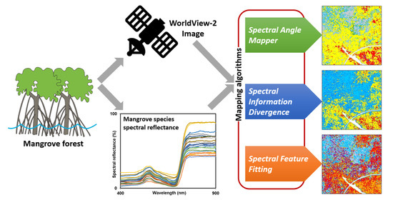
2. Materials and Methods

2.1. Study Site

The research area included Karimunjawa and Kemujan Island of Indonesia (5°49′33″–5°48′23″ S, 110°24′34″–110°28′37″ E). Their mangrove ecosystems comprise highly diverse mangrove species and are conservation areas in the Karimunjawa National Park, making them pristine and well-preserved. These two islands are located in the Karimunjawa District of Jepara Regency, Central Jawa Province, about 85 km north of Java Island (Figure 1). Several environmental factors that influence the growth of mangroves at the research site are the coastal physiography (topography), tides (length, duration, and range), waves and currents, climate (light, rainfall, temperature, and wind), salinity, dissolved oxygen, soil, and nutrients [10]. Based on the Schmidt and Ferguson climate classification, Karimunjawa and Kemujan Island have a C climate type with average rainfall of 3000 mm/year and air temperatures of 30–31 °C. Topographically, the Karimunjawa National Park area is located 0–506 m above sea level, spanning from flat coastal areas to undulating lowlands [11]. Hilly regions stretch from the east (highest peak) to the west and from the middle to the south. Karimunjawa experiences mixed tides with a prevailing diurnal pattern, i.e., one high and low tide but sometimes two high and low tides each day. The lowest low water level (LLWL) of the island waters is 20 cm, and the highest high-water level (HHWL) is 138 cm, making the maximum tidal range—the difference between the HHWL and LLWL—118 cm; this is classified as micro-tidal [12]. Karimunjawa and Kemujan Island have dark gray grumusol developed from quartz sandstone, micaceous sandstone, and quartz siltstone, and a few coral fragments included in mixed substrates (sand substrates and mixed gravels), with clay deposits along the coast. The soil physical properties on the two islands are fairly similar [11].
The Karimunjawa archipelago has five types of ecosystems: coral reefs, mangroves, seagrass beds, lowland tropical rainforests, and coastal forests. Mangrove ecosystems can be found on the coasts of Karimunjawa, Kemujan, Cemara Kecil, Cemara Besar, Krakal Kecil, Krakal Besar, Merican, Menyawakan, and Sintok Island, over a total area of 3.964 km2. There are 25 species (13 families) of true mangroves and nine species (seven families) of mangrove associates within the national park area, and five species (five families) of mangrove associates outside the national park [4]. Most of the mangroves on Karimunjawa and Kemujan Island are under the Karimunjawa National Park’s jurisdiction, and the community manages the rest. In general, the park consists of eight zones: core, wilderness, marine protection, marine tourism use, historical-cultural-religious use, rehabilitation, marine use, and traditional fisheries. The research sites are located in the wilderness and marine use zones. The mangrove area on Kemujan Island is used for trekking tours through the forest and bird watching towers.

2.2. Image Data and Processing

The primary data source in this study was the WorldView-2 (WV-2) image covering parts of Karimunjawa and Kemujan Island. It was acquired on 27 June 2020, with a 2 m spatial resolution (multispectral sensor) and eight multispectral bands as described in Table 1 [13]. The image was selected to match the acquisition time to the fieldwork that was conducted at the end of the rainy season and ensure a cloud-free image. In this study, image pre-processing was required to extract the spectral signatures of the targeted objects. The first part of image pre-processing was a radiometric correction to convert the image pixel value from digital numbers into at-sensor reflectance with Updike and Comp’s [14] procedure. The second part involved producing pixel values from the at-surface reflectance with fast line-of-sight atmospheric analysis of hypercubes (FLAASH) [15], an atmospheric correction model for the WV-2 image. The atmospheric visibility parameter was estimated from the moderate-resolution imaging spectroradiometer (MODIS) aerosol product [16].
Differences in the radiometric correction results at each level are visible in the object’s spectral reflectance curve (Z profile), presented in Figure 2. The spectral reflectance values in bands 1 (coastal) and 2 (blue) at the DN level (Figure 2a) decreased after correction at the surface reflectance level (Figure 2c), meaning that the atmospheric effects in the image had been corrected. The highest spectral reflectance values were in the red edge, near-IR1, and near-IR2 bands; in other words, the vegetation objects (mangroves) showed high reflectance values in these three bands. The spectral reflectance of mangroves forms a pattern similar to vegetation in general: low in the visible bands and high in the infrared bands (near-IR1 and near-IR2). This means that the radiometric and atmospheric corrections had been successfully applied to the WV-2 image.
The WV-2 image was visually interpreted to distinguish between mangrove and non-mangrove objects. True-color (RGB; 532) and false-color (near-IR1, red, blue; 752) composite images were used in this process, and mangrove and non-mangrove objects were identified based on their colors, tones, textures, and associations. The false-color composite image (752) depicts any vegetation features in red. However, it does not distinguish between mangroves and non-mangroves in areas formerly used as fish ponds. The true-color image composition was added to assist in this discrimination process. Mangrove objects can also be identified from their associations with surrounding objects, i.e., mangroves are located in coastal areas or border the sea. This mangrove object delineation output was then inputted for image masking to separate mangrove objects from others.

2.3. Field Data Collection

The spectral reflectance values of the targeted mangrove species were collected directly from the sampling points during 5–10 March 2021. The number and locations of field samples were selected purposively based on the Pixel Purity Index (PPI) values [17] and the sites’ accessibility. The PPI, in this case, was used to locate the purest mangrove pixels in the WV-2 image for spectral reflectance collection. The PPI image was produced from the minimum noise fraction (MNF) algorithm to remove the noise in the data and reduce the computational requirements for further processing. This research used 10,000 iterations because, according to Plaza and Chang [18], PPI produces pure pixels after 10,000 to 100,000 repetitions. These samples were then plotted onto a map that was later used to read the spectral reflectance of mangrove species in the field.
The field data collection resulted in 201 point samples covering 24 targeted mangrove species (Table 2). The distribution of the field samples is presented in Figure 1. The field samples were divided into two major groups: modeling samples for developing the spectral library (24 samples, Figure 3a) and validation models for the accuracy assessment of the resulting map (177 samples, Figure 3b). The modeling samples were spectral reflectance mangrove species collected in the areas with high species diversity. This research only focused on the true mangrove species, and researchers were assisted by park managers or rangers familiar with the targeted species’ location to collect these samples. The validation samples were mangrove species identified in the field. The validation sample locations were selected from “white pixels” (i.e., pure pixels) derived from the PPI calculation. In addition to PPI, the validation samples were also determined with aerial photos to identify a mix of two species (Avicennia marina and Ceriops tagal) found in the field.
The field spectral reflectance values of mangrove species were measured with a JAZ EL-350 portable spectrometer from Ocean Optics (https://oceanoptics.com/, accessed on 14 November 2021). First, the white and dark references were measured. A white reference produces a standard “white object” spectral reflectance reading to calculate the object’s spectral sample, while a dark reference produces a reading of an object with perfect absorption to create a “black body” reference [19]. Second, the spectral reflectance values of mangrove species were measured at the leaf level (Figure 3a), based on the criterion that healthy leaves appeared entirely green or contained chlorophyll.
Some important aspects to consider in collecting spectral reflectance data for mangrove species in the field are (1) the field of view (FOV) of the spectrometer sensor, (2) the distance between the spectrometer and the targeted object, (3) the angle and direction of measurement, and (4) the light conditions at the time of observation [19]. Kamal et al. [20] collected the spectral reflectance of Rhizophora stylosa on Karimunjawa Island at 2 cm, 50 cm, 1 m, 2 m, and 5 m distances with ten readings at each distance. According to this study, the spectral reflectance curves recorded at close range to the leaf (i.e., 2 cm) and from the furthest distance (i.e., 5 m) showed the lowest curve variation between readings. Therefore, this study used a distance of 2 cm for leaf spectral measurements to ensure that only the mangrove leaf was read (Figure 3a) and ensure highly consistent spectrometer results across readings [20,21]. The spectrometer’s measurement angle was set at 45° to the nadir and facing the sun to avoid shadows on the target object. In addition, the number of spectrometer reading repetitions affects the degree of confidence in the reading results. The leaf measurements were repeated six times to ensure the consistency of the readings in similar natural lighting conditions in the field.
The field-measured spectral reflectance profiles were stored in a file in .jaz format. A .jaz file contains reference spectrum data (white reflectance), dark reflectance, and the targeted object spectral reflectance data, which are used to construct the object’s spectral reflectance curve. The six replicates used to measure each mangrove species object avoided errors such as saturation in the spectral reflectance measurement, which increased the spectrometer readings’ precision. The field measurements produced data on objects’ light intensity at a particular wavelength; thus, the reflectance values needed to be calculated. These values were normalized and calculated with the formula described in Kamal et al. [19] and Wicaksono et al. [22]. The normalized and mean values were then used as input to build a spectral library.

2.4. Mangrove Species Clustering Analysis

White and dark reference readings were collected for each measurement of mangrove species samples using the spectrometer to normalize the spectral reflectance of each mangrove species and create a standard range of spectral reflectance values. This allows the derived spectral reflectance curves of different mangrove species to be compared directly. Mangrove species’ spectral reflectance can be analyzed effectively at wavelengths of 350–900 nm with a JAZ EL-350 spectrometer [20]. This wavelength range was selected because, based on the specifications of the spectrometer used, noise is likely to occur below 350 nm and above 900 nm. The mangrove species spectra compiled in the spectral library were then resampled according to the center wavelength of the WV-2 image bands and used to develop an optical dendrogram. An optical dendrogram determines how components (i.e., mangrove species) are grouped spectrally. It is also used to identify similarities and cluster distances between species or groups. The optical dendrogram for this study was created in the IBM SPSS Statistics 24 program based on Wicaksono et al.’s [22] work, which used seagrass as the research object and the Ward linkage method. The derived dendrogram was then used as the basis for the mangrove species classification scheme in remote sensing-based mapping.
The dendrogram was built using the Ward linkage method as described by Wicaksono et al. [22]. It analyzes clusters hierarchically by determining the distance between two clusters expressed as an increase in the “error sum of squares” (ESS). The Ward linkage method selects grouping steps sequentially to minimize the ESS at each step. The dendrogram was not developed from the field-measured spectral reflectance but rather the resampled data; therefore, eight wavelengths were selected to represent the eight WV-2 image bands. The resampled spectral reflectance values were inputted in the dendrogram for further use in pixel-based mapping. This dendrogram identifies similarities and cluster distances between mangrove species, producing several large groups according to the combination of cluster distances.

2.5. Pixel-Based Classification and Accuracy Assessment

The field-collected spectral samples were extracted and divided into three types: white reference, dark reference, and the object’s spectral reference. This extraction was performed to produce the spectral reflectance curves of mangrove species for a spectral library, i.e., a collection of references containing the spectral reflectance values of various objects [19,20]. A normalization process was conducted to obtain the appropriate spectral reflectance curves allowing for easy understanding and high representativeness. The extracted spectral reflectance samples of mangrove species were then collected in one container to be inputted into a spectral library in the ENVI 5.3 program. The compiled spectral library of mangrove species from field measurements was spectrally resampled to align with the spectral resolution of the WV-2 image as the basis of mangrove species mapping.
The mangrove species were mapped in ENVI 5.3 using the spectral library from the resampled spectra as the classification input or endmember. For this purpose, three pixel-based classification algorithms were applied and evaluated for mapping mangrove species, namely the spectral angle mapper (SAM), spectral information divergence (SID), and spectral feature fitting (SFF). The SAM algorithm can classify objects based on their spectral reflectance values by considering the illumination angle reflected by the object. SAM determines the similarity between two spectral reflectance objects by calculating the “spectral angle” created between them and treating them as vectors in a space with dimensionality equal to the number (n) of image bands used [23,24]. Because it only factors in the direction of the spectrum, the spectrum length and other factors are considered equal. It determines the similarity of the unknown spectrum t to the reference spectrum r using Equation (1), below:
α = c o s 1 ( t   ·   r | | t | |   | | r | | )
The SID algorithm can determine the target pixel based on differences in the object’s spectral reflectance information. It calculates the information difference between the target pixel (r1) and the target reference (r2) from the sum of the relative difference between r1 and r2 (D(r1r2)), and the relative difference between r2 and r1 (D(r2r1)). This algorithm is presented in Equation (2) below [25]:
SID ( r 1 , r 2 ) = ( D ( r 1 | | r 2 ) ) + ( D ( r 2 | | r 1 ) )
Finally, the SFF algorithm compares the spectral image with the endmember reference. The reference spectra were scaled to match those of the image after the continuum was removed from both datasets (reference and object spectra) [26].
The spectral reflectance of each mangrove species was measured in the field simultaneously with the validation samples. The validation samples are different datasets from those used to map the mangrove species. They contain mangrove species data and their coordinate locations in the field. However, both modeling and validation samples were determined with the same purposive sampling technique because of high object heterogeneity in the field and low accessibility. Both sets of samples were also selected with the same criteria, i.e., the PPI calculation results.
The accuracy assessment was conducted with a confusion matrix to measure the extent to which the mangrove species classification results from field-collected and post-field-processed data were similar. In addition to percent accuracy, it also evaluated each algorithm’s misclassification by observing the presence or absence of a logical error in the species classification. This accuracy assessment resulted in user’s accuracy (UA), producer’s accuracy (PA), and overall accuracy (OA) values, following Congalton and Green’s procedures [27].

3. Results

3.1. Spectral Reflectance of Mangrove Species

The spectral library for each species was developed by displaying the spectral reflectance curve of the replicated samples with their averages and observing the corresponding curves of all species. The normalized spectral reflectance of 24 mangrove species (10 of primary data and 14 of secondary data) were combined into one spectral reflectance curve, as shown in Figure 4a. The field-measured spectral reflectance has a very high spectral resolution (1586 bands) while that from the WV-2 image has a low resolution (eight bands). Therefore, spectral resampling was conducted to match the spectral resolution derived from the spectrometer to the WV-2 image bands. The center wavelengths of the WV-2 image obtained from the “Radiometric Use of WorldView-2 Imagery” guidelines by DigitalGlobe [13] were used as the targeted spectra in the spectral resampling process. The center wavelength for each WV-2 band is as follows: 427 nm (coastal), 478.3 nm (blue), 545.8 nm (green, 607.7 nm (yellow), 658.8 nm (red), 724.1 nm (red-edge), 832.9 nm (NIR1), and 949.3 nm (NIR2). Besides degrading spectral resolution, spectral resampling also simplified the spectral reflectance of objects measured in the field. In general, both field-collected and resampled data had the same pattern: low in the coastal, blue, and red bands, slightly high in the green band, high in the red-edge band, and very high in the near-IR1 and near-IR2 bands (Figure 4a,b).

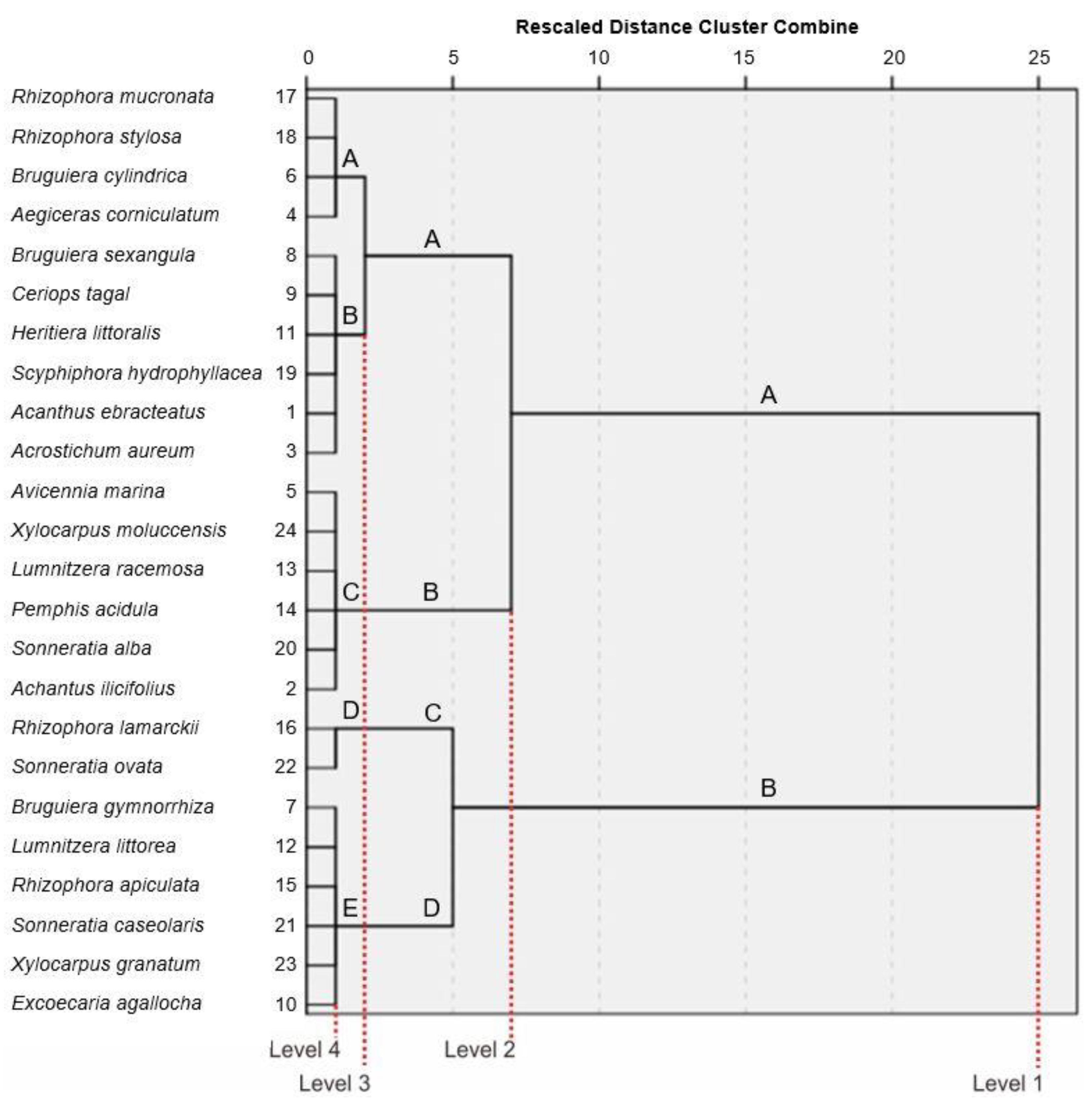
3.2. Clustering Analysis of Mangrove Species

The clustering of mangrove species was conducted based on the resampled mangrove spectra. Indirectly, this clustering also grouped several morphological features of plants, especially their leaves. Klančnik and Gaberščik [28] explained that every leaf shape has structural characteristics with distinctive optical properties. The redundancy analysis showed that the leaves’ morphological and biochemical characteristics had particular relationships with leaf spectral reflectance. In general, the most dominant plant part that can be identified by satellite imagery is the leaf canopy. In this study, the spectral reflectance approach used as input in the clustering analysis indirectly captured some of the morphological characteristics of the mangroves, especially the leaves.
Based on the resulting dendrogram (Figure 5), there were four possible classification schemes. The cluster distance for the most distinguishable class was 25, while the cluster distance for the least distinguishable class was 0. The dendrogram showed four levels with different numbers of species groups. Level 1 (two groups), Level 2 (four groups), and Level 3 (five groups) can be used as references in pixel-based mangrove species mapping because they have a relatively large distance between clusters (Table 3). Meanwhile, the Level-4 classification scheme cannot be used for this purpose because the distances between clusters are too small. The results of this species clustering are used to design scenarios for mangrove species mapping using the WV-2 image.

3.3. Pixel-Based Classification

The classification mapping was based on the dendrogram analysis results, which produced four levels of mangrove species groups. First, the spectral reflectance curves for each group of mangrove species at each level of the dendrogram were averaged. Then, these results were inputted into the three algorithms of mangrove species mapping. The SAM- and SID-based classifications used default thresholds of 0.1 and 0.05, respectively. Because there was no default threshold for the SFF, the threshold value was set at 10. For each dendrogram level, the threshold values of the classification algorithms were made equal to reduce user intervention and maximize software performance. The mapping results of using these three classification algorithms are presented in Figure 6. Overall, the SAM-based mangrove species classification results at Levels 1, 2, and 3 could not classify all mangrove areas, as was evident from the extensive gray areas in the mangrove delineation results. Some of the mangrove areas were unclassified; this could be due to an inappropriate threshold value for the classification. The front/distal formation bordering the seawater was generally dominated by Rhizophora groups and some Bruguiera individuals. The SAM algorithm found Pemphis acidula in the distal formation, but this species was not entirely classified in the Level-3 mapping. Meanwhile, the Level-1 mapping with the SID and SFF algorithms classified the distal formation as Group B with eight species, three of which were Bruguiera gymnorrhiza, Rhizophora lamarckii, and Rhizophora apiculata. According to field reports, Rhizophora groups and some Bruguiera individuals generally dominated the distal formation bordering the sea, meaning that Rhizophora apiculata is highly likely to have been among the species classified.
The Level-2 SID-based mapping showed Group A as the dominant species constituent. Group A consisted of several understory genera, such as Achantus, Acrosticum, Aegiceras, and Scyphiphora and some trees, such as Bruguiera sexangula, Bruguiera cylindrica, Ceriops tagal, Rhizophora mucronata, and Rhizophora stylosa, located in the medial and proximal formations. Meanwhile, the distal formation was dominated by Groups B and D, creating a mixed pattern. In contrast, the Level-2 SFF-based classification showed that the distal formation was dominated by Group C, consisting of Rhizophora lamarckii and Sporomusa ovata. However, these results were inaccurate as these two species cannot grow large and are rarely present in tidal areas but instead reside in the medial and the proximal areas. Meanwhile, the SID- and SFF-based classifications at Level 3 also showed significant differences in species composition; the former showed Group B predominating and the latter, codominant Groups A, C, and D.
The individual species mapping results (Level 4) differed from the other three classifications. The SAM and SID algorithms classified Pemphis acidula as the dominant species in the distal formation, although it is rarely found in tidal areas such as this distal formation, typically growing under the canopy of the proximal formation. This causes a visual classification error and subsequently affects the accuracy of the classification mapping using both algorithms. Meanwhile, SFF classified Bruguiera sexangula as the dominant species in the distal formation. It is commonly found in tidal areas and is associated with Rhizophora but not as a major species with broad distribution. The SFF-based classification suggested the presence of Bruguiera sexangular along the tidal area, another imprecise result that affects the mapping accuracy value.

4. Discussion

4.1. Mangrove Species Clusters

Mangrove species clustering can adopt plant morphological approaches commonly used in compiling taxonomies. For example, leaf shape, canopy shape, stem characteristics, and plant habitat characteristics such as salinity level, type of substrate, and length of tidal inundation can be used. However, the spectral reflectance curve of the mangrove species object on the WV-2 image was integrated with the field-measured curve for this study. The result of the spectral reflectance resampling was then inputted into the clustering in dendrograms for pixel-based mapping classification.
The results of the dendrogram analysis showed four levels with varying numbers of species groups (Figure 5 and Table 3). Level 1 (2 groups), Level 2 (4 groups), and Level 3 (5 groups) could be used as references for the pixel-based mapping of mangrove species because the clusters were quite far apart. In contrast, Level 4 could not be used for the same purpose because the clusters were too close together. The Level 1 scheme had a cluster distance of 25, resulting in two large clusters in which Bruguiera, Lumnitzera, Rhizophora, Sonneratia, and Xylocarpus were divided into two groups. In the Level 2 scheme with a cluster distance of 5, the mangrove species were divided into four groups. The species Rhizophora lamarckii and Sonneratia ovata were clustered into one group for the similarity of their spectral reflectance; physiologically, the two species also have more wax coating on the leaf surfaces compared with other species. The Level 3 scheme had a cluster distance of two, which divided the mangrove species into five groups where group A, at a rescaled distance of 5, was split into two new groups while the other three groups remained. Unlike in Levels 1–3, the Level 4 scheme grouped mangroves by single species, without forming new groups.

4.2. Accuracy Assessment of the Resulting Maps

The mapping accuracy was assessed with a confusion matrix to calculate the overall accuracy (OA), producer’s accuracy (PA), and user’s accuracy (UA). The validation samples were point data obtained directly from the field survey in 2021 (primary data) and secondary data with the attributes of mangrove species. The primary data were acquired using the average point method at 2 m × 2 m pure pixel points that had been created. Additionally, the samples were incidentally collected when encountering certain minor species that had gone unidentified during the interpretation of the aerial photographs. To assess the accuracy of the mapping results, a total of 177 sample points were analyzed using the “extract values to point” tool in ArcGIS on the model developed previously to compile the matrix.
In this step, the mangrove species maps generated using the three classification algorithms were evaluated for their OA, as presented in Table 4 and Table 5. In general, the accuracy of the three classification algorithms at all four levels was low. The SID-based classifications at Levels 1 (with two species groups), 2 (four), and 3 (five) had the highest OA at 49.72%, 22.60%, and 15.25%, respectively. Meanwhile, the SFF-based classification for the Level-4 mapping of 24 species had the highest OA at 5.08%. The results demonstrated that the greater the number of classes to be mapped, the smaller the accuracy value. This finding corresponds to Andréfouët et al. [29] and Kamal et al. [30], who explained that the percentage of classification accuracy expressed in OA decreased with the increase in the number of classes. In addition, the high heterogeneity of objects with natural properties, such as mangroves and mixed species in one pixel, affected the OA. The characteristics of mapped objects also affect the accuracy because if more pixels are mixed, the objects will be more difficult to classify.
The mapping accuracy assessment also calculated UA and PA for each classification algorithm and each dendrogram level to determine which errors reduced the accuracy. In general, the UA of all classification algorithms at each level was higher than the PA, as not all of the validation samples matched the classification model; many fell into a different class (unclassified or class “0”). With many samples considered unclassified, the PA decreased because, in contrast to UA, the number of correctly classified samples as the divisor increased. At Level 1 classifications with the SAM, SID, and SFF algorithms, there were, respectively, 148, 26, and 43 unclassified points among 177 samples. Furthermore, the SAM, SID, and SFF-based classifications led to 137, 24, and 38 unclassified points at Level 2; 132, 15, and 27 unclassified points at Level 3; and 63, 5, and 13 unclassified points at Level 4. The SAM-based classification had the highest number of unclassified points at all levels, resulting in low PA, UA, and OA.
The SAM algorithm demonstrated the lowest accuracy at all levels because the default threshold of 0.1 was used, leaving the mangrove area partially unclassified. The accuracy points extracted from the SAM model did not overlap because the mangrove area was not classified. The number of unclassified points significantly affected the accuracy of the SAM-based mapping results. Not all accuracy points that overlap with the model show accurate or desirable results. At Levels 1, 2, and 3, the points that did not overlap in the class that should have been the majority were placed in the last class, namely classes B, D, and E, respectively. At Level 4, the inaccurate points were mostly classified as Pemphis acidula and Sonneratia caseolaris. These issues significantly decreased the OA of SAM-based classification.
Mapping single species with the SID- and SFF-based classifications resulted in overlapping classes with more accuracy points than using SAM. The accuracy points in the SID-based classification overlapped more with Acrostichum aureum, Aegiceras corniculatum, Pemphis acidula, and Sonneratia caseolaris than with other species. Meanwhile, in the SFF-based classification, the accuracy points overlapped more with Aegiceras corniculatum, Bruguiera sexangula, and Pemphis acidula. However, according to the classification results, there were only nine overlapped accuracy points with the correct values when using the SFF and none when using the SID. In pixel-based mapping, increasing the classes to be mapped will reduce the accuracy value. In contrast, Kamal et al. [30] mapped Rhizophora stylosa and produced an OA of 52%. Hirano et al. [31] conducted a similar study mapping Rhizophora mangle that resulted in an OA of 40%. Mixed pixels are one of the problems that arise in remote sensing images because one pixel in the image can consist of two or more types of objects. Likewise, mixed pixels were common in the WV-2 satellite imagery used in this study because of the high heterogeneity and species diversity of the area. Hyperspectral field data used as the input in multispectral images also affects the mapping accuracy. Ideally, this type of study should be based on hyperspectral image data so the spectral resolution would be similar.

4.3. Classification Performance Evaluation

The three classification algorithms have different characteristics, each with particular advantages and disadvantages. They have dissimilar capacities in recognizing objects even from the same type of data source, i.e., the field-measured spectral reflectance of mangrove species. In the SAM algorithm, the similarity between the two spectra is determined by calculating the “spectral angle” between the image spectrum and the object spectrum and then assuming a vector in the same dimensional space with the same number of bands [32]. Its disadvantages include insensitivity to other known factors (besides angle) and using the same treatment for all illumination because SAM only uses spectrum “direction” and not spectrum “length.” SAM only considers the spectral reflectance pattern of the object, not the difference in the intensity of the object’s spectral reflectance [33]. The SAM-based classification uses vector directions to distinguish between features’ spectral reflectance properties. Features with smaller spectral angles are categorized into the same class. SAM classifies pure classes and leaves the rest unclassified, thus failing to classify entire plant species with pure pixels in the mangrove area [32,34]. In addition, the factors considered in determining the threshold value affect the classification results, especially at Levels 1, 2, and 3.
In contrast to SAM, the SID algorithm considers each pixel a random variable, using a spectral histogram to obtain a mapped probability. Muhammad and Mirza [34] suggest that problems arising from the SAM classification algorithm can be minimized by using SID. SID was applied to the same endmember to classify unclassified species and impure pixels in SAM-based classification results. The SID algorithm uses the size of the divergence to match pixels to spectral references. A smaller divergence means that the pixel is more likely to be similar to the spectral reference. According to Nidamanuri and Zbell [35], SID-based classification can measure the spectral variability of a single mixed pixel and determine similar spectra. However, according to Shanmugam and Srinivasaperumal [36], SID’s weakness is that it is more effective on mixed pixel targets.
The SFF classification algorithm produces a separate scale image and root mean square (RMS) image or a combination of both. SFF is an absorption feature-based algorithm that matches the image spectrum (pixels) with the object spectrum (reference) [37]. In this study, SFF classified areas of high species diversity better than SAM and SID in single species mapping (Level 4). However, according to Muhammad and Mirza [34], this algorithm is the most time-consuming to use and the resulting classification still needs improvements. For the input, SFF requires a reference spectrum of the image or spectral library. The second requirement is removing the continuum from the image and spectral reference (object) before analysis [37], for instance, by resampling that degrades the spectral resolution of the data to that of the image.

5. Conclusions

This study identified 24 mangrove species on Karimunjawa and Kemujan Island. Based on their spectral reflectance characteristics, there were four dendrogram levels: Level 1 (consisting of two groups), 2 (four groups), 3 (five groups), and 4 (single species). The SAM-based classifications at Levels 1, 2, and 3 did not entirely classify the mangroves. The SAM and SID algorithms successfully mapped Pemphis acidula massively in the distal formation at Level 4. Using SID, Group B was found to prevail at Level 1 while Group A was dominant at Level 2. At the same level, the SFF algorithm classified Group C as dominant in the distal formation (Rhizophora lamarckii and Sonneratia ovata). Meanwhile, the SID- and SFF-based classifications at Level 3 showed Group B prevailing in the former and codominant Groups A, C, and D in the latter. The SFF algorithm classified Bruguiera sexangula in the distal formation. The best accuracy for mapping mangrove species distribution was obtained by applying the SID-based classification at Levels 1, 2, and 3, with overall accuracies of 49.72%, 22.60%, and 15.20%, respectively. Meanwhile, the best single-species mapping accuracy (Level 4) was obtained with SFF-based classification, with an overall accuracy of 5.08%. In conclusion, the three classification algorithms offered low mapping accuracy due to the high heterogeneity of species in the field, which resulted in many mixed pixels and limited access to obtain evenly distributed accuracy points. The greater the number of classes to be mapped, the smaller the accuracy. A predefined threshold value that is less than optimal is also a source of low accuracy. Future research can focus on assessing whether the number of mangrove species affects the accuracy of mapping results. This can be achieved by replicating the mapping method in a mangrove environment with low species variation.

Author Contributions

Conceptualization and methodology, A.D.R., M.K. and P.W.; validation and formal analysis, A.D.R.; writing—original draft preparation, A.D.R.; writing—review and editing, M.K and P.W.; visualization, A.D.R.; supervision, M.K. and P.W.; funding acquisition, M.K. All authors have read and agreed to the published version of the manuscript.

Funding

This research was funded by the 2021 Penelitian Terapan Unggulan Perguruan Tinggi Grant scheme provided by the Ministry of Education, Culture, Research and Technology of the Republic of Indonesia (contract number 1738/UN1/DITLIT/DIT-LIT/PT/2021).

Institutional Review Board Statement

Not applicable.

Informed Consent Statement

Not applicable.

Data Availability Statement

The data presented in this study are available from the first author on request.

Acknowledgments

The authors would like to thank (1) the Department of Geographic Information Science at the Faculty of Geography, Universitas Gadjah Mada, for providing research facilities and equipment, (2) the Karimunjawa National Park management for granting fieldwork permits, and (3) S.M. Ridha and M.S. Usni for their invaluable assistance during the fieldwork.

Conflicts of Interest

The authors declare no conflict of interest. The funders had no role in the design of the study; the collection, analysis, or interpretation of data; the writing of the manuscript; or the decision to publish the results.

References

  1. Bunting, P.; Rosenqvist, A.; Lucas, R.M.; Rebelo, L.-M.; Hilarides, L.; Thomas, N.; Hardy, A.; Itoh, T.; Shimada, M.; Finlayson, C.M. The Global Mangrove Watch—A New 2010 Global Baseline of Mangrove Extent. Remote Sens. 2018, 10, 1669. [Google Scholar] [CrossRef] [Green Version]
  2. Kusmana, C. Distribution and Current Status of Mangrove Forests in Indonesia. In Mangrove Ecosystems of Asia: Status, Challenges and Management Strategies; Faridah-Hanum, I., Latiff, A., Hakeem, K.R., Ozturk, M., Eds.; Springer: New York, NY, USA, 2014; pp. 37–60. [Google Scholar] [CrossRef]
  3. Spalding, M.; Kainuma, M.; Collins, L. World Atlas of Mangroves; Earthscan: London, UK, 2010. [Google Scholar]
  4. Karimunjawa National Park. Jenis Mangrove Taman Nasional Karimunjawa [Mangrove Species in the Karimunjawa National Park]; Karimunjawa National Park: Semarang, Indonesia, 2012. (In Indonesian) [Google Scholar]
  5. Ilman, M.; Dargusch, P.; Dart, P. A historical analysis of the drivers of loss and degradation of Indonesia’s mangroves. Land Use Policy 2016, 54, 448–459. [Google Scholar] [CrossRef]
  6. Lewis, D.; Phinn, S.; Arroyo, L. Cost-effectiveness of seven approaches to map vegetation communities—A case study from Northern Australia’s tropical savannas. Remote Sens. 2013, 5, 377–414. [Google Scholar] [CrossRef] [Green Version]
  7. Kuenzer, C.; Bluemel, A.; Gebhardt, S.; Quoc, T.V.; Dech, S. Remote sensing of mangrove ecosystems: A review. Remote Sens. 2011, 3, 878–928. [Google Scholar] [CrossRef] [Green Version]
  8. Lucas, R.; Lule, A.V.; Rodríguez, M.T.; Kamal, M.; Thomas, N.; Asbridge, E.; Kuenzer, C. Spatial Ecology of Mangrove Forests: A Remote Sensing Perspective. In Mangrove Ecosystems: A Global Biogeographic Perspective: Structure, Function, and Services; Rivera-Monroy, V.H., Lee, S.Y., Kristensen, E., Twilley, R.R., Eds.; Springer: Cham, Switzerland, 2017; pp. 87–112. [Google Scholar]
  9. Vaiphasa, C.; Ongsomwang, S.; Vaiphasa, T.; Skidmore, A.K. Tropical mangrove species discrimination using hyperspectral data: A laboratory study. Estuar. Coast Shelf Sci. 2005, 65, 371–379. [Google Scholar] [CrossRef]
  10. Alwidakdo, A.; Azham, Z.; Kamarubayana, L. Studi Pertumbuhan Mangrove Pada Kegiatan Rehabilitasi Hutan Mangrove. Agrifor Jurnal Ilmu Pertanian dan Kehutanan 2014, 13, 11–18. (In Indonesian) [Google Scholar]
  11. Department of Forestry. Buku Informasi 50 Taman Nasional di Indonesia. In Book of Information on 50 National Parks in Indonesia; Directorate General of Forest Protection and Nature Conservation: Jakarta, Indonesia, 2007. (In Indonesian) [Google Scholar]
  12. Musa, M.; Handoyo, G.; Setyono, H. Peramalan Pasang di Perairan Pulau Karimunjawa, Kabupaten Jepara, Menggunakan Program “Worldtides”. J. Oceanogr. 2013, 3, 1–7. (In Indonesian) [Google Scholar]
  13. Data Sheet WorldView-2. Available online: https://dg-cms-uploads-production.s3.amazonaws.com/uploads/document/file/98/WorldView2-DS-WV2-rev2.pdf (accessed on 1 October 2016).
  14. Updike, T.; Comp, C. Radiometric Use of WorldView-2 Imagery. Available online: https://www.digitalglobe.com/sites/default/files/Radiometric_Use_of_WorldView-2_Imagery%20%281%29.pdf (accessed on 1 August 2013).
  15. Matthew, M.W.; Adler-Golden, S.M.; Berk, A.; Richtsmeier, S.C.; Levine, R.Y.; Bernstein, L.S.; Acharya, P.K.; Anderson, G.P.; Felde, G.W.; Hoke, M.P.; et al. Status of Atmospheric Correction Using a MODTRAN4-Based Algorithm. In Proceedings of the SPIE 4049 Algorithms for Multispectral, Hyperspectral, and Ultraspectral Imagery VI, Orlando, FL, USA, 23 August 2000. [Google Scholar]
  16. Level 1 and Atmosphere Archive and Distribution System (LAADS) DAAC. Available online: https://earthdata.nasa.gov/eosdis/daacs/laads (accessed on 15 December 2020).
  17. Boardman, J.W. Automated Spectral Unmixing of AVIRIS Data using Convex Geometry Concepts. In Proceedings of the Summaries of the 4th Annual JPL Air-Borne Geosciences Workshop, Pasadena, CA, USA, 25 October 1993; pp. 11–14. [Google Scholar]
  18. Plaza, A.J.; Chang, C.I. High Performance Computing in Remote Sensing; Chapman and Hall/CRC: Boca Raton, FL, USA, 2008. [Google Scholar]
  19. Kamal, M.; Arjasakusuma, S.; Adi, N.S. JAZ EL-350 VIS NIR Portable Spectrometer Operational Guideline; Remote Sensing Laboratory, Faculty of Geography Universitas Gadjah Mada: Yogyakarta, Indonesia, 2012. [Google Scholar]
  20. Kamal, M.; Ningam, M.U.L.; Alqorina, F. The Effect of Field Spectral Reflectance Measurement Distance to the Spectral Reflectance of Rhizophora stylosa. In Proceedings of the IOP Conference Series: Earth and Environmental Science, Yogyakarta, Indonesia, 27–28 September 2017; Volume 98. [Google Scholar]
  21. Kamal, M.; Ningam, M.U.L.; Alqorina, F.; Wicaksono, P.; Murti, S.H. Combining field and image spectral reflectance for mangrove species identification and mapping using WorldView-2 image. In Proceedings of the SPIE Remote Sensing 10790, Earth Resources and Environmental Remote Sensing/GIS Applications IX, 107901P, Berlin, Germany, 9 October 2018. [Google Scholar]
  22. Wicaksono, P.; Fauzan, M.A.; Kumara, I.S.W.; Yogyantoro, R.N.; Lazuardi, W.; Zhafarina, Z. Analysis of reflectance spectra of tropical seagrass species and their value for mapping using multispectral satellite images. Int. J. Remote Sens. 2019, 40, 8955–8978. [Google Scholar] [CrossRef]
  23. Kruse, F.A.; Lefkoff, A.B.; Boardman, J.W.; Heidebrecht, K.B.; Shapiro, A.T.; Barloon, P.J.; Goetz, A.F.H. The Spectral Image Processing System (SIPS)—Interactive Visualization and Analysis of Imaging Spectrometer Data. Remote Sens. Environ. 1993, 44, 145–163. [Google Scholar] [CrossRef]
  24. Borengasser, M.; Hungate, W.S.; Watkins, R. Hyperspectral Remote Sensing: Principles and Applications; Taylor & Francis in Remote Sensing Applications, CRC Press: New York, NY, USA, 2008. [Google Scholar]
  25. Chang, C.I. An Information-Theoretic Approach to Spectral Variability, Similarity, and Discrimination for Hyperspectral Image Analysis. IEEE Tras. Inf. Theory 2000, 46, 1927–1932. [Google Scholar] [CrossRef] [Green Version]
  26. Clark, R.N.; Swayze, G.A.; Gallagher, A.; Gorelick, N.; Kruse, F.A. Mapping with imaging spectrometer data using the complete band shape least-squares algorithm simultaneously fit to multiple spectral features from multiple materials. In Proceedings of the 3rd Airborne Visible/Infrared Imaging Spectrometer (AVIRIS) Workshop; JPL Publication 91-28; Jet Propulsion Laboratory: Pasadena, CA, USA, 20–21 May 1991; pp. 2–3. [Google Scholar]
  27. Congalton, R.G.; Green, K. Assessing the Accuracy of Remotely Sensed Data: Principles and Practices, 2nd ed.; CRC Press: Boca Raton, FL, USA, 2009. [Google Scholar]
  28. Klančnik, K.; Gaberščik, A. Leaf spectral signatures differ in plant species colonizing habitats along a hydrological gradient. J. Plant Ecol. 2016, 9, 442–450. [Google Scholar] [CrossRef]
  29. Andréfouët, S.; Kramer, P.; Torres-Pulliza, D.; Joyce, K.E.; Hochberg, E.J.; Garza-Pérez, R.; Muller-Karger, F.E. Multi-site evaluation of IKONOS data for classification of tropical coral reef environments. Remote Sens. Environ. 2003, 88, 128–143. [Google Scholar] [CrossRef]
  30. Kamal, M.; Phinn, S.; Johansen, K. Object-Based Approach for Multi-Scale Mangrove Composition Mapping Using Multi-Resolution Image Datasets. Remote Sens. 2015, 7, 4753–4783. [Google Scholar] [CrossRef] [Green Version]
  31. Hirano, A.; Madden, M.; Welch, R. Hyperspectral image data for mapping wetland vegetation. Wetland 2003, 23, 436–448. [Google Scholar] [CrossRef]
  32. Rashmi, S.; Addamani, S.; Venkat, S. Spectral Angle Mapper Algorithm for Seagrass and Other Benthic Habitats in Bolinao, Pangasinan using Worldview-2 Satellite Image. In Proceedings of the Geoscience and Remote Sensing Symposium (IGARSS): IEEE International, Melbourne, Australia, 21–26 July 2013; pp. 1579–1582. [Google Scholar] [CrossRef]
  33. Rahmandhana, A.D. Pemetaan Distribusi Jenis Mangrove Melalui Integrasi Citra WorldView-2 dan Pengukuran Spektrometer Lapangan di Pulau Karimunjawa dan Kemujan, Kabupaten Jepara [Mapping the Distribution of Mangrove Species through the Integration of WorldView-2 Image and Field Spectrometer Measurements in Karimunjawa and Kemujan Island, Jepara Regency]. Master’s Thesis, Universitas Gadjah Mada, Yogyakarta, Indonesia, 14 September 2021. (In Indonesian). [Google Scholar]
  34. Muhammad, S.; Mirza, M.W. Hyperspectral Mapping Methods for Differentiating Mangrove Species along Karachi Coast. Int. J. Environ. Ecol. Eng. 2013, 7, 963–965. [Google Scholar] [CrossRef]
  35. Nidamanuri, R.R.; Zbell, B. A method for selecting optimal spectral resolution and comparison metric for material mapping by spectral library search. Prog. Phys. Geog. 2010, 34, 47–58. [Google Scholar] [CrossRef]
  36. Shanmugam, S.; Srinivasaperumal, P. Spectral Matching Approaches in Hyperspectral Image Processing. Int. J. Remote Sens. 2014, 35, 8217–8251. [Google Scholar] [CrossRef]
  37. Hyperspectral Analytics in ENVI Target Detection and Spectral Mapping Methods. Available online: http://www.spectroexpo.com/wp-content/uploads/2021/03/Hyperspectral_Whitepaper.pdf (accessed on 10 December 2020).
Figure 1. Study area map—The Karimunjawa and Kemujan Islands displayed on a Landsat 8 OLI color composite image with RGB 546 band combination.
Remotesensing 14 00183 g001
Figure 2. Spectral reflectance curves of mangrove objects at three correction levels: (a) digital number, (b) at-sensor radiance, and (c) at-surface reflectance.
Remotesensing 14 00183 g002
Figure 3. Field data collection: (a) spectral reflectance measurement of the targeted mangrove species and (b) field validation sample collection.
Remotesensing 14 00183 g003
Figure 4. Spectral reflectance curves of the field-measured data (a) and the resampling results based on WorldView-2 bands (b) for the 24 mangrove species found in the study site.
Remotesensing 14 00183 g004
Figure 5. Dendrogram of mangrove species obtained with the Ward linkage method showing four levels of species grouping.
Remotesensing 14 00183 g005
Figure 6. Mangrove species mapping results using the SAM, SID, and SFF algorithms at group Levels 1–4.
Remotesensing 14 00183 g006
Table 1. Band characteristics of WorldView-2 imagery [13].
Spectral BandWavelengthSpatial Resolution
Panchromatic450–800 nm0.46 m
Multispectral–Coastal400–450 nm1.84 m
Multispectral–Blue450–510 nm1.84 m
Multispectral–Green510–580 nm1.84 m
Multispectral–Yellow585–625 nm1.84 m
Multispectral–Red630–690 nm1.84 m
Multispectral–Red Edge705–745 nm1.84 m
Multispectral–Near-IR1770–895 nm1.84 m
Multispectral–Near-IR2860–1040 nm1.84 m
Table 2. Mangrove species identified in the field survey.
NoMangrove SpeciesNoMangrove SpeciesNoMangrove Species
1Acanthus ebracteatus9Ceriops tagal17Rhizophora mucronata
2Acanthus ilicifolius10Excoecaria agallocha18Rhizophora stylosa
3Acrostichum aureum11Heritiera littoralis19Scyphiphora hydrophyllacea
4Aegiceras corniculatum12Lumnitzera littorea20Sonneratia alba
5Avicennia marina13Lumnitzera racemosa21Sonneratia caseolaris
6Bruguiera cylindrica14Pemphis acidula22Sonneratia ovata
7Bruguiera gymnorrhiza15Rhizophora apiculata23Xylocarpus granatum
8Bruguiera sexangula16Rhizophora lamarckii24Xylocarpus moluccensis
Table 3. Mangrove species grouping of Levels 1–4 resulting from the cluster analysis.
LevelGroupMangrove Species
Level 1AA. ebracteatus, A. ilicifolius, A. aureum, A. corniculatum, A. marina, B. cylindrica, B. sexangular, C. tagal, H. littoralis, L. racemosa, P. acidula, R. mucronata, R. stylosa, S. hydrophyllacea, S. alba, X. moluccensis
BB. gymnorrhiza, E. agallocha, L. littorea, R. apiculata, R. lamarckii, S. caseolaris, S. ovata, X. granatum
Level 2AA. ebracteatus, A. aureum, A. corniculatum, B. cylindrica, B. sexangular, C. tagal, H. littoralis, R. mucronata, R. stylosa, S. hydrophyllacea
BA. ilicifolius, A. marina, L. racemosa, P. acidula, S. alba, X. moluccensis
CR. lamarckii, S. ovata
DB. gymnorrhiza, E. agallocha, L. littorea, R. apiculata, S. caseolaris, X. granatum
Level 3AA. corniculatum, B. cylindrica, R. mucronata, R. stylosa
BA. ebracteatus, A. aureum, B. sexangula, C. tagal, H. littoralis, S. hydrophyllacea
CA. ilicifolius, A. marina, L. racemosa, P. acidula, S. alba, X. moluccensis
DR. lamarckii, S. ovata
EB. gymnorrhiza, E. agallocha, L. littorea, R. apiculata, S. caseolaris, X. granatum
Level 4 Individual mangrove species
Table 4. Accuracy of mangrove species mapping with SAM, SID, and SFF-based classifications at Levels 1, 2, and 3.
Classification AlgorithmsLevel 1 (%)Level 2 (%)Level 3 (%)
GroupPAUAOAGroupPAUAOAGroupPAUAOA
SAMA8.4047.627.34A5.8850.005.08A3.3325.005.65
B5.1737.50 B5.8815.00 B13.1633.33
C0.000.00 C5.8821.43
D3.8516.67 D0.000.00
E1.928.33
SIDA58.8266.6749.72A36.7631.2522.60A13.335.9715.25
B31.0339.13 B3.927.14 B42.1127.59
C0.000.00 C1.965.26
D25.0030.23 D0.000.00
E11.5435.29
SFFA21.8570.2738.42A10.2931.8210.73A6.674.657.91
B72.4143.30 B5.887.50 B5.2650.00
C50.000.00 C5.887.89
D11.5420.69 D50.006.25
E7.6923.53
Table 5. Accuracy of mangrove species mapping with SAM, SID, and SFF-based classifications at Level 4.
ClassSAMSIDSFF
PA (%)UA (%)OA (%)PA (%)UA (%)OA (%)PA (%)UA (%)OA (%)
A000.56000005.08
B000000
C000000
D000000
E000000
F000000
G000000
H000033.332.27
I000000
J00006.259.09
K000000
L000046.1537.50
M000000
N000000
O000000
P000000
Q000000
R000000
S000000
T000000
U33.332.440033.3316.67
V000000
W000000
X000000
Publisher’s Note: MDPI stays neutral with regard to jurisdictional claims in published maps and institutional affiliations.

