
Improved Active Deep Learning for Semi-Supervised Classification of Hyperspectral Image


1
School of Measurement-Control and Communication Engineering, Harbin University of Science and Technology, Harbin 150080, China
2
School of Electronics and Information Engineering, Harbin Institute of Technology, Harbin 150001, China
*
Author to whom correspondence should be addressed.
Remote Sens. 2022, 14(1), 171; https://doi.org/10.3390/rs14010171
Submission received: 1 December 2021
/
Revised: 28 December 2021
/
Accepted: 29 December 2021
/
Published: 31 December 2021
(This article belongs to the Special Issue Object-Level Remote Sensing Image Information Extraction and Applications)
Abstract
:Hyperspectral image (HSI) data classification often faces the problem of the scarcity of labeled samples, which is considered to be one of the major challenges in the field of remote sensing. Although active deep networks have been successfully applied in semi-supervised classification tasks to address this problem, their performance inevitably meets the bottleneck due to the limitation of labeling cost. To address the aforementioned issue, this paper proposes a semi-supervised classification method for hyperspectral images that improves active deep learning. Specifically, the proposed model introduces the random multi-graph algorithm and replaces the expert mark in active learning with the anchor graph algorithm, which can label a considerable amount of unlabeled data precisely and automatically. In this way, a large number of pseudo-labeling samples would be added to the training subsets such that the model could be fine-tuned and the generalization performance could be improved without extra efforts for data manual labeling. Experiments based on three standard HSIs demonstrate that the proposed model can get better performance than other conventional methods, and they also outperform other studied algorithms in the case of a small training set.
1. Introduction
In the past decades, satellite remote sensing has provided advanced detection and research tools for studying the Earth’s resources, for monitoring local and regional environmental changes, and for exploring global environmental changes, given its macroscopic, comprehensive, rapid, dynamic, and accurate measurements [1]. Hyperspectral images (HSIs) can simultaneously obtain the two-dimensional spatial image information and the three-dimensional spectral curve information of the ground material, which reflects the characteristics and advantages of the “map integration” [2,3]. Hyperspectral images are being increasingly used in many applications containing the field of fine recognition in agriculture [4] and building target detection or recognition in cities [5,6]. All these applications require ground class labels for each hyperspectral pixel vector. Due to this, HSI classification, as a fundamental and challenging task in hyperspectral remote sensing, has recently attracted considerable attention from remote sensing-oriented researchers [7].
HSI classification is the process of assigning a unique tag to each pixel vector to be uniquely represented by a certain class of the spectral and spatial characteristics of the image via a certain discriminant function. As methods for the feature extraction of hyperspectral data are being continuously improved, traditional classification methods, based on spectral features alone [8,9], no longer meet requirements for high classification accuracy. As a result, numerous scholars have successfully incorporated spatial information into classification and have proven the ability to improve the classification performance [10,11,12]. However, spatial-spectral features are commonly used as classification in only two ways: first, one can extract spectral and spatial features separately and input their stacked joint features into the classifier for classification; second, joint spatial-spectral features can be extracted simultaneously for classification.
The method for step-wise extraction of spectral and spatial features (for stacking them into classification) can effectively use spatial information as an input to achieve higher accuracy classification of ground features. In particular, Li et al. [13] proposed the application of the recent regularized subspace of Gabor filtering to hyperspectral image data classification, using two-dimensional Gabor filtering to extract spatial features in image regions. With the emergence of machine learning approaches, deep learning has been widely applied for HSI classification. The methods of simultaneous extraction of joint spatial-spectral features are becoming increasingly popular and include stacked auto-encoders [14], deep confidence networks [15] and convolutional neural networks (CNN) [16,17,18]. However, the classification through deep learning models requires a large number of labeled samples to train the classification model, but it suffers from the learning-related deficiency when labeled samples are limited. Moreover, these labeled samples not only require experts’ prior knowledge for labeling, but are also time-consuming, costly, and difficult to obtain in practice.
To alleviate the problem of poor learning effect when samples are limited, active learning (AL) methods with high labeling efficiency [19] were proposed. They have already been successfully applied to HSI classification. The main idea of AL is to artificially label a few unknown samples, by means of human-computer interaction, and expand the training set [20]. A new hyperspectral image data classification method with semi-supervised active learning has been proposed by previous studies [21,22], which took advantage of AL to increase training samples and improved the machine generalization performance. Although adoption of AL methods can improve the computational efficiency and classification accuracy, AL is a cyclical process of human-computer interaction. This implies the corresponding costs for human experts labeling samples and related time consumption.
Given the considerations above, we propose to add the idea of AL to the structure of deep learning. In this way, the random multi-graphs semi-supervised algorithm [23] can be utilized [23] to label unlabeled samples, thereby reducing the cost for human experts to label samples. The HSI classification algorithm, proposed in this study, can be summarized as follows. First, a finite dataset of labeled samples initializes the convolutional neural network and performs category probability prediction on the unlabeled sample set. This step is performed on the category probability output from the model, whereas the most informative samples are queried using AL strategy. Second, a random multi-graphs algorithm is introduced to label the unlabeled samples. In this way, one searches for pseudo-labels, corresponding to the informative samples in the pseudo-label candidate pool. Third, newly labeled samples are added to the training set to continuously fine-tune the CNN model until the stopping condition is satisfied.
The new method aimed to improve the generalization ability of the machine by using pseudo-labeled samples, which include robust and informative samples, automatically and actively selected through semi-supervised learning. In this way, the cost problem of manual labeling in traditional active learning is alleviated, thereby providing an efficient “self-learning process of the machine”.
The rest of this paper is organized as follows. Section 2 provides the related introduction of state-of-the-art HSI classification. An improved semi-supervised classification framework for active deep learning is proposed in Section 3. Section 4 evaluates the performance of the proposed approach on different datasets. Section 5 is the summary.
2. Related Work
2.1. Active Deep Learning Methods
Deep learning and active learning methods for the HSI classification have been extensively studied in the recent years. For instance, a previous study [24] introduced a convolutional neural network model with Markov random field in a Bayesian framework for HSI classification, which effectively exploits the spatial information of hyperspectral images. The previous scholars [25] proposed an improved spectral spatial deep convolutional neural network with 3D patch input. The AL query function, reported by [26], is based on a tree-integrated classifier that combines sample uncertainty and diversity criteria to select regions of interest for classification studies. Furthermore, spatial and spectral information has been used to solve problems in different remote sensing contexts [27], which improved the learning process of high-resolution remote sensing images.
Additionally, some scholars have successfully applied AL and deep learning in HSI classification [28,29,30]. More specifically, Liu et al. [28] proposed an active learning algorithm based on weighted incremental dictionary learning. Haunt et al. [29] introduced an AL-guided classification model by using spectral and spatial context information from hyperspectral data in a New Bayesian CNN. Furthermore, Cao et al. [30] have suggested that high classification accuracy, of different landmarks in hyperspectral images, can be achieved by applying the powerful feature extraction capability of CNNs, as well as the effective labeling efficiency of AL.
Although the active deep learning framework has effectively solved the problem of the scarcity of labeled samples in practical classification tasks, the samples were still manually labeled to realize the use of unlabeled samples in this model. Therefore, in view of the above issue, this paper considers utilizing a certain machine learning algorithm to replace human experts to label unlabeled samples, as well as combining with active learning query strategies, to establish an improved active deep semi-supervised classification model.
2.2. Random Multi-Graphs Algorithm
One of the challenges for the high-dimensional characteristics of hyperspectral remote sensing data is that HSI classification has to face the so-called Hughes phenomenon [31]. A new semi-supervised framework has been proposed to cope with high-dimensional and large-scale data, which combined the randomness with anchor graphs [32]. The advantages of random forest [33] include not over-fitting due to randomness and featuring good generalization performance. Moreover, the advantage of the anchor graph algorithm [34] is that it can linearly scale the size of the dataset, which is very suitable for HSI characteristics. This idea led to the introduction of a semi-supervised classification framework of HSI, based on random multi-graphs [23]. A graph was constructed in a randomly selected feature space by using an anchor graph method, whereas the semi-supervised inference was performed on the graph.
Although all these methods provide better results, they all have their own advantages and disadvantages in processing HSI classification. When active deep learning methods are used for HSI classification, the cost of labeling by human experts is yet inevitable and imposes the corresponding burden. Therefore, this study combined the random multi-graph algorithm to label a large number of the unlabeled samples using the spectral spatial features of a limited label samples. The AL idea was then used to select informative samples to join the training of CNN and continuously fine-tune the classification model. In this way, our study benefitted from both the random forest and anchor graph algorithms for processing large amounts of high-dimensional data and allowed combining the powerful feature extraction capability of deep learning with AL methods.
3. The Proposed Method
3.1. The Proposed Model
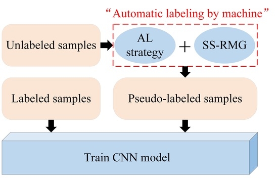
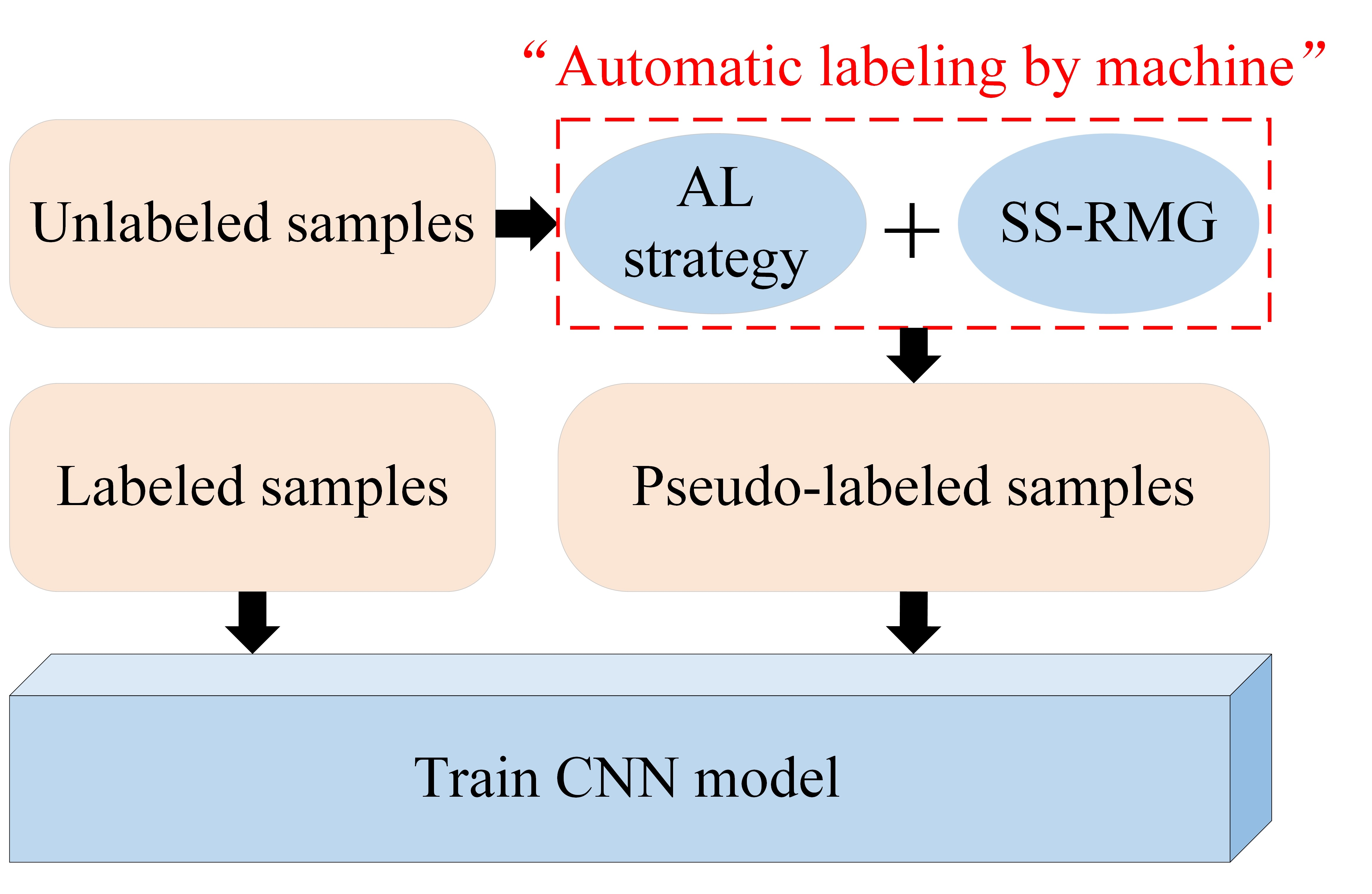
Figure 1 shows the framework of the proposed classification method in this paper. As seen, this framework combines active deep learning (ADL) and random multi-graphs algorithm by completely removing the action of human experts in active learning. It also combines self-learning and CNN iteration ideas to continuously fine-tune the classification model.
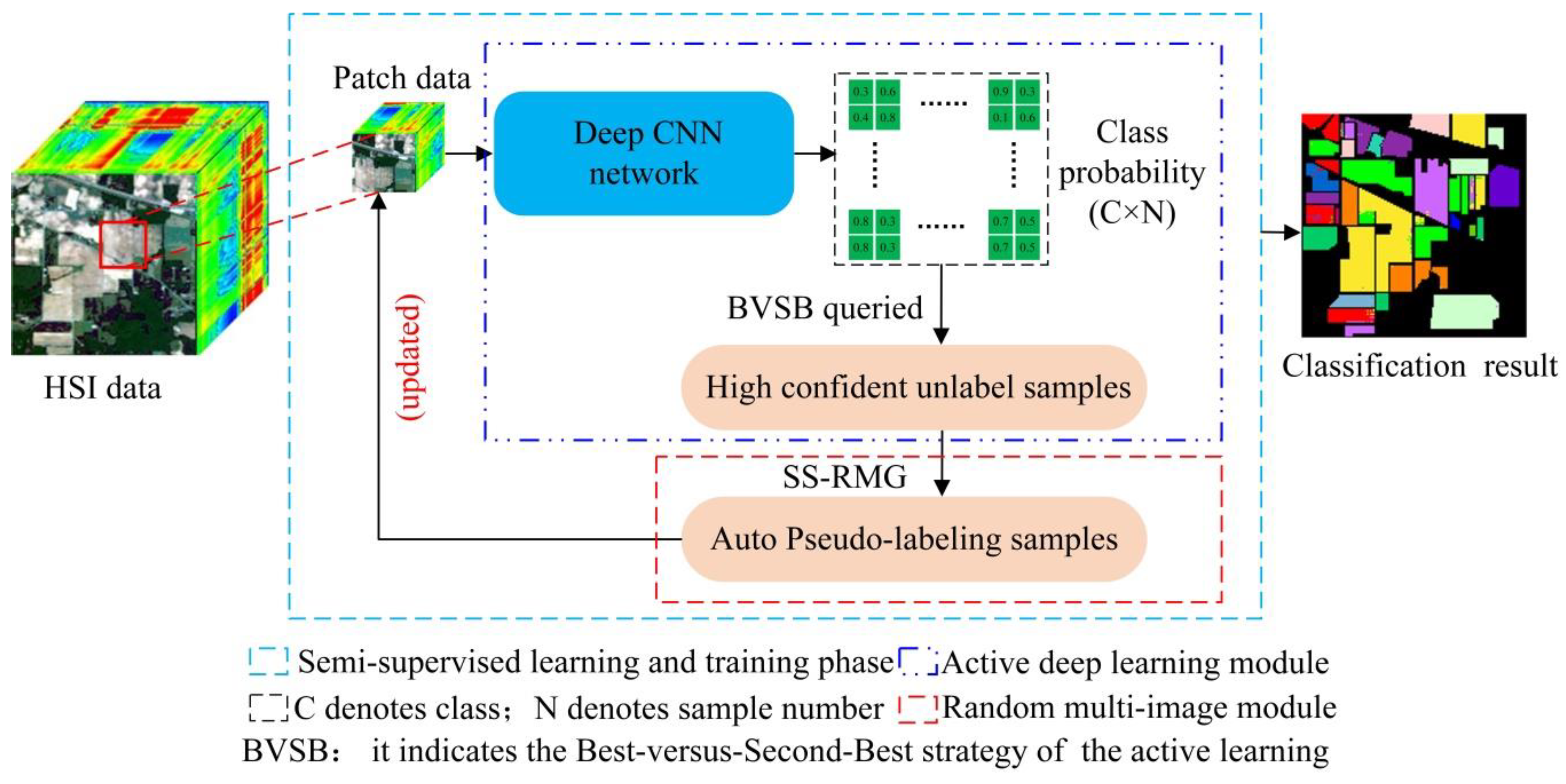
Assume that the hyperspectral dataset is , where the size of the spatial image is H × W, B is the number of spectral channels. First, HSI dataset is divided into the labeled samples set and unlabeled samples set. Next, we expanded the labeled samples set to get the extended dataset DA, which was used to initialize the CNN. Then, we input the unlabeled samples into the CNN and actively queried the most informative or the useful samples, according to the category probabilities provided by the CNN. Finally, these valuable samples were labeled through the random multi-graphs algorithm. Thereafter, we added pseudo-labeled samples to the labeled samples set, which was further used for the next iteration round of CNN training. This process was repeated until the stop condition was met. The following is a description of each part of this method.
3.2. The Introduction of Different Modules in Proposed Model
3.2.1. Active Deep Learning (ADL) Module
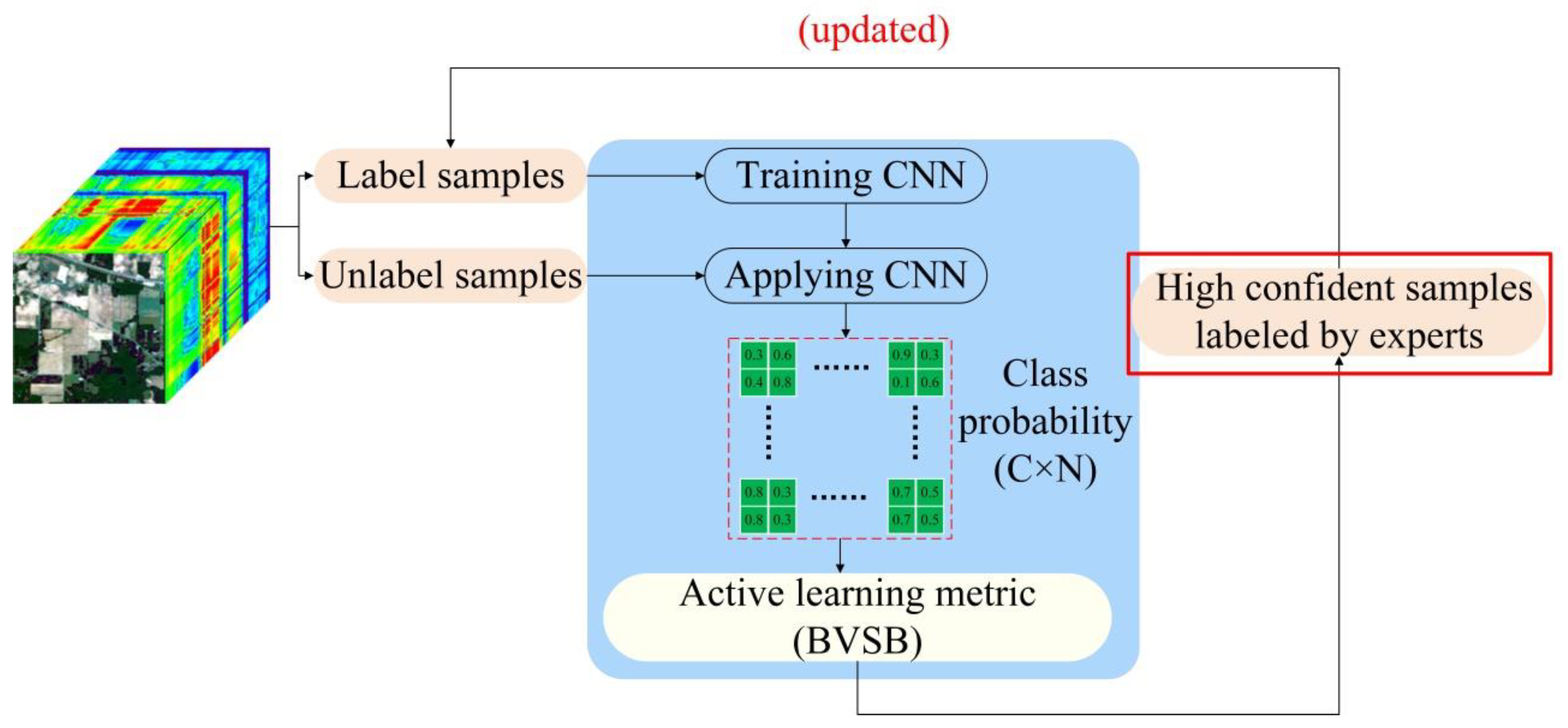
The paper proposes an improved ADL semi-supervised classification framework based on the traditional ADL classification model shown in Figure 2, where the red rectangle indicates the deficiency of traditional ADL. The following is a detailed theoretical introduction of the active deep learning module in Figure 1.
Data augmentation (DA) is widely used in the field of hyperspectral image data classification. It is often used as a means to expand the dataset and improve the accuracy. In this paper, the DA method was utilized to expand training samples by flipping horizontally or vertically in the literature [30], and the specific rotation angle can be adjusted according to the characteristics of the actual training sample. DA will also refine the classification accuracy by adding an appropriate number of samples to assist the training model during each iteration.
The objective function of the CNN classification model is defined as shown in Equation (1):
where FΘ is a nonlinear function of the CNN using parameters Θ, is the unary term that predicts the samples by using CNN, and can make adjacent samples to have the similar label. Here, the detailed explanation of label Y and the parameter Θ refers to the ADL classification method from [33]. The data input to the convolutional neural network is provided in the form of a three-dimensional cubic block with a three-dimensional convolutional kernel for convolution and pooling. Subsequently, the output of the network is selected to be a Softmax function defined as:
where is the output value of the ith node, C is the number of output nodes (e.g., the number of categories of the classification) The output value of the multiclassification is converted into a probability distribution in the range of [0, 1], with a sum of 1, by the Softmax function.
AL is a widely used strategy that selects the sample with the least confidence in an iterative manner. As we can retrieve category membership probability estimates from CNNs, this paper uses some AL metrics about the class probabilities as well (e.g., the Entropy (EP) metric and the Best-versus-Second-Best (BVSB) metric in probability-based heuristics). Both of these criteria can provide a basis for selecting the informative candidates for querying annotations. These two learning strategies are introduced in details below.
(1) EP measure: EP measures the uncertainty of class membership, and the sample has a higher EP value with the greater the uncertainty of class. Each unlabeled sample corresponds to a variable , and we obtain z distribution of P with the calculated estimated probability of class affiliation, that is , where denotes the element of the variable . The specific calculation of EP value is shown in Equation (3):
(2) BVSB measure: by calculating the difference between the most similar categories, the information content of the sample is determined. If the BVSB value of the sample is small, the sample has a large amount of information. The formula is shown in Equation (4) below:
3.2.2. Spatial and Spectral Random Multi-Graph (SS-RMG) Module
This paper uses the SS-RMG module to improve the expert marking action in traditional ADL, shown in the red box in Figure 2. The following is a detailed theoretical introduction of the Random multi-graph module in Figure 1.
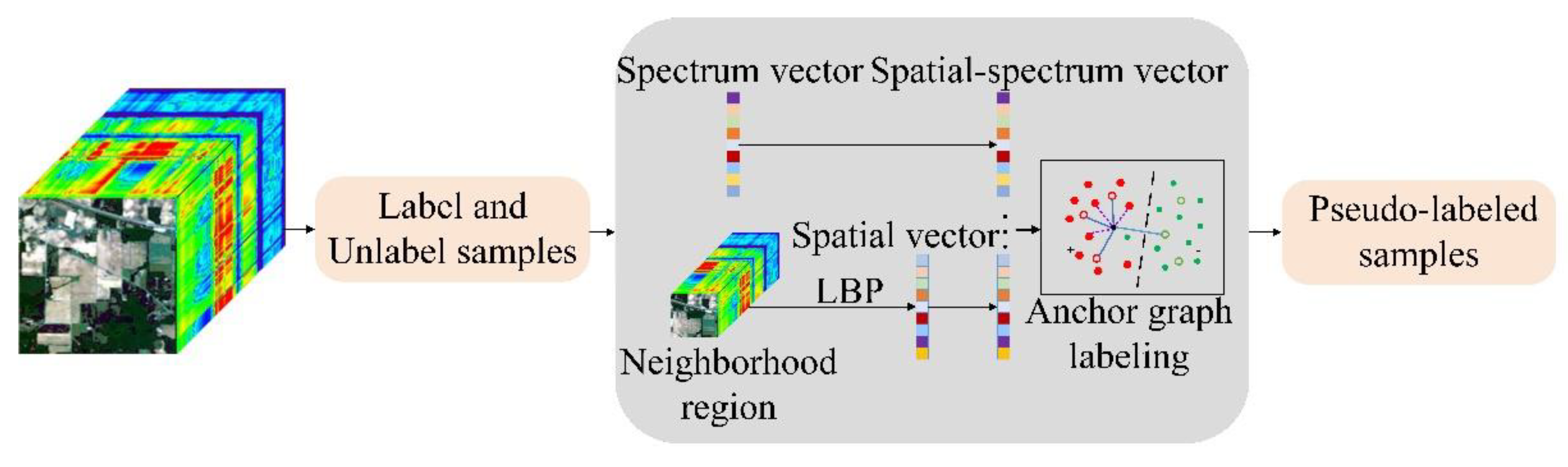
Spectral features of finite labelled samples and the spatial features of hyperspectral data, extracted by local binary patterns (LBP) [35], are extracted separately, according to the Li et al. [36] methodology. Then, the spatial and spectral joint features are utilized as the input into random multi-graphs (RMG) for classification. In this study, the graph was constructed by randomly selecting a subset of features by using the anchor graph algorithm. Then, labels of unlabeled samples were predicted based on the objective function.
(1) Data feature extraction: spectral feature extraction is all spectral bands in HSI data. After the principal component analysis, the spatial information of the spectral bands was extracted using LBP. This was an operator for describing the local texture features of an image. Here, we opted for the improvement of the original LBP, namely, equivalence pattern. The improved equivalent mode of LBP implied that, when the cyclic binary number, corresponding to certain LBP, changes from 0 to 1 or from 1 to 0, in at most two transitions, the binary corresponding to the LBP became an equivalent mode.
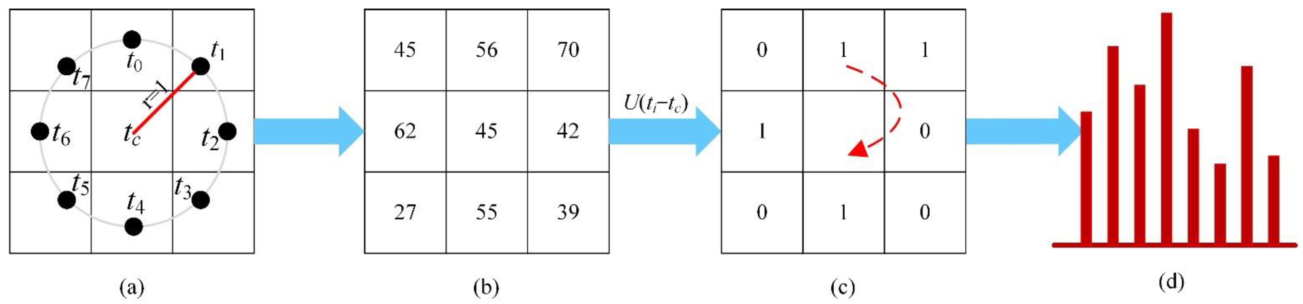
For the center pixel , the center pixel was applied as the threshold, while the position of the pixel was marked as “1” or “0”. This depends on whether the neighboring pixel value is greater than the threshold or not. By assuming that p adjacent pixels were generated by a circle with as the center and radius r, the LBP code of the central pixel can be expressed by Equation (5):
The LBP algorithm expresses the spatial information characteristics of the image with a local region of size , where the local area k is a custom parameter. Then, the histogram of each area is calculated, and the statistical histogram is connected to a feature vector, that is, the spatial feature vector. Schematic diagram of LBP is shown in Figure 3. Such improvements greatly reduce the number of binary patterns from to . Subsequently, the information is preserved, while the dimensionality of the feature vector is reduced.
(2) Random multi-graph algorithm defined the following symbols: a weighted graph can be obtained from a dataset consisting of labeled data and unlabeled data . Here, the vertices of the graph represent N data points, and the edges of the graph are formalized by a matrix of weights , which expresses the similarity between the associated nodes, and if the weight is larger, the adjacent vertices and are considered to have the same label.
The traditional graph-based semi-supervised learning approach is formulated as the following quadratic optimization problem, whereas the objective function of C-classification semi-supervised learning can be defined by Equation (6):
where is the tracking function, is the label prediction matrix, , is a diagonal matrix with the diagonal element. is the regularization matrix, representing the Laplacian graph, defined as , where W is the weight matrix of the graph.
The anchor graph algorithm was used according to the high dimensional characteristics of hyperspectral data in this study to construct and to learn the graph. The anchor graph algorithm makes the label prediction function a weighted average of the labels on a subset of anchor point samples. Thus, the label prediction function can be represented by a subset . The is an anchor point, and the label prediction function can be formalized by Equation (7):
where is the data adaptive weight, defining the vector and the vector , so that Equation (7) is rewritten to Equation (8):
Equation (8) indicates that the solution space for the unknown labels is reduced from to , and these anchor points are used as K-means clustering centers to realistically represent the data stream shape. The matrix is the data-anchor mapping matrix to be learned, and the matrix P is written in the paper, using the definition of kernel-based functions from the Nadaraya–Watson kernel regression, as shown in Equation (9):
where a Gaussian kernel function with bandwidth σ is used as the kernel regression, is the r-nearest neighbor anchor point of . It is usually considered that for , where it is considered that is larger if and are close to each other and vice versa.
A previous study [31] applied the Local Anchor Embedding algorithm to retrieve anchor points, and the data-anchor mapping problem can be formulated by Equation (10):
where is the data matrix, each row in the matrix is a data sample, is the anchor matrix, each row in the matrix represents an anchor, is the learnable data-anchor mapping matrix.
According to the matrix P, its adjacency matrix W can be designed, as indicated by Equation (11):
The diagonal matrix is defined by Equation (12):
According to the anchor’s label prediction model, the is solved first, and then, the labels of other data points can be found using Equation (8), and the objective function of is defined by Equation (13):
where is the submatrix of P, is the label of the labeled data, is the Frobenius norm of the matrix, and γ is the regularization factor. If we let , according to Equation (11), the graph Laplacian matrix is , then:
Letting the partial derivative w.r.t equal to 0, we obtain:
The label of the unlabeled sample can be predicted by the following Equation (16):
where represents the row of the P matrix and represents the column of the matrix. Figure 4 shows the SS-RMG module of classification model.
4. Experiments and Result
This paper first introduces three available HIS datasets and then discusses the setting of related parameters. Specifically, the method of selecting training samples is what percentage is taken for each category, while the specific land cover types, training, and test sets are shown in Table 1, Table 2 and Table 3. Then, we challenge the proposed model against other methods, including Edge-Preserving Filtering (EPF) [37], Image Fusion and Recursive Filtering (IFRF) [38], RP-Net [39], CNN-AL [30], and SS-RMG [23].
Numerical comparison of all methods was conducted by using the following criteria: the Overall Accuracy (OA) refers to the ratio of the total number of the correctly classified samples to that of all test samples. The Kappa coefficient is based on the confusion matrix. We calculated the Kappa coefficient to indicate whether the model predictions agreed with the actual classification results. Unlike the overall classification accuracy, which only considers the number of correctly classified pixels in the diagonal direction, the Kappa coefficient considers the missed and misclassified pixels. Class Accuracy (CA) allows for evaluating the classification accuracy of each specific class of land cover. Hereafter, larger values indicate better classification performance for all criteria in the paper.
4.1. Description of the Dataset
The first dataset is the Indian Pines dataset, and this scene was gathered by the Airborne Visible/Infrared Imaging Spectrometer (AVIRIS) sensor in Indiana (U.S.). The dataset contains 145 × 145 pixels and 220 spectral reflectance bands in the wavelength range of 0.4–2.5 μm. The remaining 200 bands are studied by excluding 20 water absorption bands. The existing features were classified into 16 classes, while the specific land cover types, training, and test sets are shown in Table 1. Also, the different colors in the second column from Table 1, Table 2 and Table 3 represent different feature categories, which are consistent with the color marks in ground-truth map.
The second dataset was obtained from the Pavia University, retrieved from the Reflection Optical System Imaging Spectrometer sensor measurements. The number of spectral bands for the Pavia University dataset was 103, and the wavelength range was 0.43–0.86 μm. The total number of pixel points for Pavia University were 610 × 610, after removing the noise-affected bands and before analysis, changing the spatial dimensions of Pavia University to 610 × 340. This scenario had nine land cover categories. The specific land covers, training, and test sets are shown in Table 2.
The third dataset is the Kennedy Space Center (KSC), which is data collected by the NASA AVIRIS (Airborne Visible/Infrared Imaging Spectrometer) instrument at the Kennedy Space Center (KSC) in Florida. AVIRIS acquired 224 bands with wavelengths between 0.40–2.50 μm. After removing the absorbance and low SNR bands, 176 bands were used for analysis. The similarity of spectral characteristics of some vegetation types made it difficult to distinguish land cover in this environment. Thirteen land cover categories were defined for the site for classification purposes. The specific land covers, training, and test sets are shown in Table 3.
4.2. Analysis of Experimental Parameters
At the ADL stage, the number of initialization samples is essential for the selection of samples in subsequent AL. The number of iterations in our study was determined as 5, with 800, 200, 200, 200, and 200 epochs set for each round given the deep learning training time. For the AL strategy, we opted the BVSB strategy that allows for efficiently determining the information content of the samples, according to the common calculation formula.
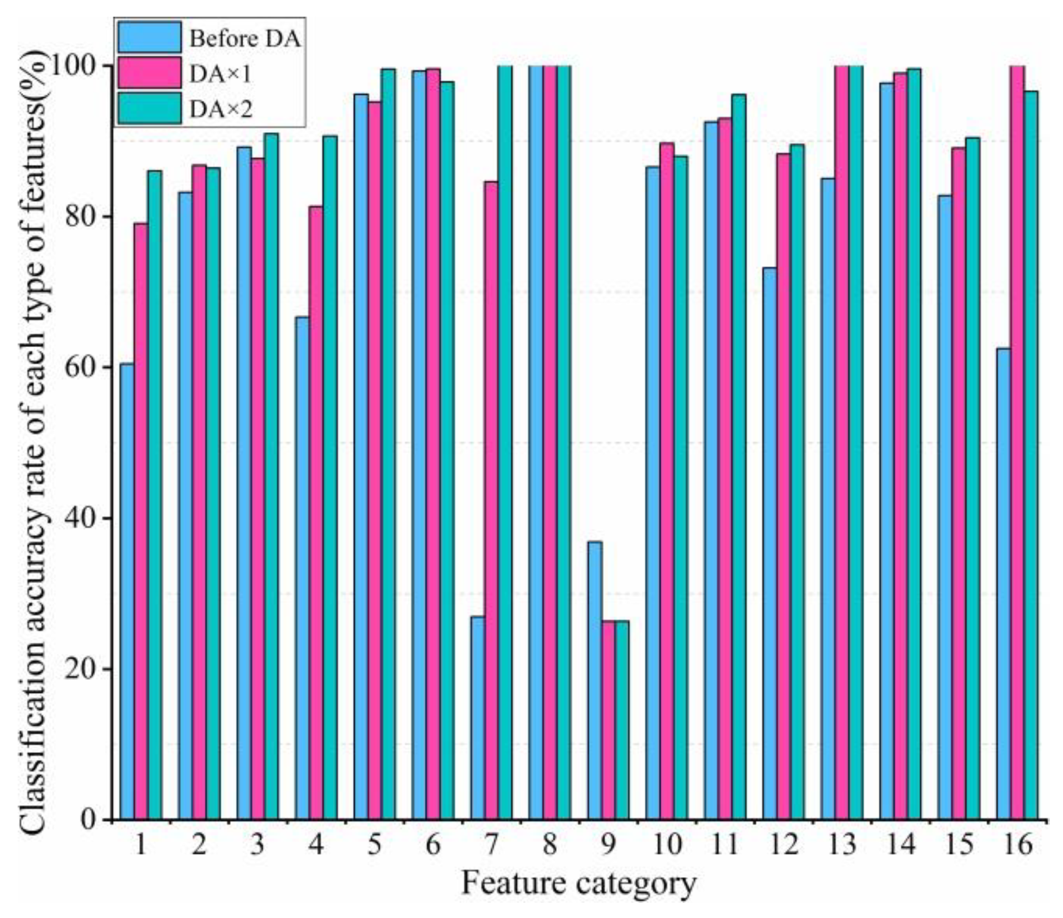
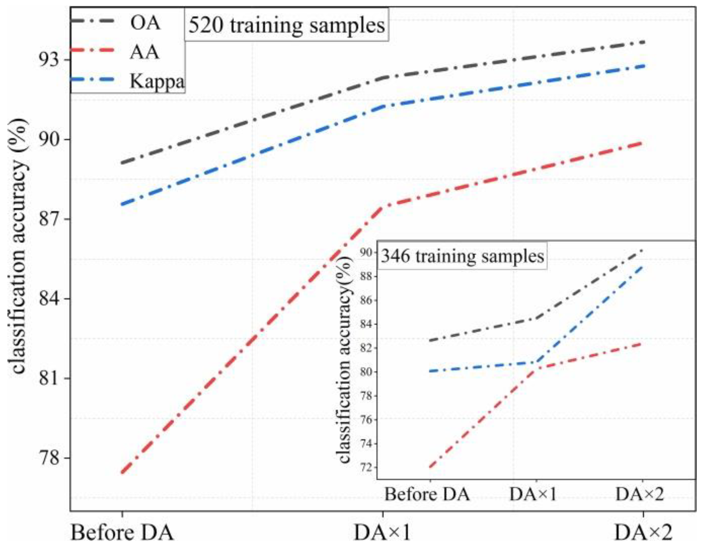
It also makes use of the DA strategy by rotating the data patch by 180° and 270°, randomly, to increase the number of training samples in this paper. In order to verify the performance of DA, the CNN model was used for the first round of training on the Indian Pines dataset. It can be seen from Figure 5 that DA strategy has a good classification result at the first round because more training samples are added to train CNN. More specifically, from Figure 6, OA can first increase 7% with 346 training samples, which shows that DA strategy can improve the classification performance greatly.
We followed the previous study experience [23], based on which, at the semi-supervised learning stage, we selected the same parameter settings, including the same number of graphs in LBP feature extraction, the number of spectral bands (Band_num), and the size of patches. The accuracy of labeling the unlabeled samples, using the random multi-graphs algorithm, had an important impact on the final classification performance. The added pseudo-labeled samples can help improve the performance of the classification model during high labeled classification accuracy. Table 4 shows how the specific experimental parameters were established. The accuracy of the pseudo-labeled samples on the three datasets were 96.36%, 93.91%, and 97.83%.
Equations (8) and (11) indicate that the design of the matrix P was related to both the construction of the adjacency matrix W and to final label prediction results. Hence, experiments compared the effect of the matrix P, defined by the Gaussian kernel, and the optimized matrix P by the local anchor embedding algorithm on the classification accuracy. Table 5 shows the overall classification accuracy results retrieved by the two methods on three different datasets. The comparison of the classification results indicates that solving the matrix P, using the Gaussian kernel definition, leads to higher classification accuracy. Moreover, the accuracy on the three datasets is correspondingly improved. Due to this, we opt for the Gaussian kernel definition to solve the matrix P in all the subsequent experiments.
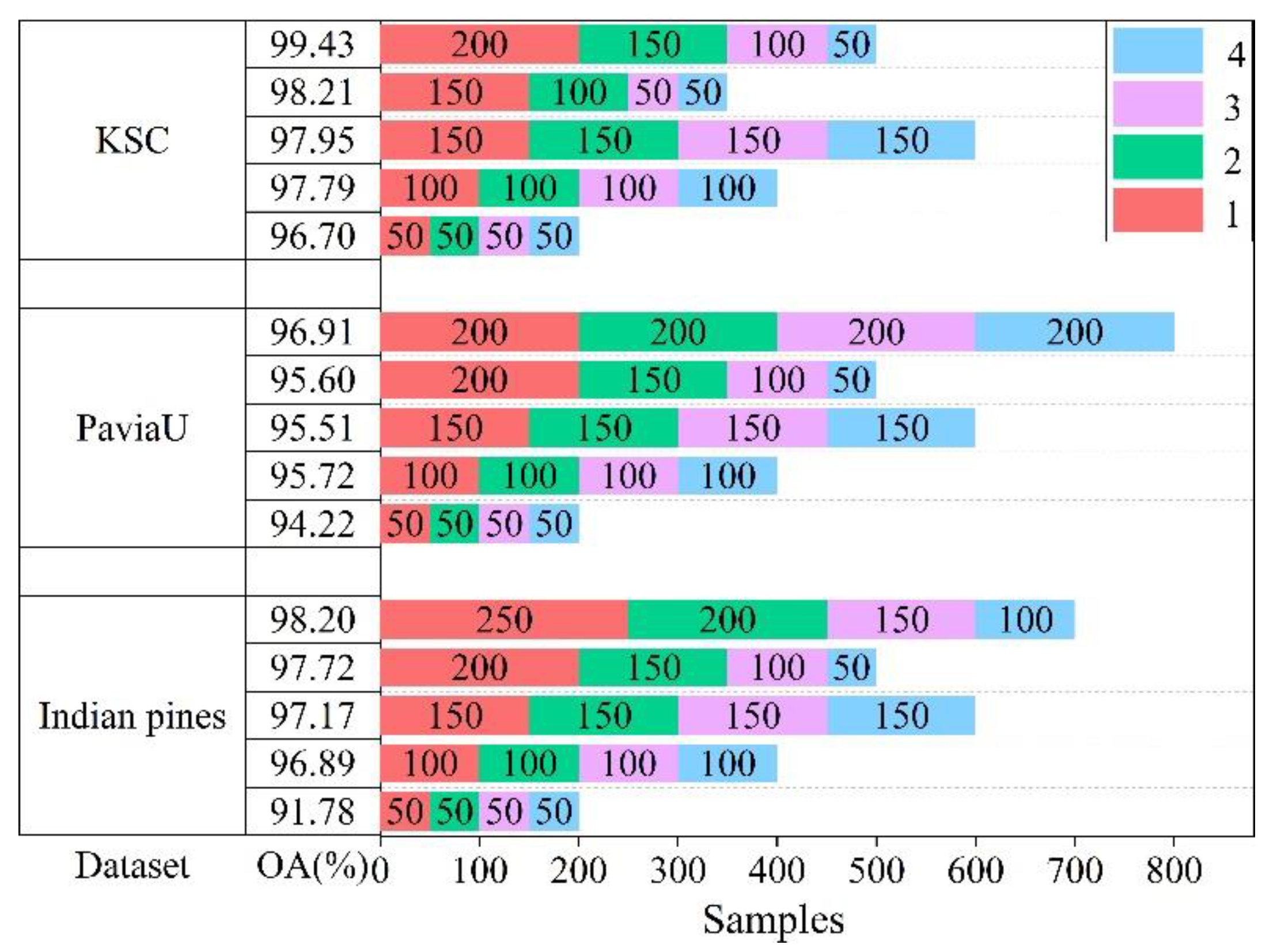
In the experiment, we need to select a certain number of pseudo-labeled samples to expand the training set. However, very unlike the types and distributions of features in a different dataset, the experiment demands one to determine the number of pseudo-label samples that will be added to the training set in a different dataset separately, which can obtain a model with better generalization performance. What’s more, we decided to set the number of pseudo-labeled samples to a multiple of 50 on the three datasets, according to the minimum batch of 50 in CNN training. Through multiple experiments, we selected five of the experimental results, as shown in Figure 7.
The Indian pines dataset analysis indicates that the classification accuracy tended to increase with the increase in unlabeled samples. Overall, a good classification result of 98.20% was achieved when 250, 200, 150, and 100 samples were added to the training set. However, for the Pavia University dataset, with the increase in unlabeled samples, the third experiment and the fourth experiment did not provide higher classification results. By adjusting the number of samples added at each time to 200, the experiments provided higher classification accuracy, which alleviated the mislabeling problem. This problem was driven by the semi-supervised algorithm when labeling unlabeled samples. For the KSC dataset, the number of samples added in each round was determined to be 200, 150, 100, and 50, while the classification accuracy reached 99.43%.
4.3. Classification Results
We applied the new ADL method on three datasets and further compared it with related hyperspectral image data classification methods, including the EPF [37], IFRF [38], RP-Net [39], CNN-AL [30], and SS-RMG [23]. EPF optimizes the classification results by pixel in the local filtering framework, and the pixel-level spectral information is more advantageous relative to the spatial information in the spectral-spatial classification. IFRF performs classification by combining spatial and spectral features through image fusion and recursive filtering. RP-Net performs classification by combining shallow and deep convolutional features, using random patches taken directly from images as convolutional kernels. CNN-AL is a combination of active learning and a convolutional neural network to achieve good classification results for small sample cases. SS-RMG stacks spectral features and spatial features, and it applies the random multi-graphs algorithm for classification.
We selected training and test samples proportionally, ran each of the mentioned methods for five times and reported their average test classification correctness. We also selected overall accuracy (OA), individual category accuracy (CA), and Kappa coefficient (Kappa) as the criteria for quantitative evaluation.
4.3.1. Experimental Analysis of the Indian Pines Dataset
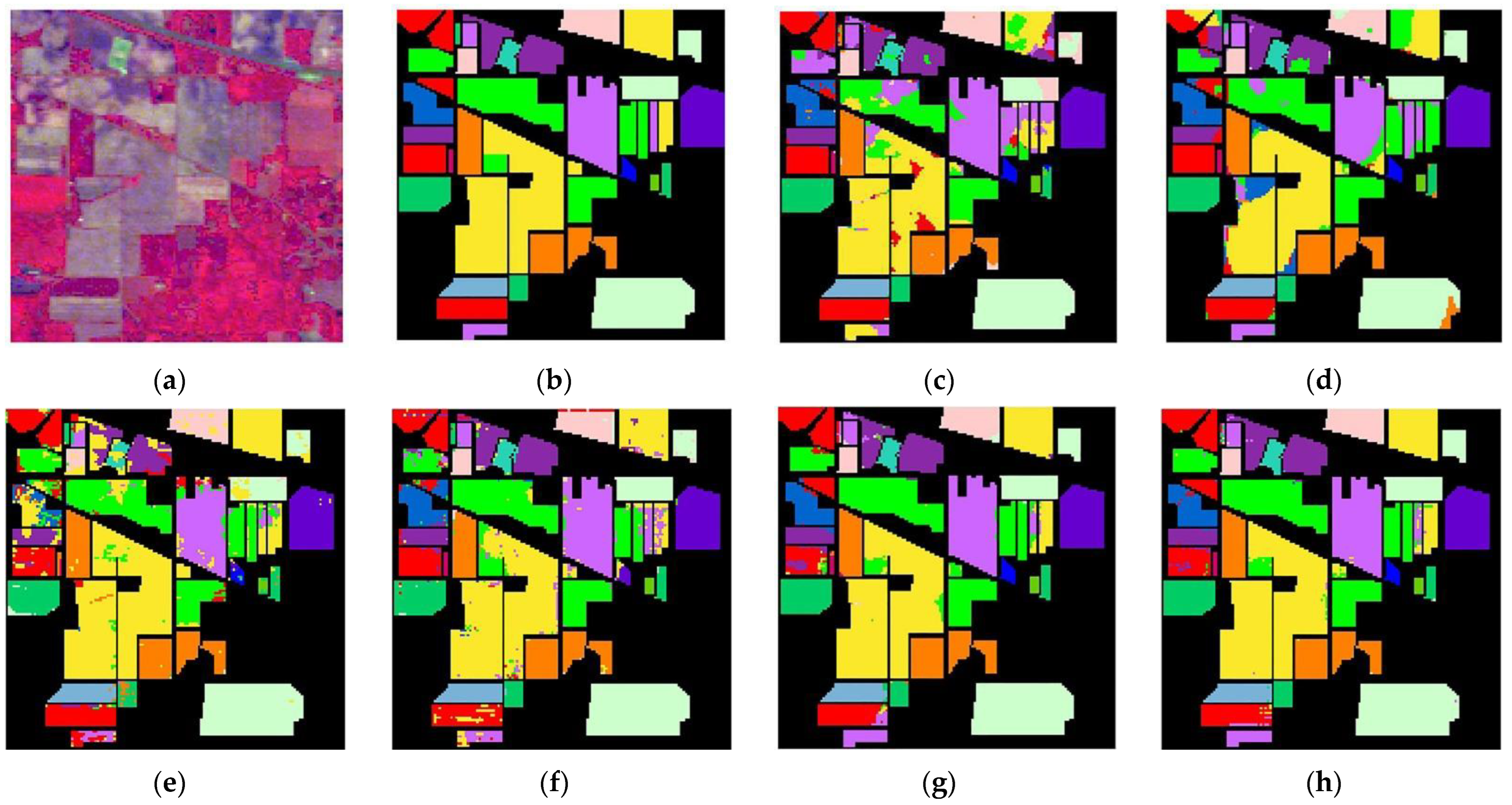
In the training sample set, 3.3% of the labeled samples were used, and the rest of samples were test samples in the Indian Pines dataset. Table 1 lists the number of training samples and test samples of each type of ground feature in the Indian dataset. Therefore, in the first round, 346 labeled training samples were added to initialize the CNN model. Pseudo-label samples, added in each round of the training process of the proposed method, were 250, 200, 150, 100. Table 6 shows the comparison of the classification accuracy of each classification method with the same number of labeled samples. The classification plots of all methods are illustrated in Figure 8.
The analysis of the experimental results (Table 6) includes the name of each category of features, the classification accuracy of each feature, corresponding to the different classification methods, and the total accuracy OA and Kappa coefficient under the different classification methods. There are 16 classes of features in the Indian dataset. Table 6 results prove that the final classification accuracy OA improved to 98.20%, and the Kappa coefficient improved to 97.94 with the proposed method. Compared with the SS-RMG classification method, our new method improved, at least, by 1.8% in OA. Table 1 also shows that the samples of some ground objects are very rare. For instance, the first type Alfalfa had only 46 samples, the seventh type Grass-pasture-mowed had only 28 samples, and the ninth type Oats had only 20 samples. As the number of samples of each type of feature may vary, the classification accuracy cannot be improved due to the limitation of the number of samples. However, the method proposed in this paper was used to classify the first, seventh, and ninth types of features. Compared with other classification methods, the classification accuracy of the three types of features has been greatly improved, and the new classification accuracy has reached 100%. As seen, the proposed classification method yields superior results.
4.3.2. Experimental Analysis of the Pavia University Dataset
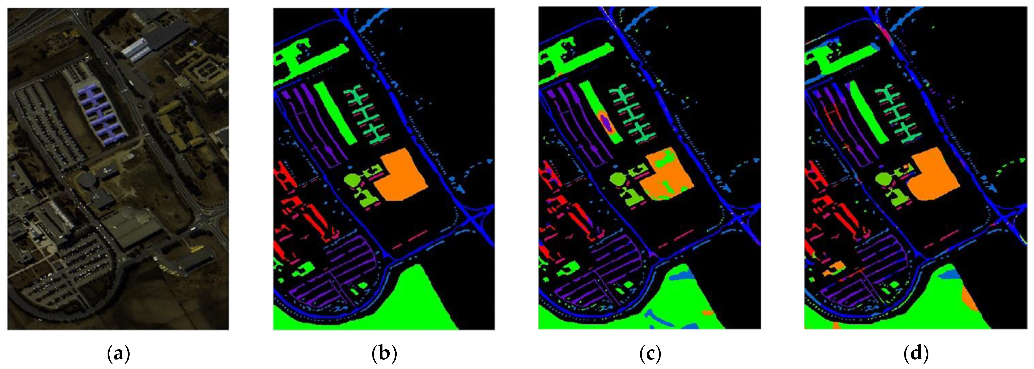
In the training sample set, 0.5% of the labeled samples were used, and the rest of samples were test samples in the Pavia University dataset. Table 2 displays the number of training samples and test samples of each type of feature in the Pavia University dataset. Therefore, in the first round, 219 labeled training samples were added to initialize the CNN model. The Pseudo-label samples were 200, 200, 200, and 200.
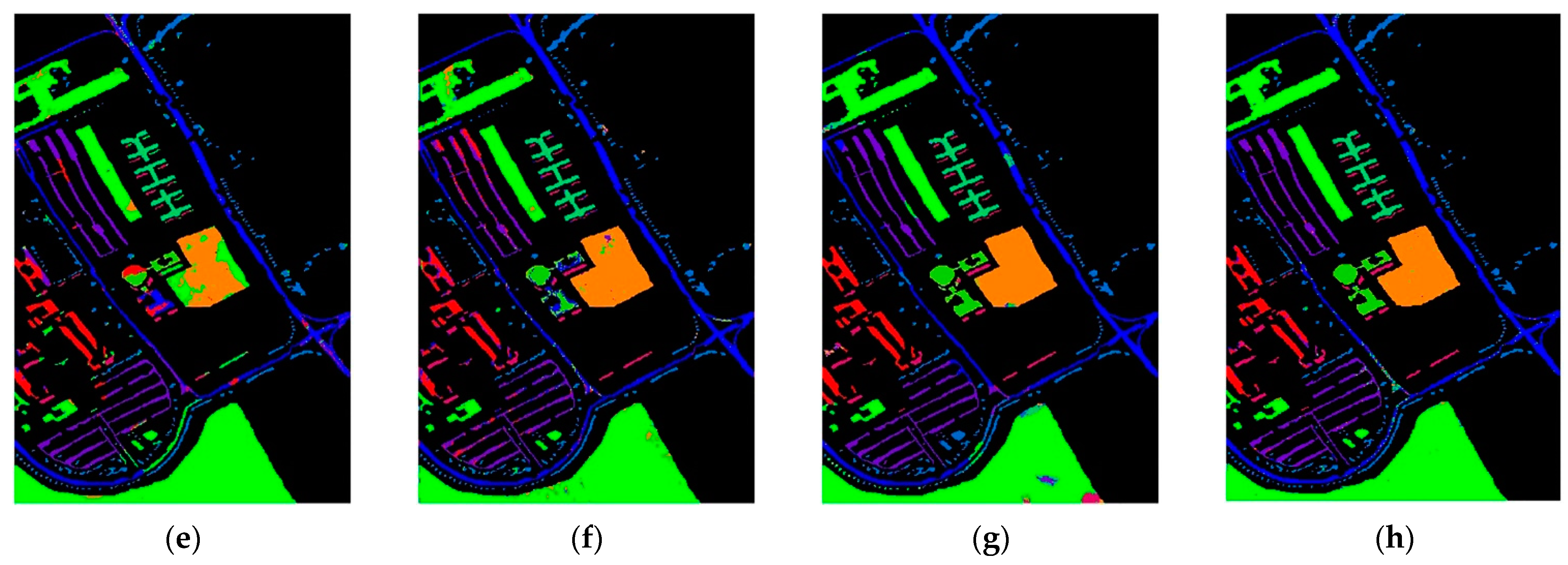
Table 7 demonstrates the comparison of the classification accuracy of each classification method for the same number of labeled samples, while the classification plots of all methods are shown in Figure 9. Table 7 (the analysis of the experimental results) includes the name of each category of features, the classification accuracy of each feature corresponding to the different classification methods, and the total accuracy OA and Kappa coefficient under the different classification methods. There were nine classes of features in the Pavia University dataset. As shown in Table 7, the classification accuracy of each class of features has been improved (at different rates) under the proposed classification model. Compared with EPF and IFRF, using support vector machine classification, the new ADL classification model stood out with more advantages. Moreover, it had better generalization performance in the case of small samples. Thus, the full use of a large number of unlabeled samples could be achieved, while the problem of scarcity of labeled samples in HSI classification could be simultaneously solved.
4.3.3. Experimental Analysis of the Kennedy Space Center Dataset
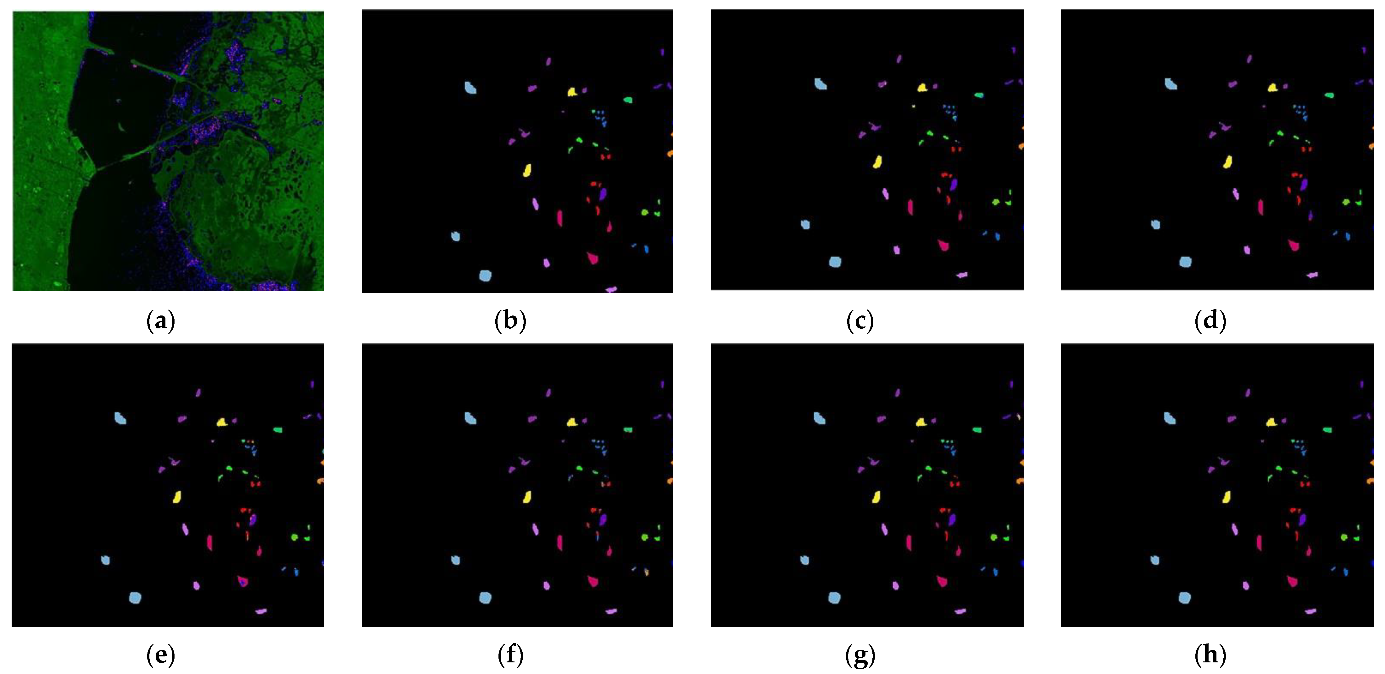
In the training set, 0.5% of the labeled samples were used, and the rest of samples were test samples in the Kennedy Space Center dataset. Table 3 shows the number of training samples and test samples of each type of feature in the Kennedy Space Center dataset. Therefore, in the first round, 180 labeled training samples were added to initialize the CNN model. The Pseudo-label samples were 200, 150, 100, and 50. Table 8 shows the comparison of the classification accuracy of each classification method with the same number of labeled samples, while the classification plots of all methods are illustrated in Figure 10.
Table 8 (the analysis of the experimental results) includes the name of each class of features, the classification accuracy of each feature, corresponding to the different classification methods, and the total accuracy OA and Kappa coefficient under the different classification methods. Both the KSC dataset and the Indian Pines dataset were photographed and collected by the AVIRIS sensors. However, as seen from Table 3, the number of the samples of each type of feature in this dataset is more balanced. Overall, the new method exhibits superior performance on the KSC dataset, with a classification accuracy OA of 99.43% and a Kappa coefficient of 99.36. To sum up, the classification accuracy of 9 types of features in 13 types of features reached 100%. Compared with traditional deep learning classification methods, such as RP-Net and CNN-AL, the method proposed in this paper had more advantages and can be classified with unlabeled sample features with high confidence. Experimental results showed that the new classification model proposed in this study, can classify different datasets, and the classification effect is better.
4.3.4. Analysis and Discussion
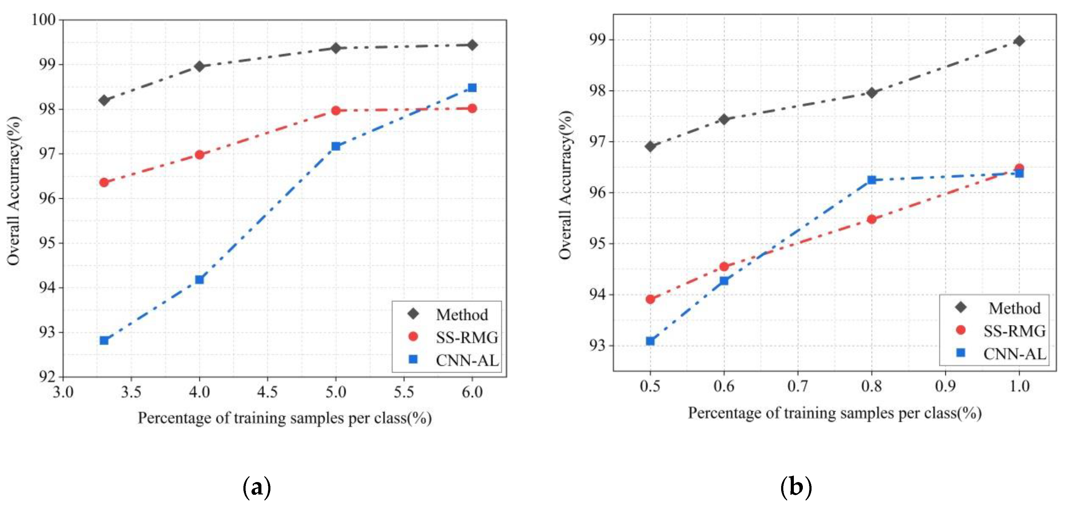
To evaluate the generalization ability and robustness of the new improved ADL classification model, we randomly selected 3.3%, 4%, 5%, and 6% labeled samples from the Indian Pines dataset. We also randomly selected the 0.5%, 0.6%, 0.8%, and 1% labeled samples from the University of Pavia dataset to be the training data. As shown in Figure 11, the paper compares the improved method with two other classification methods, of which CNN-AL is a traditional active deep learning method, and SS-RMG is a classification method that uses anchor image learning alone. The proposed model improves and combines the advantages of CNN-AL and SS-RMG.
Figure 11 shows that when the training data is small, the new method can still provide much higher classification accuracy compared with SS-RMG and CNN-AL. Overall, the experimental results confirmed that the proposed classification model achieved good classification performance not only in most categories but also in the category of features with only a small number of labeled samples. The performance improvement was driven by the following factors. First, the strategy with selection of samples in AL was introduced. Meanwhile, querying samples with greater enhancement to the classification model among unlabeled samples enabled the deep convolutional neural network to extract more discriminative features. Second, the new ADL model provided a semi-supervised learning algorithm based on anchor graphs. The graph learning was also used to pseudo-label unlabeled samples, thereby ameliorating the high labeling accuracy of the samples added to the training.
The method used in the paper is a small sample supervised classification method based on improved active deep learning. The proportion of selected training samples to the total number of samples is very small. In the semi-supervised learning process, samples are automatically selected from the test samples, labeled, and added to the training set. Although the process of selecting training samples has tried its best to reduce pixel overlap (leakage) between the training and test sets, this is due to the possible leakage of information when the neighborhood of the training and testing pixels overlap [40]. This problem will be further studied and resolved in follow-up research.
5. Conclusions
In this paper, an improved active deep learning scheme, based on the random multi-graph algorithm, is proposed to solve the unlabeled samples labeling problem in the HSI classification. Considering the disadvantages of expert labeling cost in active learning, the proposed model utilizes the concept of pseudo label to produce more training samples available automatically, thereby reducing the labeling cost of human beings and enabling machine self-learning. It is worth noting that our proposed classification model presents another thought way of active deep learning and the potential of active deep learning as a mature learning framework. Experiments, performed on three real HSIs from different scenes, confirm that the proposed method produces competitive classification performance over other compared approaches, which also illustrates the generalization capability and effectiveness of the proposed method for identifying different features. In the future research lines of this work, it is of great significance to further explore the deep learning networks, except CNN, and algorithms of machine learning pseudo labeled samples.
Author Contributions
Conceptualization, Q.W. and M.C.; methodology, Q.W. and M.C.; software and experiments, Q.W. and M.C.; validation, Q.W. and M.C.; writing—original draft preparation, Q.W. and M.C.; writing—review and editing, Q.W., M.C., J.Z. and Y.W.; funding acquisition, Q.W., J.Z., S.K. and Y.W. All authors contributed to the results analysis and reviewed the manuscript. All authors have read and agreed to the published version of the manuscript.
Funding
This work was supported in part by the Natural Science Foundation of China under Grant 61871150, in part by the Natural Foundation of Heilongjiang Province under Grant LH2019E058, in part by the Scientific Research Foundation of Harbin University of Science and Technology under Grant 217045332.
Institutional Review Board Statement
Not applicable.
Informed Consent Statement
Not applicable.
Data Availability Statement
Not applicable.
Conflicts of Interest
The authors declare no conflict of interest.
References
- Yuan, Q.; Shen, H.; Li, T. Deep learning in environmental remote sensing: Achievements and challenges. Remote Sens. Environ. 2020, 241, 111716. [Google Scholar] [CrossRef]
- He, L.; Li, J.; Liu, C.; Li, S. Recent Advances on Spectral-Spatial Hyperspectral Image Classification: An Overview and New Guidelines. IEEE Trans. Geosci. Remote Sens. 2018, 56, 1579–1597. [Google Scholar] [CrossRef]
- Hong, D.; Yokoya, N.; Ge, N.; Chanussot, J.; Zhu, X.X. Learnable manifold alignment (LeMA): A semi-supervised cross-modality learning framework for land cover and land use classification. ISPRS J. Photogramm. Remote Sens. 2019, 147, 193–205. [Google Scholar] [CrossRef]
- Alcolea, A.; Paoletti, M.E.; Haut, J.M.; Resano, J.; Plaza, A. Inference in supervised spectral classifiers for on-board hyperspectral imaging: An overview. Remote Sens. 2020, 12, 534. [Google Scholar] [CrossRef] [Green Version]
- Matsuki, T.; Yokoya, N.; Iwasaki, A. Hyperspectral tree species classification of Japanese complex mixed forest with the aid of LiDAR data. IEEE J. Sel. Top. Appl. Earth Observ. Remote Sens. 2015, 8, 2177–2187. [Google Scholar] [CrossRef]
- Hong, D.; Yokoya, N.; Chanussot, J.; Zhu, X. CoSpace: Common subspace learning from hyperspectral multispectral correspondences. IEEE Trans. Geosci. Remote Sens. 2019, 57, 4349–4359. [Google Scholar] [CrossRef] [Green Version]
- Chen, M.; Wang, Q.; Li, X. Discriminant analysis with graph learning for hyperspectral image classification. Remote Sens. 2018, 10, 836. [Google Scholar] [CrossRef] [Green Version]
- Licciardi, G.; Marpu, P.R.; Chanussot, J.; Benediktsson, J.A. Linear versus nonlinear PCA for the classification of hyperspectral data based on the extended morphological profiles. IEEE Geosci. Remote Sens. Lett. 2012, 9, 447–451. [Google Scholar] [CrossRef] [Green Version]
- Bandos, T.; Bruzzone, L.; Camps-Valls, G. Classification of hyperspectral images with regularized linear discriminant analysis. IEEE Trans. Geosci. Remote Sens. 2009, 47, 862–873. [Google Scholar] [CrossRef]
- Bazine, R.; Wu, Q.; Boukhechba, K. Spectral DWT multilevel decomposition with spatial filtering enhancement preprocessing-based approaches for hyperspectral imagery classification. Remote Sens. 2019, 11, 2906. [Google Scholar] [CrossRef] [Green Version]
- Qi, W.; Zhang, X.; Wang, N.; Zhang, M.; Cen, J. A Spectral-Spatial Cascaded 3D Convolutional Neural Network with a Convolutional Long Short-Term Memory Network for Hyperspectral Image Classification. Remote Sens. 2019, 11, 2363. [Google Scholar] [CrossRef] [Green Version]
- Hu, Y.; An, R.; Wang, B.; Xing, F.; Ju, F. Shape Adaptive Neighborhood Information-Based Semi-Supervised Learning for Hyperspectral Image Classification. Remote Sens. 2020, 12, 2976. [Google Scholar] [CrossRef]
- Wei, L.; Du, Q. Gabor-filtering-based nearest regularized subspace for hyperspectral image classification. IEEE J. Sel. Top. Appl. Earth Obs. Remote Sens. 2014, 7, 1012–1022. [Google Scholar]
- Chen, Y.; Lin, Z.; Zhao, X.; Wang, G.; Gu, Y. Deep learning-based classification of hyperspectral data. IEEE J. Sel. Top. Appl. Earth Observ. Remote Sens. 2014, 7, 2094–2107. [Google Scholar] [CrossRef]
- Chen, Y.; Zhao, X.; Jia, X. Spectral–spatial classification of hyperspectral data based on deep belief network. IEEE J. Sel. Top. Appl. Earth Observ. Remote Sens. 2015, 8, 2381–2392. [Google Scholar] [CrossRef]
- Wang, Q.; Yuan, Z.; Du, Q.; Li, X. GETNET: A general end-to-end 2-D CNN framework for hyperspectral image change detection. IEEE Trans. Geosci. Remote Sens. 2019, 57, 3–13. [Google Scholar] [CrossRef] [Green Version]
- Hamida, A.B.; Benoit, A.; Lambert, P.; Amar, C.B. 3-D deep learning approach for remote sensing image classification. IEEE Trans. Geosci. Remote Sens. 2018, 56, 4420–4434. [Google Scholar] [CrossRef] [Green Version]
- Cui, X.; Zheng, K.; Gao, L.; Zhang, B.; Yang, D.; Ren, J. Multiscale spatial-spectral convolutional network with image-based framework for hyperspectral imagery classification. Remote Sens. 2019, 11, 2220. [Google Scholar] [CrossRef] [Green Version]
- Liu, K.; Xu, Q.; Wang, Z. Survey on active learning algorithms. Comput. Eng. Appl. 2012, 48, 1–4. [Google Scholar]
- Wang, G.; Ren, P. Hyperspectral Image Classification with Feature-Oriented Adversarial Active Learning. Remote Sens. 2020, 12, 3879. [Google Scholar] [CrossRef]
- Liu, C.; Li, J.; He, L. Superpixel-Based Semisupervised Active Learning for Hyperspectral Image Classification. IEEE J. Sel. Top. Appl. Earth Obs. Remote Sens. 2019, 12, 357–370. [Google Scholar] [CrossRef]
- Liu, X.; Zhang, J.; Li, T.; Zhang, Y. A Novel Synergetic Classification Approach for Hyperspectral and Panchromatic Images Based on Self-Learning. IEEE Trans. Geosci. Remote Sens. 2016, 54, 4917–4928. [Google Scholar] [CrossRef]
- Gao, F.; Wang, Q.; Dong, J.; Xu, Q. Spectral and Spatial Classification of Hyperspectral Images Based on Random Multi-Graphs. Remote Sens. 2018, 10, 1271. [Google Scholar] [CrossRef] [Green Version]
- Yue, J.; Zhao, W.; Mao, S.; Liu, H. Spectral–spatial classification of hyperspectral images using deep convolutional neural networks. Remote Sens. Lett. 2015, 6, 468–477. [Google Scholar] [CrossRef]
- Cao, X.; Zhou, F.; Xu, L.; Meng, D.; Xu, Z.; Paisley, J. Hyperspectral image classification with Markov random fields and a convolutional neural network. IEEE Trans. Image Process 2018, 27, 2354–2367. [Google Scholar] [CrossRef] [PubMed] [Green Version]
- Stumpf, A.; Lachiche, N.; Malet, J.; Kerle, N.; Puissant, A. Active learning in the spatial domain for remote sensing image classification. IEEE Trans. Geosci. Remote Sens. 2014, 52, 2492–2507. [Google Scholar] [CrossRef]
- Pasolli, E.; Melgani, F.; Tuia, D.; Pacifici, F.; Emery, W.J. SVM active learning approach for image classification using spatial information. IEEE Trans. Geosci. Remote Sens. 2014, 52, 2217–2233. [Google Scholar] [CrossRef]
- Liu, P.; Zhang, H.; Eom, K.B. Active deep learning for classification of hyperspectral images. IEEE J. Sel. Top. Appl. Earth Observ. Remote Sens. 2017, 10, 712–724. [Google Scholar] [CrossRef] [Green Version]
- Haut, J.M.; Paoletti, M.E.; Plaza, J.; Li, J.; Plaza, A. Active learning with convolutional neural networks for hyperspectral image classification using a new Bayesian approach. IEEE Trans. Geosci. Remote Sens. 2018, 56, 6440–6461. [Google Scholar] [CrossRef]
- Cao, X.; Yao, J.; Xu, Z.; Meng, D. Hyperspectral Image Classification with Convolutional Neural Network and Active Learning. IEEE Trans. Geosci. Remote Sens. 2020, 58, 4604–4616. [Google Scholar] [CrossRef]
- Shi, G.; Huang, H.; Liu, J.; Li, Z.; Wang, L. Spatial-Spectral Multiple Manifold Discriminant Analysis for Dimensionality Reduction of Hyperspectral Imagery. Remote. Sens. 2019, 11, 2414. [Google Scholar] [CrossRef] [Green Version]
- Zhang, Q.; Sun, J.; Zhong, G.; Dong, J. Random multi-graphs: A semi-supervised learning framework for classification of high dimensional data. Image Vis. Comput. 2017, 60, 30–37. [Google Scholar] [CrossRef]
- Zhang, Y.; Cao, G.; Li, X.; Wang, B.; Fu, P. Active semi-supervised random forest for hyperspectral image classification. Remote Sens. 2019, 11, 2974. [Google Scholar] [CrossRef] [Green Version]
- Wang, M.; Fu, W.; Hao, S.; Tao, D.; Wu, X. Scalable semi-supervised learning by efficient anchor graph regularization. IEEE Trans. Knowl. Data Eng. 2016, 28, 1864–1877. [Google Scholar] [CrossRef]
- Ojala, T.; Peitikainen, M.; Maenpaa, T. Multiresolution gray-scale and rotation invariant texture classification with local binary pattern. IEEE Trans. Pattern Anal. Mach. Intell. 2002, 24, 971–987. [Google Scholar] [CrossRef]
- Li, W.; Chen, C.; Su, H.; Du, Q. Local binary patterns and extreme learning machine for hyperspectral imagery classification. IEEE Trans. Geosci. Remote Sens. 2015, 53, 3681–3693. [Google Scholar] [CrossRef]
- Kang, X.; Li, S.; Benediktsson, J.A. Spectral-spatial hyperspectral image classification with edge-preserving filtering. IEEE Trans. Geosci. Remote Sens. 2014, 52, 2666–2677. [Google Scholar] [CrossRef]
- Kang, X.; Li, S.; Benediktsson, J. Feature extraction of hyperspectral images with image fusion and recursive filtering. IEEE Trans. Geosci. Remote Sens. 2014, 52, 3742–3752. [Google Scholar] [CrossRef]
- Xu, Y.; Du, B.; Zhang, F.; Zhang, L. Hyperspectral image classification via a random patches network. ISPRS J. Photogramm. Remote Sens. 2018, 142, 344–357. [Google Scholar] [CrossRef]
- Nalepa, J.; Myller, M.; Kawulok, M. Validating hyperspectral image segmentation. IEEE Geosci. Remote Sens. Lett. 2019, 16, 1264–1268. [Google Scholar] [CrossRef] [Green Version]
Figure 1.
Proposed improved active deep learning semi-supervised classification framework.

Figure 2.
Active deep learning module of the classification model.

Figure 3.
Example of LBP binary thresholding: (a) central pixel tc and its eight circular neighborhoods, (b) local region block, (c) Binary label of local region, and (d) LBP histogram.
Figure 3.
Example of LBP binary thresholding: (a) central pixel tc and its eight circular neighborhoods, (b) local region block, (c) Binary label of local region, and (d) LBP histogram.

Figure 4.
SS−RMG module of classification model.

Figure 5.
Classification accuracy of each type of feature, before and after DA operation, with 520 samples.
Figure 5.
Classification accuracy of each type of feature, before and after DA operation, with 520 samples.

Figure 6.
Classification, before and after DA operation, under 346 and 520 training samples.

Figure 7.
Five experiments were performed on three datasets to determine the number of samples selected for each round of active learning strategies.
Figure 7.
Five experiments were performed on three datasets to determine the number of samples selected for each round of active learning strategies.

Figure 8.
Indian Pines dataset Classification: (a) False color image, (b) Ground-truth map, (c) EPF, (d) IFRF, (e) RPNET, (f) CNN-AL, (g) SS-RMG, and (h) Improved-ADL.
Figure 8.
Indian Pines dataset Classification: (a) False color image, (b) Ground-truth map, (c) EPF, (d) IFRF, (e) RPNET, (f) CNN-AL, (g) SS-RMG, and (h) Improved-ADL.

Figure 9.
C Pavia University dataset Classification: (a) False color image, (b) Ground-truth map, (c) EPF, (d) IFRF, (e) RPNET, (f) CNN-AL, (g) SS-RMG, (h) Improved-ADL.
Figure 9.
C Pavia University dataset Classification: (a) False color image, (b) Ground-truth map, (c) EPF, (d) IFRF, (e) RPNET, (f) CNN-AL, (g) SS-RMG, (h) Improved-ADL.


Figure 10.
Kennedy Space Center dataset Classification: (a) False color image, (b) Ground-truth map, (c) EPF, (d) IFRF, (e) RPNET, (f) CNN-AL, (g) SS-RMG, (h) Improved-ADL.
Figure 10.
Kennedy Space Center dataset Classification: (a) False color image, (b) Ground-truth map, (c) EPF, (d) IFRF, (e) RPNET, (f) CNN-AL, (g) SS-RMG, (h) Improved-ADL.

Figure 11.
Curves of overall accuracies versus different percentages of training samples, obtained by different methods on two datasets: (a) Indian Pines dataset, (b) Pavia University dataset.
Figure 11.
Curves of overall accuracies versus different percentages of training samples, obtained by different methods on two datasets: (a) Indian Pines dataset, (b) Pavia University dataset.


Table 1.
Train-test distribution of samples for the Indian Pines dataset.
| Class | Name | Train | Test | Total |
|---|---|---|---|---|
| 1 | Alfalfa | 2 | 44 | 46 |
| 2 | Corn-notill | 48 | 1380 | 1428 |
| 3 | Corn-mintill | 28 | 802 | 830 |
| 4 | Corn | 8 | 229 | 237 |
| 5 | Grass-pasture | 16 | 467 | 483 |
| 6 | Grass-trees | 25 | 705 | 730 |
| 7 | Grass-pasture-mowed | 1 | 27 | 28 |
| 8 | Hay-windrowed | 16 | 462 | 478 |
| 9 | Oats | 1 | 19 | 20 |
| 10 | Soybean-notill | 33 | 939 | 972 |
| 11 | Soybean-mintill | 82 | 2373 | 2455 |
| 12 | Soybean-clean | 20 | 573 | 593 |
| 13 | Wheat | 7 | 198 | 205 |
| 14 | Woods | 42 | 1223 | 1265 |
| 15 | Building-Grass-Trees-Drives | 13 | 373 | 386 |
| 16 | Stone-Steel-Towers | 4 | 89 | 93 |
| Total | 346 | 9903 | 10,249 |
Table 2.
Train-test distribution of samples for the Pavia University dataset.
| Class | Name | Train | Test | Total |
|---|---|---|---|---|
| 1 | Shadows | 34 | 6597 | 6631 |
| 2 | Bricks | 94 | 18,555 | 18,649 |
| 3 | Bitumen | 11 | 2088 | 2099 |
| 4 | Bare Soil | 16 | 3048 | 3064 |
| 5 | Metal sheets | 7 | 1338 | 1345 |
| 6 | Trees | 26 | 5003 | 5029 |
| 7 | Gravel | 7 | 1323 | 1330 |
| 8 | Meadows | 19 | 3663 | 3682 |
| 9 | Asphalt | 5 | 942 | 947 |
| Total | 219 | 42,557 | 42,776 |
Table 3.
Train-test distribution of samples for the Kennedy Space Center dataset.
| Class | Name | Train | Test | Total |
|---|---|---|---|---|
| 1 | Scrub | 26 | 735 | 761 |
| 2 | Willow | 9 | 234 | 243 |
| 3 | CP hammock | 9 | 247 | 256 |
| 4 | CP/Oak | 9 | 243 | 252 |
| 5 | Slash pine | 6 | 155 | 161 |
| 6 | Oak/Broadleaf | 8 | 221 | 229 |
| 7 | Hardwood swamp | 4 | 101 | 105 |
| 8 | Graminoid marsh | 15 | 416 | 431 |
| 9 | Spartina marsh | 18 | 502 | 520 |
| 10 | Catiail marsh | 14 | 390 | 404 |
| 11 | Salt marsh | 14 | 405 | 419 |
| 12 | Mud flats | 17 | 486 | 503 |
| 13 | Water | 31 | 896 | 927 |
| Total | 180 | 5031 | 5211 |
Table 4.
The parameter settings of the random multi-graph algorithm on the three datasets.
| Parameters | Indian Pines | Pavia University | Kennedy Sapce Center |
|---|---|---|---|
| Number of graphs | 4 | 20 | 20 |
| Band_num | 4 | 4 | 4 |
| Patch Size | 7 × 7 | 19 × 19 | 19 × 19 |
| OA (%) | 96.36 | 93.91 | 97.83 |
Table 5.
The classification accuracy of the two methods to solve the matrix P in the three datasets.
Table 5.
The classification accuracy of the two methods to solve the matrix P in the three datasets.
| Dataset | Method | OA | AA | Kappa |
|---|---|---|---|---|
| Indian Pines | LAE | 92.41 | 89.62 | 91.37 |
| Gaussian | 96.36 | 95.68 | 95.85 | |
| Pavia University | LAE | 86.25 | 85.67 | 82.21 |
| Gaussian | 93.91 | 94.67 | 92.02 | |
| KSC | LAE | 96.72 | 97.10 | 96.34 |
| Gaussian | 97.83 | 97.38 | 97.59 |
Table 6.
Classification results of different methods on the Indian Pines dataset.
| Class/Method | EPF [37] | IFRF [38] | RPNet [39] | CNN-AL [30] | SS-RMG [33] | Improved-ADL |
|---|---|---|---|---|---|---|
| Alfalfa | 78.13 | 100 | 70.45 | 0 | 100 | 100 |
| Corn-notill | 79.23 | 70.97 | 91.30 | 92.58 | 96.78 | 98.90 |
| Corn-mintill | 83.64 | 90.58 | 85.79 | 84.40 | 86.39 | 91.98 |
| Corn | 78.36 | 52.99 | 48.03 | 91.15 | 95.78 | 96.41 |
| Grass-pasture | 98.41 | 95.87 | 79.87 | 96.13 | 95.65 | 97.29 |
| Grass-trees | 96.19 | 91.16 | 95.74 | 97.46 | 99.59 | 99.71 |
| Grass-pasture-mowed | 70.00 | 100 | 66.67 | 100 | 100 | 100 |
| Hay-windrowed | 100 | 100 | 90.04 | 99.36 | 100 | 100 |
| Oats | 75.00 | 62.50 | 63.16 | 100 | 80.00 | 100 |
| Soybean-notill | 59.40 | 80.14 | 83.07 | 92.90 | 95.06 | 96.58 |
| Soybean-mintill | 86.93 | 91.24 | 93.59 | 90.81 | 97.19 | 98.74 |
| Soybean-clean | 83.74 | 83.22 | 73.65 | 93.13 | 93.76 | 97.80 |
| Wheat | 100 | 99.45 | 96.46 | 100 | 95.61 | 98.91 |
| Woods | 99.64 | 98.42 | 96.65 | 99.19 | 100 | 99.92 |
| Building-Grass-Trees-Drives | 66.48 | 93.68 | 78.55 | 89.62 | 97.15 | 98.80 |
| Stone-Steel-Towers | 79.75 | 97.26 | 50.56 | 91.11 | 97.85 | 100 |
| OA(%) | 83.84 | 86.50 | 88.02 | 92.82 | 96.36 | 98.20 |
| Kappa × 100 | 81.65 | 84.66 | 86.23 | 91.82 | 95.85 | 97.94 |
Bold numbers indicate the best performance.
Table 7.
Classification results of different methods on the Pavia University dataset.
| Class/Method | EPF [37] | IFRF [38] | RPNet [39] | CNN-AL [30] | SS-RMG [33] | Improved-ADL |
|---|---|---|---|---|---|---|
| Shadows | 96.67 | 83.19 | 89.77 | 95.49 | 90.38 | 90.97 |
| Bricks | 94.96 | 98.21 | 97.63 | 96.65 | 93.76 | 99.18 |
| Bitumen | 93.50 | 80.96 | 68.83 | 80.74 | 95.38 | 87.17 |
| Bare Soil | 86.55 | 85.00 | 91.76 | 95.82 | 89.88 | 97.39 |
| Metal sheets | 96.16 | 99.31 | 67.64 | 99.33 | 99.18 | 99.77 |
| Trees | 68.85 | 93.09 | 76.29 | 97.34 | 98.75 | 99.66 |
| Gravel | 85.24 | 79.17 | 77.63 | 67.17 | 100 | 98.98 |
| Meadows | 89.14 | 68.78 | 87.10 | 76.49 | 92.40 | 94.46 |
| Asphalt | 97.92 | 66.28 | 73.82 | 93.59 | 95.67 | 99.35 |
| OA(%) | 89.48 | 88.56 | 89.06 | 93.09 | 93.91 | 96.91 |
| Kappa × 100 | 86.28 | 85.07 | 85.19 | 90.86 | 92.02 | 97.28 |
Bold numbers indicate the best performance.
Table 8.
Classification results of different methods on the Kennedy Space Center dataset.
| Class/Method | EPF [37] | IFRF [38] | RPNet [39] | CNN-AL [30] | SS-RMG [33] | Improved-ADL |
|---|---|---|---|---|---|---|
| Scrub | 100 | 99.54 | 90.15 | 97.86 | 96.85 | 98.98 |
| Willow | 99.41 | 99.24 | 97.99 | 81.70 | 94.65 | 98.98 |
| CP hammock | 96.40 | 98.90 | 89.80 | 82.28 | 93.36 | 100 |
| CP/Oak | 86.02 | 98.08 | 82.20 | 66.07 | 87.30 | 90.65 |
| Slash pine | 86.26 | 98.39 | 78.83 | 76.00 | 100 | 100 |
| Oak/Broadleaf | 99.90 | 93.98 | 77.93 | 81.48 | 100 | 100 |
| Hardwood swamp | 75.83 | 100 | 66.12 | 98.99 | 100 | 100 |
| Graminoid marsh | 94.27 | 97.10 | 93.88 | 89.73 | 93.74 | 98.81 |
| Spartina marsh | 93.20 | 100 | 91.95 | 100 | 100 | 100 |
| Catiail marsh | 99.89 | 100 | 96.82 | 98.98 | 100 | 100 |
| Salt marsh | 93.78 | 93.66 | 96.44 | 97.84 | 100 | 100 |
| Mud flats | 95.56 | 91.03 | 94.65 | 99.59 | 100 | 100 |
| Water | 100 | 100 | 99.60 | 100 | 100 | 100 |
| OA(%) | 95.80 | 97.35 | 92.37 | 93.82 | 97.83 | 99.43 |
| Kappa × 100 | 95.31 | 97.05 | 91.48 | 93.11 | 97.59 | 99.36 |
Bold numbers indicate the best performance.
Publisher’s Note: MDPI stays neutral with regard to jurisdictional claims in published maps and institutional affiliations. |
© 2021 by the authors. Licensee MDPI, Basel, Switzerland. This article is an open access article distributed under the terms and conditions of the Creative Commons Attribution (CC BY) license (https://creativecommons.org/licenses/by/4.0/).
Share and Cite
MDPI and ACS Style
Wang, Q.; Chen, M.; Zhang, J.; Kang, S.; Wang, Y. Improved Active Deep Learning for Semi-Supervised Classification of Hyperspectral Image. Remote Sens. 2022, 14, 171. https://doi.org/10.3390/rs14010171
AMA Style
Wang Q, Chen M, Zhang J, Kang S, Wang Y. Improved Active Deep Learning for Semi-Supervised Classification of Hyperspectral Image. Remote Sensing. 2022; 14(1):171. https://doi.org/10.3390/rs14010171
Chicago/Turabian StyleWang, Qingyan, Meng Chen, Junping Zhang, Shouqiang Kang, and Yujing Wang. 2022. "Improved Active Deep Learning for Semi-Supervised Classification of Hyperspectral Image" Remote Sensing 14, no. 1: 171. https://doi.org/10.3390/rs14010171
Note that from the first issue of 2016, this journal uses article numbers instead of page numbers. See further details here.