
Integration of Satellite Precipitation Data and Deep Learning for Improving Flash Flood Simulation in a Poor-Gauged Mountainous Catchment


Abstract
:1. Introduction
2. Materials
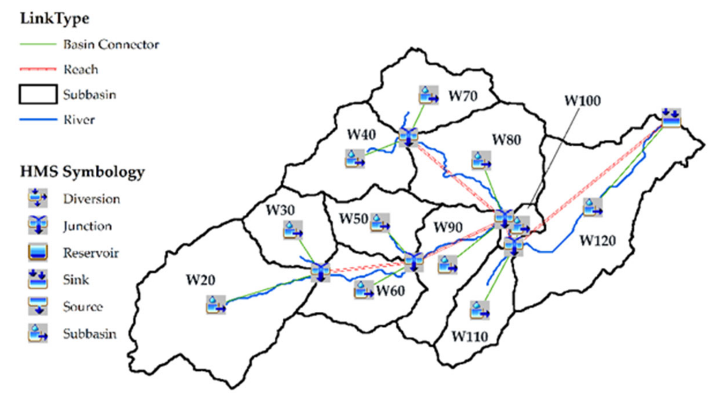
2.1. Study Area
2.2. Data Set
2.2.1. Hydrometeorological Database

| Data Type | Temporal Resolution | Spatial Resolution | Source | Reference |
|---|---|---|---|---|
| Precipitation gauge data | 1 h (2014–2020) | - | Local meteorological agencies | |
| Discharge data | 1 h (2014–2020) | - | Local meteorological agencies | |
| IMERG-Final data | 0.5 h (2014–2020) | 0.1 × 0.1° | https://disc.gsfc.nasa.gov/ (accessed on 23 August 2020) | [43] |
| DEM | - | 30 × 30 m | http://www.gscloud.cn (accessed on 5 July 2020) | |
| Landuse | - | 1 × 1 km | https://www.resdc.cn/DOI/ (accessed on 5 July 2020) | |
| Soil | - | 1 × 1 km | FAO, HWSD | [44] |
2.2.2. Physiographic Databases
3. Methodology
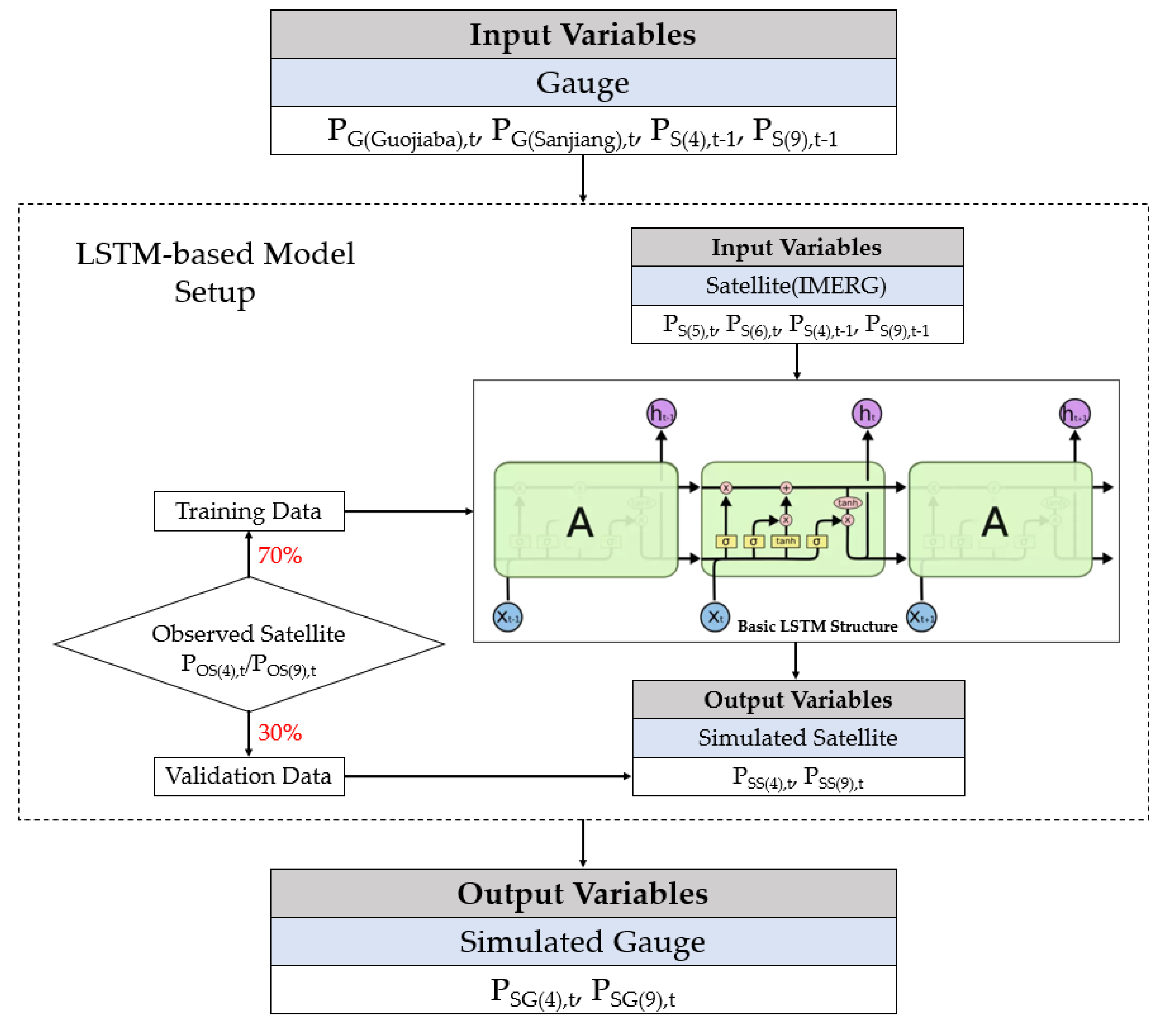
3.1. LSTM-Based Satellite-Gauge Merging Method

- (1)
- Parameter Setting
- (2)
- Training and Validation
- (3)
- Output Merged Data
3.2. Hydrological Model
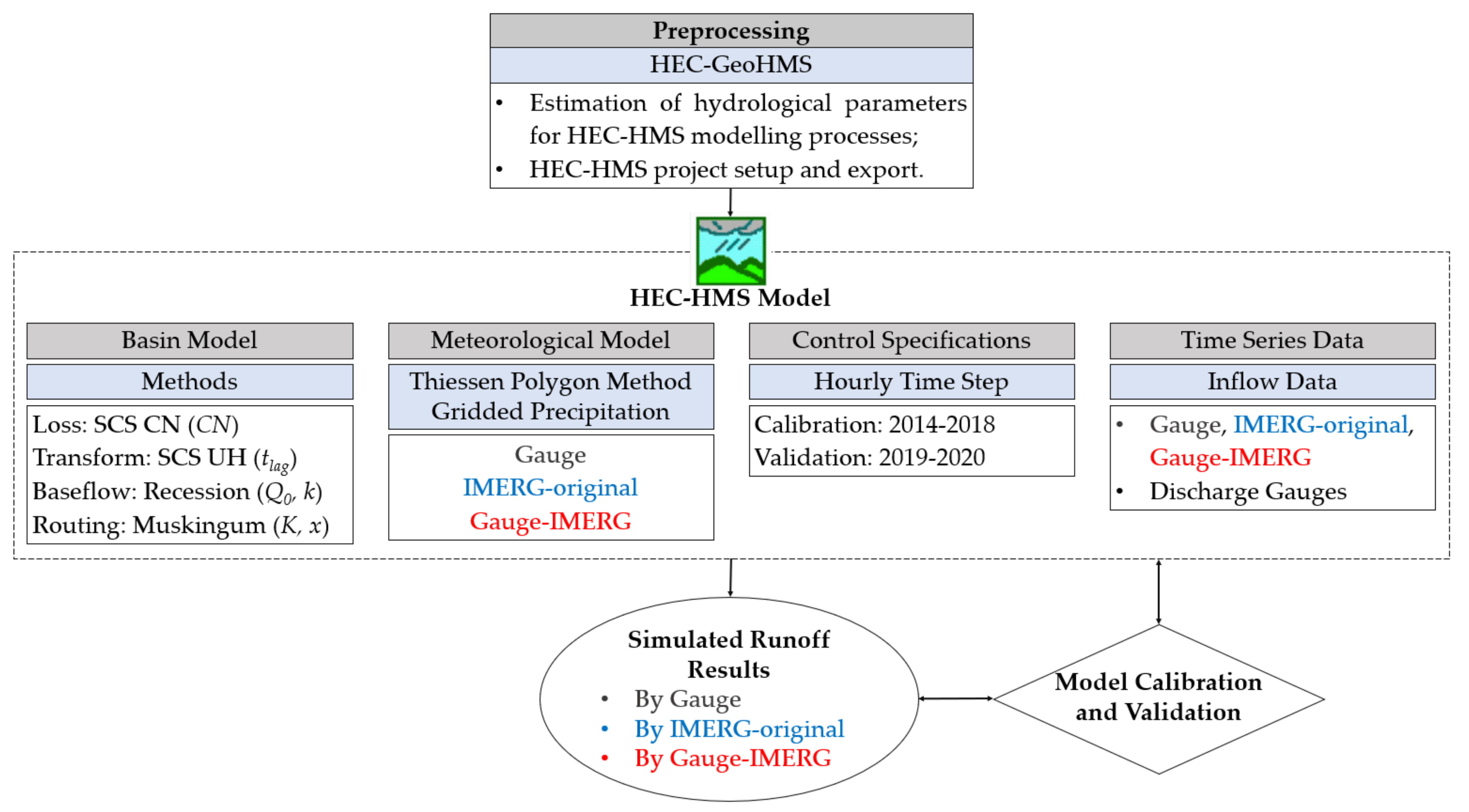
3.2.1. Preprocessing
3.2.2. Model Setup
- (1)
- Basin Model
- (2)
- Meteorological Model
- (3)
- Control Specifications
- (4)
- Time Series Data
3.2.3. Model Calibration and Validation
3.2.4. Model Evaluation
4. Results
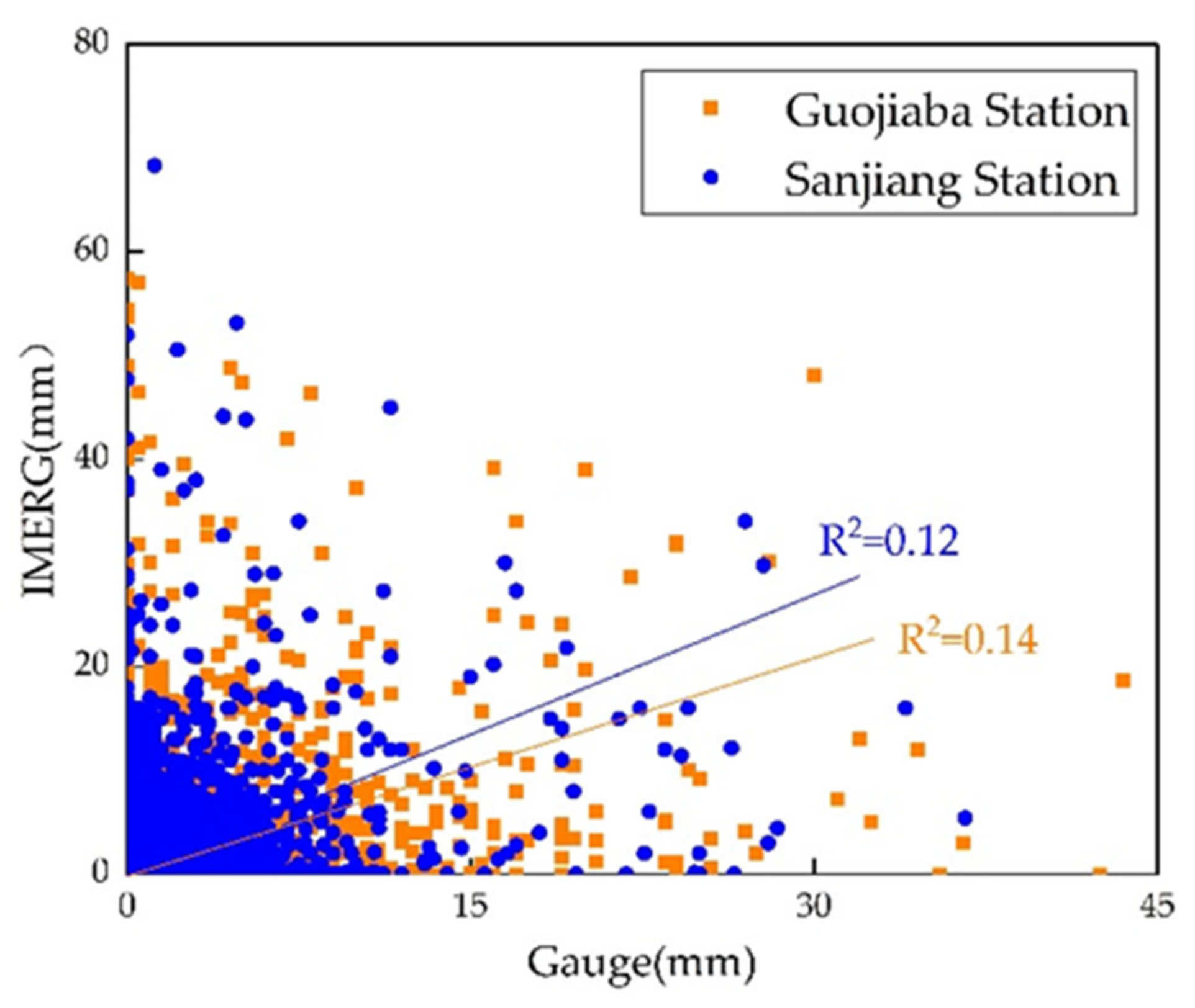
4.1. Accuracy Evaluation of Satellite Precipitation
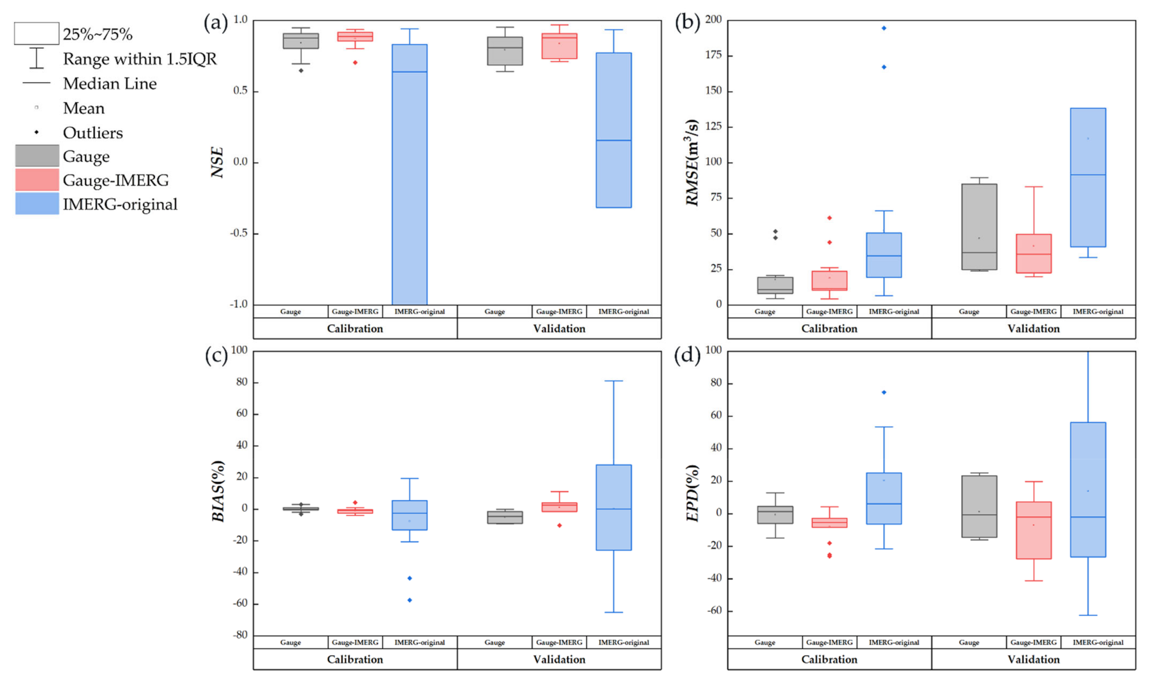
4.2. Overall Performance of Different Precipitation Data for Flood Simulation
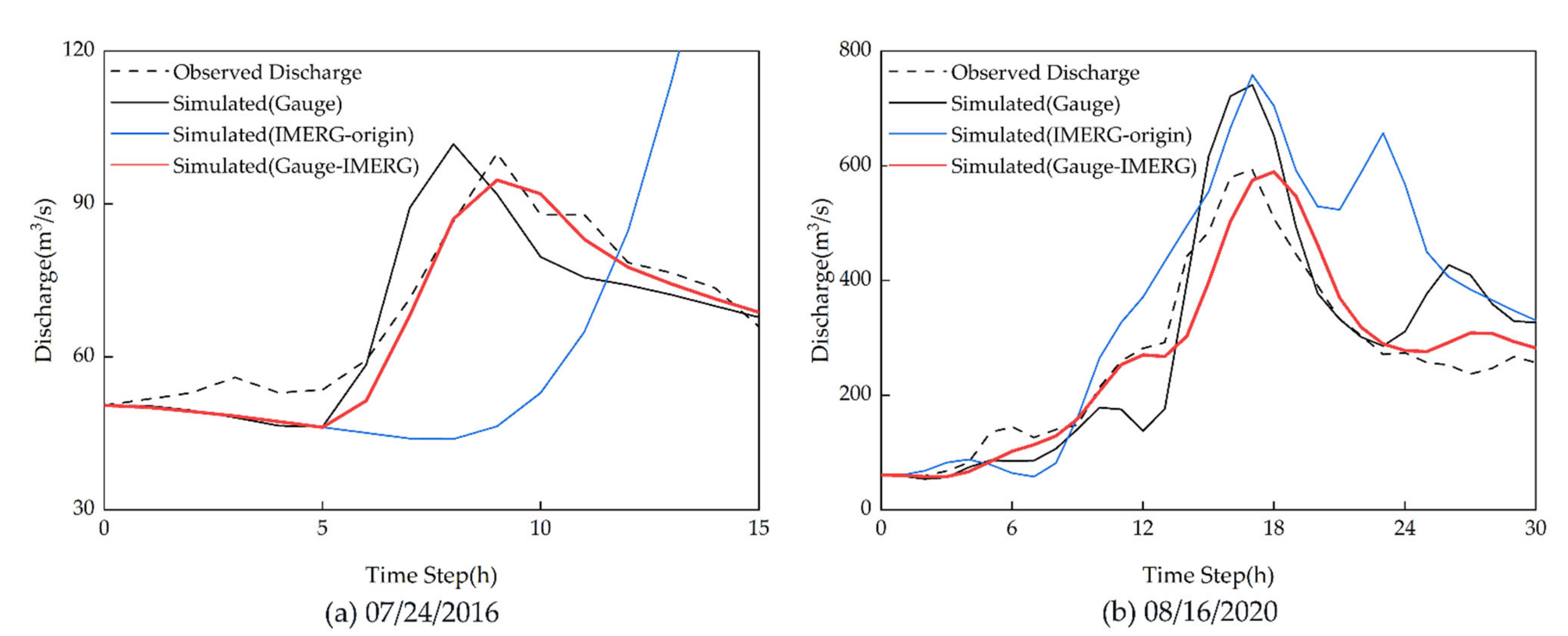
4.3. Performance Assessment of Typical Flood Events Simulation
5. Discussion
5.1. Validating the LSTM-Based Satellite-Gauge Merging Method
5.2. Uncertainties of Satellite Precipitation Products (SPPs) over Complex Terrains
6. Conclusions
Author Contributions
Funding
Institutional Review Board Statement
Informed Consent Statement
Data Availability Statement
Acknowledgments
Conflicts of Interest
References
- Kleinen, T.; Petschel-Held, G. Integrated assessment of changes in flooding probabilities due to climate change. Clim. Chang. 2007, 81, 283–312. [Google Scholar] [CrossRef]
- Todini, E. Flood Forecasting and Decision Making in the new Millennium. Where are We? Water Resour. Manag. 2017, 31, 3111–3129. [Google Scholar] [CrossRef]
- Beniston, M. Trends in joint quantiles of temperature and precipitation in Europe since 1901 and projected for 2100. Geophys. Res. Lett. 2009, 36. [Google Scholar] [CrossRef] [Green Version]
- Borga, M.; Anagnostou, E.N.; Blöschl, G.; Creutin, J.D. Flash flood forecasting, warning and risk management: The HYDRATE project. Environ. Sci. Policy 2011, 14, 834–844. [Google Scholar] [CrossRef]
- Norbiato, D.; Borga, M.; Dinale, R. Flash flood warning in ungauged basins by use of the flash flood guidance and model-based runoff thresholds. Meteorol. Appl. 2009, 16, 65–75. [Google Scholar] [CrossRef]
- Gebregiorgis, A.S.; Hossain, F. Understanding the Dependence of Satellite Rainfall Uncertainty on Topography and Climate for Hydrologic Model Simulation. IEEE Trans. Geosci. Remote Sens. 2013, 51, 704–718. [Google Scholar] [CrossRef]
- Sangati, M.; Borga, M.; Rabuffetti, D.; Bechini, R. Influence of rainfall and soil properties spatial aggregation on extreme flash flood response modelling: An evaluation based on the Sesia river basin, North Western Italy. Adv. Water Resour. 2009, 32, 1090–1106. [Google Scholar] [CrossRef]
- Viglione, A.; Chirico, G.B.; Woods, R.; Blöschl, G. Generalised synthesis of space–time variability in flood response: An analytical framework. J. Hydrol. 2010, 394, 198–212. [Google Scholar] [CrossRef]
- Levizzani, V.; Kidd, C.; Aonashi, K.; Bennartz, R.; Ferraro, R.R.; Huffman, G.J.; Roca, R.; Turk, F.J.; Wang, N.Y. The activities of the international precipitation working group. Q. J. R. Meteorol. Soc. 2018, 144, 3–15. [Google Scholar] [CrossRef] [Green Version]
- Sungmin, O.; Kirstetter, P.E. Evaluation of diurnal variation of GPM IMERG-derived summer precipitation over the contiguous US using MRMS data. Q. J. R. Meteorol. Soc. 2018, 144, 270–281. [Google Scholar] [CrossRef] [Green Version]
- Zoccatelli, D.; Borga, M.; Zanon, F.; Antonescu, B.; Stancalie, G. Which rainfall spatial information for flash flood response modelling? A numerical investigation based on data from the Carpathian range, Romania. J. Hydrol. 2010, 394, 148–161. [Google Scholar] [CrossRef]
- Kidd, C.; Levizzani, V. Status of satellite precipitation retrievals. Hydrol. Earth Syst. Sci. 2011, 15, 1109–1116. [Google Scholar] [CrossRef] [Green Version]
- Wang, H.; Wang, L.; He, J.; Ge, F.; Chen, Q.; Tang, S.; Yao, S. Can the GPM IMERG Hourly Products Replicate the Variation in Precipitation During the Wet Season Over the Sichuan Basin, China? Earth Space Sci. 2020, 7, e2020EA001090. [Google Scholar] [CrossRef] [Green Version]
- Mishra, V.; Shah, R.D. Development of an Experimental Near-Real-Time Drought Monitor for India. J. Hydrometeorol. 2015, 16, 327–345. [Google Scholar] [CrossRef]
- Mekonnen, K.; Melesse, A.M.; Woldesenbet, T.A. Spatial evaluation of satellite-retrieved extreme rainfall rates in the Upper Awash River Basin, Ethiopia. Atmos. Res. 2021, 249, 105297. [Google Scholar] [CrossRef]
- Solakian, J.; Maggioni, V.; Godrej, A.N. On the Performance of Satellite-Based Precipitation Products in Simulating Streamflow and Water Quality During Hydrometeorological Extremes. Front. Environ. Sci. 2020, 8, 585451. [Google Scholar] [CrossRef]
- Soo, E.Z.X.; Wan Jaafar, W.Z.; Lai, S.H.; Othman, F.; Elshafie, A.; Islam, T.; Srivastava, P.; Othman Hadi, H.S. Precision of raw and bias-adjusted satellite precipitation estimations (TRMM, IMERG, CMORPH, and PERSIANN) over extreme flood events: Case study in Langat river basin, Malaysia. J. Water Clim. Chang. 2020, 11, 322–342. [Google Scholar] [CrossRef]
- Zhu, B.; Huang, Y.; Zhang, Z.; Kong, R.; Tian, J.; Zhou, Y.; Chen, S.; Duan, Z. Evaluation of TMPA Satellite Precipitation in Driving VIC Hydrological Model over the Upper Yangtze River Basin. Water 2020, 12, 3230. [Google Scholar] [CrossRef]
- Zema, D.A.; Labate, A.; Martino, D.; Zimbone, S.M. Comparing Different Infiltration Methods of the HEC-HMS Model: The Case Study of the Mésima Torrent (Southern Italy). Land Degrad. Dev. 2016, 28, 294–308. [Google Scholar] [CrossRef]
- Zhou, L.; Rasmy, M.; Takeuchi, K.; Koike, T.; Selvarajah, H.; Ao, T. Adequacy of Near Real-Time Satellite Precipitation Products in Driving Flood Discharge Simulation in the Fuji River Basin, Japan. Appl. Sci. 2021, 11, 1087. [Google Scholar] [CrossRef]
- Habib, E.; Haile, A.; Sazib, N.; Zhang, Y.; Rientjes, T. Effect of Bias Correction of Satellite-Rainfall Estimates on Runoff Simulations at the Source of the Upper Blue Nile. Remote Sens. 2014, 6, 6688–6708. [Google Scholar] [CrossRef] [Green Version]
- Tian, Y.; Peters-Lidard, C.D.; Eylander, J.B. Real-Time Bias Reduction for Satellite-Based Precipitation Estimates. J. Hydrometeorol. 2010, 11, 1275–1285. [Google Scholar] [CrossRef]
- Borga, M.; Tonelli, F.; Moore, R.J.; Andrieu, H. Long-term assessment of bias adjustment in radar rainfall estimation. Water Resour. Res. 2002, 38, 8-1–8-10. [Google Scholar] [CrossRef] [Green Version]
- Ren, P.; Li, J.; Feng, P.; Guo, Y.; Ma, Q. Evaluation of Multiple Satellite Precipitation Products and Their Use in Hydrological Modelling over the Luanhe River Basin, China. Water 2018, 10, 677. [Google Scholar] [CrossRef] [Green Version]
- Zhang, L.; Li, X.; Zheng, D.; Zhang, K.; Ma, Q.; Zhao, Y.; Ge, Y. Merging multiple satellite-based precipitation products and gauge observations using a novel double machine learning approach. J. Hydrol. 2021, 594, 125969. [Google Scholar] [CrossRef]
- Shen, C. A Transdisciplinary Review of Deep Learning Research and Its Relevance for Water Resources Scientists. Water Resour. Res. 2018, 54, 8558–8593. [Google Scholar] [CrossRef]
- Kumar, D.; Singh, A.; Samui, P.; Jha, R.K. Forecasting monthly precipitation using sequential modelling. Hydrol. Sci. J. 2019, 64, 690–700. [Google Scholar] [CrossRef]
- Oshri, B.; Hu, A.; Adelson, P.; Chen, X.; Dupas, P.; Weinstein, J.; Burke, M.; Lobell, D.; Ermon, S. Infrastructure Quality Assessment in Africa using Satellite Imagery and Deep Learning. In Proceedings of the 24th ACM SIGKDD International Conference on Knowledge Discovery & Data Mining, London, UK, 19–23 August 2018; pp. 616–625. [Google Scholar]
- Tao, Y.M.; Gao, X.G.; Hsu, K.L.; Sorooshian, S.; Ihler, A. A Deep Neural Network Modeling Framework to Reduce Bias in Satellite Precipitation Products. J. Hydrometeorol. 2016, 17, 931–945. [Google Scholar] [CrossRef]
- Wu, H.; Yang, Q.; Liu, J.; Wang, G. A spatiotemporal deep fusion model for merging satellite and gauge precipitation in China. J. Hydrol. 2020, 584, 124664. [Google Scholar] [CrossRef]
- Wang, X.; Li, B.; Chen, Y.; Guo, H.; Wang, Y.; Lian, L. Applicability Evaluation of Multisource Satellite Precipitation Data for Hydrological Research in Arid Mountainous Areas. Remote Sens. 2020, 12, 2886. [Google Scholar] [CrossRef]
- Derin, Y.; Anagnostou, E.; Berne, A.; Borga, M.; Boudevillain, B.; Buytaert, W.; Chang, C.-H.; Chen, H.; Delrieu, G.; Hsu, Y.; et al. Evaluation of GPM-era Global Satellite Precipitation Products over Multiple Complex Terrain Regions. Remote Sens. 2019, 11, 2936. [Google Scholar] [CrossRef] [Green Version]
- Freitas, E.d.S.; Coelho, V.H.R.; Xuan, Y.; Melo, D.d.C.D.; Gadelha, A.N.; Santos, E.A.; Galvão, C.d.O.; Ramos Filho, G.M.; Barbosa, L.R.; Huffman, G.J.; et al. The performance of the IMERG satellite-based product in identifying sub-daily rainfall events and their properties. J. Hydrol. 2020, 589, 125128. [Google Scholar] [CrossRef]
- Wang, S.; Liu, J.; Wang, J.; Qiao, X.; Zhang, J. Evaluation of GPM IMERG V05B and TRMM 3B42V7 Precipitation Products over High Mountainous Tributaries in Lhasa with Dense Rain Gauges. Remote Sens. 2019, 11, 2080. [Google Scholar] [CrossRef] [Green Version]
- Bhatti, H.A.; Rientjes, T.; Haile, A.T.; Habib, E.; Verhoef, W. Evaluation of Bias Correction Method for Satellite-Based Rainfall Data. Sensors 2016, 16, 884. [Google Scholar] [CrossRef] [PubMed] [Green Version]
- Anagnostou, E.N.; Nikolopoulos, E.I.; Ehsan Bhuiyan, M.A. Machine Learning–Based Blending of Satellite and Reanalysis Precipitation Datasets: A Multiregional Tropical Complex Terrain Evaluation. J. Hydrometeorol. 2019, 20, 2147–2161. [Google Scholar] [CrossRef]
- Peng, F.; Zhao, S.; Chen, C.; Cong, D.; Wang, Y.; Ouyang, H. Evaluation and comparison of the precipitation detection ability of multiple satellite products in a typical agriculture area of China. Atmos. Res. 2020, 236, 104814. [Google Scholar] [CrossRef]
- Bhuiyan, M.A.E.; Yang, F.; Biswas, N.K.; Rahat, S.H.; Neelam, T.J. Machine Learning-Based Error Modeling to Improve GPM IMERG Precipitation Product over the Brahmaputra River Basin. Forecasting 2020, 2, 14. [Google Scholar] [CrossRef]
- Ding, L.; Ma, L.; Li, L.; Liu, C.; Li, N.; Yang, Z.; Yao, Y.; Lu, H. A Survey of Remote Sensing and Geographic Information System Applications for Flash Floods. Remote Sens. 2021, 13, 1818. [Google Scholar] [CrossRef]
- He, J.; Zhang, K.; Liu, X.; Liu, G.; Zhao, X.; Xie, Z.; Lu, H. Vegetation restoration monitoring in Yingxiu landslide area after the 2008 Wenchuan earthquake. Earthq. Res. China 2020, 34, 157–166. [Google Scholar] [CrossRef]
- Lu, H.; Ma, L.; Fu, X.; Liu, C.; Wang, Z.; Tang, M.; Li, N. Landslides Information Extraction Using Object-Oriented Image Analysis Paradigm Based on Deep Learning and Transfer Learning. Remote Sens. 2020, 12, 752. [Google Scholar] [CrossRef] [Green Version]
- Lo Conti, F.; Hsu, K.-L.; Noto, L.V.; Sorooshian, S. Evaluation and comparison of satellite precipitation estimates with reference to a local area in the Mediterranean Sea. Atmos. Res. 2014, 138, 189–204. [Google Scholar] [CrossRef] [Green Version]
- Huffman, G.J.; Stocker, E.F.; Bolvin, D.T.; Kelkin, E.J.; Tan, J. GPM IMERG Late Precipitation L3 1 Day 0.1 Degree×0.1 Degree V06; Andrey, S., Greenbelt, M.D., Eds.; Goddard Earth Sciences Data and Information Services Center (GES DISC): Washington, DC, USA, 2019. Available online: https://disc.gsfc.nasa.gov/datasets/GPM_3IMERGDF_06/summary (accessed on 1 May 2020).
- FAO/IIASA/ISRIC/ISS-CAS/JRC. Harmonized World Soil Database (Version 1.1); FAO: Rome, Italy; IIASA: Laxenburg, Austria, 2009; Available online: http://www.fao.org/3/a-aq361e.pdf (accessed on 1 May 2020).
- De Villiers, J.; Barnard, E. Backpropagation neural nets with one and two hidden layers. IEEE Trans. Neural Netw. 1993, 4, 136–141. [Google Scholar] [CrossRef]
- Hornik, K.; Stinchcombe, M.; White, H. Multilayer Feedforward Networks Are Universal Approximators. Neural Netw. 1989, 2, 359–366. [Google Scholar] [CrossRef]
- Cheng, X.; Ma, X.; Wang, W.; Xiao, Y.; Wang, Q.; Liu, X. Application of HEC-HMS Parameter Regionalization in Small Watershed of Hilly Area. Water Resour. Manag. 2021, 35, 1961–1976. [Google Scholar] [CrossRef]
- El Hassan, A.A.; Sharif, H.O.; Jackson, T.; Chintalapudi, S. Performance of a conceptual and physically based model in simulating the response of a semi-urbanized watershed in San Antonio, Texas. Hydrol. Process. 2013, 27, 3394–3408. [Google Scholar] [CrossRef]
- Bai, Y.; Zhang, Z.; Zhao, W. Assessing the Impact of Climate Change on Flood Events Using HEC-HMS and CMIP5. Water Air Soil Pollut. 2019, 230, 119. [Google Scholar] [CrossRef]
- Mohammadi Hashemi, M.; Saghafian, B.; Zakeri Niri, M.; Najarchi, M. Applicability of Rainfall–Runoff Models in Two Simplified Watersheds. Iran. J. Sci. Technol. Trans. Civ. Eng. 2021. [Google Scholar] [CrossRef]
- Hussain, F.; Wu, R.-S.; Yu, K.-C. Application of Physically Based Semi-Distributed Hec-Hms Model for Flow Simulation in Tributary Catchments of Kaohsiung Area Taiwan. J. Mar. Sci. Technol. 2021, 29, 4. [Google Scholar] [CrossRef]
- Belayneh, A.; Sintayehu, G.; Gedam, K.; Muluken, T. Evaluation of satellite precipitation products using HEC-HMS model. Model. Earth Syst. Environ. 2020, 6, 2015–2032. [Google Scholar] [CrossRef]
- Kazezyılmaz-Alhan, C.M.; Yalçın, İ.; Javanshour, K.; Aytekin, M.; Gülbaz, S. A hydrological model for Ayamama watershed in Istanbul, Turkey, using HEC-HMS. Water Pract. Technol. 2021, 16, 154–161. [Google Scholar] [CrossRef]
- Gilewski, P.; Nawalany, M. Inter-Comparison of Rain-Gauge, Radar, and Satellite (IMERG GPM) Precipitation Estimates Performance for Rainfall-Runoff Modeling in a Mountainous Catchment in Poland. Water 2018, 10, 1665. [Google Scholar] [CrossRef] [Green Version]
- Baez-Villanueva, O.M.; Zambrano-Bigiarini, M.; Beck, H.E.; McNamara, I.; Ribbe, L.; Nauditt, A.; Birkel, C.; Verbist, K.; Giraldo-Osorio, J.D.; Xuan Thinh, N. RF-MEP: A novel Random Forest method for merging gridded precipitation products and ground-based measurements. Remote Sens. Environ. 2020, 239, 111606. [Google Scholar] [CrossRef]
- Mei, Y.; Nikolopoulos, E.I.; Anagnostou, E.N.; Borga, M. Evaluating Satellite Precipitation Error Propagation in Runoff Simulations of Mountainous Basins. J. Hydrometeorol. 2016, 17, 1407–1423. [Google Scholar] [CrossRef]


| Area (km2) | Elevation (m) | River Slope (°) | ||||
|---|---|---|---|---|---|---|
| Maximum | Minimum | Average | Maximum | Minimum | Average | |
| 600.4 | 4897.0 | 774.0 | 2174.8 | 87.2 | 0 | 31.4 |
| Station | Evaluation Criteria | ||
|---|---|---|---|
| CC | RMSE | BIAS | |
| Guojiaba | 0.36 | 1.45 | 0.09 |
| Sanjiang | 0.51 | 1.58 | 0.1 |
| Statistical Indicators | Gauge | IMERG-Original | Gauge-IMERG | ||||
|---|---|---|---|---|---|---|---|
| Calibration | Validation | Calibration | Validation | Calibration | Validation | ||
| NSE | Mean | 0.84 | 0.80 | −1.22 | −1.33 | 0.87 | 0.84 |
| Lower quartile | 0.81 | 0.72 | −2.31 | −0.13 | 0.86 | 0.75 | |
| Median | 0.88 | 0.81 | 0.64 | 0.16 | 0.89 | 0.88 | |
| Upper quartile | 0.91 | 0.86 | 0.83 | 0.57 | 0.92 | 0.90 | |
| Range | [0.65, 0.95] | [0.64, 0.95] | [−9.72, 0.94] | [−11.26, 0.94] | [0.7, 0.94] | [0.71, 0.97] | |
| RMSE (m3/s) | Mean | 17.84 | 46.83 | 52.40 | 116.95 | 19.04 | 41.67 |
| Lower quartile | 8.14 | 25.28 | 19.58 | 50.39 | 10.47 | 27.92 | |
| Median | 11.01 | 36.87 | 34.59 | 91.48 | 11.51 | 35.68 | |
| Upper quartile | 19.51 | 63.34 | 50.71 | 134.83 | 23.74 | 48.59 | |
| Range | [4.54, 51.75] | [24.07, 89.64] | [6.68, 194.71] | [33.39, 323.31] | [4.26, 61.37] | [19.85, 83.14] | |
| BIAS (%) | Mean | 0.2% | −4.8% | −7.6% | 0.5% | −0.9% | 1.3% |
| Lower quartile | −0.5% | −7.8% | −13.1% | −20.9% | −2.5% | −0.7% | |
| Median | −0.1% | −4.5% | −2.5% | 0.2% | −0.7% | 2.5% | |
| Upper quartile | 0.9% | −2.0% | 5.5% | 14.5% | −0.2% | 3.4% | |
| Range | [−3.0%, 3.1%] | [−9.3%, −0.1%] | [−57.4%, 19.5%] | [−65.2%, 81.2%] | [−3.8%, 4.3%] | [−10.2%, 11.1%] | |
| EPD (%) | Mean | −0.6% | 1.4% | 20.5% | 14.0% | −7.8% | −6.9% |
| Lower quartile | −5.9% | −13.5% | −6.3% | −17.2% | −8.3% | −15.8% | |
| Median | 1.4% | −0.6% | 6.0% | −2.0% | −5.3% | −1.9% | |
| Upper quartile | 4.6% | 14.2% | 25.2% | 42.1% | −2.7% | 3.4% | |
| Range | [−14.9%, 12.8%] | [−16.0%, 25.5%] | [−21.5%, 117.7%] | [−62.3%, 112.3%] | [−26.0%, 4.4%] | [−41.1%, 19.8%] | |
| Events | NSE | RMSE (m3/s) | BIAS (%) | EPD (%) | ||||||||
|---|---|---|---|---|---|---|---|---|---|---|---|---|
| Gauge | IMERG-Original | Gauge-IMERG | Gauge | IMERG-Original | Gauge-IMERG | Gauge | IMERG-Original | Gauge-IMERG | Gauge | IMERG-Original | Gauge-IMERG | |
| 12 September 2014 | 0.81 | 0.46 | 0.80 | 10.62 | 19.58 | 11.51 | −1.5% | 19.2% | −3.8% | 3.6% | −21.5% | 0.3% |
| 22 September 2015 | 0.77 | 0.75 | 0.90 | 6.50 | 6.68 | 4.26 | 0.8% | −2.5% | −0.5% | 1.4% | 3.5% | −3.8% |
| 14 July 2016 | 0.93 | 0.94 | 0.94 | 11.01 | 10.05 | 10.47 | 0.2% | 5.5% | −3.8% | 4.6% | −8.0% | 1.8% |
| 24 July 2016 | 0.70 | −5.92 | 0.92 | 8.14 | 40.65 | 4.49 | 3.1% | −0.5% | 4.3% | 1.8% | 74.7% | −5.3% |
| 26 July 2016 | 0.88 | −9.72 | 0.80 | 20.85 | 194.71 | 26.33 | −3.0% | −57.4% | 1.0% | −14.9% | 117.7% | −25.1% |
| 4 August 2017 | 0.95 | 0.51 | 0.93 | 7.85 | 35.31 | 13.83 | 3.0% | −20.6% | 0.9% | −1.7% | 14.5% | −8.3% |
| 25 August 2017 | 0.91 | 0.75 | 0.88 | 19.51 | 34.59 | 23.74 | 2.1% | 8.2% | −1.3% | 11.2% | 22.2% | −17.9% |
| 28 August 2017 | 0.89 | 0.83 | 0.86 | 47.23 | 66.20 | 61.37 | 0.9% | −12.2% | −0.7% | −14.7% | 1.5% | −26.0% |
| 9 July 2018 | 0.84 | 0.64 | 0.92 | 15.54 | 22.68 | 10.70 | −0.5% | −13.1% | −0.4% | 6.4% | 25.2% | 4.4% |
| 10 July 2018 | 0.89 | −2.31 | 0.88 | 4.54 | 24.48 | 4.64 | −0.1% | 19.5% | −0.2% | −0.4% | −17.0% | −2.7% |
| 11 July 2018 | 0.93 | −4.50 | 0.91 | 19.01 | 167.38 | 21.05 | −0.1% | −43.5% | −3.5% | −5.9% | 53.4% | −7.8% |
| 19 July 2018 | 0.65 | 0.84 | 0.70 | 9.45 | 8.18 | 10.90 | −1.9% | −2.8% | −2.5% | 12.8% | 6.0% | −3.6% |
| 20 July 2018 | 0.82 | 0.85 | 0.89 | 51.75 | 50.71 | 44.16 | −0.1% | 1.5% | −1.0% | −11.9% | −6.3% | −7.8% |
| 21 August 2019 | 0.81 | 0.16 | 0.88 | 41.58 | 91.48 | 35.68 | −6.8% | −15.9% | 2.5% | −14.5% | 56.2% | −1.9% |
| 22 August 2019 | 0.88 | 0.36 | 0.91 | 24.07 | 59.82 | 22.71 | −0.1% | 28.1% | 2.7% | −0.6% | −26.5% | 7.4% |
| 26 June 2020 | 0.95 | −0.32 | 0.97 | 24.84 | 131.28 | 19.85 | −1.5% | 81.2% | 0.1% | −12.6% | −62.3% | −4.0% |
| 7 August 2020 | 0.76 | −11.26 | 0.71 | 36.87 | 323.31 | 49.68 | −8.9% | −65.2% | 11.1% | −16.0% | 112.3% | −41.1% |
| 12 August 2020 | 0.84 | 0.77 | 0.78 | 25.71 | 33.39 | 33.12 | −2.5% | 0.2% | 4.1% | 4.9% | −2.0% | −27.7% |
| 16 August 2020 | 0.64 | 0.05 | 0.89 | 85.09 | 138.37 | 47.50 | −9.3% | −25.9% | −1.4% | 25.0% | 27.9% | −0.6% |
| 31 August 2020 | 0.69 | 0.94 | 0.73 | 89.64 | 40.96 | 83.14 | −4.5% | 0.9% | −10.2% | 23.4% | −7.8% | 19.8% |
| Events | Precipitation Inputs | Error of Time to Peak (h) | Peak Disch (m3/s) | NSE | RMSE (m3/s) | BIAS | EPD |
|---|---|---|---|---|---|---|---|
| 24 July 2016 | Gauge | 1 | 101.8 | 0.70 | 8.14 | 3.1% | 1.8% |
| IMERG-origin | 6 | 174.7 | −5.92 | 40.65 | −0.5% | 74.7% | |
| Gauge-IMERG | 0 | 94.7 | 0.92 | 4.49 | 4.3% | −5.3% | |
| Gauge | 0 | 741.3 | 0.64 | 85.09 | −9.3% | 25.0% | |
| 16 August 2020 | IMERG-origin | 0 | 758.7 | 0.05 | 138.37 | −25.9% | 27.9% |
| Gauge-IMERG | 1 | 589.7 | 0.89 | 47.50 | −1.4% | −0.6% |
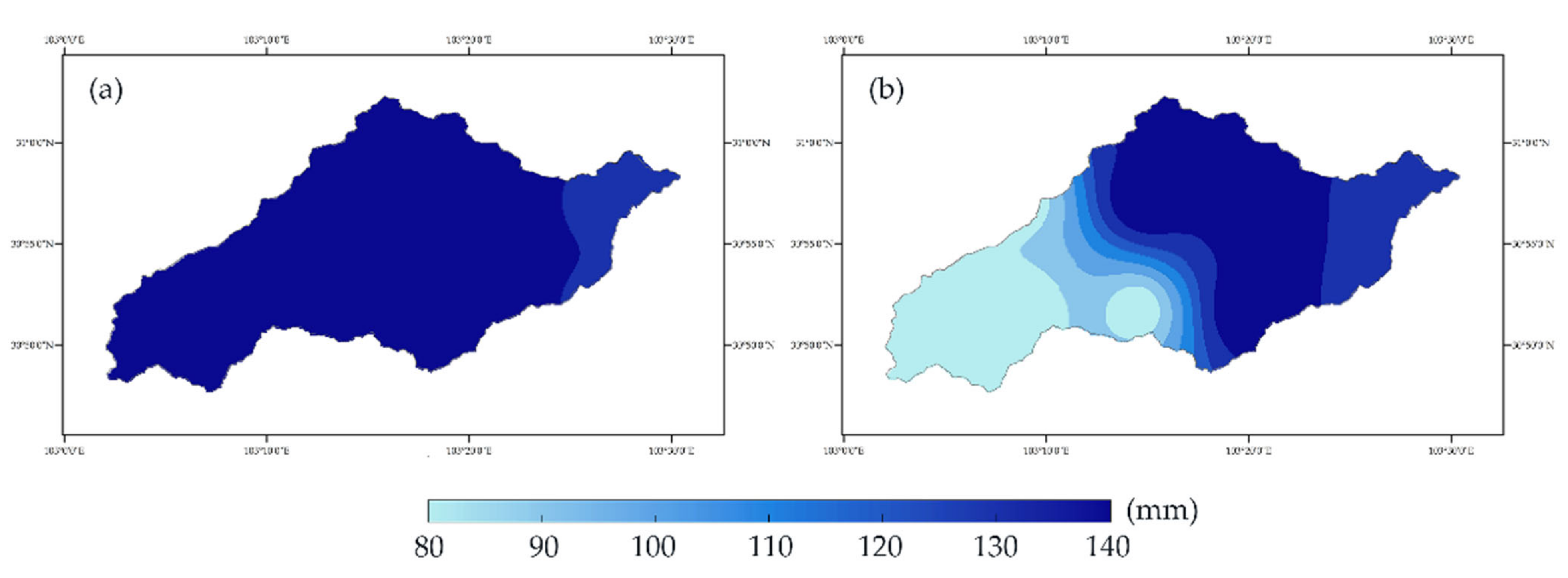
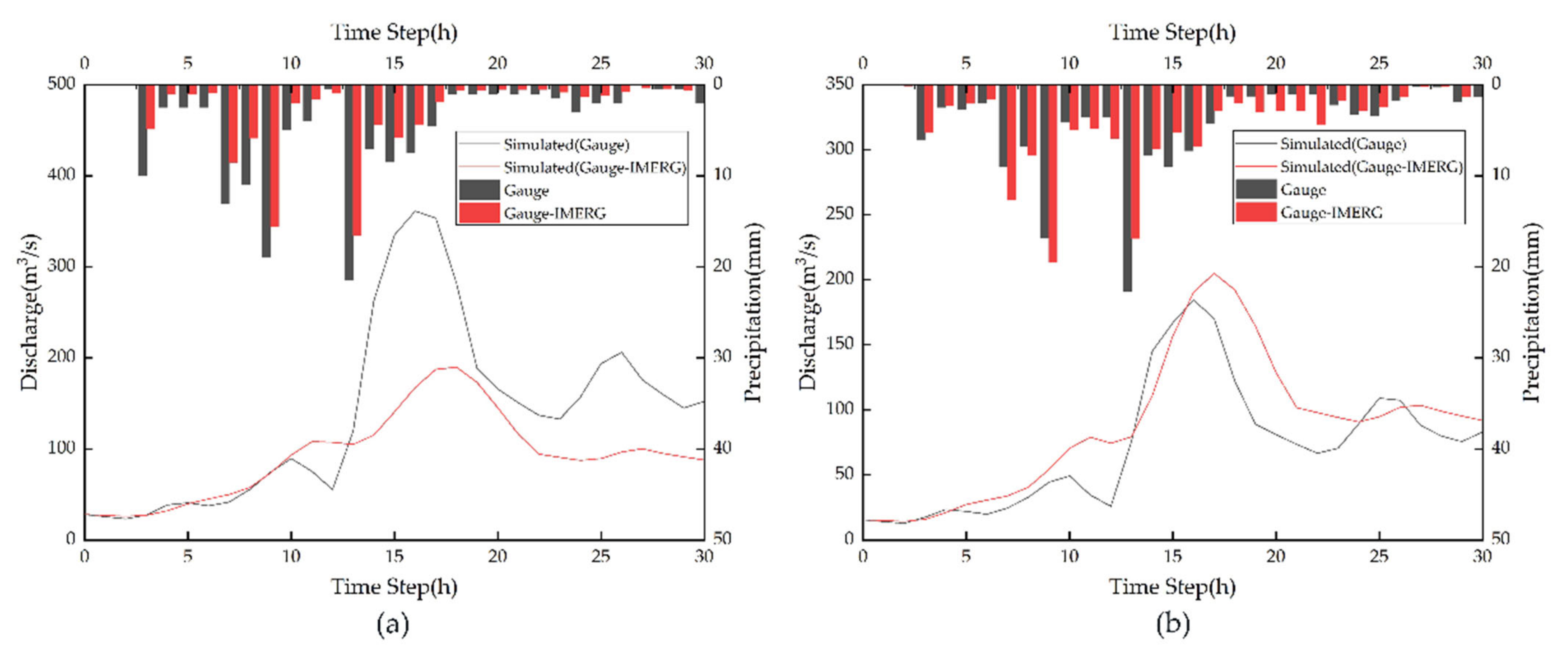
| Type of Inputs | Precipitation Amount (mm) | Discharge | ||||
|---|---|---|---|---|---|---|
| Peak Discharge (m3/s) | Peak Time (h) | |||||
| Upstream | Downstream | Upstream | Downstream | Upstream | Downstream | |
| Gauge | 136 | 128 | 361.3 | 184.7 | 16 | 16 |
| Gauge-IMERG | 84.4 | 131.9 | 189.8 | 205.1 | 18 | 17 |
Publisher’s Note: MDPI stays neutral with regard to jurisdictional claims in published maps and institutional affiliations. |
© 2021 by the authors. Licensee MDPI, Basel, Switzerland. This article is an open access article distributed under the terms and conditions of the Creative Commons Attribution (CC BY) license (https://creativecommons.org/licenses/by/4.0/).
Share and Cite
Tang, X.; Yin, Z.; Qin, G.; Guo, L.; Li, H. Integration of Satellite Precipitation Data and Deep Learning for Improving Flash Flood Simulation in a Poor-Gauged Mountainous Catchment. Remote Sens. 2021, 13, 5083. https://doi.org/10.3390/rs13245083
Tang X, Yin Z, Qin G, Guo L, Li H. Integration of Satellite Precipitation Data and Deep Learning for Improving Flash Flood Simulation in a Poor-Gauged Mountainous Catchment. Remote Sensing. 2021; 13(24):5083. https://doi.org/10.3390/rs13245083
Chicago/Turabian StyleTang, Xuan, Zhaorui Yin, Guanghua Qin, Li Guo, and Hongxia Li. 2021. "Integration of Satellite Precipitation Data and Deep Learning for Improving Flash Flood Simulation in a Poor-Gauged Mountainous Catchment" Remote Sensing 13, no. 24: 5083. https://doi.org/10.3390/rs13245083