Reducing Scaling Effect on Downscaled Land Surface Temperature Maps in Heterogenous Urban Environments

Abstract

The literature review indicates that a scaling effect does exist in downscaling land surface temperature (DLST) processes, and no substantial methods were specially developed for addressing it. In this research, the main aim is to develop a new method to reduce the scaling effect on DLST maps at high resolutions. A thermal component-based thermal spectral unmixing (TSU) model was modified and a multiple regression (REG) model was adopted to create DLST maps at high resolutions. A combined variance of red and NIR bands at a very high resolution with a difference image between upscaled LST and DLST was used to develop a new method. With two case data sets, LSTs at coarse resolutions were downscaled by using the modified TSU model and the REG model to create DLST results. The new method with a correction term expression (a linear model created by using a semi-empirical approach) was used to improve the DLST maps in the two case study areas. The experimental results indicate that the new method could reduce the root mean square error and the mean absolute error >30% and >33%, respectively, and thus demonstrate that the proposed method was effective and significant, especially reducing the scaling effect on DLST results at very high resolutions. The novel significance for the new method is directly reducing the scaling effect on DLST maps at high resolutions.

1. Introduction

Many existing studies have proved that a scaling effect exists in downscaling the land surface temperature (DLST) processes, especially downscaling LST to high resolutions (e.g., [1,2]). In this research, the scaling effect is defined as the error in the downscaled LST at a target (high) resolution, which may be understood as a difference between DLST and true LST at high resolutions [2,3]. Given the fact that the error is caused by the LST-scaling factors relationship at the native resolution [3] and the spatial heterogeneity of landscapes in a study area [4,5], usually, the scaling effect (error) may increase with the refinement of the spatial resolution in downscaling LST processes. In practice, a basic assumption that relationships between LST and scaling factors are scale-invariant across different resolutions is debated and problematic [6,7]. In fact, the relationships between LST and scaling factors are spatially variable in various environments, as demonstrated by many investigators (e.g., [1,2,8,9,10]). For example, such a scale effect for an association of vegetation index with LST at different spatial resolutions was demonstrated by [8]. They proved that the relationship changed significantly across different resolutions due to the various heterogeneity of different spatial extents. Zhou et al. [2] demonstrated that the scaling effect relied on the values of biophysical descriptors (e.g., the phenology) and the scaling factors, and on the varying distribution probability of the LST across spatial resolutions. Ghosh and Joshi [9] also confirmed the spatial scaling effect, which depends on the characteristics of surface materials and cover types, and on regression models selected. In our latest work [1], our findings irrefutably demonstrate that the scaling effect in downscaling LST to higher resolutions is great and significant. In short, the scaling effect in downscaling LST processes does exist at high resolutions.

To improve downscaling LST from a relatively coarse resolution to a relatively high resolution, many researchers have developed various advanced DLST techniques and methods to compensate the scaling effect in DLST processes at higher resolutions. Generally, such methods and techniques may be classified into three categories: regression-based, machine-learning-based, and thermal spectral unmixing-based. The regression-based methods include linear and non-linear multivariate regression models (e.g., [1,3,8,9,11,12,13,14,15,16]). Usually, regression relationships between LST and scaling factors (predictors) within a scene are determined empirically at a coarse (thermal band) resolution and then applied to the fine (optical band) resolution to produce sharpened thermal band imagery. This category of methods is relatively easy to implement, and DLST results are satisfactorily accurate. However, the main limitations of this category are that regression correlations between LST and scaling factors might be insufficient for some regions [2] and significantly site specific [10].

The machine learning-based methods may include various artificial neural networks, support vector machines, random forest models, and partial least square models (e.g., [1,9,17,18,19,20]). They usually perform better compared to the regression-based methods and result in a high accuracy by fitting nonlinear relationships between LST and independent variables [21]. There are many advantages of different machine learning methods, e.g., nondeterministic reasoning with complex causality due to its self-learning, self-organization, error tolerance, and excellent nonlinear approximation ability of artificial neural networks; rapid processing of high-dimensional data with support vector machines; and insensitivity to multicollinearity of independent variables of random forest [21]. However, the major limitations of the most machine learning-based methods may include intensive computational resources, complex structure of algorithms, and a black box model, etc.

There are only a few thermal spectral unmixing (TSU)-based DLST methods in the existing literature (e.g., [22,23,24,25,26]). The TSU-based DLST methods can be described as follows: thermal component temperatures inside a pixel are decomposed based on multi-temporal, spatial, spectral, or angular observations [27]. The thermal component temperatures or radiances at an initial high resolution, created by solving the TSU model from coarse resolution thermal (or LST) data, can then be aggregated into different high resolution DLST maps. For example, Deng and Wu [23] proposed a VHR spectral unmixing and thermal mixing (VHR-SUTM) approach to downscale LST at a high resolution. The VHR-SUTM method consists of two key steps: (1) spectral unmixing with IKONOS data to obtain fractions of land cover types that respond to unique thermal characteristics, and (2) thermal unmixing with lower resolution LST data and corresponding land cover fractions to estimate per-pixel VHR LST values. Their unmixed results indicate that the resampled VHR LST estimates were highly consistent with the corresponding resolution of retrieved LSTs. Wang et al. [26] introduced the thermal component-based spectral unmixing technique to produce thermal component radiance. Their results indicate that downscaled LST could differentiate temperatures over major land types and capture both seasonal and diurnal LST dynamics. The technique is used for directly solving a system of linear spectral mixture models encoding the thermal component-LST (or thermal radiance) relationship at a coarse resolution, and then the solution is applied to a finer resolution to obtain high-resolution LST results. Thus, it is less time-consuming, even with a large downscaling factor of 30, and significantly outperforms classic downscaling techniques [26]. Given the advantages (easy to use and high accurate DLST results) of the TSU technique with thermal components extracted from high-resolution optical data and potential applications, we proposed to explore its potential by modifying the technique by directly using spectral clusters representing thermal components and fitting a thermal component-LST relationship to improve the DLST process in this study as well.

Compared to traditional DLST methods, such as DisTrad and TsHARP, all these advanced methods and techniques do improve LST downscaled accuracy and may reduce the scaling effect on DLST results to a certain extent. However, there still exists a certain degree of scaling effect in DLST processes, especially at high resolutions. After a relatively extensive literature review, limited by our knowledge, no techniques and methods are found for directly reducing the scaling effect on DLSTs results. Therefore, it is obvious for us that developing a new method to directly reduce the spatial scaling effect on DLST results, created by various advanced downscaling methods, is a direction to improve DLSTs at high resolutions. In addition, a DLST product at a high resolution with a lower (reduced) spatial scaling effect (error) is always beneficial to many application areas, such as high-resolution soil-moisture mapping [28,29].

According to the theory of temperature field, most current DLST processing methods and techniques are based on relatively steady-state two-dimensional temperature field and assume that the temperature field is continuous and smooth within a homogenous landscape (e.g., a water body or grassland), but over very heterogenous landscapes (e.g., an urban environment), the temperature field should be discrete and rough. However, for some spatiotemporal DLST methods, an unsteady-state three- (or four- in mountain areas) dimensional temperature field should be considered because the field depends on the temperatures on the two or three spatial coordinates and time. Therefore, in this study, the temperature field should be discrete and rough over heterogenous urban environments. Accordingly, developing a method to reduce the scaling effect on DLST results should consider the discrete and rough temperature field, induced by heterogenous landscapes.

In fact, some studies demonstrate that the scaling effect on DLST maps is related to the degree of heterogeneity of surface features/materials within pixels at specific resolutions. This issue was proved by Garrigues et al. [4,5] by quantifying the intra-pixel heterogeneity for mapping normalized difference vegetation index and leaf area index with moderate resolution remote sensing data and non-linear estimation processes. Garrigues et al. [30] also used a geostatistical linear model to quantify the landscape spatial heterogeneity with high-resolution red and NIR band images. Hu and Islam [31] demonstrated that the spatial heterogeneity of surface emittance, flux exchange and air temperature at a pixel level would introduce scaling-up errors of sensible heat flux in modeling remote sensing data. To study the effects of the spatial heterogeneity at a pixel level on scaling-up land surface parameters (e.g., leaf area index and evapotranspiration/soil moisture), Hu and Islam [32] proposed concepts of lumped model and distributed model in addressing the effects. According to [32], a lumped model representation assumes spatial homogeneity within a pixel, takes pixel-scale average parameters as the input and produces pixel-level output. A distributed model accounts for the spatial heterogeneity of parameters by dividing the pixel into a number of subpixels, and then the outputs from subpixels are aggregated by a suitable kernel to obtain the pixel-level output. They further used a small perturbation approach and added second-order correction terms to lumped model estimation to obtain distributed model output. In this study, we would develop a new method to address the effect of heterogeneity of surface features/materials within pixels at a specific resolution in DLST processes by introducing a correction term (CT) to reduce the scaling effect on DLST results. Note that the new method with a simulated CT is expected to correct the scaling effect on DLST results created by any advanced DLST methods. For this case, we referred to the basic concept and idea of the correction terms and their application in [32].

Therefore, the main aim of this study is to develop a new method to improve DLST results by reducing the spatial scaling effect on the DLST results by using the CT with a combined variance extracted from red and NIR high-resolution band images. The adoption of the red and NIR bands to construct the correction term was based on the literature review (e.g., [9,30,33]) and on the statistical results of the standard deviation (SD) of VNIR bands of the hyperspectral imagery used in this work (SDs of NIR and red bands were the largest and second largest among all VNIR bands). A modified thermal spectral unmixing (TSU) model with spectral clusters, which respond to thermal components, and a multiple regression (REG) model were utilized in downscaling LST processes. ASTER 90 m LST product and upscaled 100 m LST were downscaled to LSTs at finer resolutions. High-resolution DLSTs were validated with LSTs upscaled from the native 2 m pixel size. Overall, in this research, two specific objectives are pursued: (1) to test the performance of a modified TSU model with multi-spectral clusters to directly downscale LST to different high resolutions; (2) to develop and assess a new method with a CT to reduce the scaling effect on DLST results at high resolutions. The expected novel significances for this study include (1) directly downscaling LST with the modified TSU model and spectral clusters to obtain thermal components’ temperatures (different from the TSU model by Wang et al. [26], which downscales thermal radiance with land use/land cover types extracted from high-resolution optical data to obtain thermal components’ radiance), and (2) the newly developed method with the CT to significantly improve DLST results at high resolutions. Relevant issues related to spectral clusters responding thermal components and thermal physical characteristics, determining mask images and expression for running the CT, and limitations for the current CT expression are discussed. Some suggestions in further reducing the scaling effect on DLST results are also provided.

2. Study Areas and Data Sets

2.1. Study Areas

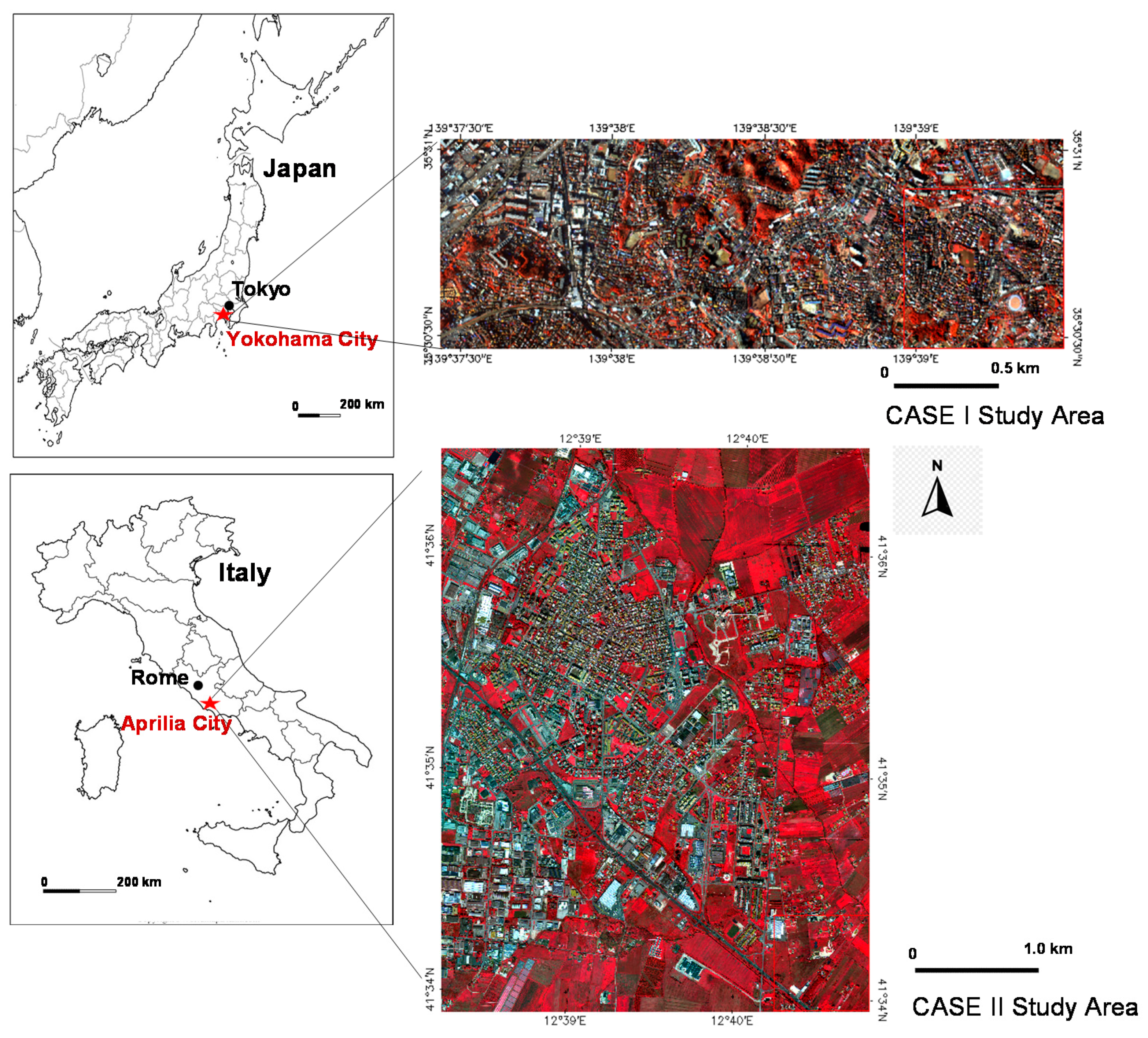
Two case study areas (CASEs I and II) were selected for this research because both areas have a heterogenous urban environment and available VHR TIR and optical data required for this research. The CASE I study area, located at approximately 35.3° N and 139.5° E, covers 1.1 × 3.1 km² and is within the City of Yokohama, Japan (Figure 1). There are over 3.7 million people in the city. The city has typical heterogenous urban environments including various man-made materials covering buildings, rooves, and road surfaces. There are also relatively fewer vegetated areas (parks, lawns/turfs), bare soil areas, and water bodies in the area. Yokohama features a humid subtropical climate with hot, humid summers and chilly winters with a yearly average temperature of 16.2 °C (April and May average: 16.7 °C) and yearly precipitation of 1730.8 mm (April and May monthly average: 147.9 mm) [34]. The CASE II study area is located at approximately 41.35° N and 12.39° E and comprises the City of Aprilia, near Rome, Central Italy (Figure 1). The selected area has 4.7 × 3.5 km² with a total population of 73 k. The CASE II study area is covered by typical residential, industrial estates, rural, and vegetated areas. The city has a Mediterranean climate with hot, dry summers and mild, humid winters with a yearly average temperature of 19.0 °C (March average 13.0 °C) and yearly precipitation of 1188.7 mm (March average: 108.9 mm) [35].

2.2. Data Sets

All thermal and optical images used in this study were summarized in

Table 1. Summary of LSTs and optical multi/hyperspectral images used in this study.

LST Products or Optical Data	Acquisition (Date and Time)	DLST or ULST or Optical Data (Bands, Wavelengths)	Spectral Clusters and Scaling Factors
CASE I data set
ASTER 90 m LST	04/25/2004, around 10:30 a.m. local time	DLST: 62 m, 54 m, 46 m, 38 m, 30 m, 22 m, 14 m, 10 m, 6 m, 2 m	6 scaling factors and 10 spectral clusters calculated from the AISA selected 10 VNIR bands
TABI 2 m LST	05/26/2004, 15:00–16:00 p.m. local time	ULST: 62 m, 54 m, 46 m, 38 m, 30 m, 22 m, 14 m, 10 m, 6 m	-
AISA 2 m optical data	01/30/2003, 05/14/2003	selected 10 VNIR bands	6 scaling factors and 10 spectral clusters calculated for ASTER LST downscaling
CASE II data set
Thermal retrieved 2 m LST	03/19/2015, around 12:00 p.m. UTC	ULST: 100 m, 62 m, 54 m, 46 m, 38 m, 30 m, 22 m, 14 m, 10 m, 6 m	-
VNIR 0.5 m optical data	03/19/2015, around 12:00 p.m. UTC	three VNIR bands: green (0.53–0.57 μm), red (0.65–0.69 μm), & NIR (0.76–0.83 μm)	6 scaling factors and 10 spectral clusters calculated for upscaled 100 m LST downscaling

. For CASE I, ASTER 90 m resolution LST product, Thermal Airborne Broadband Imager (TABI) 2 m resolution retrieved LST data, and Airborne Imaging Spectrometer for different Applications (AISA) hyperspectral data were collected. The ASTER 90 m LST data were used to downscale LSTs to finer resolutions while the upscaled LSTs from TABI 2 m retrieved LST (ULSTs) were used to verify the DLSTs. The AISA data were used to extract spectral clusters and scaling factors (surface biophysical descriptors) at a high resolution. The high-resolution red and NIR bands of AISA imagery were also used for extracting the combined variance for developing the correction term to reduce the scaling effect on DLST maps. The ASTER sensor has 14 multi-spectral bands from visible to thermal infrared, including three 15 m VNIR bands, six 30 m SWIR bands and five 90 m TIR bands. It has a viewing angle of ±8.55° [36]. The TABI-320 system acquires thermal images in the spectral range of 8–12 μm, with a viewing angle of ±24° (ITRES Research Limited, Canada). AISA hyperspectral system can acquire 35-band images at 2 m resolution, but for this study, only 10 bands covering a typical VNIR spectral range were adopted for CASE I.

Data for CASE II study area consist of a FLIR A40-M thermal camera acquiring TIR data (7.5–13.0 μm) at a 2 m resolution, and a Duncan Hasselblad multispectral camera acquiring VNIR data at a 0.5 m resolution in three bands (green: 0.53–0.57 μm, red: 0.65–0.69 μm, and NIR: 0.76–0.83 μm) [13]. Both thermal and optical image data were collected over the CASE II study area by a Sky Arrow 650 ERA research aircraft on 19 March 2015, around 12:00 UTC. The VHR airborne image data were managed by Terrasystem Srl (www.terrasystem.it (accessed on 1 November 2021)). In situ LST measurements were also taken during the flight time in the study area, which were used for retrieving LST from the TIR data. The high-resolution three-band images were used to extract spectral clusters and scaling factors in the downscaling LST processing.

3. Methodology

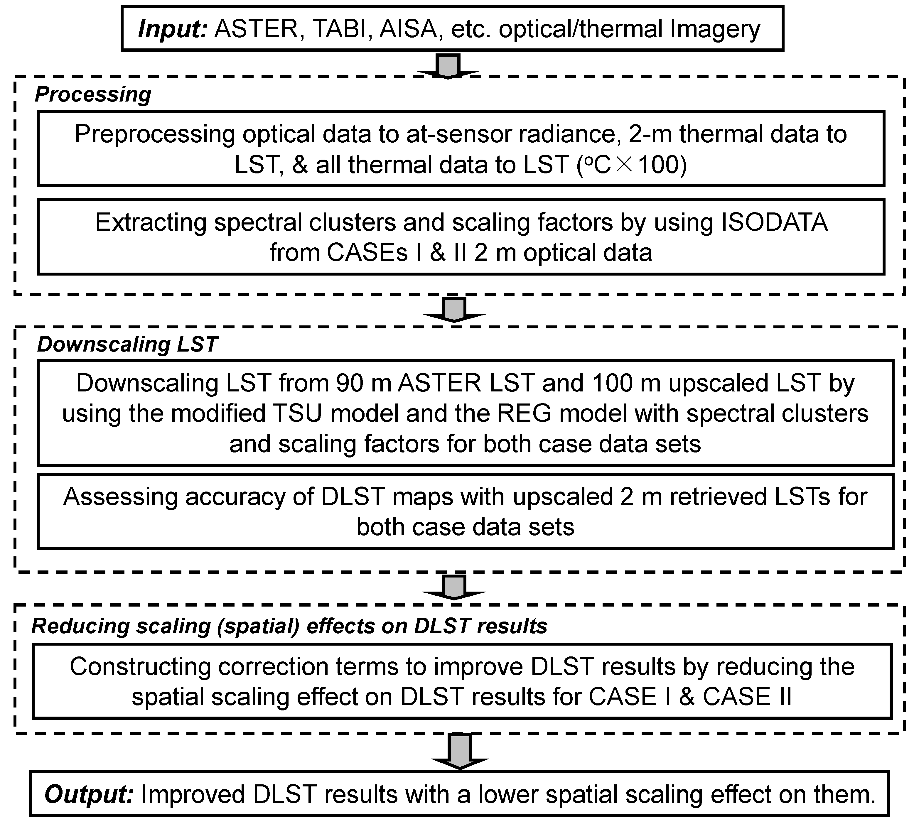
After multi-sensor thermal and optical remote sensing data were collected from the two case study areas, the proposed analysis method for reducing the scaling effect on DLST maps consists of three major components, which are summarized in Figure 2. The preprocessing component covers the following tasks: converting multispectral and hyperspectral optical data to at-sensor radiance, checking existing LST products, retrieving 2 m resolution LSTs from thermal data, converting physical units of all LST data as °C × 100, and extracting spectral clusters and scaling factors from the ten AISA VNIR bands for CASE I and the three VNIR bands for CASE II. The downscaling LST (DLST) component includes (i) downscaling the 90 m ASTER LST product for CASE I with ten spectral clusters and six scaling factors extracted from the AISA data, and (ii) downscaling the upscaled 100 m retrieved LST, aggregated from the 2 m LST data, for CASE II with ten spectral clusters and six scaling factors extracted from the three VNIR bands. A modified TSU model and a REG model were used to downscale LSTs with CASEs I and II data sets. Corresponding 90 m and 100 m resolution fraction (proportional) images of spectral clusters and scaling factors were produced. The reducing scaling effect component includes (i) computation of the combined variance (SD) of red and NIR bands at a high resolution in different moving window sizes, (ii) determination of the correction term’s expression by a semi-empirical approach, and (iii) reduction of the scaling effect on DLST maps by running the CT expression for both study areas.

3.1. Data Preprocessing

The LSTs at 2 m resolution were retrieved from the airborne TIR data acquired in both study areas [37,38,39]. Physical units of all LST data were converted into °C × 100. All airborne optical image data were converted into at-sensor radiance (W·m⁻² sr⁻¹ μm⁻¹ × 10) before extracting their spectral clusters and scaling factors at high resolutions. For CASE I data, the multi-sensor’s data acquisition date is different (see Table 1), which might result in different LST over the same land use/land cover types. To make both ASTER and TABI TIR data comparable and verifiable each other, the TABI 2 m LST was normalized to the ASTER 90 m LST by using a normalization approach introduced in [1]. To do so, the TABI 2 m LST was first aggregated to 90 m resolution (ULST) with a resampling Pixel Aggregate tool, which averaged all 2 m resolution pixel values within a 90 m resolution pixel and then exported the averaged value to the pixel, and then a pixel-based LST difference was calculated by subtracting the TABI 90 m ULST from the ASTER 90 m LST. Next, the pixel-based difference was downscaled to 2 m resolution with a bilinear interpolation resampling method [16] and, finally, each pixel value in the TABI 2 m LST image was modified by adding the downscaled 2 m LST difference to it.

3.2. Downscaling Land Surface Temperature (DLST)

3.2.1. A Modified Thermal Spectral Unmixing (TSU) Model

By referring to the basic concept of thermal spectral unmixing (TSU) model [26] for downscaling both ASTER 90 m LST (CASE I) and upscaled 100 m LST data (CASE II) to finer resolutions, we modified the TSU model to unmix a native (low) resolution LST to infer/retrieve high-resolution thermal component temperatures, using high-resolution spectral clusters as an input. Here, fractions (i.e., FL in Equation (1) below) of spectral clusters at a low resolution can be calculated through a statistical computation of all spectral clusters from all pixels at 2 m resolution within each pixel at a low resolution (e.g., there are 2025 2-m pixels each with a unique spectral cluster within a 90 m low resolution pixel). The algorithm of the modified TSU model is described as follows. Instead of using thermal radiance in the TSU model as in [26], we directly used LST at a low resolution expressed as the thermal component temperature change weighted by their fractions of spectral clusters F at a low resolution:

LST_L(1×n) = TCV_(1×m)·F_L(m×n) + ε

(1)

with min ||LST − TCV·F|| subject to F ≥ 0.

(2)

where LST_L(1×n) represents the LSTs of n low-resolution pixels (i.e., ASTER 90 m LST and upscaled 100 m LST), TCV_(1×m) is the temperatures of m thermal component components represented by m spectral clusters at a high resolution, F_L(m×n) represents the fractions of spectral clusters (thermal components) at a low resolution, and residual ε represents the variance of LST unexplained by the spectral clusters. Per Equation (1), if we know LST_L and F_L, it is easy to solve the thermal component vector via a least-square estimation (LSE) of the model [40]. In fact, in this study, we know ASTER 90 m LST and upscaled 100 m LST and the corresponding low-resolution fractions of m spectral clusters calculated from the high-resolution spectral clusters data (see Section 3.2.2). Consequently, TCV_(1×m) can be obtained via the following LSE of the model [37]:

TCV_(1×m) = LST_L(1×n)· F′_L(n×m)·(F_L(m×n)·F′_L(n×m))⁻¹

(3)

After obtaining TCV_(1×m), we can map very-high-resolution LSTs for both case data sets (2 m resolution) based on their spectral cluster maps (here, thermal components and their temperatures can be assigned to the corresponding spectral clusters) created with an ISODATA unsupervised algorithm. Then, different high-resolution LST maps can be created by aggregating the 2 m LST maps created with thermal component temperatures.

To test the power and stability of the performance of correction term (CT, introduced in Section 3.3 below), the REG model was also used to downscale the ASTER 90 m LST and the upscaled 100 m LST to different high-resolution DLSTs with corresponding 90 m (CASE I) and 100 m (CASE II) resolution six scaling factors (created by aggregating the 2 m resolution scaling factor maps). The six scaling factors include four fraction images: vegetated area, bare soil, impervious area, and water body/shadow area, and two normalized difference vegetation indices: (NIR − red)/(NIR + red) and (NIR − green)/(NIR + green). The procedure of DLST with the REG model was introduced in detail in [1].

In this study, after calculating fractions of the spectral clusters at coarse resolutions (90 m for downscaling ASTER LST and 100 m for downscaling the 100 m upscaled LST), thermal components’ temperatures at 2 m resolution were obtained by solving the modified TSU model (Equation (1)). For running the REG model, the corresponding 90 m and 100 m resolution six scaling factors were also calculated for computing the LST estimate parameters. Then, for both case studies, the 2 m high-resolution DLST maps obtained by solving the TSU model were upscaled to 6 m, 10 m, …, 62 m with a resampling Pixel Aggregation Tool. Additionally, the 2 m, 6 m, …, 62 m DLST maps were produced by using the LST estimate parameters created by running the REG model. Finally, all these DLST maps at different resolutions were modified by running a post-processing approach (see Section 3.2.4).

3.2.2. Extraction of Spectral Clusters from High Resolution Optical Data

In this study, spectral clusters, substituting for thermal components, were used to solve the modified TSU model (Equation (1)). For CASE I study area, we chose ten VNIR bands as input to the ISODATA algorithm to create three (10, 15, and 20) spectral-cluster maps to select the number of spectral clusters leading to a better LST map at a very high resolution. Likewise, the 10, 15, and 20 spectral-cluster maps were also created by the ISODATA algorithm using the three VNIR bands available for the CASE II study area.

3.2.3. Thermal Components and Spectral Clusters

Thermal components may be represented by spectral clusters because the spectral clusters can be intrinsically linked to thermal physical characteristics of thermal components (

Table 2. Mean temperature from the 2 m TABI retrieved LST, thermal component temperature, surface cover materials/types and thermal physical characteristics of spectral clusters extracted from AISA optical data by an ISODATA unsupervised algorithm.

Spectral Cluster	1 Mean T/SD from 2 m LST (°C)	2 Thermal Component T (°C)	Surface Cover Materials and Types	3 Thermal Characteristics
SC1	32.17/5.07	31.38	shaded areas, very low albedo residential areas, dark soil, water bodies	low—mid thermal radiance, more latent heat exchange
SC2	32.92/5.09	35.99	low albedo impervious areas (most residential areas and dark road surfaces)	mild—high thermal radiance, more sensible heat exchange
SC3	34.32/4.93	37.23	light gray road surface and other mild albedo impervious surfaces	high thermal radiance with sensible heat exchange
SC4	29.92/4.49	25.04	vegetated areas (turf, lawn & shrub)	low thermal radiance with latent heat exchange
SC5	34.30/4.93	35.74	mild albedo impervious areas (most parking lots, roofs)	mild—high thermal radiance, more sensible heat exchange
SC6	33.79/5.01	28.83	low albedo impervious areas (most parking lots, roofs)	mild thermal radiance, less sensible heat exchange
SC7	29.83/4.34	30.19	bright vegetated area (tree canopy)	low thermal radiance with latent heat exchange
SC8	31.51/4.47	25.90	spare vegetated areas (turf & lawn or wet bare soil)	low thermal radiance, more latent heat exchange
SC9	32.26/5.67	28.71	playground, gray bare soil.	low—mild thermal radiance, less sensible heat exchange
SC10	29.81/6.70	33.66	bright roofs	mid thermal radiance with sensible heat exchange

Note: ¹. Mean temperature / standard deviation calculated from the 2 m TABI retrieved LST for each spectral cluster. ². Thermal component temperature, created by solving the modified TSU model, for each spectral cluster. ³. Referring to [22,23,41,42].

). By referring to [22,23,41,42], the extracted spectral clusters could be associated with, and described by, corresponding surface materials and cover types that are further described by thermal physical characteristics. Table 2 lists the 10 spectral clusters resulted from CASE I data, with the corresponding surface cover materials/types and their thermal physical characteristics. Essentially, based on the above association of the extracted spectral clusters, corresponding thermal component temperatures at a high resolution are expected by solving the modified TSU model (Equation (1)).

3.2.4. Modification of Initial LSTs

In this research, the initial DLST maps were created from ASTER 90 m LST and upscaled 100 m LST by solving the modified TSU model and the REG model. To improve the initial DLSTs quality at different high resolutions, we adopted a post-processing approach suggested by [1,16] to modify the DLST maps with the residual error.

3.2.5. Validation of Downscaled LSTs

Once the DLST maps were improved by reducing the residual error, upscaled LSTs (ULSTs) from the 2 m LSTs for both study areas were used as reference to verify DLSTs at different high resolutions. ULST maps were also used to verify the DLST results corrected by the correction term, introduced below.

3.3. Correction Term (CT)

As literature reviewed in the Introduction section shows, the scaling effect in DLST processes is associated with the degree of heterogeneity of surface features/materials within pixels at specific resolutions [4,5]. Understanding this issue in different urban landscapes is especially important to study urban thermal environments, where mixed pixels are frequently dominant in moderate- (even high-) resolution remote sensing imagery [33,43]. Such a certain degree of heterogeneity within pixels at different resolutions may be denoted by the variances of red and NIR bands extracted from finer-resolution images [31,32]. In a very heterogeneous urban environment, the variances of the red and NIR radiance would be large, while their co-variance would be small [32]. By referring to the concept of the correction terms and their application in [32], in this research, we used a combined variance of red and NIR bands extracted from the high-resolution images (used as a subpixel level) to construct the CT to reduce the LST differences (i.e., the scaling effect) between the referenced (or upscaled) LSTs and the estimated DLSTs at different high resolutions. The final corrected DLST is obtained by adding the CT to the DLST (i.e., lumped model estimation in [32]).

To determine the CT expression, we first calculated the combined standard deviation (SD) of red and NIR bands from the high-resolution optical data sets of CASEs I and II by a moving window with different sizes for different resolution DLST results. Then, different difference LST (D_iffLST) maps between ULSTs and DLSTs were created at different resolutions:

D_iffLST = ULST − DLST

(4)

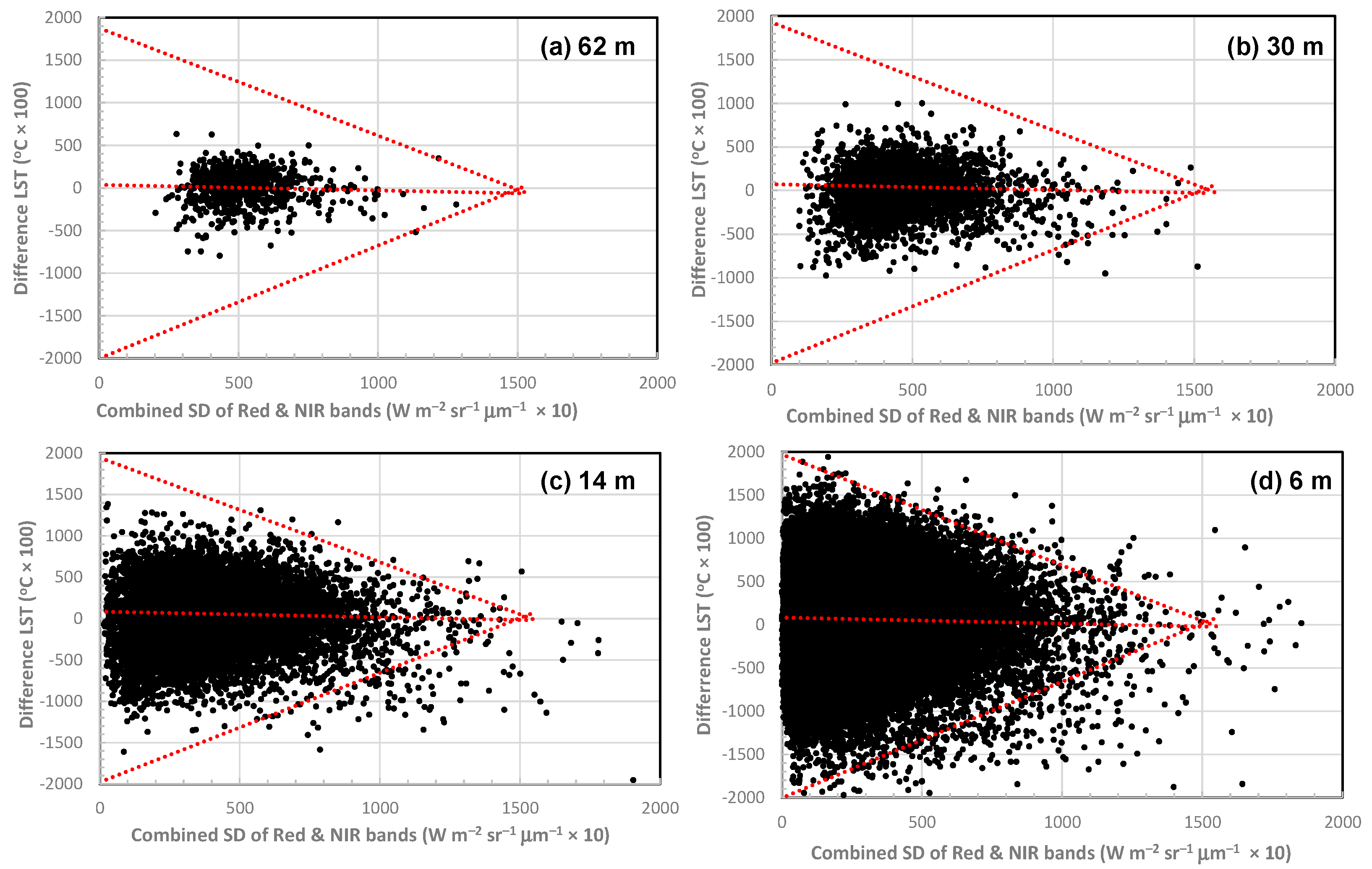
where ULST represents the upscaled LST map (i.e., the referenced LST map) from the 2 m LST, and DLST is the downscaled LST from the ASTER 90 m or the upscaled 100 m LST. Pixel values in a D_iffLST image consist of two slightly equal (symmetric) parts: negative and positive pixel value parts, which might be covered by two masks: the negative mask and the positive mask. After a careful look at the D_iffLST images, it was observed that most negative pixels are covered by low albedo surface materials and types including vegetated areas, water bodies, shadow/shaded areas, and dark/wet surfaces (e.g., roofs and road surfaces, etc.). Those negative pixels potentially have a high level of latent heat exchange, whilst most positive pixels, covered by mid-to-high albedo impervious surfaces, potentially have a high level of sensible heat exchange. Figure 3 presents the scatter plots in the feature space of D_iffLST and combined SD of red and NIR bands at 62 m, 30 m, 14 m, and 6 m resolutions, created from CASE I data. Per the scatter plots, a general pattern across the different resolutions could be observed, which is in a triangle shape with the greatest absolute value of D_iffLST toward the least combined SD of red and NIR bands, and the least absolute value (close to 0) toward the greatest combined SD value (Figure 3).

Therefore, based on the distribution of the scatter points and relationships observed between D_iffLST (Y) and the combined SD (X) of red and NIR bands, for both negative and positive parts, a linear model might be fitted as follows:

Y = A·X + B

(5)

where A and B represent the slope and intercept of the linear model. Their optimal values were determined by a semi-empirical approach via an iteration procedure. With CASE I data, the CT expression (°C × 100) was fitted as:

Y = −0.25·X + 320

(6)

which could be applied to partially reduce the scaling effect on DLST results at least for CASE I data. Specifically, for negative pixel values of D_iffLST (negative mask), the corrected DLST is obtained by subtracting the pixel-based Y values with input pixel-based X values from the corresponding pixel-based DLST map. Similarly, for positive pixel values of D_iffLST (positive mask), the corrected DLST is obtained by adding the pixel-based Y values with input pixel-based X values to the corresponding pixel-based DLST map. For CASE II data, a similar pattern of the scatter plots in the feature space of D_iffLST and combined SD of red and NIR bands at different resolutions was observed (Figure S4). Therefore, the same CT expression fitted from CASE I data might be directly used for CASE II DLSTs’ correction.

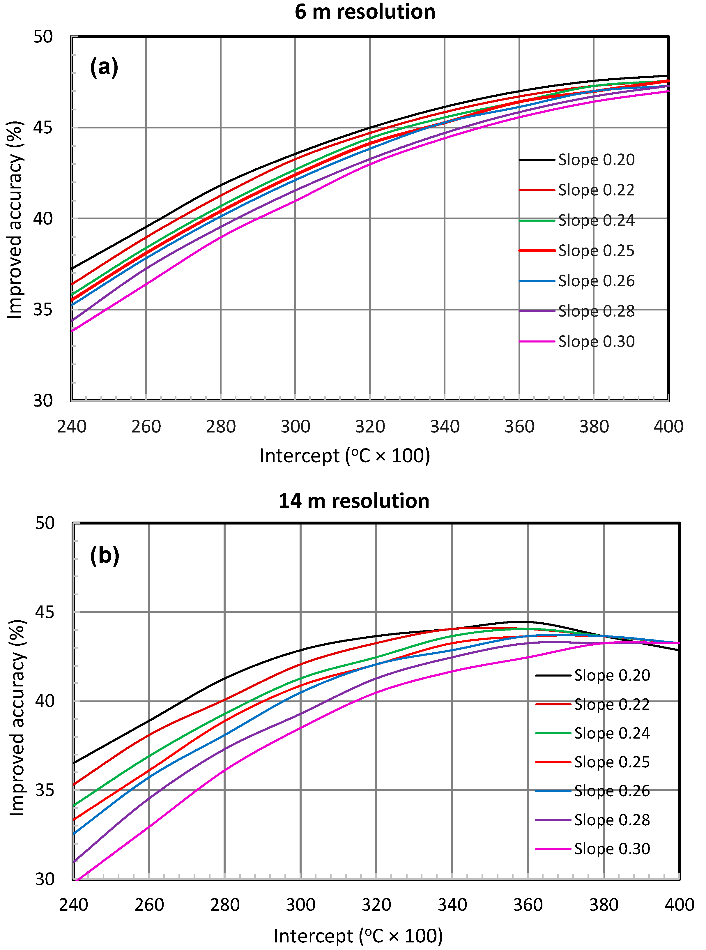
Once the CT expression (Equation (6)) was fitted, we tested its sensitivity by changing its slope value from 0.20 to 0.30 with a step = 0.02 and its intercept value from 240 to 400 with a step = 20 for CASE I DLST maps. CTs computed with different combinations of slope and intercept values were added (or subtracted) to (or from) the DLSTs at 6 m and 14 m resolutions considering the corresponding positive mask (or negative mask). Then, these corrected DLSTs at 6 m and 14 m resolutions were used to calculate the mean absolute error (MAE) (Equation (8) below) by comparing the corresponding ULST reference maps. The accuracy was obtained by calculating {(MAE without CT) − (MAE with CT)}/(MAE without CT)·100 (%). The test results were presented in Figure 4. Per the figure, the accuracy could be improved from 34% to 47% for the 6 m resolution DLST and from 30% to 44% for the 14 m resolution. This sensitive test reveals that the applications of the CT expression could result in a DLST accuracy improved at least 30%; thus, the compensation of the scaling effect in DLST processes is effective and significant. In this study, we also used the root mean square error (RMSE, Equation (7)) to indicate the power of the CT in reducing the scaling effects.

In practice, how to determine the negative and positive pixel value masks from DiffLST images is a key step to execute the CT to reduce the scaling effect on DLST results. This is because true high-resolution LST maps are not known, so the D_iffLST images are actually not available for creating both negative/positive masks for running the CT expression. In this case, we proposed a field temperature measurement approach to help create the negative and positive masks, which is introduced as follows. After obtaining the thermal component temperatures or LST estimate parameters, a high-resolution DLST (i.e., DLST at 2 m resolution for both study areas) was created. The variation of LST over the high-resolution DLST map should spatially match the spectral cluster map (i.e., each spectral cluster has a corresponding unique thermal component temperature). We can then bring the high-resolution DLST map and spectral cluster map to the field for taking in situ LST measurements with an instrument for each spectral cluster (thermal component). The in situ measurement approach could be referred to either [44] or [45]. A random sampling or systematic sampling method may be adopted to select 5–10 patches/pixels for each spectral cluster to take their in situ LST measurements. It is necessary to normalize the in situ LST measurements to the original coarse-resolution LST before creating an in situ LST map by assigning these normalized in situ measurements to the corresponding spectral clusters. Now, a D_iffLST image at a high-resolution (2 m resolution for this study) may be obtained by subtracting the DLST map from the in situ measurement LST map. Once the D_iffLST image at the high-resolution is obtained, other different resolution D_iffLST images can be created by upscaling the D_iffLST with a pixel aggregation method. In this way, the corresponding resolution masks (negative and positive) can be obtained. Since the very-high-resolution retrieved LST map is available in this study, we simply used the 2 m LST map as the in situ LST measured map to calculate a D_iffLST image at the initial 2 m resolution, then other D_iffLST images at different resolutions (i.e., 62 m, 54 m, …, 6 m) were created by aggregating the 2 m D_iffLST image.

3.4. Assessment of DLST Results

Hereafter, the “DLST” maps refer to those without correction with CT expression but modified with a post-processing approach (see Section 3.2.4), while the “corrected DLST” maps refer to those corrected with the CT expression (Equation (6)). To assess the DLST results, a comparison with the corresponding ULST maps (i.e., LST reference maps) was performed. Specifically, we compared and assessed the DLST results created without CT with those with CT correction. These evaluations were conducted in graphics (DLST maps, histograms, and scatter plots) and tabular statistics (descriptive statistics, RMSE and MAE). The RMSE and MAE were expressed as follows:

$$\mathrm{RMSE}=\sqrt{{\displaystyle \sum }_{\mathrm{i}=1}^{\mathrm{n}}{\left({\mathrm{LST}}_{\mathrm{i}}-{\widehat{\mathrm{LST}}}_{\mathrm{i}}\right)}^2/\mathrm{n}}$$

(7)

$$\mathrm{MAE}={\displaystyle \sum }_{\mathrm{i}=1}^{\mathrm{n}}\left|{\mathrm{LST}}_{\mathrm{i}}-{\widehat{\mathrm{LST}}}_{\mathrm{i}}\right|/\mathrm{n}$$

(8)

where, LST_i and ${\widehat{\mathrm{LST}}}_{\mathrm{i}}$ are the reference LST and the estimated LST corrected with or without CT correction, respectively, and n is the number of samples (pixels).

4. Results and Analysis

4.1. DLST Maps at Different High Resolutions

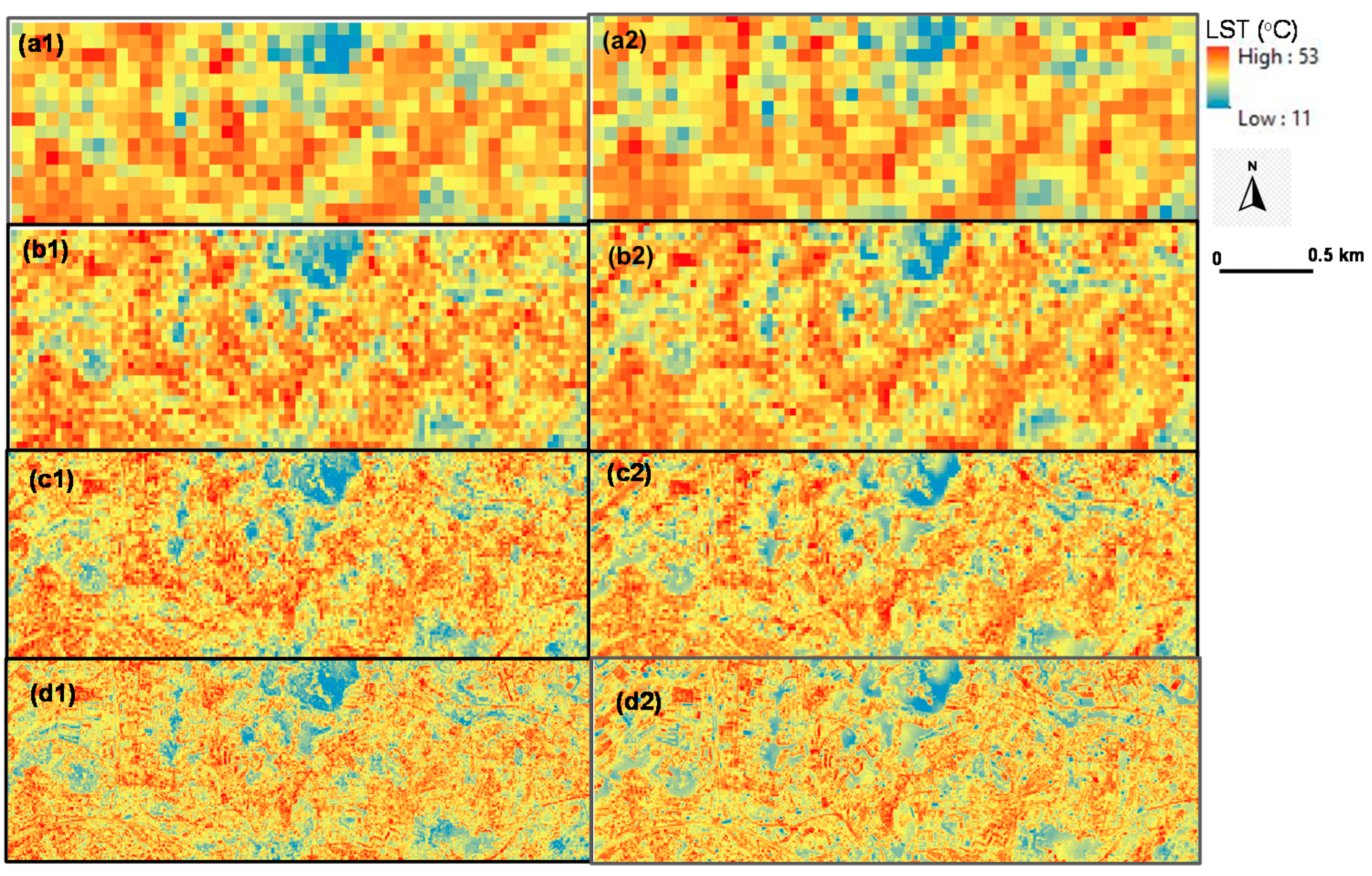
Figure 5a1–d1 presents the corrected DLST maps with CT at 62 m, 30 m, 14 m, and 6 m resolutions for CASE I; for comparison purposes, Figure 5a2–d2 shows the corresponding ULST maps (reference LSTs), aggregated from the TABI 2 m LST map. By checking and comparing the corrected DLST results and the corresponding LST references, it is clearly observed that the spatial distribution patterns and locations of LSTs were well consistent. For example, in both LST maps, the low left corner area is a relatively high-temperature zone, covered by a high density of buildings and the transportation network, whilst the upper-middle area is a low-temperature area with a large park. Figure S2 also clearly shows such patterns. Particularly, it is evident for those DLST maps at a resolution better than 30 m. The consistency of the LST spatial pattern between corrected DLST and ULST maps was also found for CASE II (maps not reported here): relatively low-temperature areas in the upper right, lower, and lower right zones due to the presence of grass, turf, and greenness; relatively high-temperature areas distributed in the left-middle zones where impervious surfaces are dominant.

Table 3. Basic descriptive statistics (°C) of DLSTs corrected with correction term (CT), downscaled from ASTER 90 m LST product and 100 m upscaled LST data by solving the modified TSU model (CASE I) with AISA 10 spectral clusters created by ISODATA and REG model (CASE II) with 6 scaling factors.

DLST (LST)	Min	Max	Mean	SD
CASE I with ASTER 90 m LST and AISA optical data (DLST by using the modified TC-based TSU model)
ASTER 90 m LST	23.05	36.95	32.65	2.04
62 m DLST	22.16	38.19	32.69	2.31
54 m DLST	23.53	37.66	32.71	2.45
46 m DLST	22.95	38.72	32.70	2.51
38 m DLST	22.22	39.24	32.68	2.65
30 m DLST	21.92	39.38	32.70	2.73
22 m DLST	21.34	40.66	32.68	2.93
14 m DLST	20.76	40.87	32.67	3.15
10 m DLST	19.31	41.83	32.64	3.33
6 m DLST	18.49	43.05	32.60	3.58
2 m DLST *	19.20	41.55	32.66	4.35
TABI 2 m retrieved LST	11.54	52.78	32.67	5.19
CASE II with high resolution thermal retrieved LST and optical data (DLST by using the REG model)
Upscaled 100 m retrieved LST	9.82	30.82	20.74	2.50
62 m DLST	12.89	31.27	20.77	2.62
54 m DLST	11.69	31.64	20.78	2.75
46 m DLST	12.99	31.47	20.78	2.79
38 m DLST	12.91	32.09	20.80	2.86
30 m DLST	11.62	32.80	20.81	3.00
22 m DLST	11.37	32.72	20.82	3.13
14 m DLST	10.42	33.65	20.82	3.36
10 m DLST	8.95	35.18	20.83	3.50
6 m DLST	5.50	35.40	20.83	3.67
2 m DLST *	1.64	34.39	20.73	3.59
2 m retrieved LST	0.00	50.00	20.75	4.88

Note: * without CT correction because the initial very high resolution optical data is 2 m (aggregating 0.5 m to 2 m for CASE II data) so that no red/NIR SD data are available at 2 m.

presents the basic descriptive statistics (Min, Max, Mean, and SD values) of the DLST results, and they are generally reasonable. Both corrected DLST maps created from CASEs I and II had a similar change tendency of the descriptive statistics across different resolutions. In addition, Table 3 also shows that the data distributions were asymmetrical: for CASE I, the data distributions were biased to the right side (maximum), while for CASE II, they were slightly biased to the left side (minimum). Both unsymmetrical phenomena can be illustrated by Figure 1: the CASE I study area presents more impervious surfaces/built up areas than greenness and water body areas, while the CASE II study area shows slightly more greenness and rural areas than impervious surfaces/built up areas.

4.2. Accuracy of DLST Maps

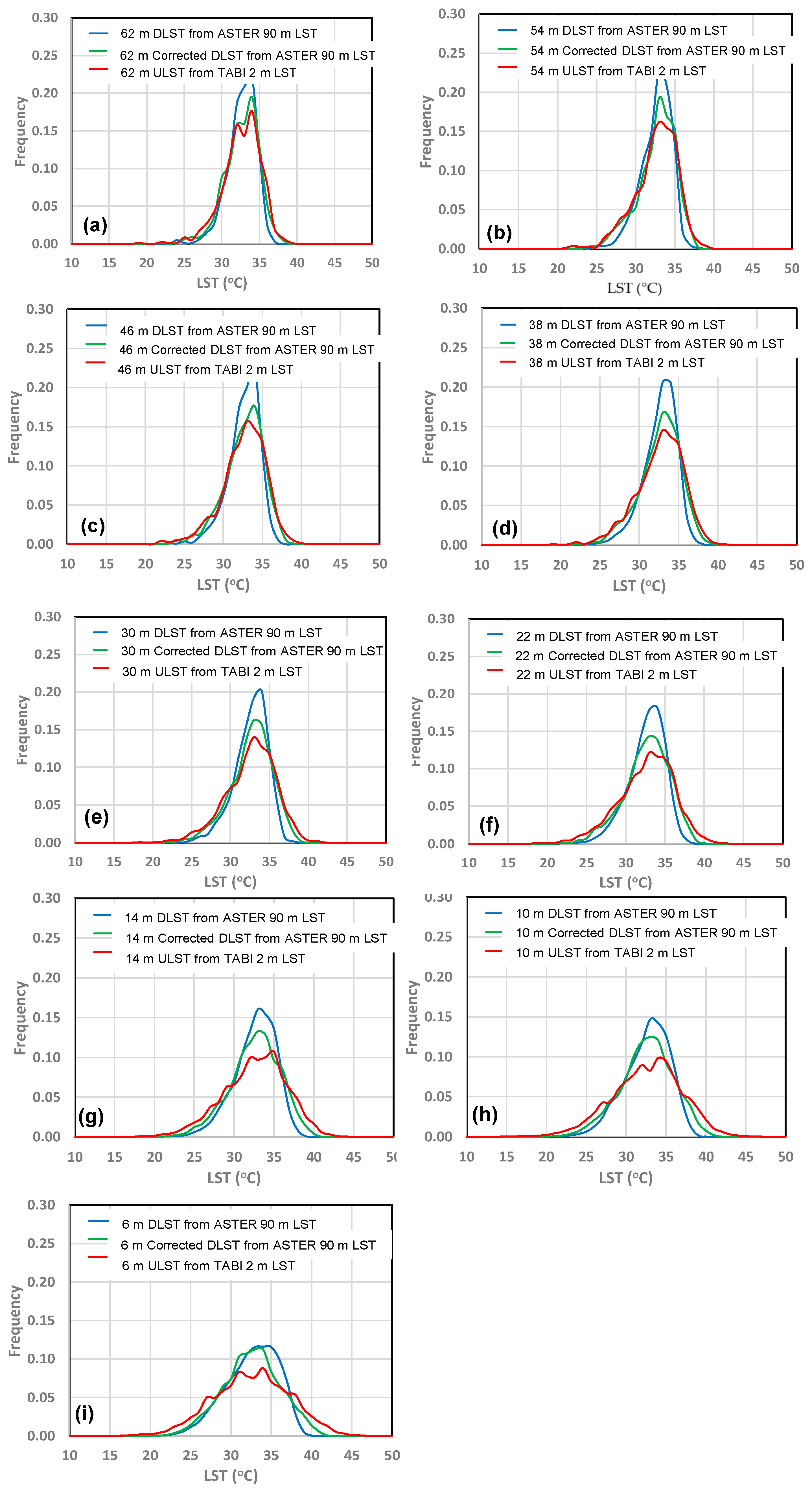
Figure 6 shows the histograms of three types of LST maps (at 62 m, 54 m, …, 6 m resolutions) created with CASE I data: the DLST maps, the corrected DLST maps, and the corresponding LST reference maps (ULST). By checking the LST changes across different resolutions and comparing shapes and proximity of the two DLST map histograms to the ULST map histogram in the same plots, we could easily observe the following three points. (1) The histogram curves of both DLST and corrected DLST maps at lower resolutions (lower than 30 m) were closer to the corresponding LST reference maps, suggesting that the scaling effect on the DLST maps is less than those at finer resolutions (better than 30 m). (2) With the improvement of the resolutions (from 62 m to 2 m), the minimum and maximum pixel values for the three LST maps (shown along the X-axis) decrease and increase, respectively (also see Table 3), indicating that the proportion of pure pixels, covered by individual surface materials/cover types (thermal components), increases. (3) The histogram curves of the corrected DLST maps were closer to the corresponding LST reference maps, especially at resolutions better than 30 m. This means that the CT significantly reduced the scaling effect on DLST maps, especially for the very-high resolutions.

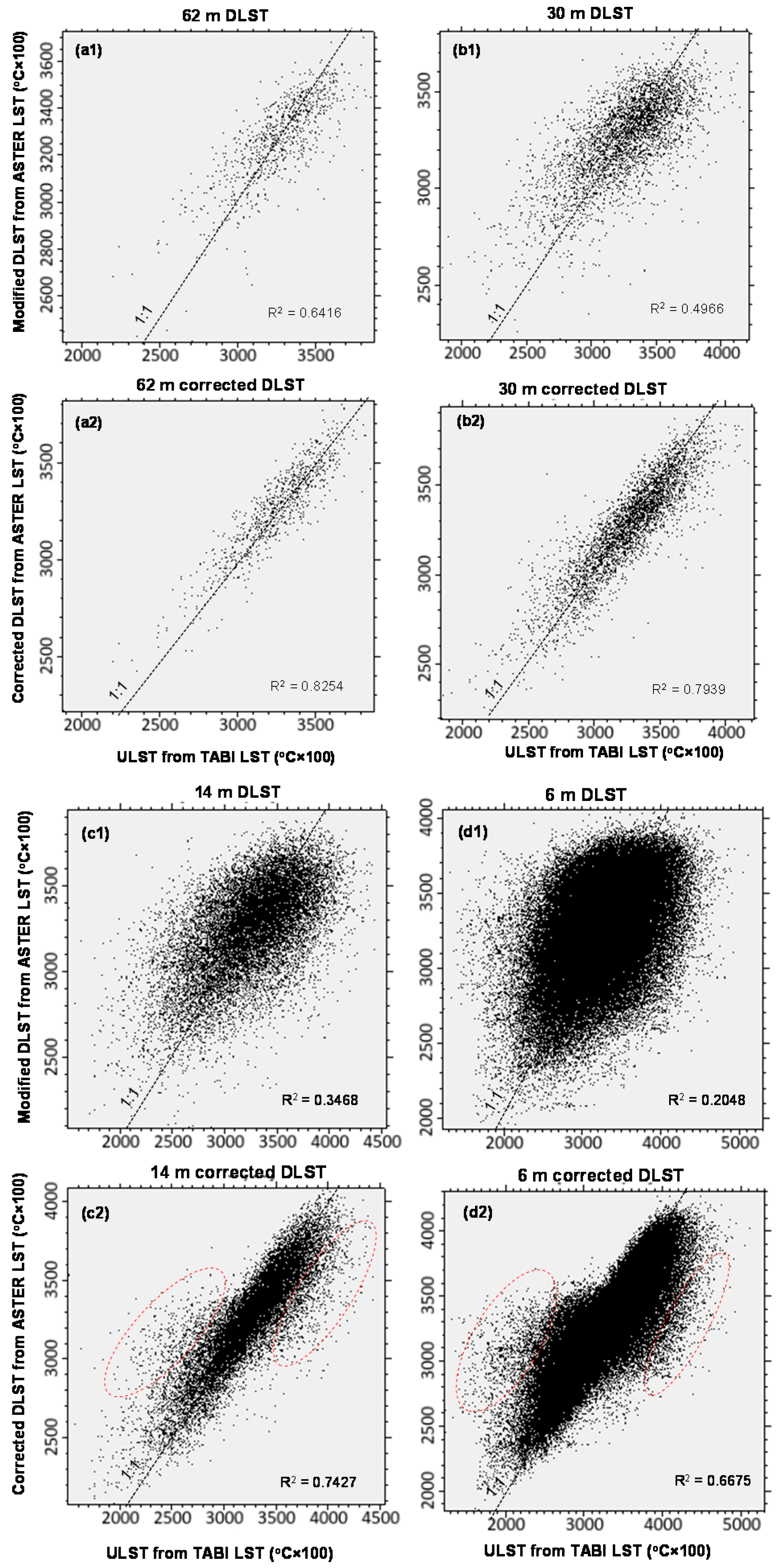
Scatter plots in Figure 7 present the correlations (R²) and consistencies between the DLST maps with and without CT and the corresponding LST reference maps. Per the scatter plots, besides the first two points we observed from Figure 6 (i.e., less scaling effect on DLST maps at lower resolutions and smaller minimum and greater maximum values for the DLST maps at higher resolutions), compared to the plots of Figure 7a1–d1, the scatter points in Figure 7a2–d2 were closer to the 1:1 scale line, demonstrating that the corrected DLST maps had a more proximate distribution to, and spatial patterns as, the thermal information shown in the corresponding ULST maps. By comparing the R² values of DLST and corrected DLSTs for corresponding resolutions, the increase in R² after correction with CT was significant (R² value for corrected DLSTs increased of 0.18 for 62 m to 0.46 for 6 m with respect to the DLST maps). The results suggested that using CT to reduce the scaling effect on DLST maps is workable and effective. The same scatter plots at different resolutions for CASE II also demonstrate the effectiveness of using CT to improve DLST maps (Figure S5).

Table 4. Summary of RMSE and MAE values improved with correction term (CT) to correct DLSTs for CASEs I and II data sets. All bold numbers mean “Average”.

DLST	RMSE (°C)			MAE(°C)			Note
	W/out CT	With CT	Improved with CT (%)	W/out CT	With CT	Improved with CT (%)
CASE I with ASTER 90 m LST and AISA optical data (DLST by using the TC-based TSU model)
62 m DLST	1.55	1.07	30.97	1.17	0.85	27.35	compared to ULST of TABI 2m LST
54 m DLST	1.67	1.14	31.74	1.28	0.89	30.47	compared to ULST of TABI 2m LST
46 m DLST	1.85	1.22	34.05	1.41	0.94	33.33	compared to ULST of TABI 2m LST
38 m DLST	2.04	1.32	35.29	1.57	1.00	36.31	compared to ULST of TABI 2m LST
30 m DLST	2.30	1.48	35.65	1.77	1.11	37.29	compared to ULST of TABI 2m LST
22 m DLST	2.67	1.69	36.70	2.05	1.23	40.00	compared to ULST of TABI 2m LST
14 m DLST	3.24	2.05	36.73	2.52	1.46	42.06	compared to ULST of TABI 2m LST
10 m DLST	3.69	2.33	36.86	2.90	1.64	43.45	compared to ULST of TABI 2m LST
6 m DLST	4.4	2.78	36.82	3.49	1.95	44.13	compared to ULST of TABI 2m LST
Average			34.98			37.15
CASE II with high resolution thermal retrieved LST and optical data (DLST by using the REG model)
62 m DLST	1.97	1.33	32.49	1.32	0.84	36.36	compared to ULST of retrieved 2m LST
54 m DLST	2.02	1.33	34.16	1.34	0.81	39.55	compared to ULST of retrieved 2m LST
46 m DLST	2.16	1.42	34.26	1.45	0.86	40.69	compared to ULST of retrieved 2m LST
38 m DLST	2.36	1.57	33.47	1.58	0.92	41.77	compared to ULST of retrieved 2m LST
30 m DLST	2.50	1.61	35.60	1.67	0.95	43.11	compared to ULST of retrieved 2m LST
22 m DLST	2.77	1.86	32.85	1.84	1.06	42.39	compared to ULST of retrieved 2m LST
14 m DLST	3.13	2.11	32.59	2.09	1.19	43.06	compared to ULST of retrieved 2m LST
10 m DLST	3.39	2.29	32.45	2.28	1.30	42.98	compared to ULST of retrieved 2m LST
6 m DLST	3.73	2.52	32.44	2.52	1.43	43.25	compared to ULST of retrieved 2m LST
Average			33.37			41.46

summarizes the RMSE and MAE values for DLST (W/out CT in the table) and corrected DLST maps, as well as the accuracy improvement after DLST maps were corrected with the same CT expression (Equation (6)), for CASEs I and II. Per the table, it is apparent that after correction, the RMSE and MAE values were significantly reduced at different resolutions (i.e., the accuracy was significantly increased). The average RMSE value across 6 m to 62 m resolutions was reduced by 35% and the average MAE value by 37% in the CASE I study area. For CASE II data, when considering the DLST maps estimated with the REG model (Table 4) or the modified TSU model (Table S1), the average RMSE value across 6 m to 62 m resolutions was reduced by 33% (or 30% in Table S1) and the average MAE value by 41% (or 33% in Table S1).

5. Discussion

5.1. The Performance of the Modified TSU Model

In this research, the modified TSU model was effective in downscaling LSTs from a coarse resolution to different high resolutions (before considering the correction with CT expression). Unlike using thermal radiance in the thermal component unmixing-based techniques in [26], directly using LST at a low resolution in the TSU model (expressed as thermal component temperature change weighted by spectral cluster fractions) is less time consuming, and it is easy to obtain different high-resolution DLST maps. For both case data sets, we tested and compared three different numbers (10, 15, and 20) of spectral clusters used for solving the modified TSU model, and the DLST results were similar, but the 10 spectral clusters consumed less time for the model solving. The modified TSU model with the CASE I data led to slightly better DLST results (relatively lower RMSE and MAE values) compared with our previous results [1] created by artificial neural networks and REG with AISA data derived scaling factors, especially for very-high resolutions. The accurate and reliable DLST maps produced with the modified TSU model were also better than, or comparable to, those in existing literature (e.g., [12,46,47]). However, the scaling effect on the DLST maps at high resolutions (better than 30 m) was still significant.

Directly using multiple spectral clusters created with high-resolution optical data and ISODATA algorithm to solve the modified TSU model for obtaining thermal component temperatures was proved to be workable. The multiple spectral clusters might be used to represent thermal components to unmix the model. For this case, it may be expected that the modified TSU model with extracted spectral clusters from optical data can also be used for downscaling a coarse-resolution LST (e.g., AVHRR and MODIS data) to a moderate resolution LST (e.g., similar to Landsat and ASTER data), although we did not test it in this study. In fact, the different spectral clusters could be described by different surface materials and cover types (see Table 2), and different thermal components may consist of different hot and cold components. The hot components represent objects that have a relatively high thermal radiance, such as impervious areas (roofs and roads), and the cold components are objects that have a relatively low thermal radiance, such as vegetated areas and water bodies [42]. Research results indicate there exist associations of LSTs with different urban biophysical descriptors (impervious surface, vegetation, and soil) and with thermal feature fractions (hot and cold components) [42]. Deng and Wu [23] selected five categories of land cover types to explain the thermal responses of urban land cover types. Therefore, the thermal components may be denoted by spectral clusters and surface materials/cover types, such as impervious surfaces, vegetated areas, water bodies, etc., which may be relatively easy to be extracted and mapped by using traditional classification methods and optical data. However, from Table 2, although the thermal component temperatures among the 10 spectral clusters were mostly different (here, one thermal component has only one temperature), the mean temperatures/SDs calculated from the 2 m TABI LST for the 10 spectral clusters were obviously overlaid if their distributions (SDs) were considered. This implies that although the spectral clusters representing thermal components are workable, they are not perfect in solving the modified TSU model.

5.2. Corection Term (CT)

In this study, to develop an appropriate correction term (an association of correcting DLST with input SD of red and NIR bands), we tested a linear regression model, non-linear polynomial forms (second and third order), and artificial neural network models, and found that the corrected DLST results were all not ideal (i.e., reducing D_iffLST not significant). Therefore, we adopted a semi-empirical approach (a linear model) and determined its slope and intercept through running an iteration procedure by changing slope and intercept values. We finally found that the CT expression of Equation (6) was effective in reducing the spatial scaling effect on DLSTs created by using both models (the modified TSU model and the REG model) with both case data sets.

The sensitive tests for CASE I (Figure 4) with different combinations of slope and intercept indicated that the CT expression, Equation (6), was stable. The CT application could result in at least 30% increased accuracy for the high-resolution DLSTs. Thus, the CT expression (Equation (6)) was effective and significant. By checking the testing results, the effectiveness of the CT expression was enhanced with the refinement of the resolution of the DLST maps (Table 4), which was just matching the increase in the scaling effect in DLST processes with the increase in the resolution of the DLST maps. The effectiveness of the CT expression was dependent on the two masks (negative and positive) of the D_iffLST images and on the point distribution patterns in the feature space (D_iffLST image and the combined SD of red and NIR bands). After checking the point patterns in the feature space of DLST maps created with artificial neural networks and REG models [1] for CASE I data, we found similar patterns to those shown in Figure 3 across different spatial resolutions. Such similar distribution patterns (i.e., a triangle shape) were also observed for CASE II data with both the REG model (Figure S4) and the modified TSU model. Therefore, Equations (5) and (6) are expected to be generally workable.

Given the fact that the D_iffLST images at different higher resolutions are not available in practice, as pointed out in Section 3.3, how to determine the negative and positive masks from D_iffLST images is a critical issue. Per an application perspective of downscaling coarse LST data to finer resolutions, a field in situ LST measurement approach may be a solution. For instance, one of the approaches proposed and used by [44,45] may be suggested. A random sampling or systematic sampling may be adopted to select 5–10 patches/pixels for each spectral cluster (thermal component or surface cover type) to take their in situ LST measurements. Sampled pixels/patches are required > 3 × 3 pixels (6 × 6 m² at a 2 m resolution) in which the thermal component/surface cover material/type is homogenous to ensure that the in situ LST measurement from its central pixel fully represents the thermal component/surface cover material/type and avoids any boundary effects from different surfaces. The in situ LST measuring time is required to be as close as possible to the data acquired by the remote sensing sensors (e.g., within ± one hour). In addition, it is necessary to normalize the in situ LST measurements to the original coarse-resolution LST before creating an in situ LST map. Once such an in situ LST map is created, different-resolution D_iffLST images can be produced by upscaling the original resolution D_iffLST (2 m in this study) with a pixel aggregation resampling method. Strictly following the requirement of taking the in situ LST measurements in the field as discussed above, the quality of the D_iffLST map can be ensured such that both negative and positive masks are reliably created for running the CT expression. Since the two masks are created based on the negative and positive relative values (not on the absolute values of D_iffLST map), even though the in situ LST measurements may not be very accurate (e.g., ±1 °C error), the effect on both masks’ quality is small and thus might be ignored. Therefore, the field-temperature-measuring approach may not significantly influence the feasibility of the proposed method.

5.3. Limitations and Significance of This Study

The current CT expression could be used to partially reduce the scaling effect (improved accuracy > 30%). However, there still exists an observable part of error (the scaling effect), which needs to be considered to further correct. This error is present in the DLST maps at very high resolutions, and it is mostly associated with those scattered points within the red dash ellipses in Figure 7(c2,d2), Figure S3(d2,e2) and Figure S5(c2,d2). There may be two directions to further correct the scaling effect on DLST maps at very high resolutions: (1) also considering the co-variance of red and NIR bands in the CT expression, not just the combined variance (SD), especially for a relative homogenous research area/environment [32]; (2) considering the CT expression in a non-linear form focusing on a heavier correction of the scaling effect corresponding to the lower values of the combined SD and/or co-variance of red and NIR bands.

Overall, the results of improving DLST maps with the proposed method were stable and significant. Although the two study areas were relatively small compared to a big city area, they cover typical land surface materials and types reflecting corresponding thermal physical characteristics in heterogenous urban environments. In addition, many applications in different areas need high-resolution thermal data, including LST maps created by using different advanced downscaling methods. For example, studies on urban heat island and landscapes may need very-high-resolution LST products (e.g., to 2–4 m) [13,16,48]. Therefore, the results and derived conclusions in this study with the proposed method are significant and novel in reducing the scaling effect on DLST results and can make a substantial contribution to the relevant literature. The method, coupled with the modified TSU model, should also be useful in other urban environments.

6. Conclusions

In this research, the main aim is to propose and test a new method to reduce scaling effect on DLST maps at different high resolutions. To do so, considering two case study data sets, we first applied a modified TSU model and an REG model to directly downscale the LSTs at coarse resolutions to DLSTs at finer resolutions. Then, after the modification of the DLST maps for their residual error, a new method with the CT expression, Equation (6), was used to reduce the scaling effect. The experimental results indicate that the proposed method was effective and significant, especially reducing the scaling effect on DLST maps at very high resolutions. Therefore, the novel significance for the proposed method is directly reducing this scaling effect at finer resolutions. Specifically, the following three conclusions could be derived from the result analysis:

• The modified TSU model for unmixing thermal component temperatures at the initial high resolution was effective and advanced in downscaling LSTs compared to our previous works and those in existing literature.
• Spectral clusters were intrinsically associated with spectral properties of surface materials/cover types and thermal physical characteristics of corresponding thermal components, and were thus workable and reliable for solving the modified TSU model.
• The proposed method with the CT expression (Equation (6)) was workable and the testing results were reliable and stable for the two data sets; thus, it is effective and novel.

The proposed method was tested for the first time in this study and could be expected to improve DLST results created by any advanced downscaling LST methods. However, how to determine the negative and positive masks from D_iffLST images at higher resolutions is a key issue for efficiently using the CT technique. A field in situ LST measurement approach is recommended for creating the initial D_iffLST image (other higher-resolution D_iffLST images can be derived by upscaling the initial D_iffLST image). How to further reduce the scaling effect on DLST maps at very high resolutions: the co-variance of red and NIR bands, especially for relatively homogeneous areas, and the CT expression in a non-linear form may be considered in the future research.

References

- Pu, R. Assessing scaling effect in downscaling land surface temperature in a heterogenous urban environment. Int. J. Appl. Earth Obs. Geoinf. 2021, 96, 102256. [Google Scholar] [CrossRef]
- Zhou, J.; Liu, S.; Li, M.; Zhan, W.; Xu, Z.; Xu, T. Quantification of the scale effect in downscaling remotely sensed land surface temperature. Remote Sens. 2016, 8, 975. [Google Scholar] [CrossRef] [Green Version]
- Wu, H.; Li, W. Downscaling land surface temperatures using a random forest regression model with multitype predictor variables. IEEE Access 2019, 7, 21904–21916. [Google Scholar] [CrossRef]
- Garrigues, S.; Allard, D.; Baret, F.; Weiss, M. Quantifying spatial heterogeneity at the landscape scale using variogram models. Remote Sens. Environ. 2006, 103, 81–96. [Google Scholar] [CrossRef]
- Garrigues, S.; Allard, D.; Baret, F. Influence of the spatial heterogeneity on the nonlinear estimation of Leaf Area Index from moderate resolution remote sensing data. Remote Sens. Environ. 2006, 106, 286–298. [Google Scholar] [CrossRef]
- Kustas, W.P.; Norman, J.M.; Anderson, M.C.; French, A.N. Estimating subpixel surface temperatures and energy fluxes from the vegetation index–radiometric temperature relationship. Remote Sens. Environ. 2003, 85, 429–440. [Google Scholar] [CrossRef]
- Agam, N.; Kustas, W.P.; Anderson, M.C.; Li, F.; Neale, C.M.U. A vegetation index based technique for spatial sharpening of thermal imagery. Remote Sens. Environ. 2007, 107, 545–558. [Google Scholar] [CrossRef]
- Chen, X.H.; Yamaguchi, Y.; Chen, J.; Shi, Y.S. Scale effect of vegetation-index-based spatial sharpening for thermal imagery: A simulation study by ASTER data. IEEE Geosci. Remote Sens. Lett. 2012, 9, 549–553. [Google Scholar] [CrossRef]
- Ghosh, A.; Joshi, P.K. Hyperspectral imagery for disaggregation of land surface temperature with selected regression algorithms over different land use land cover scenes. ISPRS J. Photogramm. Remote Sens. 2014, 96, 76–93. [Google Scholar] [CrossRef]
- Liu, H.; Weng, Q. Scaling effect of fused ASTER-MODIS land surface temperature in an urban environment. Sensors 2018, 18, 4058. [Google Scholar] [CrossRef]
- Gao, F.; Kustas, W.P.; Anderson, M.C. A data mining approach for sharpening thermal satellite imagery over land. Remote Sens. 2012, 4, 3287–3319. [Google Scholar] [CrossRef] [Green Version]
- Mukherjee, S.; Joshi, P.; Garg, R. A comparison of different regression models for downscaling Landsat and MODIS land surface temperature images over heterogeneous landscape. Adv. Space Res. 2014, 54, 655–669. [Google Scholar] [CrossRef]
- Bonafoni, S.; Tosi, G. Downscaling of land surface temperature using airborne high-resolution data: A case study on Aprilia, Italy. IEEE Geosci. Remote Sens. Lett. 2017, 14, 107–111. [Google Scholar] [CrossRef]
- Gao, L.; Zhan, W.; Huang, F.; Quan, J.; Lu, X.; Wang, F.; Ju, W.; Zhou, J. Localization or globalization? Determination of the optimal regression window for disaggregation of land surface temperature. IEEE Trans. Geosci. Remote Sens. 2017, 55, 477–490. [Google Scholar] [CrossRef]
- Li, X.; Xin, X.; Jiao, J.; Peng, Z.; Zhang, H.; Shao, S.; Liu, Q. Estimating subpixel surface heat fluxes through applying temperature-sharpening methods to MODIS data. Remote Sens. 2017, 9, 836. [Google Scholar] [CrossRef] [Green Version]
- Zawadzka, J.; Corstanje, R.; Harris, J.; Truckell, I. Downscaling Landsat-8 land surface temperature maps in diverse urban landscapes using multivariate adaptive regression splines and very high resolution auxiliary data. Int. J. Digit. Earth 2020, 13, 899–914. [Google Scholar] [CrossRef] [Green Version]
- Yang, G.; Pu, R.; Zhao, C.; Huang, W.; Wang, J. Estimation of subpixel land surface temperature using an endmember index based technique: A case examination on ASTER and MODIS temperature products over a heterogeneous area. Remote Sens. Environ. 2011, 115, 1202–1219. [Google Scholar] [CrossRef]
- Hutengs, C.; Vohland, M. Downscaling land surface temperatures at regional scales with random forest regression. Remote Sens. Environ. 2016, 178, 127–141. [Google Scholar] [CrossRef]
- Xia, H.; Chen, Y.; Li, Y.; Quan, J. Combining kernel-driven and fusion-based methods to generate daily high spatial resolution land surface temperatures. Remote Sens. Environ. 2019, 224, 259–274. [Google Scholar] [CrossRef]
- Xu, S.; Zhao, Q.; Yin, K.; He, G.; Zhang, Z.; Wang, G.; Wen, M.; Zhang, N. Spatial downscaling of land surface temperature based on a multi-factor geographically weighted machine learning model. Remote Sens. 2021, 13, 1186. [Google Scholar] [CrossRef]
- Li, W.; Ni, L.; Li, Z.-L.; Duan, S.-B.; Wu, H. Evaluation of machine learning algorithms in spatial downscaling of MODIS land surface temperature. IEEE J. Sel. Top. Appl. Earth Obs. Remote Sens. 2019, 12, 2299–2307. [Google Scholar] [CrossRef]
- Deng, C.; Wu, C. Examining the impacts of urban biophysical compositions on surface urban heat island: A spectral unmixing and thermal mixing approach. Remote Sens. Environ. 2013, 131, 262–274. [Google Scholar] [CrossRef]
- Deng, C.; Wu, C. Estimating very high resolution urban surface temperature using a spectral unmixing and thermal mixing approach. Int. J. Appl. Earth Obs. Geoinf. 2013, 23, 155–164. [Google Scholar] [CrossRef]
- Ma, J.; Zhang, W.; Marinoni, A.; Gao, L.; Zhang, B. An improved spatial and temporal reflectance unmixing model to synthesize time series of Landsat-like images. Remote Sens. 2016, 10, 1388. [Google Scholar] [CrossRef] [Green Version]
- Zhu, X.; Cai, F.; Tian, J.; Williams, T. Spatiotemporal fusion of multisource remote sensing data: Literature survey, taxonomy, principles, applications, and future directions. Remote Sens. 2018, 10, 527. [Google Scholar] [CrossRef] [Green Version]
- Wang, J.; Schmitz, O.; Lu, M.; Karssenberg, D. Thermal unmixing based downscaling for fine resolution diurnal land surface temperature analysis. ISPRS J. Photogramm. Remote Sens. 2020, 161, 76–89. [Google Scholar] [CrossRef]
- Zhan, W.; Chen, Y.; Zhou, J.; Wang, J.; Liu, W.; Voogt, J.; Zhu, X.; Quan, J.; Li, J. Disaggregation of remotely sensed land surface temperature: Literature survey, taxonomy, issues, and caveats. Remote Sens. Environ. 2013, 131, 119–139. [Google Scholar] [CrossRef]
- Jin, Y.; Yong, G.; Wang, J.; Chen, Y.; Heuvelink, G.B.M.; Peter, M.; Atkinson, P.M. Downscaling AMSR-2 Soil Moisture Data with Geographically Weighted Area-to-Area Regression Kriging. Trans. Geosci. Remote Sens. 2018, 56, 2362–2376. [Google Scholar] [CrossRef] [Green Version]
- Zhao, W.; Wen, F.; Wang, Q.; Sanchez, N.; Piles, M. Seamless downscaling of the ESA CCI soil moisture data at the daily scale with MODIS land products. J. Hydrol. 2021, 603, 126930. [Google Scholar] [CrossRef]
- Garrigues, S.; Allard, D.; Baret, F.; Morisette, J. Multivariate quantification of landscape spatial heterogeneity using variogram models. Remote Sens. Environ. 2008, 112, 216–230. [Google Scholar] [CrossRef]
- Hu, Z.; Islam, S. A framework for analyzing and designing scale invariant remote sensing algorithms. IEEE Trans. Geosci. Remote Sens. 1997, 35, 747–755. [Google Scholar]
- Hu, Z.; Islam, S. Effects of subgrid-scale heterogeneity of soil wetness and temperature on grid-scale evaporation and its parameterization. Int. J. Climatol. 1998, 18, 49–63. [Google Scholar] [CrossRef]
- Liu, H.; Weng, Q. Scaling effect on the relationship between landscape pattern and land surface temperature: A case study of Indianapolis, United States. Photogramm. Eng. Remote Sens. 2009, 75, 291–304. [Google Scholar] [CrossRef] [Green Version]
- Wikipedia, City of Yokohama, Japan. Available online: https://en.wikipedia.org/wiki/Yokohama#Climate (accessed on 23 May 2021).
- World Weather Online, Aprilia Weather, Lazio, IT. Available online: https://www.worldweatheronline.com/aprilia-weather/lazio/it.aspx (accessed on 23 May 2021).
- Yamaguchi, Y.; Kahle, A.B.; Tsu, H.; Kawakami, T.; Pniel, M. Overview of advanced spaceborne thermal emission and reflection radiometer (ASTER). IEEE Trans. Geosci. Remote Sens. 1998, 36, 1062–1071. [Google Scholar] [CrossRef] [Green Version]
- Qin, Z.; Karnieli, A.; Berliner, P. A mono-window algorithm for retrieving land surface temperature from Landsat TM data and its application to the Israel-Egypt border region. Int. J. Remote Sens. 2001, 22, 3719–3746. [Google Scholar] [CrossRef]
- Sobrino, J.A.; Jimenez-Munoz, J.C.; Paolini, L. Land surface temperature retrieval from LANDSAT5 TM. Remote Sens. Environ. 2004, 90, 434–440. [Google Scholar] [CrossRef]
- Pu, R.; Gong, P.; Michishita, R.; Sasagawa, T. Assessment of multi-resolution and multi-sensor data for urban surface temperature retrieval. Remote Sens. Environ. 2006, 104, 211–225. [Google Scholar] [CrossRef]
- Pu, R.; Xu, B.; Gong, P. Oakwood crown closure estimation by unmixing of Landsat TM data. Int. J. Remote Sens. 2003, 24, 4433–4445. [Google Scholar] [CrossRef]
- Wilson, J.S.; Clay, M.; Martin, E.; Stuckey, D.; Vedder-Risch, K. Evaluating environmental influences of zoning in urban ecosystems with remote sensing. Remote Sens. Environ. 2003, 86, 303–321. [Google Scholar] [CrossRef]
- Lu, D.; Weng, Q. Spectral mixture analysis of ASTER images for examining the relationship between urban thermal features and biophysical descriptors in Indianapolis, Indiana, USA. Remote Sens. Environ. 2006, 104, 157–167. [Google Scholar] [CrossRef]
- Weng, Q.; Fu, P.; Gao, F. Generating daily land surface temperature at Landsat resolution by fusing Landsat and MODIS data. Remote Sens. Environ. 2014, 145, 55–67. [Google Scholar] [CrossRef]
- Coll, C.; Caselles, V.; Galve, M.; Valor, E.; Niclòs, R.; Sánchez, J.M.; Rivas, R. Ground measurements for the validation of land surface temperatures derived from AATSR and MODIS data. Remote Sens. Environ. 2005, 97, 288–300. [Google Scholar] [CrossRef]
- White-Newsome, J.L.; Brines, S.J.; Brown, D.G.; Dvonch, J.T.; Gronlund, C.J.; Zhang, K.; Oswald, E.M.; O’Neill, M.S. Validating satellite-derived land surface temperature with in situ measurements: A public health perspective. Environ. Health Perspect. 2013, 12, 925–931. [Google Scholar] [CrossRef] [PubMed] [Green Version]
- Jeganathan, C.; Hamm, N.A.S.; Mukherjee, S.; Atkinson, P.M.; Raju, P.L.N.; Dadhwal, V.K. Evaluating a thermal image sharpening model over a mixed agricultural landscape in India. Int. J. Appl. Earth Obs. Geoinf. 2011, 13, 178–191. [Google Scholar] [CrossRef]
- Bisquert, M.; Sánchez, J.M.; Caselles, V. Evaluation of disaggregation methods for downscaling MODIS land surface temperature to Landsat spatial resolution in Barrax test site. IEEE J. Sel. Top. Appl. Earth Obs. Remote Sens. 2016, 9, 1430–1438. [Google Scholar] [CrossRef]
- Sobrino, J.A.; Oltra-Carrió, R.; Sòria, G.; Bianchi, R.; Paganini, M. Impact of spatial resolution and satellite overpass time on evaluation of the surface urban heat island effects. Remote Sens. Environ. 2012, 117, 50–56. [Google Scholar] [CrossRef]
Figure 1.
Location maps of the two case study areas (CASE I study area, Yokohama City, Japan; and CASE II study area, Aprilia City, Italy) where thermal/optical data were collected. The study areas are displayed with standard false color composite images (NIR/red/green vs. R/G/B).
Figure 2.
Flowchart showing the main processing components of downscaling LST and reducing scaling effect on DLSTs from ASTER 90 LST and upscaled 100 m retrieved LST, with spectral clusters and scaling factors extracted from the high-resolution optical data.
Figure 3.
Scatter plots in a two-dimension feature space of the difference (DiffLST) between ULSTs and DLSTs (created by the modified TSU model) and the combined SD of red and NIR bands. Plots (a–d) were created with 62 m, 30 m, 14 m, and 6 m resolution map data with CASE I data set. The remaining 54 m, 46 m, 38 m, 22 m, and 10 m plots (Figure S1, see all figures and tables with S * in Supplementary Materials section) have a similar triangle-shape pattern as Figure 3.
Figure 4.
Sensitivity tests of the correction term (Y = slope · X + intercept) by changing its slope and intercept values for CASE I. The improved accuracy of the DLST with CT compared with the DLST without CT is reported for 6 m (a) and 14 m (b) resolutions.
Figure 5.
Corrected DLST maps downscaled from ASTER 90 m LST with AISA data-derived spectral clusters, by applying the modified TSU model. (a1–d1) are 62 m, 30 m, 14 m, and 6 m DLST maps, and (a2–d2) are the corresponding ULST maps (reference LSTs) upscaled from the TABI 2 m LST map. The remaining 54 m, 46 m, 38 m, 22 m, and 10 m LST maps are reported in Figure S2.
Figure 6.
Histograms of 62 m, 54 m, 46 m, 38 m, 30 m, 22 m, 14 m, 10 m, and 6 m DLST maps without CT (in dashed line, (a–i)) and with CT (corrected DLST, in dotted line, (a–i)), downscaled from ASTER 90 m LST with AISA data (CASE I, using the modified TSU model), and histograms of the corresponding ULSTs (in solid line, (a–i)) aggregated from the TABI 2 m LST.
Figure 7.
Scatter plots (CASE I) between DLST results (a1–d1) and corrected DLST results (a2–d2) with the CT expression (Equation (6)), and corresponding ULST aggregated from the TABI 2 m LST. The DLST results were created from ASTER 90 m LST with AISA data derived 10 spectral clusters and by using the modified TSU model. The remaining 54 m, 46 m, 38 m, 22 m, and 10 m LST scatter plots (Figure S3) had the similar differences between DLST and corrected DLSTs as Figure 7.