
SafeNet: SwArm for Earthquake Perturbations Identification Using Deep Learning Networks


1
Institute of Earthquake Forecasting, China Earthquake Administration, Beijing 100036, China
2
College of Instrumentation and Electrical Engineering, Jilin University, Changchun 130061, China
3
Istituto Nazionale di Geofisica e Vulcanologia, Via di Vigna Murata 605, 00143 Rome, Italy
4
National Institute of Natural Hazards, Ministry of Emergency Management of China, Beijing 100085, China
*
Author to whom correspondence should be addressed.
Remote Sens. 2021, 13(24), 5033; https://doi.org/10.3390/rs13245033
Submission received: 2 November 2021
/
Revised: 8 December 2021
/
Accepted: 8 December 2021
/
Published: 10 December 2021
(This article belongs to the Special Issue Ionosphere Monitoring with Remote Sensing)
Abstract
:Low Earth orbit satellites collect and study information on changes in the ionosphere, which contributes to the identification of earthquake precursors. Swarm, the European Space Agency three-satellite mission, has been launched to monitor the Earth geomagnetic field, and has successfully shown that in some cases it is able to observe many several ionospheric perturbations that occurred as a result of large earthquake activity. This paper proposes the SafeNet deep learning framework for detecting pre-earthquake ionospheric perturbations. We trained the proposed model using 9017 recent (2014–2020) independent earthquakes of magnitude 4.8 or greater, as well as the corresponding 7-year plasma and magnetic field data from the Swarm A satellite, and excellent performance has been achieved. In addition, the influence of different model inputs and spatial window sizes, earthquake magnitudes, and daytime or nighttime was explored. The results showed that for electromagnetic pre-earthquake data collected within a circular region of the epicenter and with a Dobrovolsky-defined radius and input window size of 70 consecutive data points, nighttime data provided the highest performance in discriminating pre-earthquake perturbations, yielding an F1 score of 0.846 and a Matthews correlation coefficient of 0.717. Moreover, SafeNet performed well in identifying pre-seismic ionospheric anomalies with increasing earthquake magnitude and unbalanced datasets. Hypotheses on the physical causes of earthquake-induced ionospheric perturbations are also provided. Our results suggest that the performance of pre-earthquake ionospheric perturbation identification can be significantly improved by utilizing SafeNet, which is capable of detecting precursor effects within electromagnetic satellite data.
1. Introduction
The ionosphere is an important layer of the solar-terrestrial space observation environment, and the process of earthquake preparation and occurrence can also cause anomalous changes in ionospheric parameters over the preparation zone, known as seismic ionospheric disturbances. These phenomena are a manifestation of earthquakes in the ionosphere, a result of lithosphere–atmosphere–ionosphere coupling, and are considered to be one of the more promising ideas for detecting short-term earthquake signals. Decades ago, Moore [1] and Davies and Baker [2] first reported anomalous ionospheric perturbations associated with the 1964 Alaska earthquake in the USA, and studies on seismic ionospheric phenomena have been rapidly developed. With the accumulation of available observational resources, seismic ionospheric phenomena have been detected, reported, and confirmed [3]. Currently, these phenomena are an issue of great concern and have become a hot topic at the intersection of seismology and space physics. In the 21st century, with the development of space satellite observation technology, many countries launched satellites dedicated to monitoring space environment changes and natural disaster activities such as earthquakes and volcanoes, for example the QuakeSat (USA), SICH-1M (Ukraine), COMPASS-2 (Russia), DEMETER (France), and China Seismo Electromagnetic Satellite (CSES). Furthermore, even satellites dedicated to other scientific purposes have been demonstrated to provide important observations for seismic ionospheric disturbances, such as the Swarm constellation of the European Space Agency (ESA). The Swarm constellation consists of three identical satellites that carry the same payloads. The combined observation of multiple satellites in the Swarm constellation offers significant advantages over single-satellite observations, allowing for better detection efficiency, better global coverage in a day, higher spatial resolution, and improved capabilities for analyzing anomalies. In this way, Swarm represents a new, successful approach to the study of seismic ionospheric phenomena.
Studies of these phenomena from the Swarm satellites are currently ongoing, yielding continuous investigation and reporting of the valuable description of their mechanisms. A review of previous studies on seismic ionospheric phenomena based on Swarm satellites shows that the work is generally divided into two types: earthquake case studies and statistical investigations, both of which focus on the analysis of ionospheric disturbance phenomena associated with the preparation phase of an earthquake before its occurrence. Both types explore the precursor and provide related criteria potentially useful for earthquake prediction and forecasting.
Various perturbations have been observed using Swarm data before the occurrence of large earthquakes. De Santis et al. [4] investigated magnetic field anomalies from Swarm data for one month before and after the magnitude 7.8 Nepal earthquake that occurred on 25 April 2015 at 06:26 UTC, and found that the cumulative number of anomalies followed the same typical power-law behavior of a critical system close to its critical time, thereafter returning to normal after the earthquake. In another study, Marchetti et al. [5] used multi-parameters from ground and space, that is, Earth geomagnetic field data (magnetic data from the ESA Swarm constellation and from L’Aquila and Duronia ground observatories of the INGV (Italian National Institute of Geophysics and Vulcanology)) along with the MERRA-2 climatological dataset to study the lithosphere–atmosphere–ionosphere coupling effects of the 2016–2017 central Italy earthquake sequence. They revealed anomalies in the ground-based geomagnetic observations 275 and 85 days before the earthquake sequence, anomalies from satellite observations 240 days and 3 days before the start of the earthquake sequence, and two perturbations in the chemical/physical composition of the atmosphere 200 and 150 days prior to the earthquake sequence. In a further study, Marchetti et al. [6] analyzed the Swarm satellite magnetic data prior to the magnitude 7.1 California Ridgecrest earthquake that occurred on 6 July 2019 and found some increase in anomalies in the Y (eastern) component of the magnetic field around 200 days before the earthquake; moreover, 15 min before the earthquake, the Swarm Bravo satellite passed right over the epicentral region, and its Y component presented interesting anomalies. Zhu et al. [7] analyzed ionospheric magnetic field data from the Swarm Alpha satellite before the 16 April 2016 Ecuador earthquake (magnitude 7.8) based on the non-negative matrix factorization method and found that the energy and entropy of one of the weighting components were more concentrated within the preparation region of the seismic event. In that study, the cumulative number of orbits with anomalies inside that region showed an acceleration before the Ecuador earthquake and recovered to a linear (i.e., standard) trend after the earthquake. In addition to the aforementioned examples, numerous studies have confirmed that the Swarm ionospheric perturbations are sensitive enough and useful for detecting earthquake-related anomalies, such as for the 2014 Ludian earthquake [8], 2017 Sarpol-e Zahab (Iran) earthquake [9], 2017 Mexico earthquake [10], and the above mentioned 2016 Ecuador earthquake [11,12].
Statistical analysis is a common technique for investigating ionospheric anomalies that occur before earthquakes using satellite data [13,14,15]. De Santis et al. [16] statistically analyzed the Swarm electron density and magnetic field data observed by the three Swarm satellites over 4.7 years using a superposed epoch approach and found that some electron density and magnetic anomalies were significantly concentrated from more than two months before the earthquake to a few days prior to the earthquake. This confirmed the well-known Rikitake empirical law between the time of the precursors and the magnitude of the earthquake by studying different magnitude ranges. In another statistical analysis of 5.3 years of magnetic field data from the Swarm satellite by Marchetti et al. [17], the distance from the satellite to the earthquake epicenter matched the measured distance arrival time of the coseismic disturbance from the surface to the ionosphere, confirming that observed anomalies were likely to be caused by seismic events due to their occurrence with a mixed transmission mechanism, i.e., by acoustic gravity waves and electromagnetic propagation in the ionosphere.
However, most existing pre-earthquake anomaly studies are lacking in consistent analysis methods and anomaly evaluation metrics; thus, the analysis results of anomalies lack universality and often lead to various or even contradictory interpretations for the same earthquake. Moreover, statistical studies of seismic anomalies often do not consider the influence of non-seismic anomalies.
Deep learning, which has been widely used in recent earthquake research [18,19,20,21,22], could perform consistent analysis and assessment of a large number of earthquakes, and could take into account the influence of non-seismic anomalies, which are an effective tool to solve the above issue. By investigating different DEMETER satellite datasets, Xiong et al. [21] confirmed some frequency bands with low-frequency electric and magnetic fields to be the main features for pre-seismic electromagnetic perturbation identification using deep learning. Xiong et al. [23] also proposed a deep learning framework termed SeqNetQuake by training whole life cycle dataset from the DEMETER satellites and transferring the well-trained model to the CSES satellite to form a new identification model which achieved a 12% improvement in classification performance. Based on the classical AdaBoost machine learning algorithm and the feature of satellite remote sensing products such as infrared and hyperspectral gases, Xiong et al. [22] proposed a novel earthquake prediction framework based on inverse boosting pruning trees (IBPT), and achieved promising forecasting results in the validation of global earthquake cases retrospectively.
In this study, we use deep learning techniques, combined with multi-year accumulated Swarm satellite data for pre-seismic ionospheric disturbance identification. The proposed method, known as SafeNet (SwArm for Earthquake study using deep learning networks), is a deep-learning method based on a sequence-based classification neural network for pre-earthquake perturbation identification. The suggested model was trained using 9017 recent independent 4.8+ magnitude earthquakes and 7-year plasma and magnetic field data from the Swarm A satellite. The results indicated that nighttime data provided the best performance in distinguishing pre-earthquake perturbations, with an F1 score of 0.846 and a Matthews correlation coefficient of 0.717. It also worked effectively in detecting pre-seismic ionospheric abnormalities as earthquake magnitude increased. Furthermore, the findings of this study enabled us to propose a hypothesis regarding the physical mechanism behind earthquake-induced ionospheric disturbances. In general, SafeNet could considerably enhance the effectiveness of pre-earthquake ionospheric perturbation identification.
This paper is organized as follows. In Section 2, the used data from the Swarm satellite and its data pre-processing are discussed, together with the observation cases of the anomalies before two actual earthquakes. Section 3 describes the network structure design and performance evaluation metrics for the proposed deep learning model. The results are analyzed and discussed in Section 4, and a hypothesis of the earthquake mechanism is presented. In Section 5, we provide a conclusion and further possible orientation for future work.
2. Datasets and Observations
2.1. The Swarm Satellites
The Swarm constellation is the first ESA constellation program for geomagnetic observation, whose main scientific objective is to study the delicate structure of the Earth’s magnetic field, its dynamics, and its interaction with Earth systems [24,25]. The constellation consists of three identically equipped satellites, Swarm A (Alpha), B (Bravo), and C (Charlie), which were launched together into a near-polar orbit on 22 November 2013, and finalized their commissioning on 17 April 2014. For the main purpose of the Swarm constellation, each satellite is equipped with a high-precision magnetometer in addition to several other sensors to increment the scientific satellites’ capabilities. Among them, the charged particle sensor (Langmuir detector) provides a new avenue for the study of the seismic ionosphere phenomena.
2.2. Earthquake Case Study
2.2.1. 2016 Sumatra Earthquake
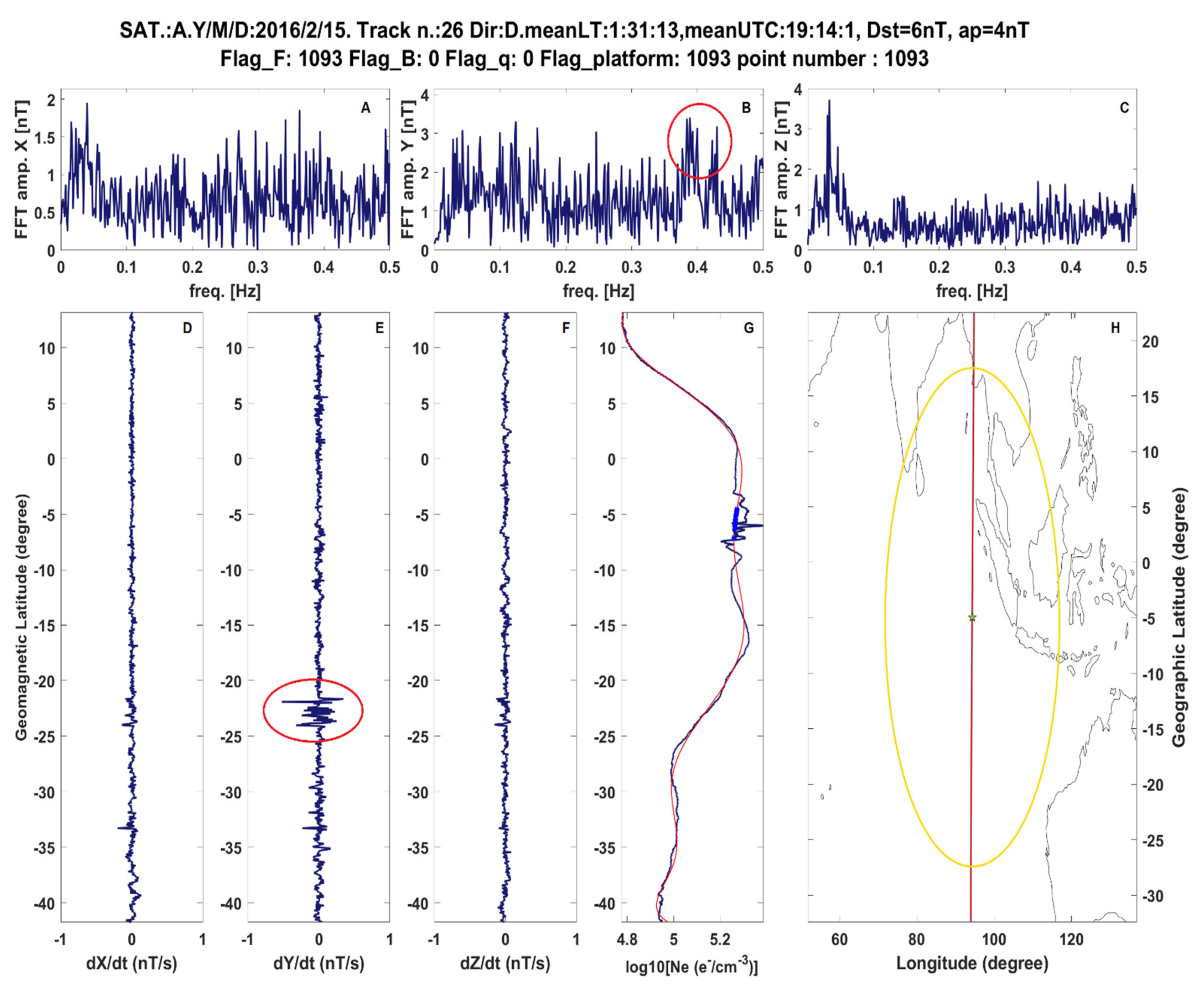
Figure 1 shows the Earth magnetic field and electron density residuals as obtained by applying the MASS (MAgnetic Swarm anomaly detection by Spline analysis) method (De Santis et al. [4]) to the data measured by the Swarm Alpha satellite on 15 February 2016, i.e., 16 days before the Mw = 7.8 Sumatra 2016 earthquake localized at 4.952°S, 94.330°E, and 24 km depth. The magnetic track shows a clear anomaly highlighted by a red circle in panel E only in the Y-East component; this is compatible for signals coming from below (i.e., the internal ones, Pinheiro et al. [26]). The FFT (fast Fourier transform) spectrum shows a signature highlighted by a red circle in panel B at about 0.4 Hz (i.e., a period of 2.5 s) that could correspond to the frequency of the anomaly. Such a signature is not visible in the track without evident anomalies (the amplitude at this frequency is normally lower than the level in this figure as visible in the other examples in Text S1, Supplementary Materials). The electron density shows the clear EIA diurnal profile, but it is quite unusual that it appeared during nighttime (local time of about 1:30 a.m.). Furthermore, the electron density shows some disturbances at +5° geographic latitude and even they do not coincide with the magnetic anomaly; both phenomena could be produced by the preparation phase of this large earthquake. Geomagnetic indices Dst = 6 nT and ap = 4 nT depict a very quiet geomagnetic condition. Thus, all the investigated measurements show an unusual status of the ionosphere in the nighttime of 15 February 2016, without known external perturbations; furthermore, the longitude of the satellite matched with the one of the future epicenters, so finally we can consider this track a good candidate for an earthquake precursor.
A complete investigation of nighttime Swarm Alpha from this track until earthquake occurrence is presented in Text S1 of the Supplementary Materials. Some days are affected by perturbed geomagnetic conditions and thus do not permit searching for possible seismo-induced ionospheric disturbances. Instead, on at least other 3 days (21, 25, and 26 February 2016), there are interesting signals: all of them present higher signal content in the Y-East component with respect to the vertical and North ones. These anomalies, detected inside Dobrovolsky’s area and a few days before earthquake occurrence, can in principle be good candidates for precursors.
2.2.2. The Ecuador Earthquake Occurred on 16 April 2016
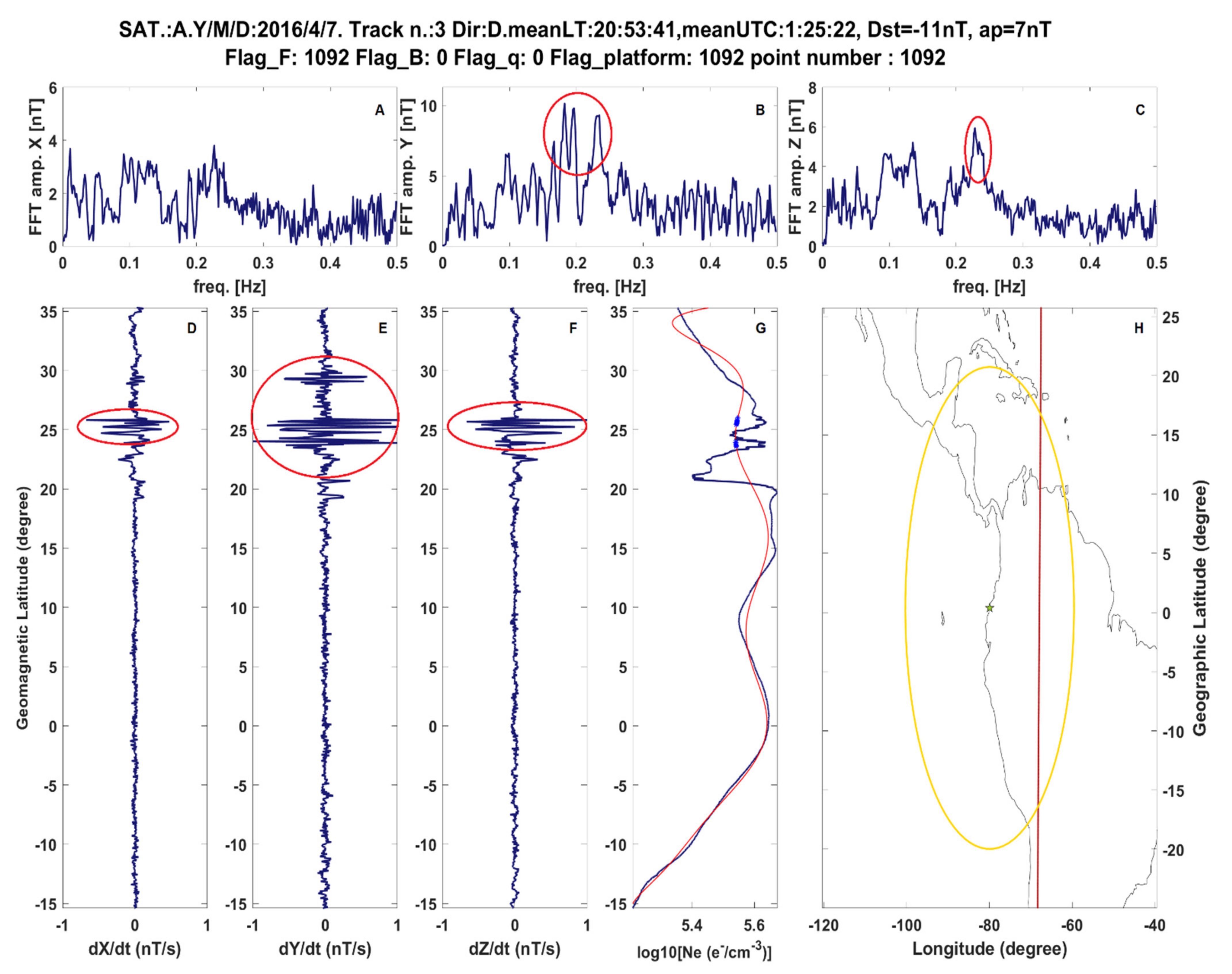
A similar example to the previous one was recorded before the Ecuador earthquake occurred on 16 April 2016 at 0.371° N, 79.940° W, and 20.6 km depth by the Swarm Alpha satellite on 19 January 2019 (see Figure 2). Akhoondzadeh et al. [12] found a pattern, in terms of the chain of phenomena, in the lithosphere–atmosphere and ionosphere in preparation of the Ecuador earthquake. In particular, they detected an increase of Swarm magnetic anomalies about 9 days before the event and during geomagnetic quiet conditions; these were probably related to the preparation phase of this seismic event. The track shown in Figure 2 is one example acquired during such an increase of anomalies and it shows an anomaly in three components of the magnetic field highlighted by red circles in panels D, E, and F. We notice that in the Y-East component the anomaly seems to have a longer duration with respect to the other components and a northern anomalous signal (even if this second North disturbance is formally out of the Dobrovolsky area). From the frequency point of view, in this case the highest intensity in the Y-East FFT spectrum (see panel B) seems to be located around 0.2 Hz (period of 5 s) with some frequency spread, and in particular it seems that there is a double peak at lower frequencies (0.182 Hz and 0.197 Hz) not present in Z FFT (see panel C), while the peak at 0.23 Hz is present also in the Z component as highlighted by the red circle in panel C. Future investigations are necessary to check by a systematic approach if a particular frequency is more prone to identifying possible seismo-induced phenomena. From the multiparametric and multi-instruments investigation, it is possible to note that there is a depletion of electron density which mostly coincides in latitude with the magnetic disturbance. A common alteration of the magnetic field with a decrease of electron density is probably a sign of the crossing of a “plasma bubble”. This feature, which is produced for the standard behavior of the ionosphere, can be also induced by air ionization in the preparation of an earthquake [27]. The earthquake was recently re-investigated by another method by Zhu et al. [7], confirming the previous result and offering new insights.
Also, for the case study in Text S2 (Supplementary Materials), from the Swarm Alpha nighttime data, one track for each day was shown until the earthquake’s occurrence. In this case, most of the other detected anomalies were probably associated with external geomagnetic activity.
2.3. Dataset and Preprocessing
All three satellites in the Swarm constellation carry the same scientific payloads to detect ionospheric electromagnetic parameters. This study focused on the use of magnetic field and plasma parameter data from the Swarm A satellite and space weather data. The types of sensors and data utilized in the study are described as follows:
(1) The vector magnetometer (VFM) is a fluxgate magnetometer from which the on-ground processor provides both high-frequency (50 Hz) and low-frequency (1 Hz) signals. The magnetic field intensity is available in an instrumental reference system as well as in the Earth one (which is used in this study), consisting of three components, X (North), Y (East), and Z (Vertical), and is measured in nT, while time is measured in Universal Time. The VFM measures field components with an accuracy of 0.1 nT every 3 months for signals at global scales within a space resolution of 20 km [25]. In this study, we focus on the X, Y, and Z components of the low-frequency (1 Hz) data.
(2) The Langmuir probe (LP) measures the electron temperature (Te), electron density (Ne), and other parameters of plasma by measuring the current generated by electrons and ions at a sampling rate of 1 Hz. This study used plasma Ne data from a level 1b product [24,25].
(3) To avoid effects caused by space weather events, we collected the Kp index, an indicator of global geomagnetic activity, to be used as an auxiliary means of discriminating between solar (or geomagnetic activity) and seismic ionospheric disturbance phenomena. It should be noted that data corresponding to periods with a Kp index greater than 3.0 were not analyzed in this study.
The data used for this study were from Swarm A and included the parameters mentioned above, collected from 1 April 2014 to 30 April 2020, i.e., 7 years of data. According to the United States Geological Survey, 18,621 earthquakes with magnitudes greater than or equal to 4.8 were reported during this period. Thus, we used the same technique as reported by Yan et al. [14] to exclude aftershocks from the list of earthquakes in order to prevent mixing pre- and post-seismic effects. After this process, the final list comprised 9017 independent earthquakes. We also removed data that corresponded to the aftershocks.
To test the reliability of the machine learning methods and improve their robustness, we created the same number of artificial non-seismic events as actual earthquakes, while randomizing and changing the timings and locations to avoid overlapping with real earthquakes. Within the selected spatio-temporal range, we sampled latitude, longitude, and time at random, adhering to the following constraints: (1) the latitude or longitude is not within 10° of the latitude or longitude of a real earthquake and (2) the time is not within 15 days of the occurrence time of a real earthquake.
3. Methodology
Figure S25 (Supplementary Materials) depicts a flowchart diagram of the methodology used in this study. To begin, a total of 9017 earthquakes with magnitudes of 4.8 or higher were extracted from seismic catalogues considering those that occurred all over the world for the study. Thirteen datasets were built by combining different magnitudes of earthquakes and features. Each dataset was divided into two parts: training data and test data. After that, we used the “sliding window” technique for data preprocessing, and lastly, we generated time series-based features.
In our work, we explored the effect of different model input and spatial window sizes, earthquake magnitudes, and whether the earthquake occurred during the day or at night using different datasets. We also performed a comparison of five state-of-the-art approaches. Considering these approaches are highly sensitive to parameter selection, we preferred to choose those configurations that would allow us to achieve the highest performance in the tests. The performance of each approach was then evaluated after the parameter selection. Finally, we evaluated the performance of each technique using ROC curves and other performance metrics.
3.1. Data Preprocessing
A variety of reasons, including satellite payload interference, the space environment, and other factors, may produce inaccuracies in constantly observed satellite data. As a precaution against such mistakes, we divided continuous observation data into fixed-length sliding windows (commonly known as “sequences”), which we then utilized as inputs to our proposed model. We also divided the data into sliding windows that were continuous but did not overlap because time series data are highly autocorrelated sequences. As a result, we carefully examined the difference between the first and final data points ordered by time in each time window to verify that the data were continuous. Time series windows with unreasonable time differences (i.e., gaps) were removed from the analysis.
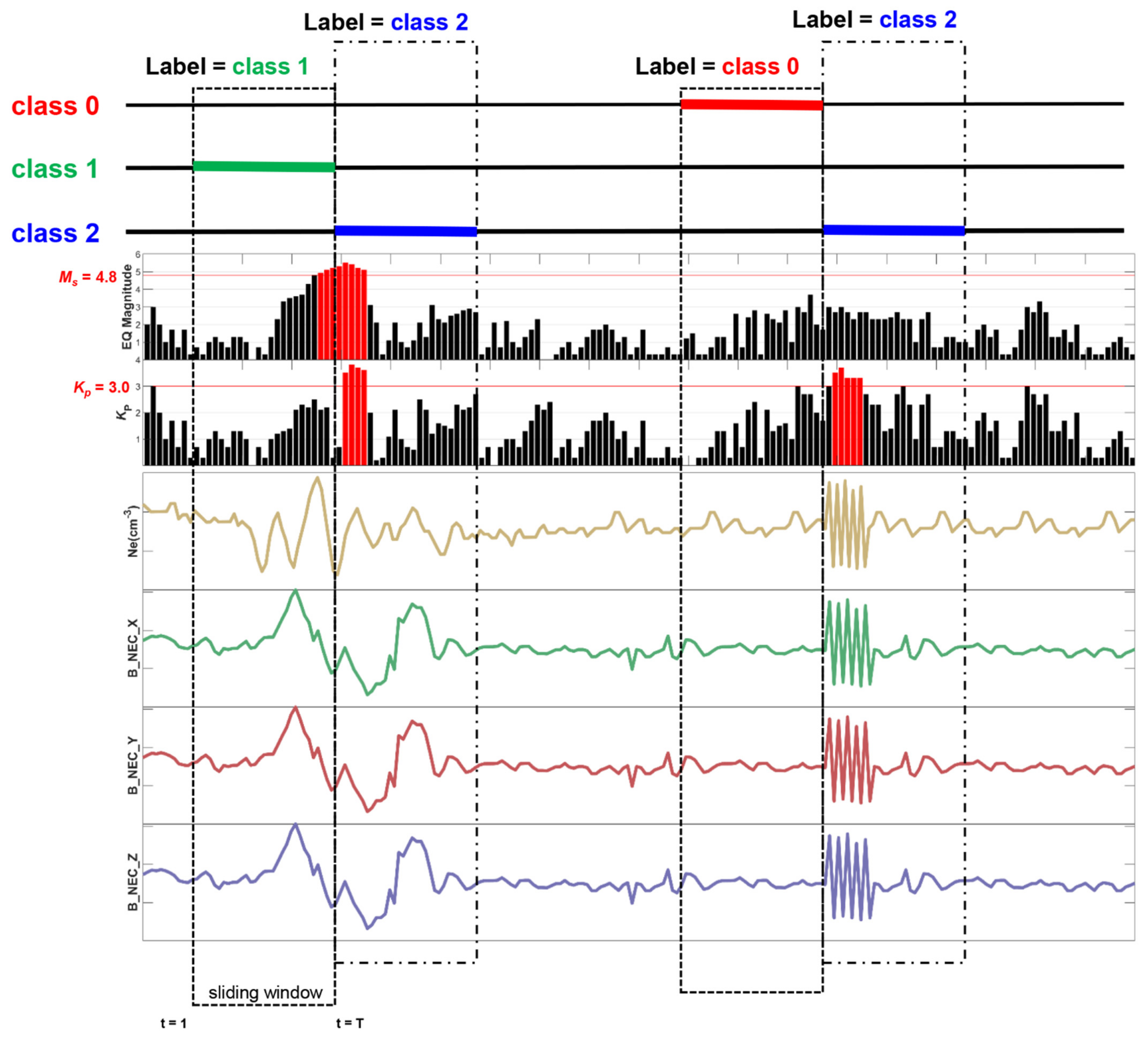
Subsequently, we reformulated the pre-earthquake ionospheric perturbation discrimination task as a multiclass multivariate time-series classification problem with the data marked as follows (Figure 3): the non-seismic-related data were marked as 0, seismic-related data were marked as 1, and data with a Kp index greater than 3.0, regardless of whether the data were related to an earthquake, were marked as 2, indicating density perturbations due to solar and magnetic activity [30]. It is known that the Earth’s magnetic field undergoes temporal fluctuations and exhibits recognized patterns related to the movement of the poles, and time series data exhibit significant autocorrelation characteristics, which indicates that the field is highly variable. Therefore, to ensure that the overall Swarm dataset could be utilized effectively, it was carefully divided into two contiguous parts: the first 80 percent (in chronological order) of the data was used for model training (the training set), and the last 20 percent was used for model testing and final assessment (the test set).
3.2. Deep Learning Network Architecture
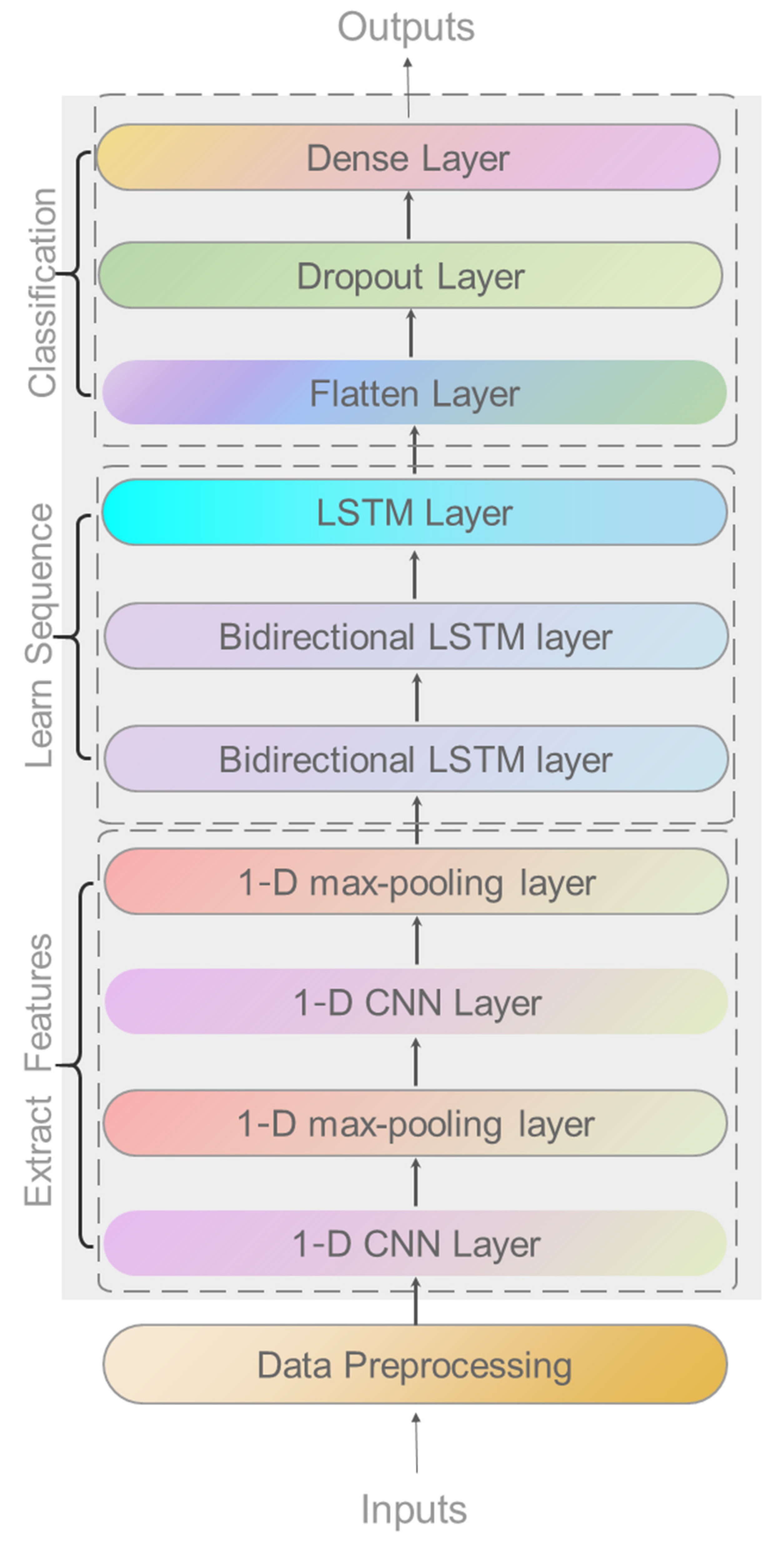
In our research, we used a combination of a convolutional neural network (CNN) and bi-directional long short-term memory (Bi-LSTM) to train our proposed SafeNet model (Figure 4). The model’s architecture comprises one-dimensional (1D) convolutional layers, a 1D Bi-LSTM structural layer, and a fully connected (FC) block. For feature extraction from the input data, the SafeNet model employs CNN layers, which are combined with Bi-LSTMs to facilitate sequence prediction. SafeNet accesses subsequences of main sequence as blocks, collects features from each block, and then transfers extracted features to the LSTM layer for interpretation. To enable the CNN model to read each subsequence in the window, the entire CNN model is wrapped in a Time Distributed layer. The extracted features are then flattened and provided to the Bi-LSTM layer for reading, and further features are extracted. The 1D convolutional layers are utilized to extract data features in concept, and then Bi-LSTM structures are employed to optimize feature extraction in sequential data. Finally, the classification probability is calculated using an FC layer. The loss function is categorical cross-entropy, and the optimization is performed using the Adam method [31]. For more details on the SafeNet network architecture, please refer to Text S4 (Supplementary Materials).
The proposed model was developed in TensorFlow 2.0 with the Keras (v. 2.3.0) interface [32]. To facilitate fast training, all models were trained on a server equipped with two Intel Xeon E5-2650 v4 CPUs, 128 GB of RAM, and an NVIDIA GeForce RTX 2080 Ti graphics processing unit (GPU) [33]. Owing to the sensitivity of the proposed method to the chosen parameters, Bayesian hyperparameter tuning was utilized to determine the optimal settings [34] and was developed using the Hyperopt Python package [35]. The negative of the F-measure (F1) was utilized as the objective function’s return value (loss) in this procedure. The procedure optimized hyperparameters based on their capacity to minimize an objective function by constructing a probability model based on the results of previous evaluations. Consequently, this model can be expected to perform better with fewer iterations than the random or grid searches would require. Table S1 (Supplementary Materials) summarizes the search space for SafeNet’s important parameters. Each model was assigned a maximum of 100 iterations. DataSet S1 (Supplementary Materials) provides the hyperparametric optimization trial results for all the datasets used to train the SafeNet model and other benchmarking classifiers.
3.3. Performance Evaluation
Datasets utilized in this study were often class unbalanced, with the number of samples representing the non-seismic class being much greater than the number of samples representing the other classes [36]. In this situation, a simple classifier that predicted each sample as the majority class could achieve a high level of accuracy; thus, the total classification accuracy was insufficient to assess performance. As a result, we used the F-measure (F1) to evaluate model performance, which considers the correct classification of each class to be equally important. The F1 score is a metric that considers precision and recall. This is often referred to as the harmonic mean of both. Consequently, class imbalance was addressed by weighting the various classes according to their sample proportions. The Matthews correlation coefficient (MCC) [37], which emphasizes positives in samples, was also employed in this study. The specific formulas for the performance metrics such as F1 score and MCC are defined in Text S3 (Supplementary Materials).
Furthermore, in this study, receiver operating characteristic (ROC) curves, which are plots of the true positive rate versus the false positive rate, were employed to assess the output quality of the classifier’s performance. The ROC curve is often used in binary classification settings to assess the output of a classifier. To extend the ROC curve and ROC area for multiclass classification, the output was binarized, and one ROC curve was drawn and used to evaluate classifier quality per class. In addition, we computed the area under the ROC curve, known as the AUC, which was used to compare various models. In this study, higher AUC values were regarded as better methods for identifying ionospheric perturbations prior to earthquakes.
Finally, to visually illustrate the classification performance of each class, ternary probability diagrams and confusion matrices were used to depict the probability distributions for each input class in the test data, as well as the distribution of predicted and actual values.
Five state-of-the-art machine learning models were benchmarked for the study task: gradient boosting machine [38], deep neural network (DNN) [39], random forest [40], CNN [41], and LSTM [42] models. These methods were implemented in Python (v. 3.6) with scikit-learn (v. 0.20.0) and Keras (v. 2.3.0). Because the explored models are sensitive to parameter selection, we chose parameters that yielded the best performance using Bayesian hyperparameter tuning, as described above. After the optimal parameters were determined for each method, the performances of the different methods were compared.
4. Results
We used the Swarm dataset to train the proposed SafeNet model directly, which had been split into the training and test sets. Initially, we configured the data with 60 consecutive observations as the input sequence length, a spatial window centered at the epicenter, a deviation of the Dobrovolsky radius [29], and nighttime data in the initial configuration, because there is no universal standard for lengths of the input sequence and the spatial window (DataSet 01 in Table 1). In our study, we consistently considered data from 15 days before to 5 days after every earthquake and set it as the temporal window.
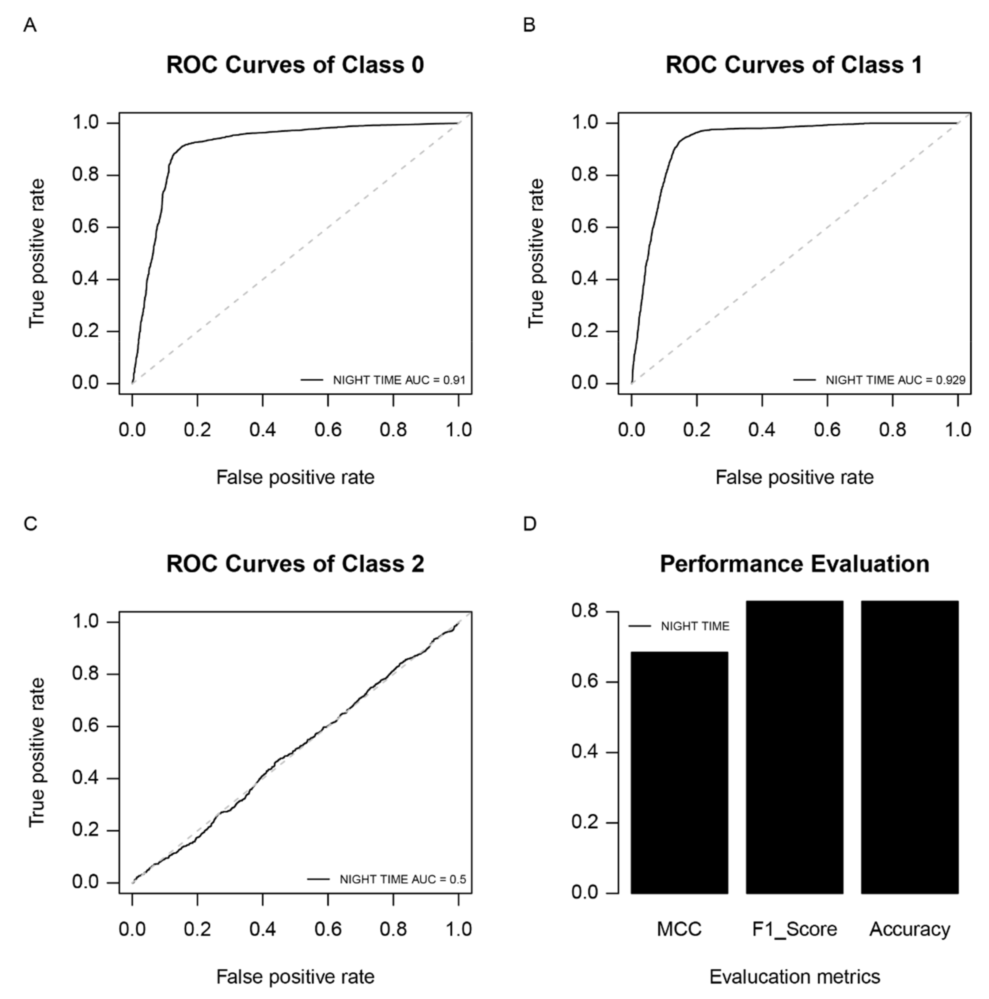
As illustrated in Figure 5, the ROC curves were used as a performance measure because they represent relative trade-offs between true positives (benefits) and false positives (costs) for each class, and the performance of the model utilizing nighttime data is shown. The AUC values of classes 0 and 1 were both greater than 0.9 (Figure 5A,B), indicating that the model can roughly distinguish time series related to earthquakes and non-seismic events, but the AUC of class 2 was only 0.50 (Figure 5C), indicating that the accuracy of the model in identifying space weather such as magnetic storms was low. This may be due to the fact that class 2 was trained with a lower number of samples, causing the model to fail to extract the features of the class. Figure 5D depicts the MCC, F1 score, and accuracy bar plot curves, which represent the overall performance of the model. The findings were similar to those implied by the ROC curves, showing that the model could distinguish earthquakes from non-seismic and space events to some degree. In general, the performance of the model based on the initial setup was reasonable, but not remarkable. As a result, we investigated whether combining datasets with various temporal and geographic characteristics, as well as alternative models, might provide an improved performance.
4.1. Considering Various Input Sequence Lengths
To further investigate whether the SafeNet method can identify pre-earthquake disturbances with varying input sequence lengths and whether it can improve performance, datasets with the following input sequence length of consecutive observations were created (Table 1): 80 (DataSet 02), 70 (DataSet 03), 50 (DataSet 04), and 40 (DataSet 05) consecutive observations.
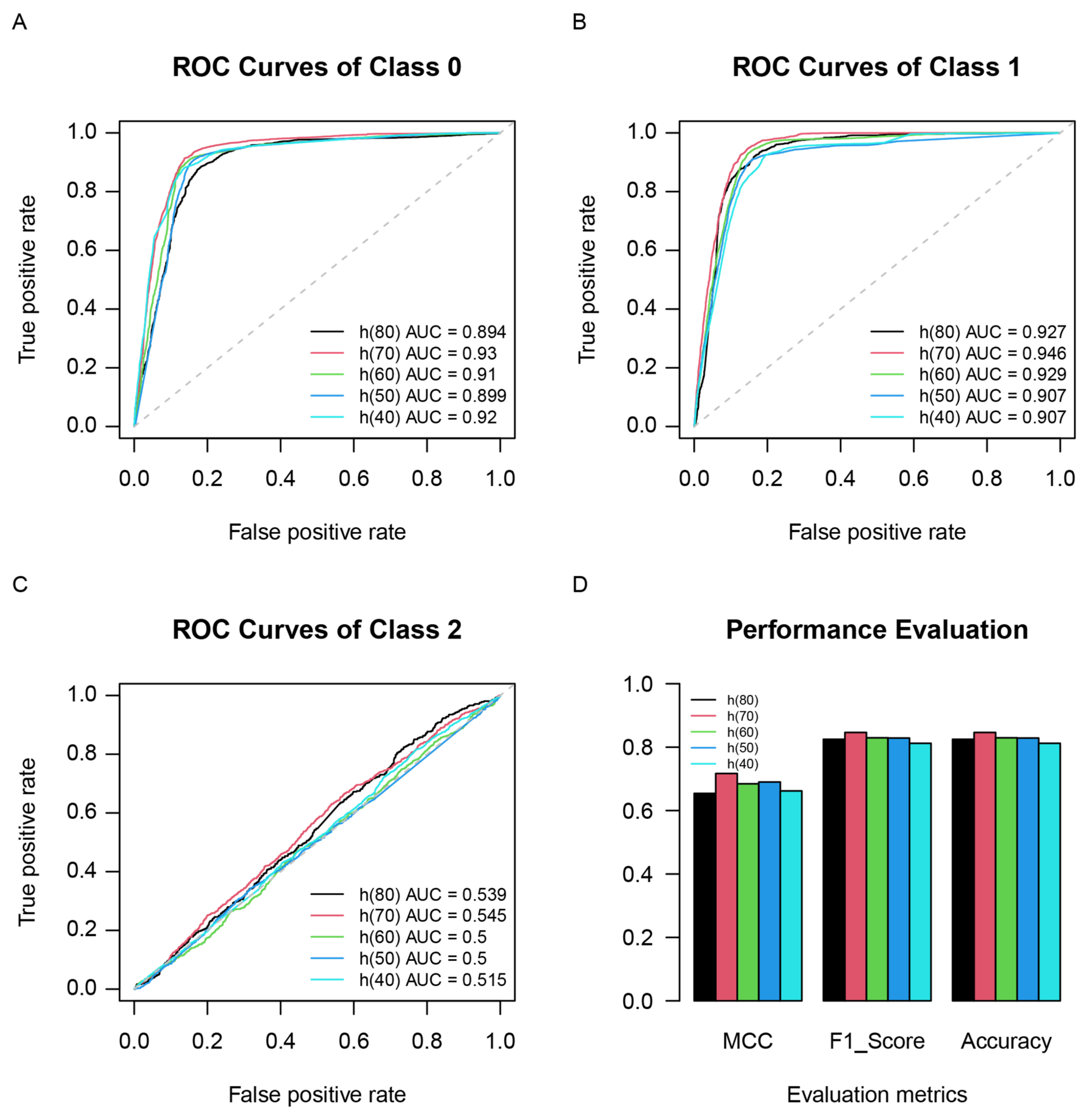
Figure 6 depicts the ROC curves and MCC, F1 score, and accuracy bar plot curves for the datasets with varying input sequence lengths. Table 2 lists the classification performance metrics achieved using the SafeNet. In Table 2, it is revealed that the overall F1 scores vary from 0.812 to 0.846, and the MCC varies from 0.654 to 0.717 for various datasets; these values are also shown in Figure 6D, which shows a performance comparison of the results. It was illustrated that as the input sequence length fluctuated, the performance of the model changed as well, and the optimal performance was achieved using the dataset with an input sequence length of 70 consecutive observations (DataSet 03). According to the ROC curves shown in Figure 6A–C, SafeNet also offered a reasonable performance for each class when DataSet 03 was used. Based on these results, we could conclude that the length of the input sequence had an influence on the performance of the SafeNet model, and that the best performance was achieved with an input sequence of 70 consecutive observations.
4.2. Data Comparing Nighttime Versus Daytime
The data acquisition time may affect the identification of pre-earthquake electromagnetic perturbations. To illustrate the effect of data collection time, a daytime dataset (Dataset 06 in Table 1) was created. As shown in Figure 7 and Table 2, SafeNet’s performance was compared using benchmark datasets generated during the day and night. We evaluated the model’s performance using the AUC, MCC, F1, and accuracy indicators.
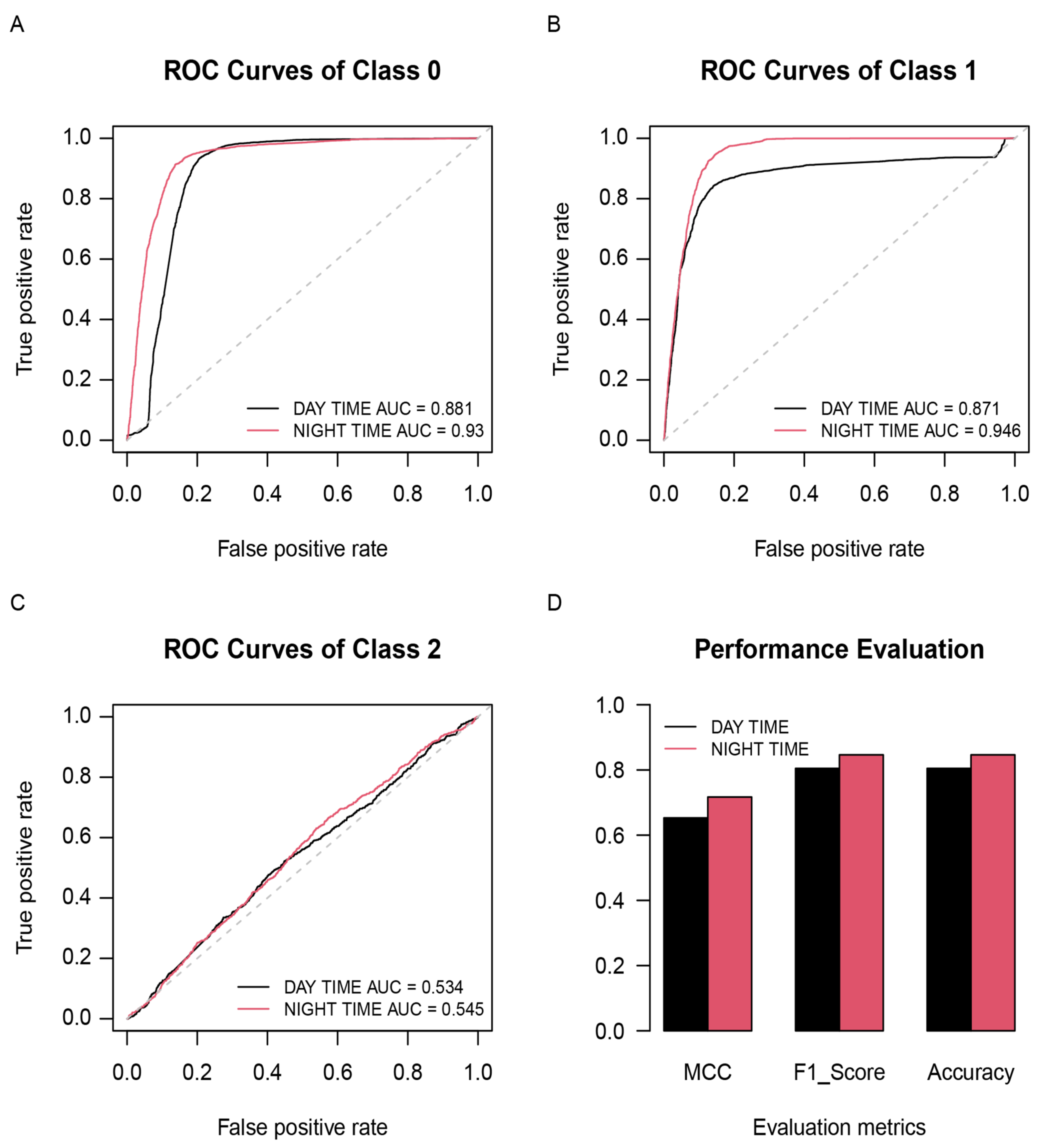
For the same spatial and temporal features, we found that using the nighttime datasets (Dataset 03 in Table 1) resulted in a higher classification performance than using the daytime dataset (Table 2). SafeNet’s ROC curves for both datasets are given in Figure 7A–C, and we can observe that the AUC curve for nighttime data is somewhat higher than that for daytime data, with approximately 5.7%, 8.6%, and 2.1% increases in AUC for the three classes, respectively. When all classes were taken into account, SafeNet’s F1 score improved from 0.805 to 0.846 when nighttime data were used, compared to daytime data, and MCC improved by 9.8% (Table 2).
Figure 7D compares the MCC, F1 score, and accuracy values between the daytime and nighttime data, revealing that the nighttime data performed slightly better than the daytime data. One reason for this may be that, because ionospheric conditions are typically more disturbed during the day, identifying seismic electromagnetic effects is more difficult, which may reflect a small number of significant changes in daytime data. This finding is supported by other research on statistical results of electromagnetic disturbances caused by earthquakes [16,43,44,45,46].
4.3. Considering Various Spatial Windows
SafeNet worked effectively for a circular region centered at the epicenter with a Dobrovolsky radius (DataSet 03). To further investigate the impact of various spatial windows on the performance of the model, satellite datasets with spatial windows of 3° (DataSet 07), 5° (DataSet 08), 7° (DataSet 09), and 10° (DataSet 10) were created (Table 1).
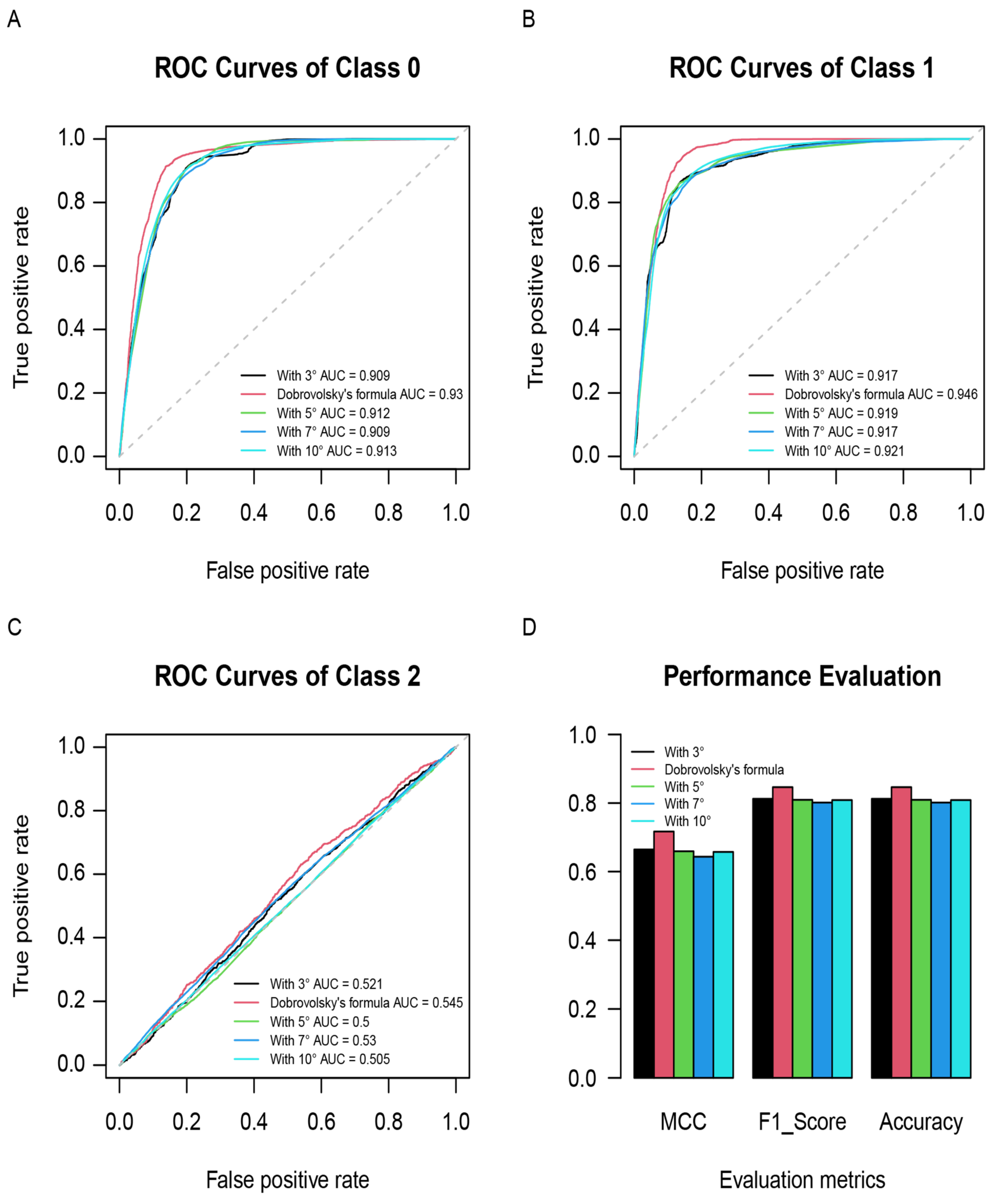
Table 2 details the SafeNet’s performance on the five datasets, and Figure 8 illustrates the ROC and MCC curves, F1 score, and accuracy bar plot curves. SafeNet performed best when the dataset was used with the spatial window radius given by Dobrovolsky’s formula (DataSet 03), with an F1 score of 0.846 and an MCC of 0.717. Comparing the results from Figure 8D and Table 2 shows that an improvement in the overall performance was not achieved with larger spatial windows. This tendency is also evident in the ROC curves in Figure 8A–C, where DataSet 03 had the highest AUC value of the datasets. Though the cause for these findings is unclear, it could be that a disturbance moving upward from the Earth’s surface alters the ionosphere’s properties geometrically, and the radius of the affected area matches the radius calculated using Dobrovolsky’s formula. In addition, among the cases with different sizes of the preparation area (DataSet 07–10), it is the smaller ones that show the best performance. This could be due to the fact that there are more earthquakes with a smaller magnitude (i.e., 4.8–5.0) than those with a larger magnitude.
4.4. Considering the Magnitude of the Earthquake
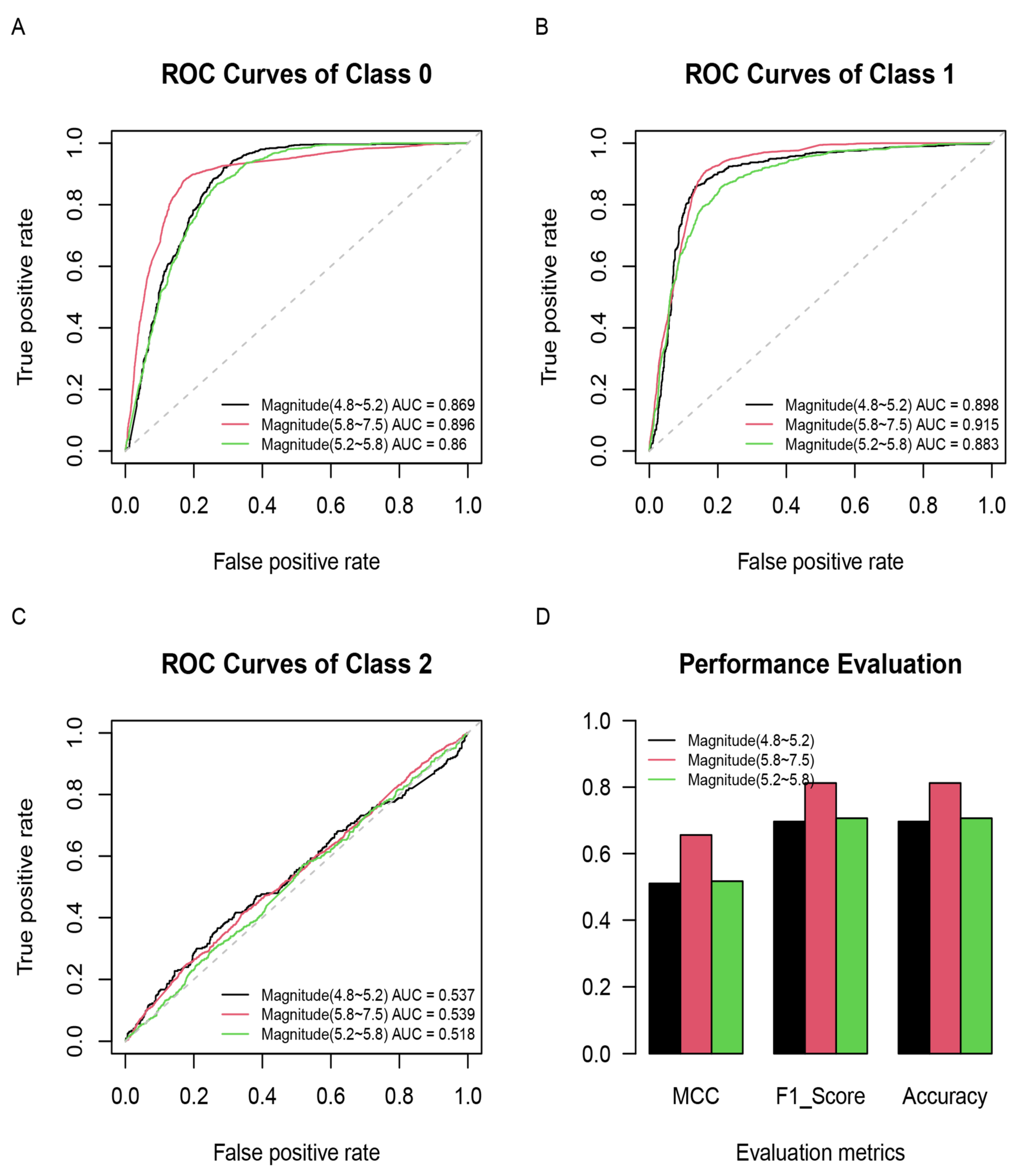
It is well known that earthquake magnitude may play an active role in the identification of pre-earthquake perturbations. Therefore, to demonstrate the influence of magnitudes, we divided earthquakes into groups of three—5136 earthquakes with magnitudes between 4.8 and 5.2, 2793 earthquakes with magnitudes between 5.2 and 5.8, and 853 earthquakes with magnitudes between 5.8 and 7.5, and the corresponding datasets were created: DataSet 11, DataSet 12, and DataSet 13 (Table 1).
Table 2 illustrates the performance of the SafeNet model for the three datasets. As shown in Figure 9, the model had similar performance over the three datasets; for example, the AUC of class 0 and class 1 on all three datasets using the SafeNet method was above 0.86, and the F1 score ranged from 0.697 to 0.812, which suggests that the SafeNet model provides a satisfactory performance in discriminating electromagnetic pre-earthquake perturbations on the datasets with different magnitudes. Moreover, it can be concluded from Table 2 and Figure 9 that the larger the magnitude, the better the classification performance. This is also in line with the reality.
4.5. Considering Unbalanced Datasets
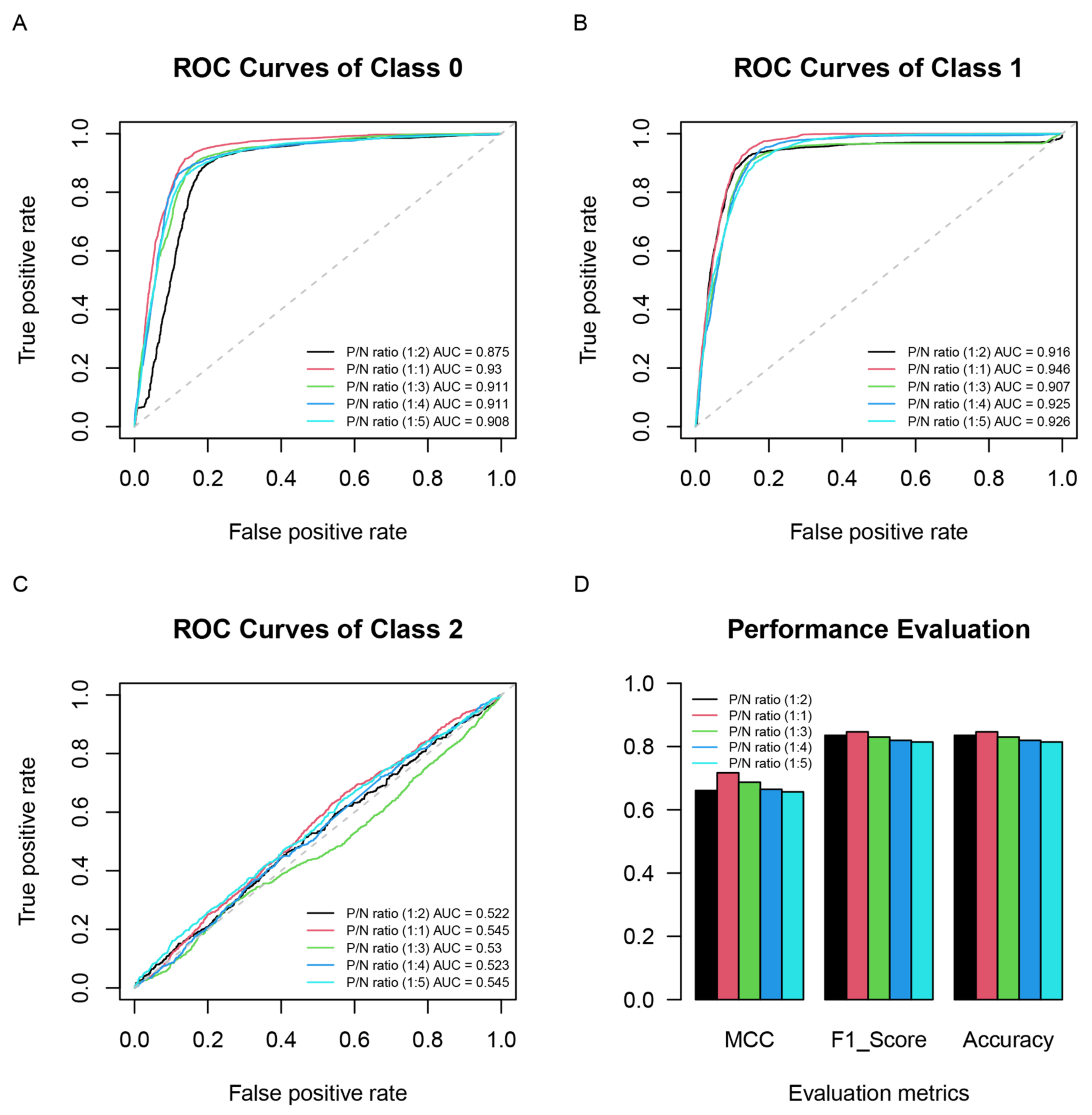
The actual situation of earthquake issues is usually highly unbalanced, and it is obvious that non-earthquake datasets are always significantly larger than earthquake datasets. To test the real performance of the SafeNet model on unbalanced datasets as well as to investigate whether our proposed method could be applied to earthquake anomaly identification on unbalanced datasets, datasets with the positive to negative ratio of 1:2 (DataSet 14), 1:3 (DataSet 15), 1:4 (DataSet 16), and 1:5 (DataSet 17) were generated (shown in Table 1).
Table 2 illustrates the performance of the SafeNet model on five datasets (including DataSet 03). Although the method performs most effectively on the dataset with a positive to negative ratio of 1:1 (DataSet 03), the overall performance is similar on the five datasets; for instance, the proposed method has F1 scores around 0.83 (ranging from 0.814 to 0.846) as well as MCC values ranging from 0.661 to 0.717. Figure 10 shows the ROC curves for all three classes, together with a comparison of the performance metrics; we also observed a similar trend of our proposed method’s performance on the five datasets, which suggests that the SafeNet model achieves a good performance for pre-seismic perturbation identification on the unbalanced dataset. Although the five unbalanced datasets are different, these results show that our method is less sensitive on the positive to negative ratio, and our method can be used to identify possible electromagnetic preseismic perturbations on an unbalanced dataset, which suggests that it could provide a good realistic performance.
4.6. Comparative Analysis of Other Classifiers
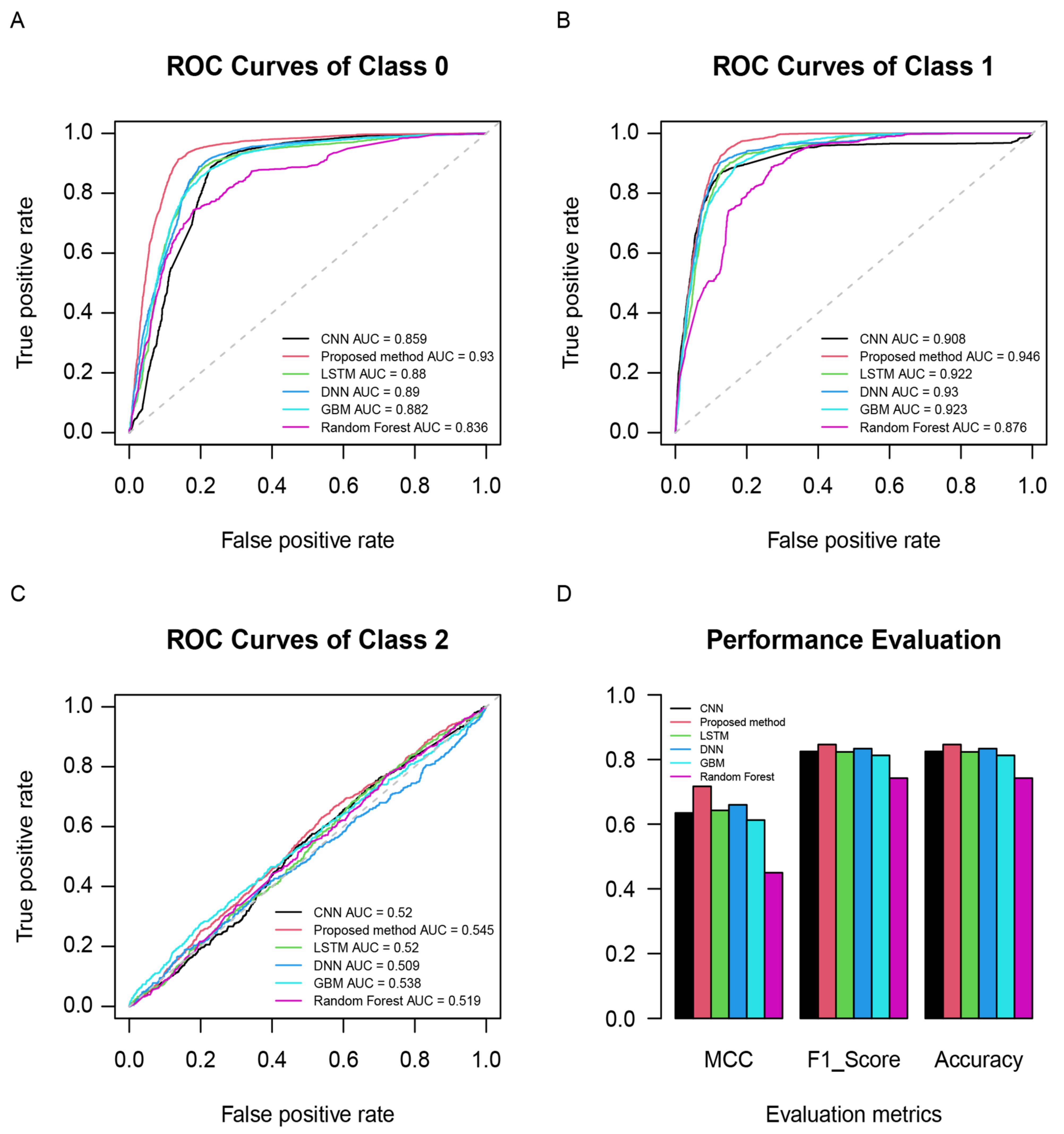
Table 2 and Figure 11 report the performance of our SafeNet model with five other benchmarking classifiers for DataSet 03. The performance of the existing methods ranged from F1 = 0.742 to 0.846 and MCC = 0.450 to 0.717. However, SafeNet had the best performance, improving MCC by 8.6% over that of the next-best DNN model. Figure 11A–C compares the ROC curves obtained for the SafeNet model with those of the five other classifiers, and SafeNet again demonstrated the best performance with a 4.6% improvement in AUC for class 0, a 1.7% improvement for class 1, and a 7.1% improvement for class 2 over the second-best DNN model.
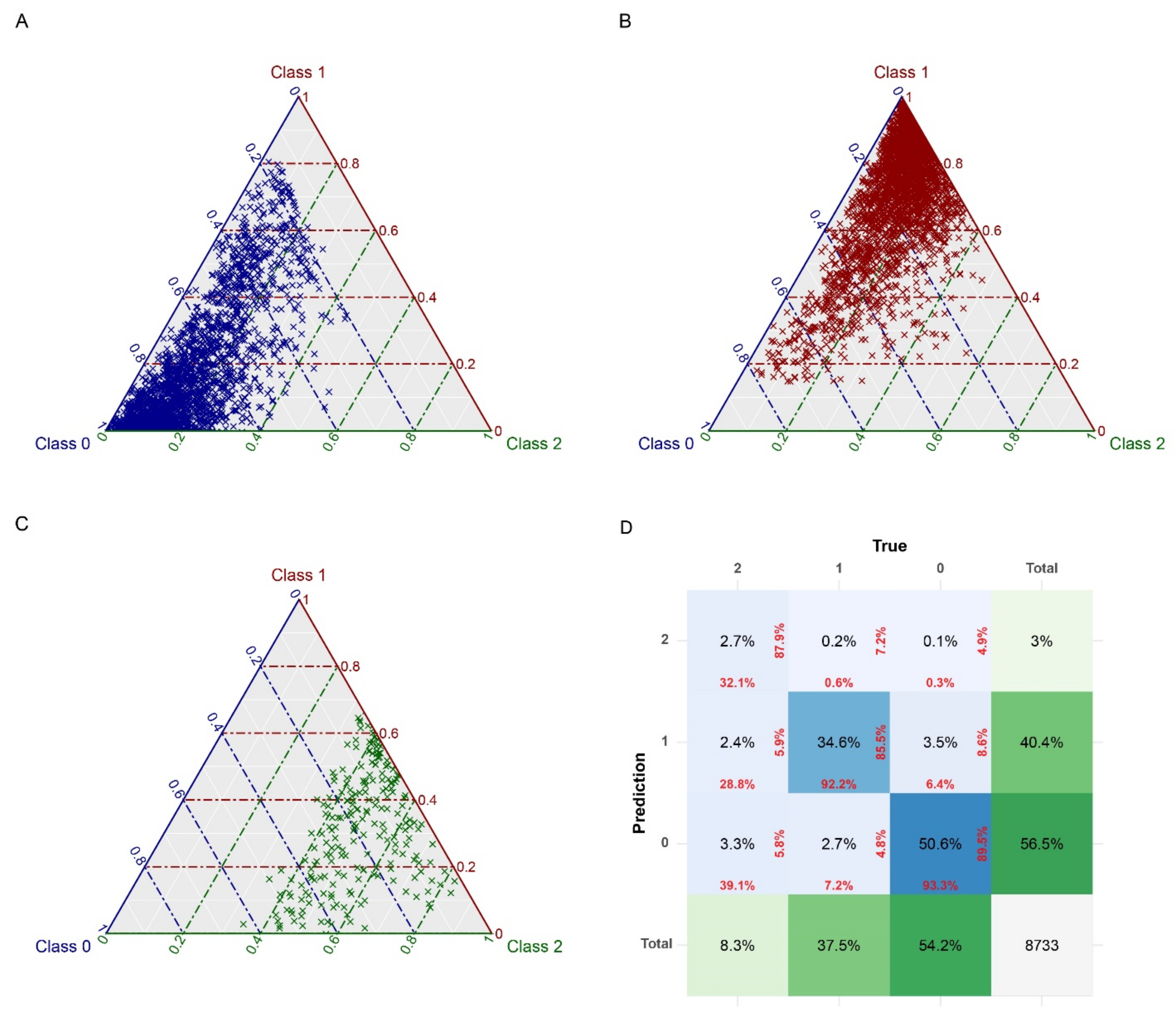
To further confirm the performance of SafeNet, ternary probability diagrams and a confusion matrix were used to indicate the distribution of the predicted and true values and to allow for more profound insight into the classification performance of the model. Figure 12 shows the ternary probability diagrams and confusion matrix for the three classes obtained from the SafeNet model. Ternary probability diagrams allow for a qualitative evaluation of classification results. From Figure 12A–C as a whole, most of the samples in class 0 and class 1 were correctly predicted, and classes predicted by SafeNet could be classified into the correct classes, while the performance of class 2 was slightly worse, with some samples having a prediction probability concentrated around 0.5. The confusion matrices shown in Figure 12D quantitatively present the prediction accuracy for each class, with the correct prediction accuracy for class 0, class 1, and class 2 of 89.5%, 85.5%, and 87.9%, respectively. In general, SafeNet provides a good classification performance for identifying seismic signals and space weather events from Swarm satellite data.
5. Discussions
Several studies have investigated the physical mechanisms of ionospheric pre-earthquake perturbations [47,48,49,50,51]. Perhaps the most widely accepted hypotheses regarding these mechanisms were presented by Pulinets, et al. [52] and Kuo, Lee, and Huba [27], who proposed complex lithosphere–atmosphere–ionosphere coupling as the physical basis for the generation of short-term earthquake precursors. Specifically, the lower crust and upper mantle generate gases such as radon (Rn) at lithostatic pressure during the buildup to an earthquake, and this gas could form large-scale domains in the rock. When reaching a certain vertical extent, these gas domains could become hydrostatically unstable and force their way upward through the lithosphere. Rapid lithospheric degassing can be expected to trigger several atmospheric processes near the Earth’s surface, leading to changes in air conductivity and, therefore, changes to the near-ground atmospheric electric field. It is known that, as a part of the global electric circuit, the ionosphere immediately reacts to changes in near-ground electric properties, and an electric field induced within the ionosphere can cause ion drift and irregularities in electron concentrations. To better understand the mechanisms of ionospheric pre-earthquake perturbations, Freund [53] performed a series of experiments on a loaded rock and found that stress activation of p-hole charge carriers in the Earth’s crust led to regional positive ground potential. In these scenarios, ionospheric perturbations are expected.
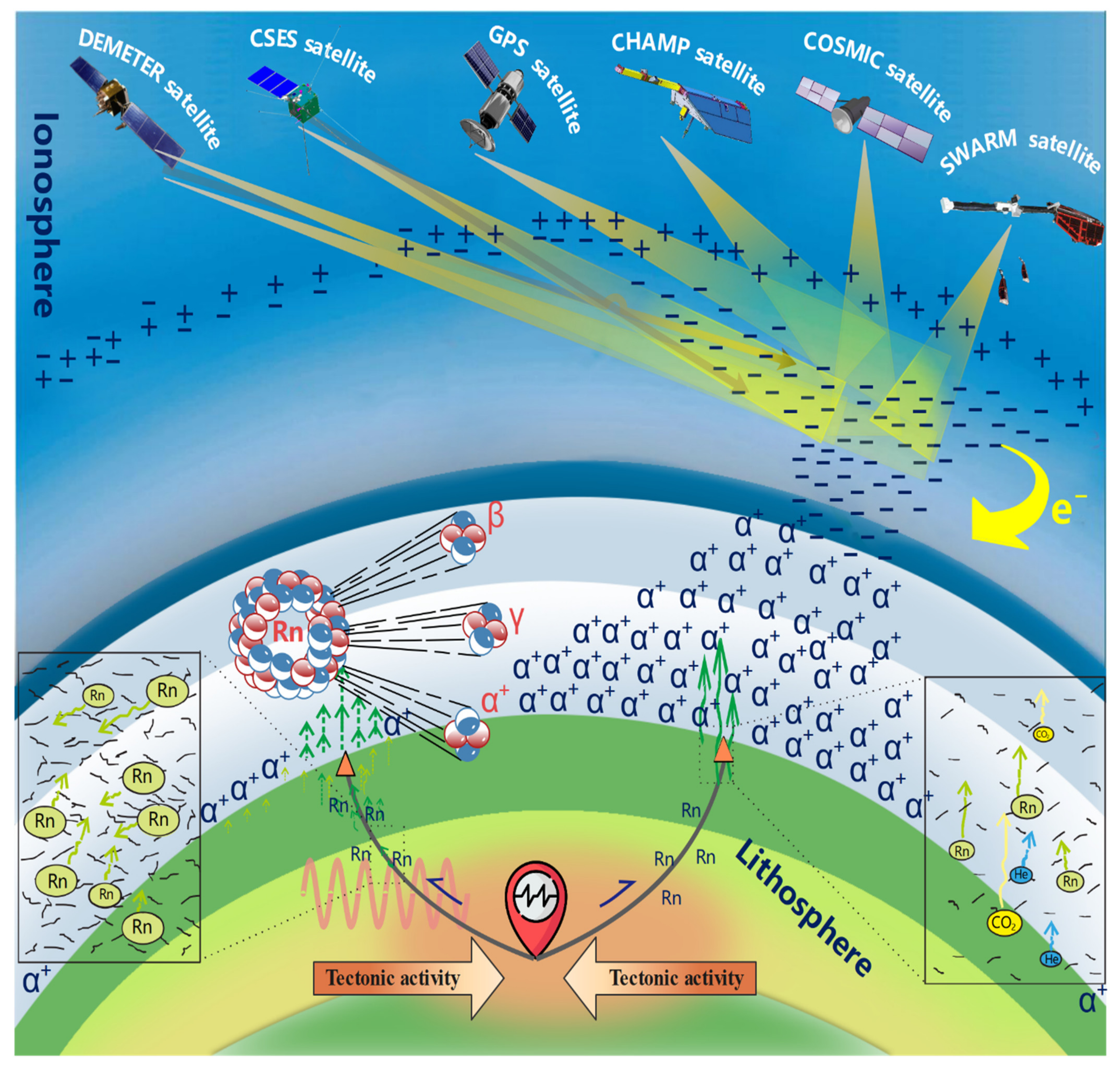
Crustal strain measurements often fail to detect any unusual changes before earthquakes [54], and the measurement of Rn gas content is among the most reported earthquake precursors [55,56]. Moreover, continuous monitoring of soil gas radon and water radon concentrations along with the Amritsar (Punjab, India) seismic zone correlation showed that the amplitude of radon gas anomalies was positively correlated with earthquake magnitude [57]. In addition, recent studies revealed a significant decrease in radon concentration within continuous measurements of radon concentration in the atmosphere before the 2018 earthquake in northern Osaka, Japan [58] and peculiar changes in radon concentration in the atmosphere two months before the 1995 Kobe earthquake in Japan [59]; Fu et al. [60] studied the radon gas anomalies in northern and northeastern Taiwan before the earthquake and observed a significant increase in soil radon concentration from a few days to a few weeks before the earthquake. Finally, it is reasonable that the amount of emitted radon could depend on the rupture length of the fault, that is, the magnitude of the seismic event. This study considers Rn gas emissions as the most reasonable result to be initially triggered by an earthquake. Because Rn decay can emit alpha particles, we propose a new hypothesis to explain the physical mechanisms of earthquake-induced ionospheric perturbations, as schematically depicted in Figure 13. In this hypothesis, various crustal movements in the pre-earthquake stage lead to rock fragmentation, melting, mineral dissolution, or phase change, and daughter isotopes of some radioactive parent isotopes retained in certain minerals or rocks are released in large quantities. In this situation, the Rn gas content in the area near the epicenter is abnormal before the earthquake, and furthermore the Rn gas decays quickly (half-life is about 3.8 days). During Rn decay, many alpha particles are released. The energy of an alpha particle is 5.2 MeV, and the ionization energy required by an atmospheric molecule is 32 eV. Therefore, one alpha particle is sufficient to generate 150,000 pairs of positive and negative ions, thereby creating an excess of positive airborne ions near the Earth’s surface.
Because pre-earthquake field ionization occurs over relatively wide areas, we suggest that the positively charged air bubble expands owing to its internal electrostatic repulsion. Furthermore, as the prevailing electric field has an acceleration effect on positive airborne ions relative to the Earth’s surface, the only direction of the airborne ions is upward. Therefore, many airborne ions would rise rapidly and shorten the vertical potential difference between the Earth’s surface and the ionosphere. In response, the ionospheric plasma would be expected to polarize, causing the electrons located at the bottom of the ionosphere to be pulled downward. Thus, the physical properties of the ionosphere respond to changes in the vertical distribution of electrons and ions in the ionospheric plasma. In this way, it will result in a vertical electric field, E. The electric field pushes upward current flow from the atmosphere into the ionosphere. The injected current could result in the ionosphere being subjected to an enforced electric field. The perpendicular component of the electric field causes plasma E × B motion, which results in fluctuations in the ionosphere’s density [27,61].
Moreover, the ionospheric anomalies before and after the earthquake could be positive or negative, and the probability of positive and negative perturbations is almost the same [62]. Simulations of anomalous electric fields show that if the anomalous electric field is westward, then the density enhancement occurs at the equator and the electron density decreases upward at the polarities [62]. If there is an eastward anomalous electric field, the positive and negative anomaly positions will be opposite. According to our knowledge, the anomalous electric field will be significantly different from one earthquake or different times of the same earthquake, so both positive and negative anomalies could be observed before and after the earthquake. In addition, Yao, et al. [63] also found that both positive and negative anomalies could occur before the earthquake by analyzing the GIM TEC of all Ms 7.0+ earthquakes in 2010. In addition, Zhao et al. studied the Wenchuan earthquake and also found that some of the GPS station data near the epicenter showed positive anomalies and some showed negative anomalies [64].
In the development of earthquake mechanisms at this stage, more experimental and actual evidence of radon gas generation in pressurized rocks is needed because it can provide a reasonable explanation for the uncertain relationship between pre-seismic electromagnetic anomalies and actual seismic events. In addition, in this endeavor, we suggest setting up ground-based observations of DC electric fields or using VLF noise anomalies to monitor the electrical activity of the atmosphere and lithosphere.
6. Conclusions
This study proposed the SafeNet deep learning framework for pre-earthquake ionospheric perturbation identification. SafeNet was trained and tested using 9017 independent earthquakes of magnitude 4.8 and above that occurred from April 2014 to April 2020, and the corresponding plasma and magnetic field data from the Swarm A satellite for about 6 years. The results indicated that electromagnetic pre-earthquake data within a circular region centered on the epicenter and with a radius given by the Dobrovolsky formula, with a model input window size of 70 consecutive points and nighttime sequence data, yielded the best performance in discriminating electromagnetic pre-earthquake perturbations, with an F1 score of 0.846 and an MCC value of 0.717. The study also concluded that the larger the magnitude of the earthquake, the better the performance of the SafeNet model in identifying possible pre-earthquake ionospheric anomalies. The results also suggest that the SafeNet model achieves a good performance for probable pre-seismic perturbation identification on the unbalanced dataset. In addition, based on constraints from this study, we proposed a new hypothesis on the physical mechanisms of earthquake-induced ionospheric perturbations.
In order to have a better understanding of the lithosphere, atmosphere, and ionosphere coupling mechanisms, to study pre-earthquake anomalies using electromagnetic satellites, the analysis of the spatial-temporal correlation of multi-sphere and multi-parameters by a remote sensing technique before earthquakes occur has become a hot research topic in recent years. However, it is difficult to match the different parameters and data of each sphere in both time and space. The existing multi-parameter earthquake studies are mainly focused on specific earthquakes or specific remote sensing parameters, have not sufficiently considered the other remote-sensing parameters of other spheres, and have not formed a complete chain of multi-parameter correlation analyses. The deep learning technology can overpass such limitations, combining the remote sensing parameters of multiple spheres in time and space and carrying out the analysis based on a consistent spatial-temporal framework, which could provide global earthquake cases and effectively explain the earthquake coupling mechanism models, and also expand the current tools for earthquake monitoring, providing new perspectives for earthquake prediction.
Supplementary Materials
The following are available online at https://www.mdpi.com/article/10.3390/rs13245033/s1, Text S1. Swarm Alpha nighttime tracks before the M7.9 Sumatra 2 March 2016 earthquake. Text S2. Swarm Alpha nighttime tracks before the M7.8 Ecuador 16 April 2016 earthquake. Text S3. Performance metrics. Text S4. The SafeNet model structure. Figure S25. The flowchart of the proposed deep learning framework. Table S1. Search space of parameters for the SafeNet model.
Author Contributions
Conceptualization, X.Z. and X.S.; data curation, P.X.; investigation, D.M., A.D.S., and X.Z.; methodology, P.X. and A.D.S.; project administration, A.D.S. and X.S.; software, P.X.; visualization, P.X. and D.M.; writing—original draft, P.X.; writing—review and editing, D.M., A.D.S., X.Z., and X.S. All authors have read and agreed to the published version of the manuscript.
Funding
This work is supported by the Special Fund of the Institute of Earthquake Forecasting, China Earthquake Administration (Grant No. 2021IEF0706, 2020IEF0510, 2021IEF0708) and funded by the National Key R&D Program of China under Grant No. 2018YFC1503505; Pianeta Dinamico-Working Earth (Italian Ministry of University and Research) and Limadou-Science+ (Italian Space Agency) Projects; National Natural Science Foundation of China (Grant number: 41974084); the China Postdoctoral Science Foundation (Grant number: 2021M691190).
Institutional Review Board Statement
Not applicable.
Informed Consent Statement
Not applicable.
Data Availability Statement
The Swarm data can be downloaded from the ESA Swarm FTP and HTTP Server swarm-diss.eo.esa.int. The Kp indices used in this paper were provided by the World Data Center for Geomagnetism, Kyoto (http://wdc.kugi.kyoto-u.ac.jp/wdc/Sec3.html).
Conflicts of Interest
The authors declare no conflict of interest.
References
- Moore, G.W. Magnetic Disturbances preceding the 1964 Alaska Earthquake. Nature 1964, 203, 508–509. [Google Scholar] [CrossRef]
- Davies, K.; Baker, D.M. Ionospheric effects observed around the time of the Alaskan earthquake of March 28, 1964. J. Geophys. Res. 1965, 70, 2251–2253. [Google Scholar] [CrossRef]
- Parrot, M.; Li, M. Demeter results related to seismic activity. URSI Radio Sci. Bull. 2015, 2015, 18–25. [Google Scholar]
- De Santis, A.; Balasis, G.; Pavón-Carrasco, F.J.; Cianchini, G.; Mandea, M. Potential earthquake precursory pattern from space: The 2015 Nepal event as seen by magnetic Swarm satellites. Earth Planet. Sci. Lett. 2017, 461, 119–126. [Google Scholar] [CrossRef] [Green Version]
- Marchetti, D.; De Santis, A.; D’Arcangelo, S.; Poggio, F.; Piscini, A.; Campuzano, S.A.; De Carvalho, W.V.J.O. Pre-earthquake chain processes detected from ground to satellite altitude in preparation of the 2016–2017 seismic sequence in Central Italy. Remote Sens. Environ. 2019, 229, 93–99. [Google Scholar] [CrossRef]
- Marchetti, D.; De Santis, A.; Campuzano, S.A.; Soldani, M.; Piscini, A.; Sabbagh, D.; Cianchini, G.; Perrone, L.; Orlando, M. Swarm Satellite Magnetic Field Data Analysis Prior to 2019 Mw = 7.1 Ridgecrest (California, USA) Earthquake. Geosciences 2020, 10, 502. [Google Scholar] [CrossRef]
- Zhu, K.; Fan, M.; He, X.; Marchetti, D.; Li, K.; Yu, Z.; Chi, C.; Sun, H.; Cheng, Y. Analysis of Swarm Satellite Magnetic Field Data Before the 2016 Ecuador (Mw = 7.8) Earthquake Based on Non-negative Matrix Factorization. Front. Earth Sci. 2021, 9, 1976. [Google Scholar] [CrossRef]
- Christodoulou, V.; Bi, Y.; Wilkie, G. A tool for Swarm satellite data analysis and anomaly detection. PLoS ONE 2019, 14, e0212098. [Google Scholar] [CrossRef] [PubMed]
- Akhoondzadeh, M.; De Santis, A.; Marchetti, D.; Piscini, A.; Jin, S. Anomalous seismo-LAI variations potentially associated with the 2017 Mw = 7.3 Sarpol-e Zahab (Iran) earthquake from Swarm satellites, GPS-TEC and climatological data. Adv. Space Res. 2019, 64, 143–158. [Google Scholar] [CrossRef]
- Marchetti, D.; Akhoondzadeh, M. Analysis of Swarm satellites data showing seismo-ionospheric anomalies around the time of the strong Mexico (Mw = 8.2) earthquake of 08 September 2017. Adv. Space Res. 2018, 62, 614–623. [Google Scholar] [CrossRef]
- Zhu, K.; Li, K.; Fan, M.; Chi, C.; Yu, Z. Precursor Analysis Associated With the Ecuador Earthquake Using Swarm A and C Satellite Magnetic Data Based on PCA. IEEE Access 2019, 7, 93927–93936. [Google Scholar] [CrossRef]
- Akhoondzadeh, M.; De Santis, A.; Marchetti, D.; Piscini, A.; Cianchini, G. Multi precursors analysis associated with the powerful Ecuador (MW = 7.8) earthquake of 16 April 2016 using Swarm satellites data in conjunction with other multi-platform satellite and ground data. Adv. Space Res. 2018, 61, 248–263. [Google Scholar] [CrossRef] [Green Version]
- Parrot, M. Statistical analysis of automatically detected ion density variations recorded by DEMETER and their relation to seismic activity. Ann. Geophys. 2012, 55. [Google Scholar] [CrossRef]
- Yan, R.; Parrot, M.; Pinçon, J.-L. Statistical Study on Variations of the Ionospheric Ion Density Observed by DEMETER and Related to Seismic Activities. J. Geophys. Res. Space Phys. 2017, 122, 12,421–12,429. [Google Scholar] [CrossRef] [Green Version]
- Li, M.; Shen, X.; Parrot, M.; Zhang, X.; Zhang, Y.; Yu, C.; Yan, R.; Liu, D.; Lu, H.; Guo, F.; et al. Primary Joint Statistical Seismic Influence on Ionospheric Parameters Recorded by the CSES and DEMETER Satellites. J. Geophys. Res. Space Phys. 2020, 125. [Google Scholar] [CrossRef]
- De Santis, A.; Marchetti, D.; Pavon-Carrasco, F.J.; Cianchini, G.; Perrone, L.; Abbattista, C.; Alfonsi, L.; Amoruso, L.; Campuzano, S.A.; Carbone, M.; et al. Precursory worldwide signatures of earthquake occurrences on Swarm satellite data. Sci. Rep. 2019, 9, 20287. [Google Scholar] [CrossRef] [PubMed] [Green Version]
- Marchetti, D.; De Santis, A.; Jin, S.; Campuzano, S.A.; Cianchini, G.; Piscini, A. Co-Seismic Magnetic Field Perturbations Detected by Swarm Three-Satellite Constellation. Remote Sens. 2020, 12, 1166. [Google Scholar] [CrossRef] [Green Version]
- Bergen, K.J.; Johnson, P.A.; de Hoop, M.V.; Beroza, G.C. Machine learning for data-driven discovery in solid Earth geoscience. Science 2019, 363, eaau0323. [Google Scholar] [CrossRef] [PubMed]
- Rouet-Leduc, B.; Hulbert, C.; Johnson, P.A. Continuous chatter of the Cascadia subduction zone revealed by machine learning. Nat. Geosci. 2018, 12, 75–79. [Google Scholar] [CrossRef]
- Ross, Z.E.; Trugman, D.T.; Hauksson, E.; Shearer, P.M. Searching for hidden earthquakes in Southern California. Science 2019, 364, 767–771. [Google Scholar] [CrossRef] [Green Version]
- Xiong, P.; Long, C.; Zhou, H.; Battiston, R.; Zhang, X.; Shen, X. Identification of Electromagnetic Pre-Earthquake Perturbations from the DEMETER Data by Machine Learning. Remote Sens. 2020, 12, 3643. [Google Scholar] [CrossRef]
- Xiong, P.; Tong, L.; Zhang, K.; Shen, X.; Battiston, R.; Ouzounov, D.; Iuppa, R.; Crookes, D.; Long, C.; Zhou, H. Towards advancing the earthquake forecasting by machine learning of satellite data. Sci. Total Environ. 2021, 771, 145256. [Google Scholar] [CrossRef] [PubMed]
- Xiong, P.; Long, C.; Zhou, H.; Battiston, R.; De Santis, A.; Ouzounov, D.; Zhang, X.; Shen, X. Pre-Earthquake Ionospheric Perturbation Identification Using CSES Data via Transfer Learning. Front. Environ. Sci. 2021, 9, 9255. [Google Scholar] [CrossRef]
- Olsen, N.; Friis-Christensen, E.; Floberghagen, R.; Alken, P.; Beggan, C.D.; Chulliat, A.; Doornbos, E.; da Encarnação, J.T.; Hamilton, B.; Hulot, G.; et al. The Swarm Satellite Constellation Application and Research Facility (SCARF) and Swarm data products. Earth Planets Space 2013, 65, 1189–1200. [Google Scholar] [CrossRef]
- Friis-Christensen, E.; Lühr, H.; Hulot, G. Swarm: A constellation to study the Earth’s magnetic field. Earth Planets Space 2006, 58, 351–358. [Google Scholar] [CrossRef] [Green Version]
- Pinheiro, K.J.; Jackson, A.; Finlay, C.C. Measurements and uncertainties of the occurrence time of the 1969, 1978, 1991, and 1999 geomagnetic jerks. Geochem. Geophys. Geosyst. 2011, 12. [Google Scholar] [CrossRef]
- Kuo, C.L.; Lee, L.C.; Huba, J.D. An improved coupling model for the lithosphere-atmosphere-ionosphere system. J. Geophys. Res. Space Phys. 2014, 119, 3189–3205. [Google Scholar] [CrossRef]
- De Santis, A.; Marchetti, D.; Spogli, L.; Cianchini, G.; Pavón-Carrasco, F.J.; Franceschi, G.D.; Di Giovambattista, R.; Perrone, L.; Qamili, E.; Cesaroni, C.; et al. Magnetic Field and Electron Density Data Analysis from Swarm Satellites Searching for Ionospheric Effects by Great Earthquakes: 12 Case Studies from 2014 to 2016. Atmosphere 2019, 10, 371. [Google Scholar] [CrossRef] [Green Version]
- Dobrovolsky, I.; Zubkov, S.; Miachkin, V. Estimation of the size of earthquake preparation zones. Pure Appl. Geophys. 1979, 117, 1025–1044. [Google Scholar] [CrossRef]
- Spogli, L.; Sabbagh, D.; Regi, M.; Cesaroni, C.; Perrone, L.; Alfonsi, L.; Di Mauro, D.; Lepidi, S.; Campuzano, S.A.; Marchetti, D.; et al. Ionospheric Response Over Brazil to the August 2018 Geomagnetic Storm as Probed by CSES-01 and Swarm Satellites and by Local Ground-Based Observations. J. Geophys. Res. Space Phys. 2021, 126. [Google Scholar] [CrossRef]
- Kingma, D.P.; Ba, J. Adam: A method for stochastic optimization. arXiv 2014, arXiv:1412.6980. [Google Scholar]
- Abadi, M.; Barham, P.; Chen, J.; Chen, Z.; Davis, A.; Dean, J.; Devin, M.; Ghemawat, S.; Irving, G.; Isard, M. Tensorflow: A system for large-scale machine learning. In Proceedings of the 12th USENIX symposium on operating systems design and implementation (OSDI 16), Savannah, GA, USA, 2–4 November 2016; pp. 265–283. [Google Scholar]
- Oh, K.-S.; Jung, K. GPU implementation of neural networks. Pattern Recognit. 2004, 37, 1311–1314. [Google Scholar] [CrossRef]
- Snoek, J.; Larochelle, H.; Adams, R.P. Practical bayesian optimization of machine learning algorithms. In Proceedings of the Advances in Neural Information Processing Systems, Lake Tahoe, CA, USA, 3–8 December 2012; pp. 2951–2959. [Google Scholar]
- Bergstra, J.; Yamins, D.; Cox, D.D. Making a science of model search: Hyperparameter optimization in hundreds of dimensions for vision architectures. In Proceedings of the 30th International Conference on International Conference on Machine Learning, Atlanta, GA, USA, 16–21 June 2013; Volume 28, pp. I-115–I-123. [Google Scholar]
- Japkowicz, N.; Stephen, S. The class imbalance problem: A systematic study. Intell. Data Anal. 2002, 6, 429–449. [Google Scholar] [CrossRef]
- Matthews, B.W. Comparison of the predicted and observed secondary structure of T4 phage lysozyme. Biochim. Biophys. Acta 1975, 405, 442–451. [Google Scholar] [CrossRef]
- Friedman, J.H. Greedy Function Approximation: A Gradient Boosting Machine. Ann. Stat. 2001, 29, 1189–1232. [Google Scholar] [CrossRef]
- LeCun, Y.; Bengio, Y.; Hinton, G. Deep learning. Nature 2015, 521, 436–444. [Google Scholar] [CrossRef] [PubMed]
- Geurts, P.; Ernst, D.; Wehenkel, L. Extremely randomized trees. Mach. Learn. 2006, 63, 3–42. [Google Scholar] [CrossRef] [Green Version]
- Krizhevsky, A.; Sutskever, I.; Hinton, G.E. Imagenet classification with deep convolutional neural networks. In Proceedings of the Advances in Neural Information Processing Systems, Lake Tahoe, CA, USA, 3–8 December 2012; pp. 1097–1105. [Google Scholar]
- Hochreiter, S.; Schmidhuber, J. Long short-term memory. Neural Comput. 1997, 9, 1735–1780. [Google Scholar] [CrossRef]
- Němec, F.; Santolík, O.; Parrot, M.; Berthelier, J.J. Spacecraft observations of electromagnetic perturbations connected with seismic activity. Geophys. Res. Lett. 2008, 35. [Google Scholar] [CrossRef] [Green Version]
- Němec, F.; Santolík, O.; Parrot, M. Decrease of intensity of ELF/VLF waves observed in the upper ionosphere close to earthquakes: A statistical study. J. Geophys. Res. Space Phys. 2009, 114. [Google Scholar] [CrossRef]
- Píša, D.; Němec, F.; Parrot, M.; Santolík, O. Attenuation of electromagnetic waves at the frequency ~1.7 kHz in the upper ionosphere observed by the DEMETER satellite in the vicinity of earthquakes. Ann. Geophys. 2012, 55, 157–163. [Google Scholar] [CrossRef]
- Píša, D.; Němec, F.; Santolík, O.; Parrot, M.; Rycroft, M. Additional attenuation of natural VLF electromagnetic waves observed by the DEMETER spacecraft resulting from preseismic activity. J. Geophys. Res. Space Phys. 2013, 118, 5286–5295. [Google Scholar] [CrossRef] [Green Version]
- Pulinets, S.; Ouzounov, D. Lithosphere–Atmosphere–Ionosphere Coupling (LAIC) model—An unified concept for earthquake precursors validation. J. Asian Earth Sci. 2011, 41, 371–382. [Google Scholar] [CrossRef]
- Ouzounov, D.; Pulinets, S.; Liu, J.-Y.; Hattori, K.; Han, P. Multiparameter Assessment of Pre-Earthquake Atmospheric Signals. Pre-Earthq. Process. 2018, 339–359. [Google Scholar] [CrossRef]
- Freund, F.T.; Heraud, J.A.; Centa, V.A.; Scoville, J. Mechanism of unipolar electromagnetic pulses emitted from the hypocenters of impending earthquakes. Eur. Phys. J. Spec. Top. 2021, 230, 47–65. [Google Scholar] [CrossRef]
- Wu, L.-X.; Qin, K.; Liu, S.-J. GEOSS-Based Thermal Parameters Analysis for Earthquake Anomaly Recognition. Proc. IEEE 2012, 100, 2891–2907. [Google Scholar] [CrossRef]
- Hayakawa, M.; Kasahara, Y.; Nakamura, T.; Muto, F.; Horie, T.; Maekawa, S.; Hobara, Y.; Rozhnoi, A.A.; Solovieva, M.; Molchanov, O.A. A statistical study on the correlation between lower ionospheric perturbations as seen by subionospheric VLF/LF propagation and earthquakes. J. Geophys. Res. Space Phys. 2010, 115. [Google Scholar] [CrossRef]
- Pulinets, S.A.; Ouzounov, D.P.; Karelin, A.V.; Davidenko, D.V. Physical bases of the generation of short-term earthquake precursors: A complex model of ionization-induced geophysical processes in the lithosphere-atmosphere-ionosphere-magnetosphere system. Geomagn. Aeron. 2015, 55, 521–538. [Google Scholar] [CrossRef]
- Freund, F.T. Pre-earthquake signals—Part I: Deviatoric stresses turn rocks into a source of electric currents. Nat. Hazards Earth Syst. Sci. 2007, 7, 535–541. [Google Scholar] [CrossRef] [Green Version]
- Soter, S. Macroscopic seismic anomalies and submarine pockmarks in the Corinth–Patras rift, Greece. Tectonophysics 1999, 308, 275–290. [Google Scholar] [CrossRef]
- Riggio, A.; Santulin, M. Earthquake forecasting: A review of radon as seismic precursor. Boll. Di Geofis. Teor. Ed Appl. 2015, 56. [Google Scholar]
- Gold, T.; Soter, S. Fluid ascent through the solid lithosphere and its relation to earthquakes. Pure Appl. Geophys. 1985, 122, 492–530. [Google Scholar] [CrossRef]
- Kumar, A.; Walia, V.; Singh, S.; Bajwa, B.S.; Dhar, S.; Yang, T.F. Earthquake precursory studies at Amritsar Punjab, India using radon measurement techniques. Int. J. Phys. Sci. 2013, 7, 5669–5677. [Google Scholar]
- Muto, J.; Yasuoka, Y.; Miura, N.; Iwata, D.; Nagahama, H.; Hirano, M.; Ohmomo, Y.; Mukai, T. Preseismic atmospheric radon anomaly associated with 2018 Northern Osaka earthquake. Sci. Rep. 2021, 11, 7451. [Google Scholar] [CrossRef] [PubMed]
- Omori, Y.; Nagahama, H.; Yasuoka, Y.; Muto, J. Radon degassing triggered by tidal loading before an earthquake. Sci. Rep. 2021, 11, 4092. [Google Scholar] [CrossRef]
- Fu, C.-C.; Lee, L.-C.; Yang, T.F.; Lin, C.-H.; Chen, C.-H.; Walia, V.; Liu, T.-K.; Ouzounov, D.; Giuliani, G.; Lai, T.-H.; et al. Gamma Ray and Radon Anomalies in Northern Taiwan as a Possible Preearthquake Indicator around the Plate Boundary. Geofluids 2019, 2019, 1–14. [Google Scholar] [CrossRef] [Green Version]
- Kuo, C.L.; Huba, J.D.; Joyce, G.; Lee, L.C. Ionosphere plasma bubbles and density variations induced by pre-earthquake rock currents and associated surface charges. J. Geophys. Res. Space Phys. 2011, 116. [Google Scholar] [CrossRef] [Green Version]
- Liu, J.; Wan, W.; Zhou, C.; Zhang, X.; Liu, Y.; Shen, X. A study of the ionospheric disturbances associated with strong earthquakes using the empirical orthogonal function analysis. J. Asian. Earth Sci. 2019, 171, 225–232. [Google Scholar] [CrossRef]
- Yao, Y.B.; Chen, P.; Zhang, S.; Chen, J.J.; Yan, F.; Peng, W.F. Analysis of pre-earthquake ionospheric anomalies before the global M = 7.0+ earthquakes in 2010. Nat. Hazards Earth Syst. Sci. 2012, 12, 575–585. [Google Scholar] [CrossRef] [Green Version]
- Zhao, B.; Wang, M.; Yu, T.; Xu, G.; Wan, W.; Liu, L. Ionospheric total electron content variations prior to the 2008 Wenchuan Earthquake. Int. J. Remote Sens. 2010, 31, 3545–3557. [Google Scholar] [CrossRef]
Figure 1.
Swarm Alpha satellite nighttime track 26 of 15 February 2016 acquired 16 days before the M7.9 Sumatra 2016 earthquake. Panels D, E, and F show magnetic X, Y, and Z components residual after derivate and cubic-spline removal (MASS method; De Santis et al. [4]). Panels A, B, and C provide the FAST Fourier Transform of the residual of X, Y, and Z, respectively. Panel G shows the logarithm of electron density, with a 10-degree polynomial fit as a red line. The pixels that present Ne values that significantly deviate from the fit are identified as blue stars and they are potential anomalies as defined by NeLOG in De Santis et al. [28]. The map in panel H shows the epicenter of the earthquake by a green star and its preparation area defined by Dobrovolsky et al. [29] as a yellow circle. In the title of the figure, the satellite (A for Alpha, B for Bravo, and C for Charlie), date, track number (counted daily), and time in local and UTC times of the center of the track are indicated. The values of the geomagnetic indexes Dst and ap at the track acquisition time are also provided, and in the second line of title the number of flagged samples are provided together with the total number of samples in the track.

Figure 2.
Swarm Alpha satellite nighttime track 3 of 7 April 2016 acquired 9 days before the M7.8 Ecuador 2016 earthquake. The description of the subfigures is the same as in Figure 1.
Figure 2.
Swarm Alpha satellite nighttime track 3 of 7 April 2016 acquired 9 days before the M7.8 Ecuador 2016 earthquake. The description of the subfigures is the same as in Figure 1.

Figure 3.
Sequence labeling after data segmentation using a sliding window. Consecutive observations of used parameters are segmented by non-overlapping sliding windows. T is the window’s length. Non-seismic data are marked as 0 (class 0), seismic data are marked as 1 (class 1), and data with a Kp index greater than 3 are marked as 2 (class 2), regardless of whether they are associated with an earthquake.

Figure 4.
The bottom-up network framework architecture of the SafeNet model. 1-D CNN: One-dimensional convolutional neural network; Dropout: drop-out layer; Bidirectional LSTM: bidirectional long short-term memory layer. “Flatten” and “Dense” are the names of the functional layers.
Figure 4.
The bottom-up network framework architecture of the SafeNet model. 1-D CNN: One-dimensional convolutional neural network; Dropout: drop-out layer; Bidirectional LSTM: bidirectional long short-term memory layer. “Flatten” and “Dense” are the names of the functional layers.

Figure 5.
Receiver operating characteristic (ROC) curves showing SafeNet’s performance for (A) class 0, (B) class 1, and (C) class 2 utilizing nighttime data. (D) Matthews correlation coefficient (MCC), F1 score, and accuracy bar plot curves illustrating the model’s performance with nighttime data.
Figure 5.
Receiver operating characteristic (ROC) curves showing SafeNet’s performance for (A) class 0, (B) class 1, and (C) class 2 utilizing nighttime data. (D) Matthews correlation coefficient (MCC), F1 score, and accuracy bar plot curves illustrating the model’s performance with nighttime data.

Figure 6.
Comparing model performance using ROC curves for (A) class 0, (B) class 1, and (C) class 2 with window sizes of 40, 50, 60, 70, and 80. (D) Bar plots of the MCC, F1 score, and accuracy at various window sizes. We use the letter h to define the window size, and the numbers in brackets represent the specific size.

Figure 7.
The ROC curves comparing model performance in nighttime vs. daytime data for (A) class 0, (B) class 1, and (C) class 2. (D) Comparison of model performance for nighttime and daytime data using bar plots of MCC, F1 score, and accuracy.
Figure 7.
The ROC curves comparing model performance in nighttime vs. daytime data for (A) class 0, (B) class 1, and (C) class 2. (D) Comparison of model performance for nighttime and daytime data using bar plots of MCC, F1 score, and accuracy.

Figure 8.
The ROC curves comparing model performance for (A) class 0, (B) class 1, and (C) class 2 with various spatial window radii of 3°, Dobrovolsky’s formula, 5°, 7°, and 10°. (D) Bar plots showing the MCC, F1 score, and accuracy of the results.
Figure 8.
The ROC curves comparing model performance for (A) class 0, (B) class 1, and (C) class 2 with various spatial window radii of 3°, Dobrovolsky’s formula, 5°, 7°, and 10°. (D) Bar plots showing the MCC, F1 score, and accuracy of the results.

Figure 9.
The ROC curves comparing model performance for (A) class 0, (B) class 1, and (C) class 2 of earthquakes with magnitudes between 4.8 and 5.2, earthquakes with magnitudes between 5.2 and 5.8, and earthquakes with magnitudes between 5.8 and 7.5. (D) Bar graphs displaying the MCC, F1 score, and accuracy.

Figure 10.
The ROC curves comparing model performance for (A) class 0, (B) class 1, and (C) class 2 of datasets with the positive to negative ratio of 1:1 (DataSet 3), 1:2 (DataSet 14), 1:3 (DataSet 15), 1:4 (DataSet 16), and 1:5 (DataSet 17). (D) Bar graphs displaying the MCC, F1 score, and accuracy.

Figure 11.
The ROC curves comparing the proposed method, gradient boosting machine (GBM), deep neural network (DNN), random forest (RF), convolutional neural network (CNN), and long short-term memory (LSTM) models for (A) class 0, (B) class 1, and (C) class 2. (D) The MCC, F1 score, and accuracy bar plot curves.

Figure 12.
Ternary probability diagrams illustrating the findings of SafeNet on the test data for (A) class 0, (B) class 1, and (C) class 2. Class 0 is represented by blue crosses, class 1 by red crosses, and class 2 by green crosses; the color of the cross indicates the actual class, and the distance projected from each cross to the class axis represents the probability of that class in the model prediction. (D) Matrix of confusion illustrating the distribution of estimated and actual values. Each tile’s center contains the normalized count (overall percentage) in black text. Column percentages are shown at the bottom of each tile, while row percentages are displayed on the right (both in red text). The sum tiles on the plot’s right and bottom (in shades of green) indicate the overall distribution of predictions and targets. Note that the color intensity is proportional to the number of counts.

Figure 13.
The proposed physical mechanisms of ionospheric perturbations induced by earthquakes. A large area of rock is broken and torn before the earthquake, after which a channel is opened to continuously release radon gas to generate radioactive decay. A gas bubble, laden with positive airborne ions generated during the process of radon decay at the ground-to-air interface, expands upward through the atmosphere, carrying up the Earth’s ground potential and eliciting a polarization response in the ionosphere. This leads to a redistribution of the electrons at the lower edge of the ionosphere and thus modifies its physical properties. Thus, the satellite will receive anomalous signals from the ionosphere.


Table 1.
Datasets with different features generated using Swarm data.
| DataSet | Night/Daytime | Spatial Feature | Input Sequence Length | Earthquake Magnitude/No. of Real Earthquakes/Positive to Negative Ratio |
|---|---|---|---|---|
| DataSet 01 | Nighttime | with its center at the epicenter and the Dobrovolsky radius | 60 continuous points | above 4.8/9017/1:1 |
| DataSet 02 | Nighttime | with its center at the epicenter and the Dobrovolsky radius | 80 continuous points | above 4.8/9017/1:1 |
| DataSet 03 | Nighttime | with its center at the epicenter and the Dobrovolsky radius | 70 continuous points | above 4.8/9017/1:1 |
| DataSet 04 | Nighttime | with its center at the epicenter and the Dobrovolsky radius | 50 continuous points | above 4.8/9017/1:1 |
| DataSet 05 | Nighttime | with its center at the epicenter and the Dobrovolsky radius | 40 continuous points | above 4.8/9017/1:1 |
| DataSet 06 | Daytime | with its center at the epicenter and the Dobrovolsky radius | 70 continuous points | above 4.8/9017/1:1 |
| DataSet 07 | Nighttime | with its center at the epicenter and a deviation of 3° | 70 continuous points | above 4.8/9017/1:1 |
| DataSet 08 | Nighttime | with its center at the epicenter and a deviation of 5° | 70 continuous points | above 4.8/9017/1:1 |
| DataSet 09 | Nighttime | with its center at the epicenter and a deviation of 7° | 70 continuous points | above 4.8/9017/1:1 |
| DataSet 10 | Nighttime | with its center at the epicenter and a deviation of 10° | 70 continuous points | above 4.8/9017/1:1 |
| DataSet 11 | Nighttime | with its center at the epicenter and the Dobrovolsky radius | 70 continuous points | 4.8~5.2/5136/1:1 |
| DataSet 12 | Nighttime | with its center at the epicenter and the Dobrovolsky radius | 70 continuous points | 5.2~5.8/2793/1:1 |
| DataSet 13 | Nighttime | with its center at the epicenter and the Dobrovolsky radius | 70 continuous points | 5.8~7.5/853/1:1 |
| DataSet 14 | Nighttime | with its center at the epicenter and the Dobrovolsky radius | 70 continuous points | above 4.8/9017/1:2 |
| DataSet 15 | Nighttime | with its center at the epicenter and the Dobrovolsky radius | 70 continuous points | above 4.8/9017/1:3 |
| DataSet 16 | Nighttime | with its center at the epicenter and the Dobrovolsky radius | 70 continuous points | above 4.8/9017/1:4 |
| DataSet 17 | Nighttime | with its center at the epicenter and the Dobrovolsky radius | 70 continuous points | above 4.8/9017/1:5 |
Table 2.
Performance comparison of SafeNet and benchmark classifiers on different datasets.
| Method | DataSet | MCC | F1 | Accuracy | AUC of Class 0 | AUC of Class 1 | AUC of Class 2 |
|---|---|---|---|---|---|---|---|
| SafeNet | DataSet 01 | 0.684 | 0.830 | 0.830 | 0.910 | 0.929 | 0.500 |
| DataSet 02 | 0.654 | 0.825 | 0.825 | 0.894 | 0.927 | 0.539 | |
| DataSet 03 | 0.717 | 0.846 | 0.846 | 0.931 | 0.946 | 0.545 | |
| DataSet 04 | 0.690 | 0.829 | 0.829 | 0.899 | 0.907 | 0.500 | |
| DataSet 05 | 0.662 | 0.812 | 0.812 | 0.920 | 0.907 | 0.515 | |
| DataSet 06 | 0.653 | 0.805 | 0.805 | 0.881 | 0.871 | 0.534 | |
| DataSet 07 | 0.665 | 0.812 | 0.812 | 0.909 | 0.917 | 0.521 | |
| DataSet 08 | 0.659 | 0.809 | 0.809 | 0.912 | 0.919 | 0.500 | |
| DataSet 09 | 0.644 | 0.801 | 0.801 | 0.909 | 0.917 | 0.531 | |
| DataSet 10 | 0.657 | 0.809 | 0.809 | 0.913 | 0.921 | 0.505 | |
| DataSet 11 | 0.510 | 0.697 | 0.697 | 0.869 | 0.898 | 0.537 | |
| DataSet 12 | 0.517 | 0.706 | 0.706 | 0.860 | 0.883 | 0.518 | |
| DataSet 13 | 0.656 | 0.812 | 0.812 | 0.896 | 0.915 | 0.539 | |
| DataSet 14 | 0.661 | 0.835 | 0.835 | 0.875 | 0.916 | 0.522 | |
| DataSet 15 | 0.687 | 0.830 | 0.830 | 0.911 | 0.907 | 0.530 | |
| DataSet 16 | 0.665 | 0.819 | 0.819 | 0.911 | 0.925 | 0.523 | |
| DataSet 17 | 0.657 | 0.814 | 0.814 | 0.908 | 0.926 | 0.545 | |
| CNN | DataSet 03 | 0.635 | 0.825 | 0.825 | 0.859 | 0.908 | 0.520 |
| LSTM | DataSet 03 | 0.643 | 0.824 | 0.824 | 0.880 | 0.923 | 0.520 |
| DNN | DataSet 03 | 0.660 | 0.834 | 0.834 | 0.890 | 0.930 | 0.509 |
| GBM | DataSet 03 | 0.613 | 0.813 | 0.813 | 0.882 | 0.923 | 0.538 |
| RF | DataSet 03 | 0.450 | 0.742 | 0.742 | 0.836 | 0.876 | 0.519 |
Publisher’s Note: MDPI stays neutral with regard to jurisdictional claims in published maps and institutional affiliations. |
© 2021 by the authors. Licensee MDPI, Basel, Switzerland. This article is an open access article distributed under the terms and conditions of the Creative Commons Attribution (CC BY) license (https://creativecommons.org/licenses/by/4.0/).
Share and Cite
MDPI and ACS Style
Xiong, P.; Marchetti, D.; De Santis, A.; Zhang, X.; Shen, X. SafeNet: SwArm for Earthquake Perturbations Identification Using Deep Learning Networks. Remote Sens. 2021, 13, 5033. https://doi.org/10.3390/rs13245033
AMA Style
Xiong P, Marchetti D, De Santis A, Zhang X, Shen X. SafeNet: SwArm for Earthquake Perturbations Identification Using Deep Learning Networks. Remote Sensing. 2021; 13(24):5033. https://doi.org/10.3390/rs13245033
Chicago/Turabian StyleXiong, Pan, Dedalo Marchetti, Angelo De Santis, Xuemin Zhang, and Xuhui Shen. 2021. "SafeNet: SwArm for Earthquake Perturbations Identification Using Deep Learning Networks" Remote Sensing 13, no. 24: 5033. https://doi.org/10.3390/rs13245033
Note that from the first issue of 2016, this journal uses article numbers instead of page numbers. See further details here.