
Estimating Leaf Area Index with Dynamic Leaf Optical Properties
by
 , and
, and
Hu Zhang
1,2 ,
,
Jing Li
1,2,*, 
Qinhuo Liu
1,2, 
Yadong Dong
1,
Songze Li
1,2,
Zhaoxing Zhang
1,
Xinran Zhu
1,2,
Liangyun Liu
3 and
Jing Zhao
1
1
State Key Laboratory of Remote Sensing Science, Aerospace Information Research Institute, Chinese Academy of Sciences and Beijing Normal University, Beijing 100101, China
2
College of Resources and Environment, University of Chinese Academy of Sciences, Beijing 100190, China
3
Key Laboratory of Digital Earth, Aerospace Information Research Institute, Chinese Academy of Sciences, Beijing 100094, China
*
Author to whom correspondence should be addressed.
Remote Sens. 2021, 13(23), 4898; https://doi.org/10.3390/rs13234898
Submission received: 8 November 2021
/
Revised: 30 November 2021
/
Accepted: 1 December 2021
/
Published: 2 December 2021
(This article belongs to the Section Remote Sensing in Agriculture and Vegetation)
Abstract
:Leaf area index (LAI) plays an important role in models of climate, hydrology, and ecosystem productivity. The physical model-based inversion method is a practical approach for large-scale LAI inversion. However, the ill-posed inversion problem, due to the limited constraint of inaccurate input parameters, is the dominant source of inversion errors. For instance, variables related to leaf optical properties are always set as constants or have large ranges, instead of the actual leaf reflectance of pixel vegetation in the current model-based inversions. This paper proposes to estimate LAI with the actual leaf optical property of pixels, calculated from the leaf chlorophyll content (Chlleaf) product, using a three-dimensional stochastic radiative transfer model (3D-RTM)-based, look-up table method. The parameter characterizing leaf optical properties in the 3D-RTM-based LAI inversion algorithm, single scattering albedo (SSA), is calculated with the Chlleaf product, instead of setting fixed values across a growing season. An algorithm to invert LAI with the dynamic SSA of the red band (SSAred) is proposed. The retrieval index (RI) increases from less than 42% to 100%, and the RMSE decreases to less than 0.28 in the simulations. The validation results show that the RMSE of the dynamic SSA decreases from 1.338 to 0.511, compared with the existing 3D-RTM-based LUT algorithm. The overestimation problem under high LAI conditions is reduced.
1. Introduction
The leaf area index (LAI), defined as the one-sided green leaf area per unit ground area in broadleaf canopies [1,2], is a key parameter in models of climate, meteorology, hydrology, biogeochemistry, and ecosystem productivity to characterize vegetation canopy structure [3,4,5,6]. Over the last decades, different methods to retrieve LAI from remote sensing data have been developed, and a series of global LAI products have been released [7]. The methods to estimate LAI can be classified into three major types: the empirical transfer method [8], the physical model inversion method [9,10], and the machine learning method [11,12,13]. Empirical methods are simple and computationally efficient, but excellent performance is achievable only for specific vegetation species in local investigations [14,15,16]. The physical model inversion method, owing to its accurate physical mechanism and better transferability, is more suitable and stable for larger-scale LAI estimation [10,17]. The LAI products generated using the machine learning methods tend to have the highest accuracy among the three methods [13,18]. However, machine learning methods generally use physical model simulations or physical model-derived LAI products to train the neural network, and then retrieve the LAI [12,13], and it is more of a black-box, tracking down sources of errors and uncertainties from a physical model. Therefore, the accuracy of machine learning methods depends, essentially, on the precision of the physical model and the accuracy of the model-based LAI products. Enhancing the performance of physical model-based methods is of great significance for LAI estimation and global LAI product improvement.
Over the past decades, some regional or global LAI products have been generated using different radiative transfer models (RTMs). For example, Carbon cYcle and Change in Land Observational Products from an Ensemble of Satellites (CYCLOPES) [19] is based on the PROSPECT+SAIL model and neural network inversion method [20]; the Moderate Resolution Imaging Spectroradiometer (MODIS) LAI product [21] is derived using the three-dimensional radiative transfer model (3D-RTM), with the look-up table (LUT) inversion method [17]. Validation research suggested that the median root mean squared error (RMSE) of the CYCLOPES and MODIS LAI product collection 5 was 0.87 and 1.16, respectively, compared with the in situ measurements, and the maximum RMSE reached 1.24 and 2.41, respectively [22]. The MODIS LAI product collection 6 is better than the previous version, with RMSE decreasing to 0.55–0.69 (for grasses/shrubs/crops) [23]. The expected absolute and relative uncertainties of the LAI product proposed by the Global Climate Observing System (GCOS) are no more than 0.5 and 15%, respectively [24]. Therefore, there is still a large gap between the accuracy of the available LAI products and the requirements of the application. The ill-posed inversion problem is one of the most important sources of errors [22]. The ill-posed problem is the nature of the model-based inversion, since the solution of the inverse problem is usually not unique [25,26]. Different combinations of LAI and other leaf/canopy/background input variables, as well as the solar-observation geometry, can produce the same simulation result [27]. In the current RTM-based LAI inversion system, numerous input parameters are unknown due to the deficiency of the corresponding remote sensing products [28], which dramatically decrease the precision of the retrieved LAI [29]. Additionally, many input parameters are assumed to be empirical values that are not consistent with the actual situation, and applying the empirical values to a global scale in the satellite product generation is even more of a problem. A more precise description of the pixel scenario and biophysical parameters, which strengthens the constraint of the inversion process, is an effective approach to reduce the ill-posed problem and improve the inversion accuracy.
Leaf optical properties have an essential influence on the radiative transfer process at the canopy level [30]. Setting accurate values of the parameters, related to leaf optical properties, reduces the ill-posed problem [27,31,32]. Leaf optical properties crucially depend on the leaf pigments, where the leaf chlorophyll content (Chlleaf) is the dominant pigment determining the leaf spectra, especially at visible wavelengths [33]. Chlleaf in deciduous forests increases from less than 20 μg cm−2 to higher than 50 μg cm−2, from the start of the season to the peak of growth, respectively [34,35]. Even at the same time and for the same vegetation type, Chlleaf also differs according to the spatial locations: the standard deviation of the global Chlleaf map for evergreen broadleaf forests exceeds 15 μg cm−2 at each acquisition time [36]. The leaf optical properties change with chlorophyll: when the leaf chlorophyll concentrations increased from 1.1 nmol·cm−2 to 42 nmol·cm−2 in the growing period, the leaf reflectance of the red band (650 nm–700 nm) decreased dramatically from higher than 0.35 to 0.05 [37]. The large variation of the leaf optical property, resulting from the changing Chlleaf, critically affects the accuracy of LAI estimation [38,39]. The LAI inversion error, caused by the inaccurate leaf optical property parameter, is significant [40]. However, variables related to the leaf optical property are always set as constants or change in large ranges in the current model-based inversions [21,41,42]. For instance, in the MODIS and VIIRS LAI product algorithms, the global vegetation is classified into eight biomes, and the leaf optical parameter for each biome is set to a fixed value [41,43]. In the CYCLOPES LAI product algorithm, a large range of mesophyll structure parameters, chlorophyll, dry matter, water content, and brown pigment contents are used to generate the leaf spectra, under different conditions, with the PROSPECT model as the input parameter [19], which increases the possibility of multiple solutions for LAI inversion equations. Therefore, precise LAI inversion requires actual chlorophyll-determined leaf spectra for the specific vegetation in the specific growing season.
Since the early 2000s, a growing number of satellite sensors have started to sample the red-edge band, which provides a practical approach to obtain time series of Chlleaf due to its high correlations with Chlleaf and low saturation properties [44,45,46]. Taking advantage of the red-edge band, different methods to retrieve Chlleaf have been proposed [36,46,47,48,49]. In recent years, some global or regional Chlleaf products have been developed. Croft et al. generated global Chlleaf products with a resolution of 300 m/7 days, based on ENVISAT MERIS data using the physical model-based method [36]. The overall accuracy was RMSE = 10.8 μg cm−2 and R2 = 0.47. Zhang et al. generated 30 m/10 day Chlleaf products across China from 2019 to 2020 with Sentinel-2 images [50], using the chlorophyll-sensitive index empirical method [51], which had an average RMSE of 9.29 μg cm−2 for different vegetation types. The increment of global or regional Chlleaf satellite products provides the potential to delineate more accurate leaf optical properties for each pixel, which can fundamentally improve the accuracy of the retrieved LAI.
The objective of this paper is to utilize the more accurate leaf optical properties calculated with Chlleaf products to reduce the ill-posed problem and improve the RTM-based LAI inversion. An algorithm is proposed to estimate LAI with dynamic leaf optical properties, based on the 3D-RTM model and the LUT inversion method. The leaf optical property, parameterized as the single scattering albedo (SSA, defined as the sum of leaf reflectance and transmittance) in the 3D-RTM model, which is set as a constant in the algorithm of existing LAI product (such as MODIS and VIIRS), is optimized to dynamic values, based on the Chlleaf product produced by Croft et al. [36]. In this study, the variation in the Chlleaf and Chlleaf-determined SSA in a growing season is analyzed first. Then, the errors associated with the fixed SSA algorithm in the 3D-RTM-based inversion scheme are assessed. Finally, the improvements that occur when using the dynamic SSA algorithm are validated using the simulation data and ground-measured data.
2. Methodology
2.1. Ground Measurements for LAI and Canopy Spectra
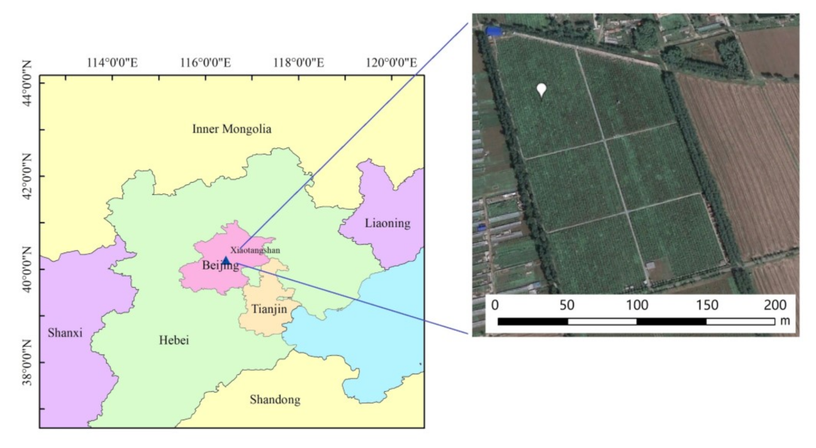
The LAI and corresponding canopy reflectance spectra of 258 samples were measured in the in situ experiments. The experiments were carried out at the China National Experimental Station for Precision Agriculture, located in the town of Xiao Tangshan, Beijing, China (40°11′44′′ N, 116°26′36′′ E, Figure 1). There were 48 plots in 2002 and 22 plots in 2004, and the size of each plot was 32.4 m × 30.0 m. Detail of experiment design can be found in [52]. Canopy reflectance spectra were measured using an ASD FieldSpec Pro spectrometer (Analytical Spectral Devices, Boulder, CO, USA) [53] at a height of 1.3 m above the canopy and under clear sky conditions. The field-of-view angle was 25°, and measurements were carried out between 10:00 and 14:00 local time (see [54] for details). After the spectral measurements, all plants in the 0.6 m × 0.6 m sample area were harvested and transported to the laboratory. Leaves of all the sampled plants were collected together to calculate the LAI. A subsample of leaves was used to determine the leaf area () with an Li-Cor 3100 area meter (Model LI-3100, Li-Cor, Inc., Lincoln, NE, USA) [55]. The LAI for the whole sample area was determined using the following equation (see [52] for details):
2.2. Ancillary Chlleaf Data
The global Chlleaf product, with 300 m resolution in [36], was utilized in the simulation analysis (Section 2.3). This product was generated by the ENVISAT MERIS full resolution surface reflectance product based on the physical model LUT method. The temporal resolution of the product is 7 days, and the time range is from 2003 to early 2012 (Table 1).
Using the 300 m resolution land cover map produced by ENVISAT-MERIS and full resolution data acquired over the year 2005 [56], the mean seasonal phenologies of the vegetation type-specific Chlleaf during 2011 were derived. To evaluate the LAI inversion error caused by the fixed SSA used in the current algorithm when LAI reaches the peak in summer, the maximum values of 8 biomes (Table 2) were selected.
2.3. PROSPECT and 3D-RTM Model Simulations
The leaf optical properties were simulated using the PROSPECT model to derive the empirical relationships between Chlleaf and single scattering albedo (SSA). Leaf reflectance and transmittance are calculated as a function of the chlorophyll content (Chlleaf), carotenoid content (Car), brown matter (Cb), dry matter (Cm), equivalent water (Cw), and leaf structure parameter (N) in the PROSPECT model [58]. The input parameters of the PROSPECT model (Table 3) were set according to the study by Croft et al. [36] and the LOPEX’93 experiment [59].
The canopy reflectance for the 8 biomes in summer was simulated using 3D-RTM model to quantitively compare the accuracy of LAI inverted using the fixed SSA algorithm and Chlleaf-determined dynamic SSA algorithm. Spectral invariant theory simplifies 3D-RTM by decoupling the canopy structure and leaf optics [43]. SSA is the only parameter characterizing the leaf optical property in 3D-RTM parameterization. The average Chlleaf in summer for each biome (recorded in Table 2) was extracted from the global Chlleaf product [36] to derive a more accurate biome-specific SSA. Other key parameters of the 3D-RTM are presented in Table 4.
2.4. LAI Inversions with the Dynamic Leaf Optical Property
The LAI inversion algorithm is based on the biome-specific look-up tables, simulated from the 3D-RTM model. The mean LAI values are calculated from all LAI elements to which the corresponding simulated reflectance in the LUTs are close to red and NIR reflectance within specific uncertainties [21,43]. SSA, which characterizes the leaf optical property in the 3D-RTM model, was set to be fixed values for the 8 biomes in the existing 3D-RTM-based LUT algorithm [41]. To improve the accuracy of leaf optical property in the model inputs, an LAI inversion algorithm based on the Chlleaf-determined SSAred is proposed in this study.
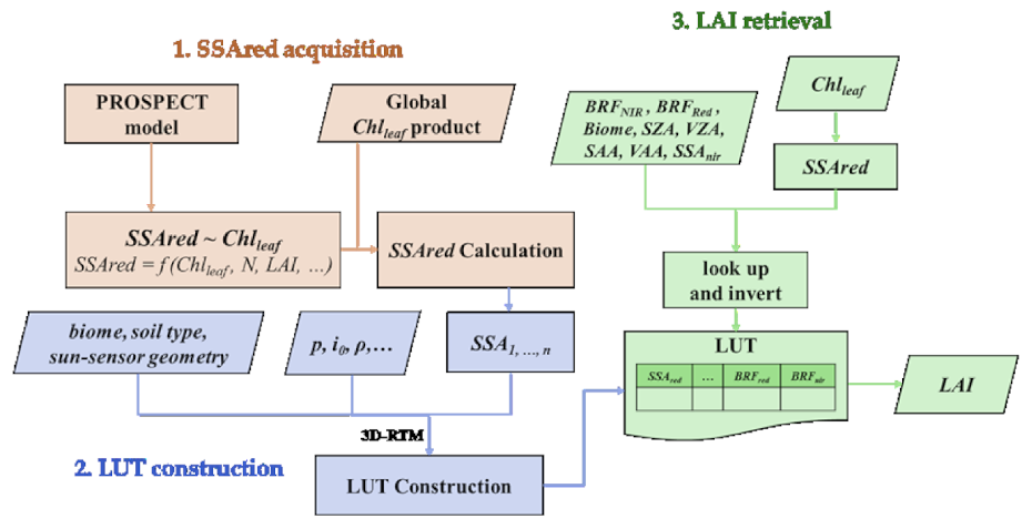
Figure 2 illustrates the diagram of the LAI inversion process with the Chlleaf-determined SSAred. Firstly, SSAred was calculated using the Chlleaf products in step 1. Then, the 3D-RTM was exploited to construct the look-up table. Next, the canopy reflectance, vegetation type, solar-observation geometry, and the corresponding Chlleaf data were used as input parameters to constrain the RTM equations and retrieve the LAI.
2.4.1. Acquisition of Single Scattering Albedo (SSA)
Previous research suggests that there is a strong correlation between the leaf optical properties in the red band and the chlorophyll content [68]. To improve the computational efficiency, the empirical regression models between Chlleaf and SSAred were derived for eight biomes using the PROSPECT model (parameter values given in Table 3). Table 5 describes the biome-specific regression equations between Chlleaf and SSAred. As shown in Table 5, the regression models between SSAred and Chlleaf are of high accuracies, with RMSE ≤ 0.022, and R2 ≥ 0.873. By applying the regression equations to the global Chlleaf product [36], more reasonable SSAred can be calculated.
2.4.2. Construction of LUT Based on the 3D-RTM
Spectral invariant theory effectively simplified the 3D-RTM with three spectral-invariant variables, i.e., re-collision probability (p), canopy interception (i0), and escape probability (ρ), and one spectral-dependent variable—SSA [43]. The spectral invariant parameters of the canopy and the leaf SSA drive the model to reconstruct the radiation field of the canopy [69]. The bidirectional reflectance factors (BRFs) of vegetation canopies can be transformed as follows:
where and are the solar solid angle and observation solid angle, respectively. denotes the wavelength. Other input parameters of 3D-RTM were set as shown in Table 4. Compared with the constant SSA for each biome, SSAred, ranging from 0.05 to 0.25 with an interval of 0.01, were simulated in LUT. SSANIR was still set to be constant since it is irrelevant to leaf chlorophyll content. Then, the look-up table, based on a constant SSA for specific vegetation types, was transformed to the look-up table with a dynamic SSA.
2.4.3. LAI Inversion
The Chlleaf is an additional input variable in LAI inversion apart from the biome, solar-observation geometry (SZA, solar azimuth angle (SAA), VZA, view azimuth angle (VAA)), BRFNIR, and BRFRed. The SSAred value for each pixel was calculated by Chlleaf firstly. SSAred and solar-observation geometry were looked up subsequently, and the items close to the calculated SSAred and the solar-observation geometry of the pixel were selected. Then, the canopy BRFRed and BRFNIR, acquired from satellite images or other observations, were compared with the simulated BRFs of the selected items in LUT as the following function:
BRF and BRF* represent the satellite-derived BRF and simulated BRF in LUT, respectively. σ represents the model and observational uncertainties. If the difference is less than a threshold value ( in this paper), the corresponding LAI in LUT is treated as an acceptable solution. The mean value and the dispersion of these solutions were regarded as the inversed LAI and its uncertainty.
2.4.4. Performance Metrics of the LAI Inversion Algorithm
The performance metrics of the LAI inversion algorithm include the retrieval index (RI), the root mean squared error (RMSE), the coefficient of determination (R2), and the averaged bias (bias). They are defined as follows:
The RI is the percentage of the pixels where the algorithm can find an acceptable solution in the retrieval, which indicates the stability of the algorithm.
RI characterizes the suitability of the algorithm for the given images, but it does not indicate the accuracy. RMSE and R2 are accuracy indicators showing the discrepancy between the retrieved LAI and the reference LAI.
Bias was selected in this study to show the overestimation or the underestimation of the algorithm, as follows:
3. Results
3.1. SSA Calculated from Chlleaf
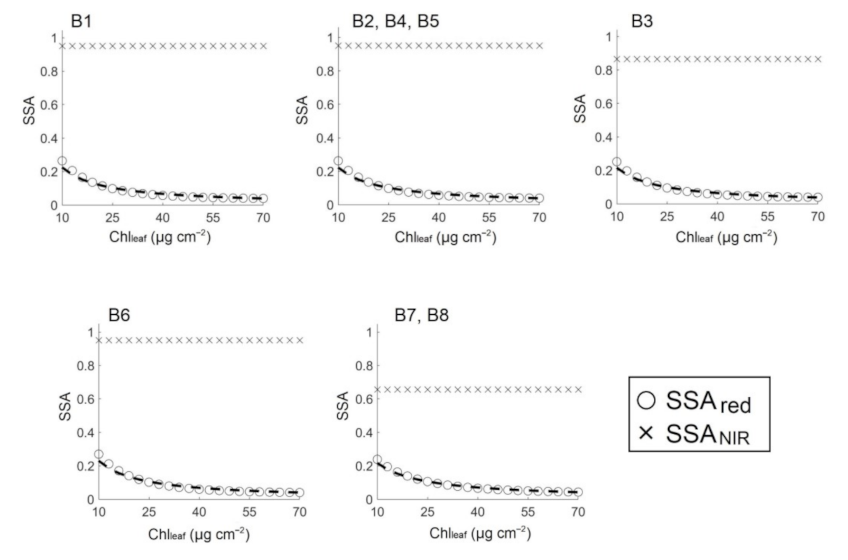
Figure 3 illustrates the PROSPECT-simulated SSA of the 8 biomes in the red (SSAred) and NIR (SSANIR) bands with Chlleaf increasing from 10 to 70 μg cm−2. The SSAred decreased with increasing Chlleaf for all biomes. SSAred dropped from approximately 0.25 to less than 0.15 when Chlleaf increased from 10 to 20 μg cm−2. When Chlleaf increased from 20 to 40 μg cm−2, SSAred declined from less than 0.15 to approximately 0.05. When Chlleaf exceeded 40 μg cm−2, the SSAred remained stable at approximately 0.05. With chlorophyll biosynthesis at the start of a growing season, the absorption of red wavelengths started to increase significantly, leading to a dramatic reduction in the SSAred. When Chlleaf reached the medium to the high level, the absorption became saturated, and the SSAred decreased more slowly. The SSANIR showed insensitivity to Chlleaf and remained constant under all Chlleaf values. However, SSANIR for different biome types varies from 0.65 for evergreen needle forests (B7) and deciduous needle forests (B8) to 0.93 for deciduous broadleaf forests (B6). SSANIR depends more on the leaf internal structure than the pigment content. The differences in the simulated SSANIR for different biomes mainly resulted from the variance in the leaf structure and the dry matter content (Table 3).
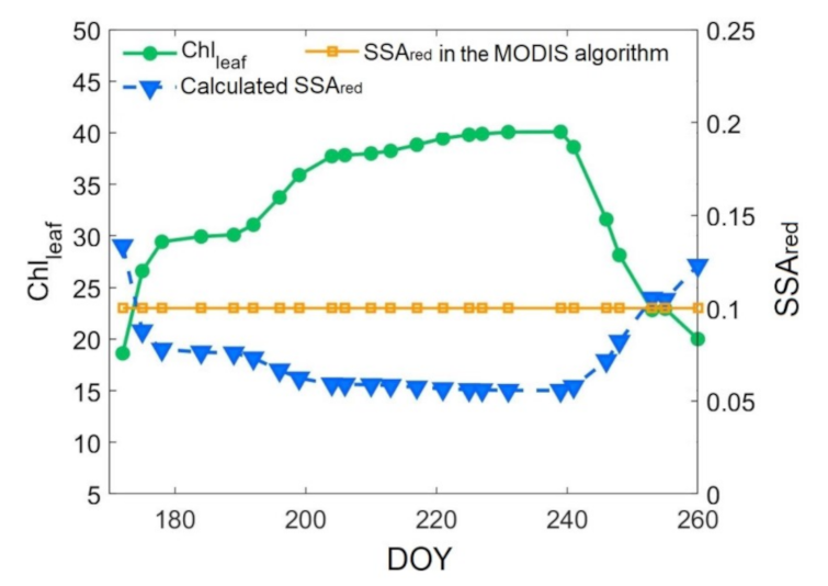
The continuous ground-measured Chlleaf data in one growing season of the soybean samples from the literature [70] and the corresponding SSAred are plotted in Figure 4. Chlleaf showed an expected tendency associated with budburst and chlorophyll biosynthesis after the day of year (DOY) 172, as well as chlorophyll breakdown in autumn (after DOY 239). The SSAred had an inverse tendency with Chlleaf. SSAred exceeded 0.13 before DOY 172 and then decreased sharply by approximately 0.06, reaching 0.078 in the following 6 days, when Chlleaf increased from 18.6 μg cm−2 to 29.4 μg cm−2. Then, SSAred experienced a relatively slow-declining period until DOY 204 (decreased by approximately 0.02 in 26 days), while Chlleaf still increased steadily from 29.4 μg cm−2 to 37.7 μg cm−2. On DOY 204–239, Chlleaf remained stable at 37.7–40.1 μg cm−2, and SSAred remained at 0.05–0.06. From approximately DOY 240, SSAred started to increase and exceeded 0.12, and Chlleaf dropped from 38.6 μg cm−2 to 20.0 μg cm−2. As shown in Figure 4, SSAred changed dramatically from 0.13 to 0.05 during the whole soybean growing season. The fixed SSAred in the current inversion algorithm was usually set to be the average value in the whole growing season for the specific biome type, which overestimated SSAred in the period of high Chlleaf.
3.2. Accuracy of LAI Inversion Using 3D-RTM-Simulated Data
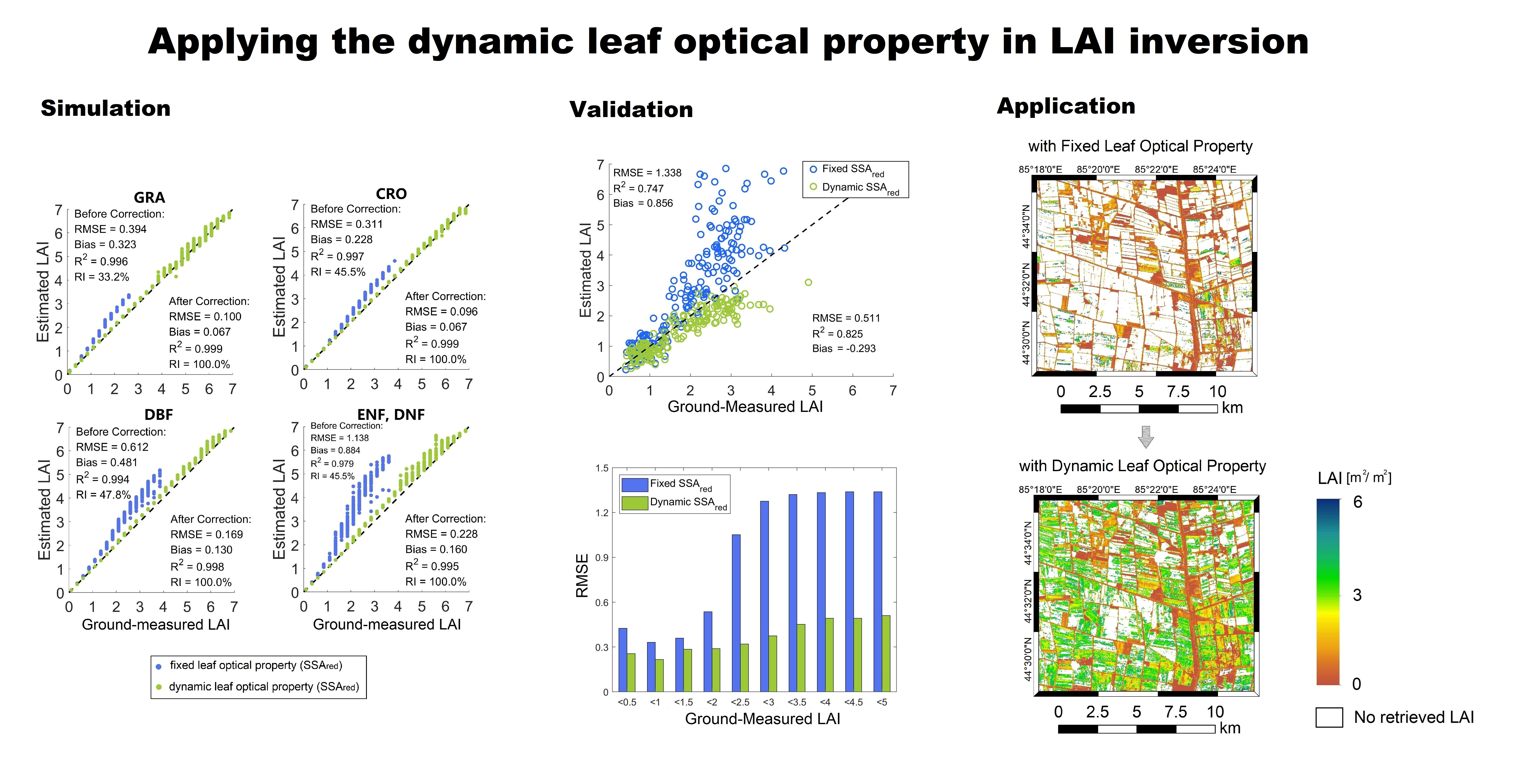
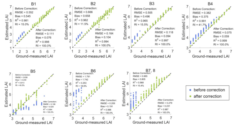
As shown in Figure 4, the difference between the fixed SSAred of the current algorithm and the Chlleaf-determined SSAred was largest when Chlleaf reached the maximum value. There were 1296 simulations of canopy reflectance for each biome with LAI ranging from 1.5 to 6.85 (for B1, 2) or 3 to 6.85 (for B3–8) (other parameters are set as Table 4). Figure 5 and Table 6 compare the LAI inversion results, using the fixed SSAred and the SSAred derived from the analysis of the current Chlleaf product. When Chlleaf was at the peak value in summer, the constant values of SSAred for all 8 biomes are 0.05–0.11 higher than the SSAred determined by the Chlleaf (Table 6). The success rate of the retrieval, with RI ranging from 11.5% (B2: SHR) to 41.7% (B4: SAV), was low. Most-retrieved LAI tended to be overestimated, especially for DBF(B6) and NF(B7, 8) with bias of 1.742 and 0.805, respectively. EBF(B5) had underestimation with RMSE of 0.638 and bias of −0.230. The algorithm with the Chlleaf-determined SSAred had a higher inversion rate and accuracy. RI increased to 100% for all 8 biomes (Figure 5). RMSE decreased from 0.382–1.791 to no more than 0.279 for different biomes, and the bias decreased to less than 0.231.
Figure 6 illustrates the accuracy of LAI inversion in one growing season using the 3D-RTM simulated reflectance. The leaf chlorophyll content was set as the ground-measured values, as shown in Figure 4. RMSE of the retrieved LAI using the fixed SSAred algorithm was larger at the start and end of the growing season (Figure 6a). With the increasing of Chlleaf, RMSE dropped dramatically and remained stable at approximately 0.5 during DOY 204–241. RI decreased dramatically to 52.8%–56.0% on DOY 204 and DOY 241 (Figure 6b), and previous research proved the algorithm tended to fail more often in the summer period [71]. The Chlleaf-determined SSAred algorithm showed higher accuracy (RMSE < 0.1) and stability (RI = 100%) in the whole growing season.
3.3. Validation with Ground Measurements
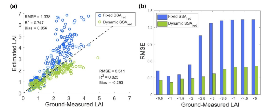
Figure 7a validated the LAI inversion using the ground-measured data from the Xiao Tangshan site. The LAI retrieved by the 3D-RTM model with the fixed SSAred (0.18 for cereal crops), as in the MODIS LAI product algorithm [21], had a significant overestimation with RMSE of 1.338, bias of 0.856, and R2 of 0.747. The dynamic SSAred algorithm performed better with RMSE of 0.511 and R2 of 0.825. When LAI was higher than 2, the RMSE of the fixed SSAred algorithm increased to 1.786, which indicated that large inversion error occurred under high LAI and high Chlleaf values. RMSE of the dynamic SSAred algorithm was 0.513 when LAI was larger than 2, which was nearly the same as the overall RMSE (0.511). Figure 7b illustrated the average RMSE with an LAI interval of 0.5. It also shows the high inversion error under large LAI and Chlleaf conditions for the fixed SSAred algorithm. The accuracy of the dynamic SSAred algorithm was relatively stable for different LAI values with RMSE less than 0.6.
4. Discussion
The LAI inversion accuracy was significantly improved by introducing the dynamic SSA to the 3D-RTM-based inversion algorithm, especially in summer, for high Chlleaf values (Figure 5, Figure 6 and Figure 7 and Table 6). Overestimations of the existing 3D-RTM-based LUT method algorithm under high LAI conditions have been recorded in many studies and analyses [72,73,74]. One reason is the high setting of SSAred in the existing algorithm. SSAred, defined as the leaf reflectance plus leaf transmittance, is an indicator of the leaf scattering ability. The SSA was actually influenced by the leaf internal structure of tissues and leaf biochemical composition [58]. In the existing algorithm, the SSA was determined by the sensor-specific resolution and spectral band setup [10]. The algorithm needs to adjust SSA to apply in other sensors [23,42]. The fixed values of SSA were always close to the average value over the whole growing season to guarantee the overall accuracy and stability. However, the fixed value of the SSAred is higher than the actual SSAred in summer (Figure 4) [59,75], which suggests a larger proportion of light scattering out of leaves in the single interaction between photons and leaves. A larger scattering proportion means less absorption of leaf chlorophyll, which leads to a high simulation of BRFRed in the look-up table. The input BRFRed under the same canopy condition has to look up the low reflectance with a larger LAI and more absorption in the red band. The inversion scheme finally produced a higher LAI inversion result [76]. Likewise, at the start and end of the growing season, when the fixed SSAred was lower than the actual value, the retrieved LAI tended to be underestimated [77]. Thus, the dynamic SSAred algorithm proposed in this study provides a practical way to avoid these problems and enhance accuracy. In this study, the accuracy improvement on the croplands was validated using the ground-measured data. Future work can make further validation and evaluation on other vegetation types.
The dynamic SSA algorithm also increases the retrieval index (RI), which suggests the robustness of the algorithm (Table 6, Figure 6b). If all the BRF values simulated in the LUT fail to match the input BRF, the inversion failure appears. Previous studies suggested the algorithm failure frequently occurred in tropical areas or summer periods using the fixed SSAred [71,78]. The potential reason may be that the fixed SSAred algorithm tended to overestimate the SSAred and subsequently retrieve an overestimated LAI when the LAI was less than 4 (Figure 5 and Figure 7a). For higher LAI, even the highest LAI in the LUT cannot simulate values as low as the input BRFRed. Therefore, the inversion process by the algorithm fails, as shown in Table 6 and Figure 6b. The proposed algorithm simulated the radiation transfer process within the canopy more precisely through the dynamic SSAred closer to the actual scenarios, which makes the simulated reflectance more consistent with the actual reflectance of pixels. More accurate solutions were determined during the inversion process.
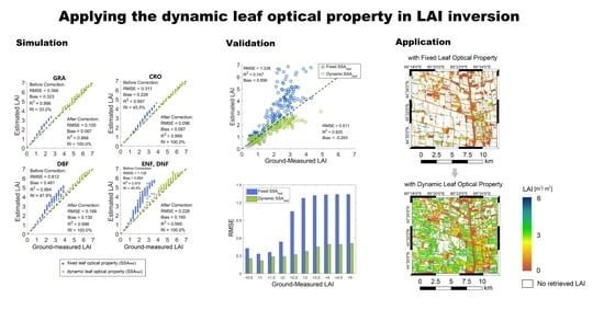
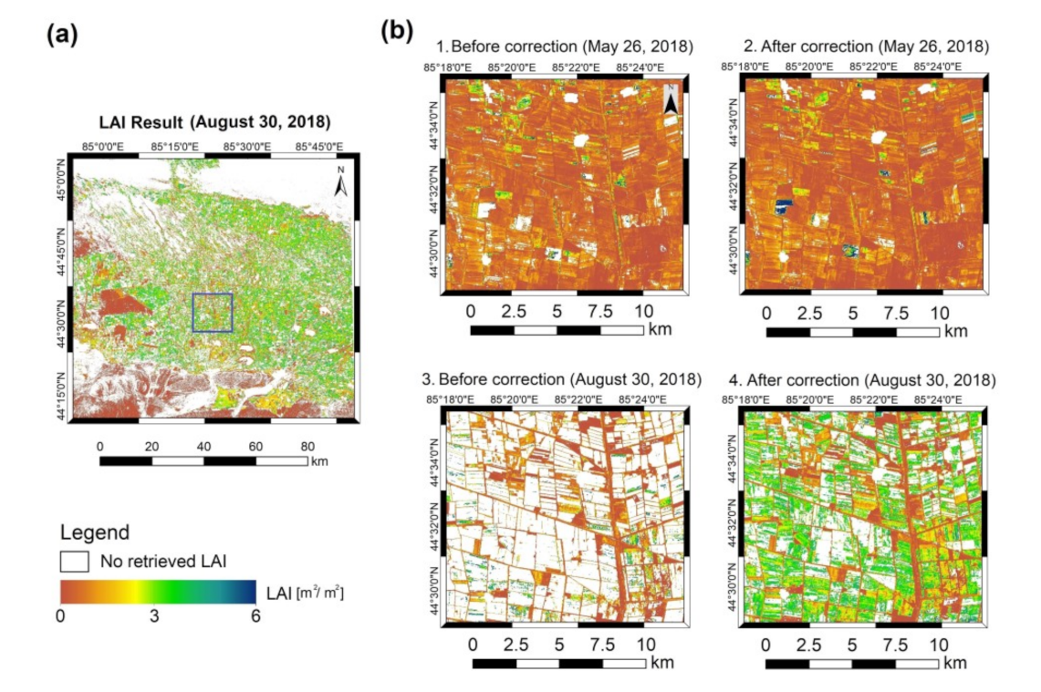
The algorithm proposed in this study has the potential to be applied to satellite images. The following figure (Figure 8) demonstrated the LAI results inversed from the Sentinel-2 images with the proposed algorithm. The Chlleaf product, over the same period in the area, was calculated using the Chlorophyll Sensitive Index (CSI) regression method proposed in [51]. At the start of the season on May 26, 2018, the LAI retrieved by the fixed SSAred algorithm and the dynamic SSAred algorithm is close. The fixed SSAred is close to the Chlleaf-determined SSAred. At the peak of LAI on August 30, 2018, the proposed algorithm has significantly higher RI than the fixed SSAred algorithm, which indicates that the proposed algorithm simulated the canopy radiative transfer process more precisely, through the SSAred, which was closer to the actual scenarios. The fixed parameterizations of the leaf optical properties in the algorithm were decided by the background, indicating that no global Chlleaf product or well-performed Chlleaf inversion methods were available at that time. At present, more Chlleaf products are becoming available and extensively validated, which makes the algorithm considering the leaf optical properties in the radiative transfer model applicable.
The errors of leaf chlorophyll content product (e.g., the RMSE of the Chlleaf product used in this study is 10.8 μg cm−2) [36] will bring uncertainties to the estimation of SSAred and further LAI inversion. To balance the uncertainty of the Chlleaf product and the information gain in applying to the satellite data, the SSAred can be set to several discrete values in the whole growing season, such as for the start of the growing season, for the high-LAI conditions in summer, and the senescence period. Apart from the Chlleaf, there are still many assumptions regarding the pixel scenario and predetermined values of the biophysical parameters in the present algorithm, such as soil optical properties, which deviate from the actual situation. Dynamic values, which are close to the actual situation, are needed to improve the LAI inversion accuracy. For example, the optical properties of NIR correlate closely with the leaf dry matter content [79,80] and in the shortwave infrared (SWIR) bands with the leaf water content and leaf internal structure [81]. In the future, if more precise information of these variables can be used in the inversion, a more accurate LAI can be acquired.
5. Conclusions
In this paper, an LAI inversion algorithm was proposed by considering the leaf optical properties in 3D-RTM. The algorithm calculated the SSA using the leaf chlorophyll content and extended the 3D-RTM-based look-up table by adding an SSAred item. The Chlleaf-determined SSAred changed dramatically with the leaf biochemistry concentration in a growing season, which is closer to the actual scenarios, compared with the fixed SSA algorithm. Thus, the accuracy of the retrieved LAI and the stability of the algorithm improved with the dynamic SSAred. The analysis with simulated data showed that RMSE decreased from 0.382–1.971 of the fixed SSAred algorithm to less than 0.075–0.279 of the proposed algorithm for eight biomes, and the retrieval index increased from ≤41.7% to 100%. The validation with the ground measurements also showed the improvement. RMSE decreased from 1.338 to 0.511, and the accuracy kept stable under different LAI values. The proposed algorithm also weakens the overestimation and high inversion failure rate under high LAI values. The precise calculation of leaf optical properties improves the model-based LAI inversion. However, the application of the proposed algorithm in LAI product generation needs the accurate Chlleaf product or further research on prior knowledge derivation, based on the present Chlleaf product.
Author Contributions
Data curation, Z.Z. and L.L.; Formal analysis, H.Z.; Funding acquisition, J.L. and Q.L.; Methodology, H.Z.; Project administration, Q.L.; Resources, L.L.; Software, S.L. and Z.Z.; Supervision, Q.L.; Validation, J.Z.; Visualization, Xinran Zhu; Writing – original draft, H.Z.; Writing – review & editing, J.L. and Y.D. All authors have read and agreed to the published version of the manuscript.
Funding
This research was supported by the National Key Research and Development Program of China (2017YFA0603001), GF6 Project under Grant 30-Y20A03-9003-17/18, and National Natural Science Foundation of China (No. 41671374).
Acknowledgments
Thanks are due to Ranga B. Myneni and Yuri Knyazikhin for assistance with the valuable discussion. We also appreciate the Center for Advanced Land Management Information Technologies (CALMIT), University of Nebraska–Lincoln, for providing us with the in situ spectra and biochemical datasets for the US-Ne2 and US-Ne3 sites.
Conflicts of Interest
The authors declare no conflict of interest.
References
- Chen, J.M.; Black, T.A. Defining leaf area index for non-flat leaves. Plant Cell Environ. 1992, 15, 421–429. [Google Scholar] [CrossRef]
- Myneni, R.B.; Hoffman, S.; Knyazikhin, Y.; Privette, J.L.; Glassy, J.; Tian, Y.; Wang, Y.; Song, X.; Zhang, Y.; Smith, G.R.; et al. Global products of vegetation leaf area and fraction absorbed PAR from year one of MODIS data. Remote Sens. Environ. 2002, 83, 214–231. [Google Scholar] [CrossRef] [Green Version]
- Alton, P.B. The sensitivity of models of gross primary productivity to meteorological and leaf area forcing: A comparison between a Penman–Monteith ecophysiological approach and the MODIS Light-Use Efficiency algorithm. Agric. For. Meteorol. 2016, 218, 11–24. [Google Scholar] [CrossRef] [Green Version]
- Asner, G.P.; Braswell, B.H.; Schimel, D.S.; Wessman, C.A. Ecological Research Needs from Multiangle Remote Sensing Data. Remote Sens. Environ. 1998, 63, 155–165. [Google Scholar] [CrossRef]
- Boussetta, S.; Balsamo, G.; Beljaars, A.; Kral, T.; Jarlan, L. Impact of a satellite-derived leaf area index monthly climatology in a global numerical weather prediction model. Int. J. Remote Sens. 2013, 34, 3520–3542. [Google Scholar] [CrossRef]
- Jarlan, L.; Balsamo, G.; Lafont, S.; Beljaars, A.; Calvet, J.C.; Mougin, E. Analysis of leaf area index in the ECMWF land surface model and impact on latent heat and carbon fluxes: Application to West Africa. J. Geophys. Res. Atmos. 2008, 2008, 113. [Google Scholar] [CrossRef]
- Fang, H.; Zhang, Y.; Wei, S.; Li, W.; Ye, Y.; Sun, T.; Liu, W. Validation of global moderate resolution leaf area index (LAI) products over croplands in northeastern China. Remote Sens. Environ. 2019, 233, 111377. [Google Scholar] [CrossRef]
- Gonsamo, A.; Chen, J.M. Improved LAI Algorithm Implementation to MODIS Data by Incorporating Background, Topography, and Foliage Clumping Information. IEEE Trans. Geosci. Remote Sens. 2014, 52, 1076–1088. [Google Scholar] [CrossRef]
- Knyazikhin, Y.; Martonchik, J.V.; Diner, D.J.; Myneni, R.B.; Verstraete, M.; Pinty, B.; Gobron, N. Estimation of vegetation canopy leaf area index and fraction of absorbed photosynthetically active radiation from atmosphere-corrected MISR data. J. Geophys. Res. Atmos. 1998, 103, 32239–32256. [Google Scholar] [CrossRef] [Green Version]
- Yan, K.; Park, T.; Chen, C.; Xu, B.; Song, W.; Yang, B.; Zeng, Y.; Liu, Z.; Yan, G.; Knyazikhin, Y.; et al. Generating Global Products of LAI and FPAR From SNPP-VIIRS Data: Theoretical Background and Implementation. IEEE Trans. Geosci. Remote Sens. 2018, 56, 2119–2137. [Google Scholar] [CrossRef]
- Tum, M.; Günther, K.P.; Böttcher, M.; Baret, F.; Bittner, M.; Brockmann, C.; Weiss, M. Global Gap-Free MERIS LAI Time Series (2002–2012). Remote Sens. 2016, 8, 69. [Google Scholar] [CrossRef] [Green Version]
- Baret, F.; Weiss, M.; Lacaze, R.; Camacho, F.; Makhmara, H.; Pacholcyzk, P.; Smets, B. GEOV1: LAI and FAPAR essential climate variables and FCOVER global time series capitalizing over existing products. Part1: Principles of development and production. Remote Sens. Environ. 2013, 137, 299–309. [Google Scholar] [CrossRef]
- Xiao, Z.; Liang, S.; Wang, J.; Chen, P. Use of General Regression Neural Networks for Generating the GLASS Leaf Area Index Product From Time-Series MODIS Surface Reflectance. IEEE Trans. Geosci. Remote Sens. 2014, 52, 209–223. [Google Scholar] [CrossRef]
- Deng, F.; Chen, J.; Plummer, S.; Chen, M.; Pisek, J. Algorithm for global leaf area index retrieval using satellite imagery. IEEE Trans. Geosci. Remote Sens. 2006, 44, 2219–2229. [Google Scholar] [CrossRef] [Green Version]
- Colombo, R.; Bellingeri, D.; Fasolini, D.; Marino, C.M. Retrieval of leaf area index in different vegetation types using high resolution satellite data. Remote Sens. Environ. 2003, 86, 120–131. [Google Scholar] [CrossRef]
- Meroni, M.; Colombo, R.; Panigada, C. Inversion of a radiative transfer model with hyperspectral observations for LAI mapping in poplar plantations. Remote Sens. Environ. 2004, 92, 195–206. [Google Scholar] [CrossRef]
- Huang, D.; Knyazikhin, Y.; Wang, W.; Deering, D.W.; Stenberg, P.; Shabanov, N.; Tan, B.; Myneni, R.B. Stochastic transport theory for investigating the three-dimensional canopy structure from space measurements. Remote Sens. Environ. 2008, 112, 35–50. [Google Scholar] [CrossRef]
- Camacho, F.; Cernicharo, J.; Lacaze, R.; Baret, F.; Weiss, M. GEOV1: LAI, FAPAR essential climate variables and FCOVER global time series capitalizing over existing products. Part 2: Validation and intercomparison with reference products. Remote Sens. Environ. 2013, 137, 310–329. [Google Scholar] [CrossRef]
- Baret, F.; Hagolle, O.; Geiger, B.; Bicheron, P.; Miras, B.; Huc, M.; Berthelot, B.; Niño, F.; Weiss, M.; Samain, O.; et al. LAI, fAPAR and fCover CYCLOPES global products derived from VEGETATION: Part 1: Principles of the algorithm. Remote Sens. Environ. 2007, 110, 275–286. [Google Scholar] [CrossRef] [Green Version]
- Jacquemoud, S.; Verhoef, W.; Baret, F.; Bacour, C.; Zarco-Tejada, P.J.; Asner, G.P.; François, C.; Ustin, S.L. PROSPECT+SAIL models: A review of use for vegetation characterization. Remote Sens. Environ. 2009, 113, S56–S66. [Google Scholar] [CrossRef]
- Knyazikhin, Y.; Glassy, J.; Privette, J.L.; Tian, Y.; Lotsch, A.; Zhang, Y.; Wang, Y.; Morisette, J.T.; Votava, P.; Myneni, R.B.; et al. MODIS Leaf Area Index (LAI) and Fraction of Photosynthetically Active Radiation Absorbed by Vegetation (FPAR) Product (MOD15) Algorithm Theoretical Basis Document. 1999. Available online: http://eospso.gsfc.nasa.gov/atbd/modistables.html (accessed on 2 December 2021).
- Fang, H.; Baret, F.; Plummer, S.; Schaepman-Strub, G. An Overview of Global Leaf Area Index (LAI): Methods, Products, Validation, and Applications. Rev. Geophys. 2019, 57, 739–799. [Google Scholar] [CrossRef]
- Xu, B.; Park, T.; Yan, K.; Chen, C.; Zeng, Y.; Song, W.; Yin, G.; Li, J.; Liu, Q.; Knyazikhin, Y.; et al. Analysis of Global LAI/FPAR Products from VIIRS and MODIS Sensors for Spatio-Temporal Consistency and Uncertainty from 2012–2016. Forests 2018, 9, 73. [Google Scholar] [CrossRef] [Green Version]
- GCOS. The Global Observing System for Climate: Implementation Needs (GCOS-200). 2016. Available online: https://library.wmo.int/opac/doc_num.php?explnum_id=3417 (accessed on 2 December 2021).
- Combal, B.; Baret, F.; Weiss, M.; Trubuil, A.; Macé, D.; Pragnère, A.; Myneni, R.; Knyazikhin, Y.; Wang, L. Retrieval of canopy biophysical variables from bidirectional reflectance using prior information to solve the ill-posed inverse problem. Remote Sens. Environ. 2003, 84, 1–15. [Google Scholar] [CrossRef]
- Weiss, M.; Baret, F. Evaluation of Canopy Biophysical Variable Retrieval Performances from the Accumulation of Large Swath Satellite Data. Remote Sens. Environ. 1999, 70, 293–306. [Google Scholar] [CrossRef]
- Combal, B.; Baret, F.; Weiss, M. Improving canopy variables estimation from remote sensing data by exploiting ancillary information. Case study on sugar beet canopies. Agronomie 2002, 22, 205–215. [Google Scholar] [CrossRef]
- Zhu, X.; Feng, X.; Zhao, Y. Multi-scale MSDT inversion based on LAI spatial knowledge. Sci. China Earth Sci. 2012, 55, 1297–1305. [Google Scholar] [CrossRef]
- Quan, X.; He, B.; Li, X. A Bayesian Network-Based Method to Alleviate the Ill-Posed Inverse Problem: A Case Study on Leaf Area Index and Canopy Water Content Retrieval. IEEE Trans. Geosci. Remote Sens. 2015, 53, 6507–6517. [Google Scholar] [CrossRef]
- Shiklomanov, A.; Bradley, B.; Dahlin, K.; Fox, A.; Gough, C.; Hoffman, F.; Middleton, E.; Serbin, S.; Smallman, T.; Smith, W. Enhancing global change experiments through integration of remote-sensing techniques. Front. Ecol. Environ. 2019, 17, 215–224. [Google Scholar] [CrossRef] [Green Version]
- Wu, S.; Zeng, Y.; Hao, D.; Liu, Q.; Li, J.; Chen, X.; Asrar, G.R.; Yin, G.; Wen, J.; Yang, B.; et al. Quantifying leaf optical properties with spectral invariants theory. Remote Sens. Environ. 2021, 253, 112131. [Google Scholar] [CrossRef]
- Yi, Y.; Yang, D.; Huang, J.; Chen, D. Evaluation of MODIS surface reflectance products for wheat leaf area index (LAI) retrieval. Isprs J. Photogramm. Remote Sens. 2008, 63, 661–677. [Google Scholar] [CrossRef]
- Sims, D.A.; Gamon, J.A. Relationships between leaf pigment content and spectral reflectance across a wide range of species, leaf structures and developmental stages. Remote Sens. Environ. 2002, 81, 337–354. [Google Scholar] [CrossRef]
- Croft, H.; Chen, J.M.; Zhang, Y. Temporal disparity in leaf chlorophyll content and leaf area index across a growing season in a temperate deciduous forest. Int. J. Appl. Earth Obs. Geoinf. 2014, 33, 312–320. [Google Scholar] [CrossRef]
- Demarez, V. Seasonal variation of leaf chlorophyll content of a temperate forest. Inversion of the PROSPECT model. Int. J. Remote Sens. 1999, 20, 879–894. [Google Scholar] [CrossRef]
- Croft, H.; Chen, J.M.; Wang, R.; Mo, G.; Luo, S.; Luo, X.; He, L.; Gonsamo, A.; Arabian, J.; Zhang, Y.; et al. The global distribution of leaf chlorophyll content. Remote Sens. Environ. 2020, 236. [Google Scholar] [CrossRef]
- Gitelson, A.A.; Merzlyak, M.N. Signature Analysis of Leaf Reflectance Spectra: Algorithm Development for Remote Sensing of Chlorophyll. J. Plant Physiol. 1996, 148, 494–500. [Google Scholar] [CrossRef]
- Xu, X. Remote Sensing Physics; Peking University Press: Beijing, China, 2005. (In Chinese) [Google Scholar]
- Blackburn, G.A. Relationships between Spectral Reflectance and Pigment Concentrations in Stacks of Deciduous Broadleaves. Remote Sens. Environ. 1999, 70, 224–237. [Google Scholar] [CrossRef]
- Liu, J.; Li, J.; Liu, Q.; He, B.; Yu, W. Global Leaf Spectral Characteristics of Typical Vegetation and It’s Impacts on LAI Inversion. Remote Sens. Technol. Appl. (In Chinese). 2019, 34, 155–165. [Google Scholar]
- Park, T.; Yan, K.; Chen, C.; Xu, B.; Knyazikhin, Y.; Myneni, R. VIIRS Leaf Area Index (LAI) and Fraction of Photosynthetically Active Radiation Absorbed by Vegetation (FPAR) Product Algorithm Theoretical Basis Document (ATBD). 2018. Available online: https://lpdaac.usgs.gov/documents/125/VNP15_ATBD.pdf (accessed on 2 December 2021).
- Ganguly, S.; Nemani, R.R.; Zhang, G. Generating global Leaf Area Index from Landsat: Algorithm formulation and demonstration. Remote Sens. Environ. 2012, 122, 185–202. [Google Scholar] [CrossRef] [Green Version]
- Knyazikhin, Y.; Martonchik, J.V.; Myneni, R.B.; Diner, D.J.; Running, S.W. Synergistic algorithm for estimating vegetation canopy leaf area index and fraction of absorbed photosynthetically active radiation from MODIS and MISR data. J. Geophys. Res. Atmos. 1998, 103, 32257–32275. [Google Scholar] [CrossRef] [Green Version]
- Horler, D.N.H.; Dockray, M.; Barber, J. The red edge of plant leaf reflectance. Int. J. Remote Sens. 1983, 4, 273–288. [Google Scholar] [CrossRef]
- Lemaire, G.; Francois, C.; Soudani, K.; Berveiller, D.; Pontailler, J.; Breda, N.; Genet, H.; Davi, H.; Dufrene, E. Calibration and validation of hyperspectral indices for the estimation of broadleaved forest leaf chlorophyll content, leaf mass per area, leaf area index and leaf canopy biomass. Remote Sens. Environ. 2008, 112, 3846–3864. [Google Scholar] [CrossRef]
- Zarco-Tejada, P.J.; Hornero, A.; Beck, P.S.A.; Kattenborn, T.; Kempeneers, P.; Hernandez-Clemente, R. Chlorophyll content estimation in an open-canopy conifer forest with Sentinel-2A and hyperspectral imagery in the context of forest decline. Remote Sens. Environ. 2019, 223, 320–335. [Google Scholar] [CrossRef] [PubMed]
- Croft, H.; Chen, J.M.; Zhang, Y.; Simic, A. Modelling leaf chlorophyll content in broadleaf and needle leaf canopies from ground, CASI, Landsat TM 5 and MERIS reflectance data. Remote Sens. Environ. 2013, 133, 128–140. [Google Scholar] [CrossRef]
- Verrelst, J.; Mu?oz, J.; Alonso, L.; Delegido, J.; Rivera, J.P.; Camps-Valls, G.; Moreno, J. Machine learning regression algorithms for biophysical parameter retrieval: Opportunities for Sentinel-2 and -3. Remote Sens. Environ. 2012, 118, 127–139. [Google Scholar] [CrossRef]
- Xu, M.; Liu, R.; Chen, J.M.; Liu, Y.; Shang, R.; Ju, W.; Wu, C.; Huang, W. Retrieving leaf chlorophyll content using a matrix-based vegetation index combination approach. Remote Sens. Environ. 2019, 224, 60–73. [Google Scholar] [CrossRef]
- Li, J.; Zhang, H.; Wang, X.; Zhang, Z.; Gu, C.; Wen, Y.; Chu, T.; Liu, Q. MuSyQ 30m/10days Leaf Chlorophyll Content Product (From 2019 to 2020 across China Version 01); Science Data Bank: Beijing, China, 2021. [Google Scholar] [CrossRef]
- Zhang, H.; Li, J.; Liu, Q.; Zhao, J.; Dong, Y. A highly chlorophyll-sensitive and LAI-insensitive index based on the red-edge band: CSI. In Proceedings of the IGARSS 2020—2020 IEEE International Geoscience and Remote Sensing Symposium, Waikoloa, HI, USA, 26 September–2 October 2020. [Google Scholar]
- Huang, W.J.; Niu, Z.; Wang, J.H.; Liu, L.Y.; Zhao, C.J.; Liu, Q. Identifying crop leaf angle distribution based on two-temporal and bidirectional canopy reflectance. IEEE Trans. Geosci. Remote Sens. 2006, 44, 3601–3609. [Google Scholar] [CrossRef]
- Hatchell, D.C. (ASD) Technical Guide; Analytical Spectral Devices Inc.: Boulder, CO, USA, 1999; p. 136. [Google Scholar]
- Liu, L.; Wang, J.; Huang, W.; Zhao, C. Detection of leaf and canopy EWT by calculating REWT from reflectance spectra. Int. J. Remote Sens. 2010, 31, 2681–2695. [Google Scholar] [CrossRef]
- LI-3100 Area Meter Instruction Manual; LI-COR: Lincoln, NE, USA, 1996. Available online: https://www.licor.com/documents/mic5csqh1d11skf7n1uo (accessed on 2 December 2021).
- Bicheron, P.; Leroy, M.; Brockmann, C.; Krämer, U.; Miras, B.; Huc, M.; Niño, F.; Defourny, P.; Vancutsem, C.; Arino, O.; et al. Globcover: A 300 m global land cover product for 2005 using ENVISAT MERIS time series. In Proceedings of the Second International Symposium on Recent Advances in Quantitative Remote Sensing 2006, Enschede, The Netherlands, 8–11 May 2006; 2006; pp. 538–542. Available online: http://citeseerx.ist.psu.edu/viewdoc/download?doi=10.1.1.116.1909&rep=rep1&type=pdf (accessed on 2 December 2021).
- Friedl, M.; Sulla-Menashe, D. MCD12Q1 MODIS/Terra+Aqua Land Cover Type Yearly L3 Global 500 m SIN Grid V006; Distributed by NASA EOSDIS Land Processes DAAC. 2019. Available online: https://lpdaac.usgs.gov/products/mcd12q1v006/ (accessed on 2 December 2021).
- Jacquemoud, S.; Baret, F. PROSPECT: A model of leaf optical properties spectra. Remote Sens. Environ. 1990, 34, 75–91. [Google Scholar] [CrossRef]
- Hosgood, B.; Jacquemoud, S.; Andreoli, G.; Verdebout, J.; Pedrini, G.; Schmuck, G. Leaf Optical Properties EXperiment 93 (LOPEX93); Report EUR 16095 EN; European Commission, Joint Research Centre, Institute for Remote Sensing Applications: Brussels, Belgium, 1994; Available online: https://data.ecosis.org/dataset/13aef0ce-dd6f-4b35-91d9-28932e506c41/resource/4029b5d3-2b84-46e3-8fd8-c801d86cf6f1/download/leaf-optical-properties-experiment-93-lopex93.pdf (accessed on 2 December 2021).
- Darvishzadeh, R.; Skidmore, A.; Schler, F.M.; Atzberger, C. Inversion of a radiative transfer model for estimating vegetation LAI and chlorophyll in a heterogeneous grassland. Remote Sens. Environ. 2008, 112, 2592–2604. [Google Scholar] [CrossRef]
- Enrique, G.D.d.l.R.; Manuel, O.; Hendrik, P.; Luis, U.J.; Rafael, V.; Cristina, A. Leaf Mass per Area (LMA) and Its Relationship with Leaf Structure and Anatomy in 34 Mediterranean Woody Species along a Water Availability Gradient. PLoS ONE 2016, 11, e0148788. [Google Scholar]
- Momadou, S.; Cheikh, M.; Christelle, H.; Rasmus, F.; Bienvenu, S. Estimation of Herbaceous Fuel Moisture Content Using Vegetation Indices and Land Surface Temperature from MODIS Data. Remote Sens. 2013, 5, 2617–2638. [Google Scholar]
- Jacquemoud, S.; Bacour, C.; Poilvé, H.; Frangi, J.P. Comparison of Four Radiative Transfer Models to Simulate Plant Canopies Reflectance: Direct and Inverse Mode. Remote Sens. Environ. 2000, 74, 471–481. [Google Scholar] [CrossRef]
- Arellano, P.; Tansey, K.; Balzter, H.; Boyd, D.S. Field spectroscopy and radiative transfer modelling to assess impacts of petroleum pollution on biophysical and biochemical parameters of the Amazon rainforest. Environ. Earth Sci. 2017, 76, 217. [Google Scholar] [CrossRef] [Green Version]
- Féret, J.-B.; Franois, C.; Gitelson, A.; Asner, G.P.; Barry, K.M.; Panigada, C.; Richardson, A.D.; Jacquemoud, S. Optimizing spectral indices and chemometric analysis of leaf chemical properties using radiative transfer modeling—ScienceDirect. Remote Sens. Environ. 2011, 115, 2742–2750. [Google Scholar] [CrossRef] [Green Version]
- Koetz, B.; Schaepman, M.E.; Morsdorf, F.; Bowyer, P.; Itten, K.I.; Allgöwer, B. Radiative transfer modeling within a heterogeneous canopy for estimation of forest fire fuel properties. Remote Sens. Environ. 2004, 92, 332–344. [Google Scholar] [CrossRef]
- De Santis, A.; Chuvieco, E.; Vaughan, P.J. Short-term assessment of burn severity using the inversion of PROSPECT and GeoSail models. Remote Sens. Environ. 2009, 113, 126–136. [Google Scholar] [CrossRef]
- Thomas, J.R.; Gausman, H.W. Leaf Reflectance vs. Leaf Chlorophyll and Carotenoid Concentrations for Eight Crops. Agron. J. 1977, 69, 799–802. [Google Scholar] [CrossRef]
- Wang, Y.; Buermann, W.; Stenberg, P.; Smolander, H.; Häme, T.; Tian, Y.; Hu, J.; Knyazikhin, Y.; Myneni, R.B. A new parameterization of canopy spectral response to incident solar radiation: Case study with hyperspectral data from pine dominant forest. Remote Sens. Environ. 2003, 85, 304–315. [Google Scholar] [CrossRef]
- Gitelson, A.A. Remote estimation of canopy chlorophyll content in crops. Geophys. Res. Lett. 2005, 32, 8. [Google Scholar] [CrossRef] [Green Version]
- Tan, B.; Hu, J.; Dong, H.; Yang, W.; Zhang, P.; Shabanov, N.V.; Knyazikhin, Y.; Nemani, R.R.; Myneni, R.B. Assessment of the broadleaf crops leaf area index product from the Terra MODIS instrument. Agric. For. Meteorol. 2006, 135, 124–134. [Google Scholar] [CrossRef]
- Yang, W.; Tan, B.; Huang, D.; Rautiainen, M.; Shabanov, N.V.; Wang, Y.; Privette, J.L.; Huemmrich, K.F.; Fensholt, R.; Sandholt, I. MODIS leaf area index products: From validation to algorithm improvement. IEEE Trans. Geosci. Remote Sens. 2006, 44, 1885–1898. [Google Scholar] [CrossRef]
- Hill, M.J.; Senarath, U.; Lee, A.; Zeppel, M.; Nightingale, J.M.; Williams, R.J.; McVicar, T.R. Assessment of the MODIS LAI product for Australian ecosystems. Remote Sens. Environ. 2006, 101, 495–518. [Google Scholar] [CrossRef]
- Jensen, J.; Humes, K.S.; Hudak, A.T.; Vierling, L.A.; Delmelle, E. Evaluation of the MODIS LAI product using independent lidar-derived LAI: A case study in mixed conifer forest. Remote Sens. Environ. 2011, 115, 3625–3639. [Google Scholar] [CrossRef] [Green Version]
- Mottus, M.; Rautiainen, M. Direct retrieval of the shape of leaf spectral albedo from multiangular hyperspectral Earth observation data. Remote Sens. Environ. 2009, 113, 1799–1807. [Google Scholar] [CrossRef]
- Serbin, S.P.; Ahl, D.E.; Gower, S.T. Spatial and temporal validation of the MODIS LAI and FPAR products across a boreal forest wildfire chronosequence. Remote Sens. Environ. 2013, 133, 71–84. [Google Scholar] [CrossRef]
- Zhang, W.; Chen, Y.; Hu, S. Retrieving LAI in the Heihe and the Hanjiang river basins using landsat images for accuracy evaluation on MODIS LAI product. In Proceedings of the IEEE International Geoscience & Remote Sensing Symposium, IGARSS 2007, Barcelona, Spain, 23–28 July 2007. [Google Scholar]
- Breunig, F.M.; Galvao, L.S.; Formaggio, A.R.; Epiphanio, J.C.N. Directional effects on NDVI and LAI retrievals from MODIS: A case study in Brazil with soybean. Int. J. Appl. Earth Obs. 2011, 13, 34–42. [Google Scholar] [CrossRef]
- Ali, A.M.; Darvishzadeh, R.; Skidmore, A.K.; Duren, I.v. Effects of Canopy Structural Variables on Retrieval of Leaf Dry Matter Content and Specific Leaf Area From Remotely Sensed Data. IEEE J. Sel. Top. Appl. Earth Obs. Remote Sens. 2016, 9, 898–909. [Google Scholar] [CrossRef]
- Wayne Polley, H.; Yang, C.; Wilsey, B.J.; Fay, P.A.; He, K. Spectrally derived values of community leaf dry matter content link shifts in grassland composition with change in biomass production. Remote Sens. Ecol. Conserv. 2020, 6, 344–353. [Google Scholar] [CrossRef]
- Ceccato, P.; Flasse, S.; Tarantola, S.; Jacquemoud, S.; Grégoire, J.-M. Detecting vegetation leaf water content using reflectance in the optical domain. Remote Sens. Environ. 2001, 77, 22–33. [Google Scholar] [CrossRef]
Figure 1.
Location of the Xiao Tangshan experiments.

Figure 2.
Diagram of the LAI inversion with the Chlleaf-determined SSAred.

Figure 3.
PROSPECT model-simulated relationship between Chlleaf and SSA for different vegetation types. Each dot (○ or ×) represents the PROSPECT-modeled SSA with the corresponding Chlleaf, and the dashed line denotes the regression equations between the Chlleaf and SSAred recorded in Table 5. B1 represents grasses and cereal crops (GRA), B2 represents shrubs (SHR), B3 represents broadleaf crops (CRO), B4 represents savannas (SAV), B5 represents evergreen broadleaf forest (EBF), B6 represents deciduous broadleaf forest (DBF), B7 represents evergreen needle forest (ENF), B8 represents deciduous needle forest (DNF).

Figure 4.
Temporal variation in ground-measured Chlleaf for soybean samples (green line), PROSPECT simulated SSAred (blue line), and the fixed SSAred (B3, SSAred = 0.10) in the existing 3D-RTM-based LUT (MODIS) algorithm (yellow line). The green dots were derived from the ground-measured Chlleaf of soybean in 2002 from the literature [70]. The blue dots denote SSAred, which was calculated using the ground-measured Chlleaf and the PROSPECT-derived regression equations in Table 5.

Figure 5.
Accuracy of LAI inversion for each biome before and after SSAred correction. B1 represents GRA, B2 represents SHR, B3 represents CRO, B4 represents SAV, B5 represents EBF, B6 represents DBF, B7 represents ENF, B8 represents DNF.
Figure 5.
Accuracy of LAI inversion for each biome before and after SSAred correction. B1 represents GRA, B2 represents SHR, B3 represents CRO, B4 represents SAV, B5 represents EBF, B6 represents DBF, B7 represents ENF, B8 represents DNF.

Figure 6.
RMSE (a) and RI (b) of LAI inversion in one growing season using the fixed SSAred and Chlleaf-determined SSAred.
Figure 6.
RMSE (a) and RI (b) of LAI inversion in one growing season using the fixed SSAred and Chlleaf-determined SSAred.

Figure 7.
Validation of LAI inversion using the ground-measured LAI (a) and RMSE of retrieved LAI under different LAI conditions (b).
Figure 7.
Validation of LAI inversion using the ground-measured LAI (a) and RMSE of retrieved LAI under different LAI conditions (b).

Figure 8.
LAI inversion results by applying the dynamic SSA algorithm to the Sentinel-2 data (a). Details of the LAI inversion results before (b(1,3)) and after (b(2,4)) the SSAred correction.
Figure 8.
LAI inversion results by applying the dynamic SSA algorithm to the Sentinel-2 data (a). Details of the LAI inversion results before (b(1,3)) and after (b(2,4)) the SSAred correction.


Table 1.
The information of the global leaf chlorophyll content product.
| Property | Values or Description |
|---|---|
| Sensor | MERIS |
| Spatial Coverage | Global |
| Spatial Resolution | 300 m |
| Temporal Coverage | 2003–2012 |
| Temporal Resolution | 7 days |
| RMSE | 10.79 μg cm−2 |
| R2 | 0.47 |
| Reference | [36] |
Table 2.
The maximum value of averaged Chlleaf for each biome in one year across the Northern Hemisphere. The vegetation was classified into 8 types according to the MCD12Q1 Product Type 3 [57].
Table 2.
The maximum value of averaged Chlleaf for each biome in one year across the Northern Hemisphere. The vegetation was classified into 8 types according to the MCD12Q1 Product Type 3 [57].
| Biome ID | Biome Name | Max Chlleaf μg · cm−2 |
|---|---|---|
| B1 | Grasses and cereal crops (GRA) | 32.8 |
| B2 | Shrubs (SHR) | 49.0 |
| B3 | Broadleaf crops (CRO) | 52.3 |
| B4 | Savannas (SAV) | 37.3 |
| B5 | Evergreen broadleaf forest (EBF) | 53.2 |
| B6 | Deciduous broadleaf forest (DBF) | 39.0 |
| B7 | Evergreen needle forest (ENF) | 40.2 |
| B8 | Deciduous needle forest (DNF) | 37.7 |
Table 3.
Values or ranges of parameters used in the PROSPECT model.
| Biome Type | Chlleaf μg cm−2 | Car μg cm−2 | Cb μg cm−2 | Cm g cm−2 | Cw g cm−2 | N | Reference |
|---|---|---|---|---|---|---|---|
| B1 GRA | 1–70, Step: 5 | Chlleaf/7 | 0 | 0.005 | 0.01 | 1.4 | [60] |
| B2 SHR | 0.005 | 1.8 | [61,62] | ||||
| B3 CRO | 0.015 | 1.55 | [63] | ||||
| B4 SAV | 0.005 | 1.8 | |||||
| B5 EBF | 0.005 | 1.8 | [64] | ||||
| B6 DBF | 0.005 | 1.2 | [65] | ||||
| B7 ENF | 0.05 | 2.8 | [66,67] | ||||
| B8 DNF | 0.05 | 2.8 | [66,67] |
Table 4.
Values or ranges of parameters used in the 3D-RTM.
| Parameter | Value |
|---|---|
| Biome | 8 biomes in Table 2 |
| LAI | 0.1–6.85, step:0.25 |
| Soil type | 29 types |
| Solar zenith angle (SZA, °) | 22.5, 37.5, 52.5, 70 |
| View zenith angle (VZA, °) | 8.5, 22.5, 37.5, 52.5, 67.5 |
| Relative azimuth angle (RAA, °) | 25, 55, 85, 115, 145, 180 |
| Single scattering albedo (SSA) | Determined by the biome and Chlleaf in Table 2 |
Table 5.
Regression equations between the leaf chlorophyll content Chlleaf and SSAred and the coefficient of determination (R2) and root mean squared error (RMSE) of the equations.
Table 5.
Regression equations between the leaf chlorophyll content Chlleaf and SSAred and the coefficient of determination (R2) and root mean squared error (RMSE) of the equations.
| Biome ID | Regression Equation 1 | R2 | RMSE |
|---|---|---|---|
| B1 | y = 2.833/(x + 2.618) | 0.873 | 0.022 |
| B2, B4, B5 | y = 2.788/(x + 2.565) | 0.873 | 0.022 |
| B3 | y = 2.756/(x + 2.813) | 0.874 | 0.020 |
| B6 | y = 2.918/(x + 2.718) | 0.875 | 0.022 |
| B7, B8 | y = 3.123/(x + 4.462) | 0.913 | 0.011 |
1 x—leaf chlorophyll content Chlleaf; y—SSAred.
Table 6.
Accuracy of LAI inversion before and after SSAred correction using 3D-RTM simulated reflectance in summer.
Table 6.
Accuracy of LAI inversion before and after SSAred correction using 3D-RTM simulated reflectance in summer.
| Biome | Chlleaf μg · cm−2 | Before Correction | After Correction | ||||||
|---|---|---|---|---|---|---|---|---|---|
| SSAred | RI | RMSE | Bias | SSAred | RI | RMSE | Bias | ||
| 1. GRA | 32.8 | 0.18 | 15.0% | 0.552 | 0.545 | 0.08 | 100% | 0.111 | 0.076 |
| 2. SHR | 49.0 | 0.16 | 11.5% | 0.666 | 0.658 | 0.05 | 100% | 0.164 | 0.104 |
| 3. CRO | 52.3 | 0.10 | 15.5% | 0.505 | 0.496 | 0.05 | 100% | 0.118 | 0.094 |
| 4. SAV | 37.3 | 0.14 | 41.7% | 0.382 | 0.375 | 0.07 | 100% | 0.075 | 0.059 |
| 5. EBF | 53.2 | 0.15 | 40.5% | 0.638 | −0.230 | 0.05 | 100% | 0.108 | 0.025 |
| 6. DBF | 39.0 | 0.14 | 18.9% | 1.791 | 1.742 | 0.07 | 100% | 0.209 | 0.191 |
| 7. ENF | 40.2 | 0.14 | 15.4% | 0.885 | 0.805 | 0.07 | 100% | 0.279 | 0.231 |
| 8. DNF | 37.7 | 0.14 | 15.4% | 0.885 | 0.805 | 0.07 | 100% | 0.279 | 0.231 |
Publisher’s Note: MDPI stays neutral with regard to jurisdictional claims in published maps and institutional affiliations. |
© 2021 by the authors. Licensee MDPI, Basel, Switzerland. This article is an open access article distributed under the terms and conditions of the Creative Commons Attribution (CC BY) license (https://creativecommons.org/licenses/by/4.0/).
Share and Cite
MDPI and ACS Style
Zhang, H.; Li, J.; Liu, Q.; Dong, Y.; Li, S.; Zhang, Z.; Zhu, X.; Liu, L.; Zhao, J. Estimating Leaf Area Index with Dynamic Leaf Optical Properties. Remote Sens. 2021, 13, 4898. https://doi.org/10.3390/rs13234898
AMA Style
Zhang H, Li J, Liu Q, Dong Y, Li S, Zhang Z, Zhu X, Liu L, Zhao J. Estimating Leaf Area Index with Dynamic Leaf Optical Properties. Remote Sensing. 2021; 13(23):4898. https://doi.org/10.3390/rs13234898
Chicago/Turabian StyleZhang, Hu, Jing Li, Qinhuo Liu, Yadong Dong, Songze Li, Zhaoxing Zhang, Xinran Zhu, Liangyun Liu, and Jing Zhao. 2021. "Estimating Leaf Area Index with Dynamic Leaf Optical Properties" Remote Sensing 13, no. 23: 4898. https://doi.org/10.3390/rs13234898
Note that from the first issue of 2016, this journal uses article numbers instead of page numbers. See further details here.