
Error Evaluation of L-Band InSAR Precipitable Water Vapor Measurements by Comparison with GNSS Observations in Japan


1
Graduate School of Systems and Information Engineering, University of Tsukuba, Tsukuba 3058573, Japan
2
Faculty of Engineering, Information and Systems, University of Tsukuba, Tsukuba 3058573, Japan
*
Author to whom correspondence should be addressed.
Remote Sens. 2021, 13(23), 4866; https://doi.org/10.3390/rs13234866
Submission received: 25 October 2021
/
Revised: 26 November 2021
/
Accepted: 26 November 2021
/
Published: 30 November 2021
(This article belongs to the Special Issue GNSS, SAR and NWP Assimilation to Enhance the Prediction of Extreme Weather Events)
Abstract
:Interferometric synthetic aperture radar (InSAR) enables us to obtain precipitable water vapor (PWV) maps with high spatial resolution through the phase difference caused by refraction in the atmosphere. Although previous studies have evaluated the error level of InSAR PWV observations, they validated it only with C-band InSAR PWV observations. Since ionospheric disturbance seriously contaminates the InSAR phase in the case of the lower-frequency SAR system, it is necessary for a PWV error level evaluation correcting the ionospheric effect appropriately if we use lower-frequency SAR systems, such as the Advanced Land Observing Satellite-2 (ALOS-2). In this paper, we evaluated the error level of the L-band InSAR PWV observation obtained from ALOS-2 data covering four areas in Japan. We compared the InSAR observations with global navigation satellite system (GNSS) atmospheric observations and estimated the L-band InSAR PWV error value by utilizing the error propagation theory. As a result, the L-band InSAR PWV absolute error reached 2.83 mm, which was comparable to traditional PWV observations. Moreover, we investigated the impacts of the seasonality, the interferometric coherence, and the height dependence on the PWV observation accuracy in InSAR.
1. Introduction
Water vapor in the atmosphere plays an important role in weather and climatic processes [1,2]. Tropospheric water vapor has highly fluctuating characteristics in both time and space, leading to a relatively poor understanding of it compared with other atmospheric variables, such as wind and temperature fields. In short timescale cases ranging from minutes to hours, previous studies have reported an increase in the amount of water vapor just before severe precipitation [3,4,5]. Therefore, monitoring the amount and the spatial distribution of atmospheric water vapor in detail is crucial to improving precipitation prediction and understanding the terrestrial water cycle [6,7].
Interferometric synthetic aperture radar (InSAR) has been used to measure precipitable water vapor (PWV) maps with high spatial resolution (a few tens of meters) (e.g., [8,9,10,11,12]). When microwaves emitted from a satellite travel through the neutral atmosphere, the phase velocity of the microwave is changed, and the travel path is bended due to having a different refractive index to the vacuum. This effect is called the neutral atmospheric propagation delay effect. In particular, in the case of InSAR, water vapor plays a dominant role in the neutral atmospheric propagation delay effect due to its high variability in both time and space. The dry atmospheric InSAR delay is large, but the heterogeneity of it over the scene depends on the scene size. In the case of the standard strip map observation mode, the effect of the dry atmosphere is smaller than that of the wet atmosphere [13].
The satellite InSAR technique was originally used to measure the surface displacement occurring between two SAR acquisition times by using the microwave phase difference. In view of the surface deformation observation, atmospheric water vapor is one of the most problematic error sources in InSAR observations. Therefore, even if there is no surface displacement between two observations, InSAR phase information mainly reflects the effect of atmospheric water vapor. In sum, if the atmospheric delay signal and other contributions, such as the surface displacement and the ionospheric noise, can be adequately separated from the InSAR data, it is possible to obtain the water vapor distribution at a high spatial resolution in orders of tens to hundreds of meters, regardless of the weather conditions [14].
The distribution of water vapor in the atmosphere is not uniform but is greatly affected by weather conditions. There are two types of water vapor observation techniques currently used for operational weather predictions: one is ground-based observations, such as the radiosonde and the global navigation satellite system (GNSS), and the other is satellite observations using GNSS radio occultation techniques [15] and infrared/passive microwave sensors. However, ground-based observations such as the GNSS have the limitation that the spatial resolution depends on the station’s density, resulting in, for example, tens of kilometers in the best operational case scenario of GNSS [16]. Water vapor is observed at a low spatial density as the geometric distance between neighboring observation points is usually at least several tens of kilometers or more. On the other hand, the satellite infrared observation cannot be used for water vapor in cloudy conditions.
It is expected that the accuracy of precipitation prediction can be improved by incorporating InSAR data into weather forecast models in addition to traditional observation data, as InSAR has the advantage of its unprecedented high spatial resolution, even under cloudy conditions, which may complement the weakness of traditional water vapor observation techniques [17]. In a previous study that assimilated InSAR-derived water vapor information into a meso-scale weather model, precipitation prediction improved by up to 9 h [7]. In addition, a continuous use of InSAR water vapor information for short-term weather forecasting at the Iberian Peninsula using Sentinel-1 indicated a positive impact for improving precipitation prediction [18]; however, InSAR water vapor information has not yet been put into practical use for operational weather forecasting, and thus it is necessary to further investigate the potential of InSAR water vapor observation for the improvement of precipitation prediction.
The statistical evaluation of the accuracy and precision of InSAR water vapor observation is indispensable, especially for each type of microwave frequency band used in SAR systems. This is due to the fact that noise characteristics largely differ depending on the microwave center frequency; however, in previous studies, only the observation accuracy of C-band SAR was evaluated. (e.g., [19,20]). Currently, three frequency bands are used for SAR satellites: X-band (e.g., 9.65 GHz), C-band (e.g., 5.40 GHz), and L-band (e.g., 1.25 GHz). L-band SAR observations are typically less sensitive to the surface cover change due to, for example, the vegetation change rather than a higher frequency SAR, such as C-band SAR. Therefore, L-band SAR has the advantage that the phase information of the received data in two observations can easily interfere with each other, even in the case of mountainous and richly vegetated areas such as Japan.
When microwaves pass through the ionosphere in the upper atmosphere, the phase velocity of the microwaves changes and appears in the InSAR data as an apparent change in line-of-sight distance. The phase variation due to the ionosphere (hereafter referred to as ionospheric delay) is caused by free electrons in the ionosphere, which has a dispersive nature within the microwave frequency range. Therefore, the lower the center frequency is, the larger the change in the wave phase velocity becomes. In particular, the ionospheric delay effect is significant in L-band SAR compared to other SAR systems. In order to utilize L-band InSAR data for meteorology, it is necessary to separate the ionospheric delay from the neutral atmospheric delay.
We need to clarify the error level of the water vapor observation in L-band SAR systems, which has not been evaluated in previous studies. In this study, we statistically evaluated the L-band InSAR observation error of water vapor, with the aim of improving the precipitation forecast accuracy by using InSAR water vapor information, especially under extreme weather situations. This paper is organized as follows. In Section 2, we introduce atmospheric delay physics. In Section 3, we describe methods to estimate the InSAR PWV error level. In Section 4, we present outlines of the SAR and GNSS data used in this study. In Section 5, results of the error estimation are shown. Section 6 and Section 7 are the discussion and the conclusion.
2. Atmospheric Delay Physics
The basic InSAR observable is the phase difference of microwaves obtained from two SAR acquisitions. The observed phase difference contains several contributions, which can be expressed as follows:
where represents the phase change due to the surface displacement that occurred during the two observations, is the phase variation due to possible orbital errors, and is the residual topographic phase due to errors in the digital elevation model (DEM) data. and are the atmospheric propagation delays in the ionosphere and the neutral atmosphere, respectively. represents all other sources of noise.
From the previous study [21], the propagation distance of microwaves can be expressed as follows:
where is the refractive index and is the path increment at an arbitrary location in the atmosphere.
The atmospheric delay is given as follows:
where is the actual propagation path length, and is the geometric distance between the satellite and the Earth’s surface. In sum, the bending effect expressed in the second term of the right-hand side is negligibly small in the range of the SAR incidence angle from 20° to 50°. Therefore, we can ignore the term .
The ionospheric delay is due to the existence of electrons, and the ionospheric range delay () at frequency (f) can be written as follows:
where α is a constant value used to convert the total election content unit (TECU) to the unit of length, and represents the slant total election content [22].
The refractive index of the neutral atmosphere is a function of temperature (Kelvin), partial pressure of dry air (hPa), and partial pressure of water vapor (hPa), which is expressed as follows [23]:
where and are the compressibility factors of dry air and water vapor, respectively, which can be assumed as equal to the unit value in the ordinary air condition. (K/hPa), (K/hPa) and (K2/hPa) are the coefficients determined by laboratory experiments. These specific values were given by [24].
In particular, the neutral atmospheric delay integrated from the surface to the top of the atmosphere in the zenith direction is called the “zenith total delay” (ZTD) and can be written as follows:
where is the total density of the atmosphere, is the molecular weight of dry air (28.9644 kg/kmol), is the height and is the universal gas constant (8314.34 J/kmol∙K). In the equation, we introduced a new coefficient, , where is the molecular weight of water vapor (18.0152 kg/kmol). The first term on the right-hand side of Equation (6) is the effect of the molecular weight of air in the atmosphere, and the second and third terms on the right-hand side are the delay due to water vapor alone in the atmosphere. The first term is denoted as the “zenith hydrostatic delay” (ZHD), and the latter as the “zenith wet delay” (ZWD).
The ZHD can be modeled accurately using the surface pressure , the latitude at the point and the ellipsoidal height as follows [25]:
and
The uncertainly given for the ZHD () is approximately 2.41 mm [25].
The ZWD is the residual of the ZTD subtracted by the ZHD (ZWD = ZTD − ZHD). Therefore, the ZWD can be expressed as follows [26]:
PWV is the total amount of water vapor contained in the atmospheric column over a unit area. The relationship between ZWD and PWV is given as follows:
here
and
where is the gas constant of water vapor, is the density of water vapor, and is the average air temperature weighted by the partial pressure of water vapor above the surface (weighted average air temperature) [26]. Fortunately, can be approximated by the ground temperature as follows [21]:
In sum, can be approximately regarded as a function of the ground temperature.
3. Error Evaluation Method
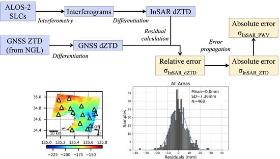
InSAR originally observes the phase change , which reflects the differences in microwave propagation path lengths. is the linear sum of phase changes due to several factors, as shown in Equation (1). Regarding the neutral atmospheric delay, InSAR observes the relative difference in atmospheric delays between two acquisition times. In this study, we estimated the “InSAR zenith total delay difference” (), whose offset was calibrated using the “GNSS zenith total delay difference” () according to the formulae provided in previous studies [19,20]. Hereinafter, “InSAR initial value” () denotes the phase delay in the zenith direction converted from the satellite line-of-sight direction using the incidence angle and a simple trigonometric function. was derived through the following equation as follows:
where is the colocation point number of the GNSS and InSAR observation point in the target area. Here, it should be noted that InSAR observations reflect the delay along the line-of-sight (narrow tube), but GNSS ZTDs reflect the average of the delay within the inverse cone space above GNSS stations. This indicates that GNSS-derived atmospheric values are representative values within the inverse cone, whose radius at the tropopause (approximately 12 km around Japan) was approximately 100 km, with the cut-off angle of 7 degrees, in our case. On the other hand, the InSAR phase is only affected by the atmosphere along the microwave path, indicating that the InSAR PWV signal reflects the atmospheric heterogeneity within a narrow tube (radius ranging from a few to a hundred meters depending on multilooking and filtering processes) between the ground and the satellite. In this context, we should keep in mind that the spatial representativeness of InSAR PWV observation is intrinsically different from that of GNSS. Therefore, to compensate for this representativeness gap between InSAR and GNSS, even if only slightly, we applied significantly large multilooking and strong spatial filtering to all interferograms, resulting in values of the actual spatial resolution of several hundred meters or larger. Details of the InSAR processing are described in Section 4.1.
The must be calibrated to be converted into . The amount of an offset in a specific scene () is determined by the non-weighted average of estimated differences between the and at each station within the scene:
where and represent the ZTD observed by GNSS at times closest to the reference SAR observation and the secondary one, respectively. Using the estimated offset, we could obtain at an arbitrary pixel () by adding it to :
The standard deviation of residuals between and represents the relative error of from . As previous studies that evaluated measurement errors of other kinds of water vapor measurement techniques estimated these absolute errors by assuming the radiosonde observation technique as the most accurate, our study finally estimated the absolute error of the L-band InSAR PWV measurement by considering the radiosonde-derived PWV values as the true value. In sum, we considered the relative error of the InSAR PWV measurement against the radiosonde PWV measurement as the absolute error of the InSAR PWV observation. To estimate the standard deviation of residuals between and , we defined the residual () at a location between and as follows:
Then, its standard deviation () was calculated as follows:
where represents the mean of in a specific interferogram.
Then, we could reasonably assume that errors of and had no correlation and could be set as equal () since the time interval of these two observations was larger than 14 days, which is the recurrence interval of the ALOS-2 satellite. Under this assumption, we could express the error of using the law of error propagation as follows:
In our study, we adopted as 17.0 mm, as obtained in a previous study [27].
The absolute dZTD error of InSAR, which is the relative error against the radiosonde dZTD, is equal to the root of the square sum of (1) the relative error of the GNSS dZTD (), (2) the processing error of the GNSS ZTD (), and (3) the relative error of from (). Using Equation (20), can be expressed as follows:
Here, is fixed as 3.0 mm, which is the rough average from the processed GNSS ZTD data [28].
As Equation (21) represents the error of difference of two InSAR ZTD observations, its decomposition into the error of InSAR ZTD measurements at a single observation is required. Assuming that there is no correlation between atmospheric delays in each SAR acquisition time, the error of InSAR ZTD () can be introduced using the law of error propagation from in Equation (21). From the assumption, standard deviations (errors) of InSAR ZTDs at reference and secondary observations can be regarded as equal. As the is derived from two independent InSAR ZTDs (), can be decomposed as the root of the square sum of two standard deviations of . This can be expressed as follows:
To estimate the PWV error, we further needed to decompose into errors of dry and wet components. From the relationship between ZWD and ZTD, the error of InSAR ZWD () can be expressed as follows:
where is the estimation error of ZHD in Equation (7), and as introduced in Section 2, we set this value as 2.41 mm from the previous study [25]. Using Equation (23), we could remove the contribution of the dry air and obtain the error of InSAR ZWD measurements, which was used to obtain the error of the InSAR PWV measurements.
The relationship between ZWD and PWV is provided by Equations (10) to (13). According to [24], the PWV conversion factor Π can be estimated with good accuracy using the surface temperature. As the sensitivity of Π to is small, in this study, we used a fixed value of surface temperature, , which was estimated from the average temperature from June to September (hereafter referred to as the wet season) in 2020 in the Kyushu region, where heavy rainfall events are especially likely to occur in this season. The reason that we chose this period is that a large amount of SAR data we used were obtained in Kyushu during the wet season. Specifically, we used , and thus the absolute error of the InSAR PWV (), which we aimed to estimate, is expressed as follows:
4. Data
4.1. InSAR Data
The SAR data used in this study were acquired by the phased array L-band SAR 2 (PALSAR-2) onboard the Advanced Land Observing Satellite-2 (ALOS-2), which is operated by the Japan Aerospace Exploration Agency (JAXA). The observation mode used here was the strip map (SM) ultrafine mode with a spatial resolution of 3 m in both range and azimuth directions. The single SAR scene in the SM mode covers an area of approximately 50 × 50 km2. All interferograms were generated from level-1.1 Single Look Complex (SLC) images using the Radar Interferometry Calculation Tools (RINC) software ver. 0.41r [29]. was estimated from the high-precision satellite orbit data provided by JAXA, and was removed by simulating the terrain fringes with the 3-arcsecond Shuttle Radar Topography Mission (SRTM) DEM provided by the United States Geological Survey (USGS). Multilook processing resulted in an improvement in the interferometric coherence by sacrificing the spatial resolution of the InSAR data to approximately 100 m in both range and azimuth directions. We used the Goldstein and Werner filter with the alpha value of 0.7 and the filter window size of 32 pixels to reduce small-scale phase noises [30]. After removing these phase contributions, we could obtain the phase difference due to the neutral atmospheric delay. The statistical-cost, network-flow phase-unwrapping algorithm (SNAPHU) software was used for phase unwrapping [31]. For the calculation of residuals, we used , where the interferometric coherence was greater than 0.3.
The ionospheric delay was estimated and removed by the range split-spectrum method (SSM) [32]. As Gomba et al. [32] demonstrated, SSM can largely reduce ionospheric delay phase contaminations by splitting the range spectrum into higher and lower parts. Although several papers have reported the effectiveness of SSM to mitigate the ionospheric delay signal [33,34,35], to the best of our knowledge, none of the reviewed papers reported its statistical performance. According to the derivation of Gomba et al. [32], the theoretical estimation accuracy of the ionospheric delay by SSM is an order of centimeters or less depending on the interferometric coherence and the multilooking size. We visually checked all interferograms and found that the application of SSM to interferograms with serious ionospheric delay contaminations showed a significant reduction, especially for long-wavelength phase variations.
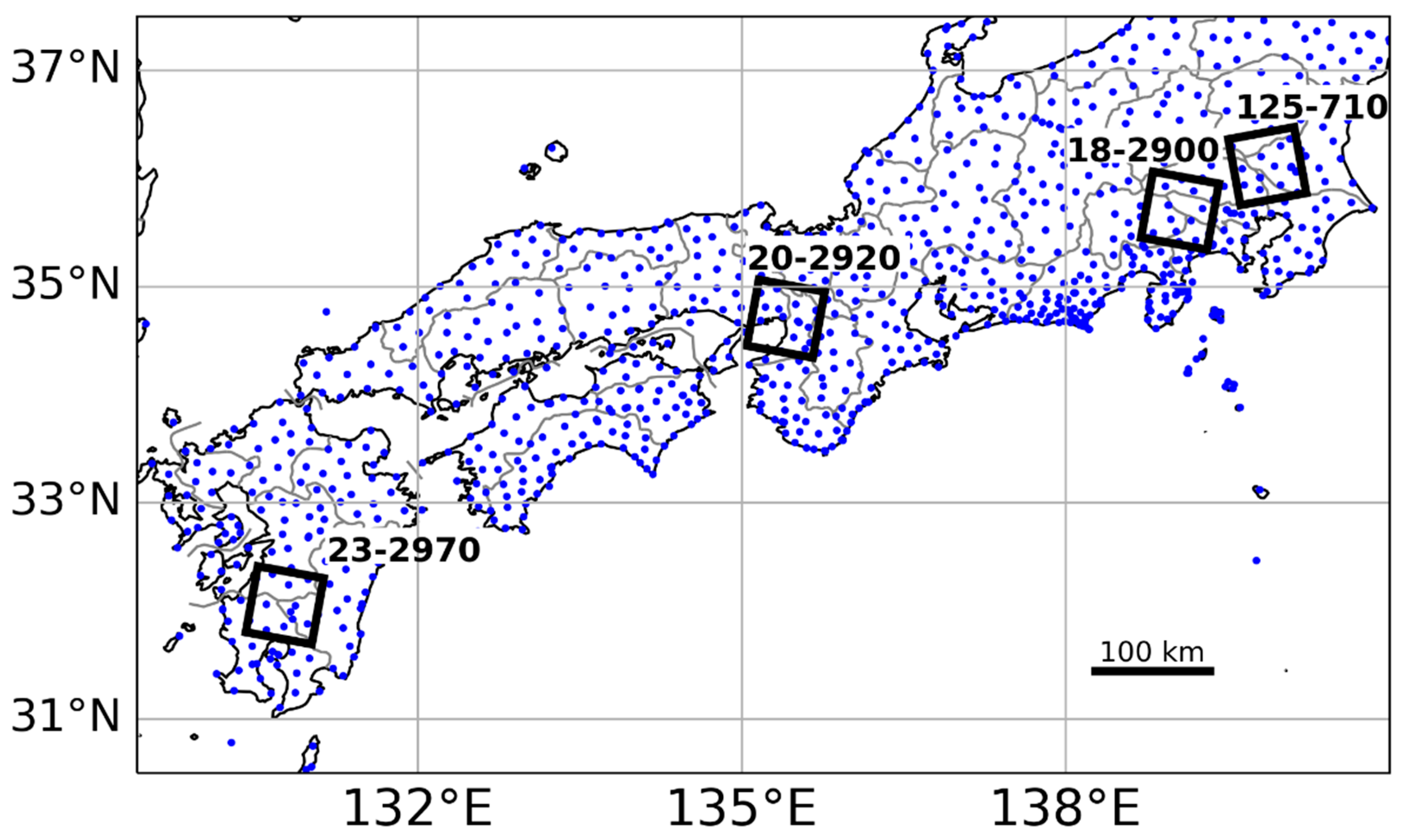
We selected four areas in Japan—southern Ibaraki, western Tokyo, Osaka and southern Kyushu—where a significant number of GNSS stations and ALOS-2 SM1 mode SLCs are available (Figure 1). The orbit is ascending in southern Ibaraki and descending in the other areas. Detailed information of the SAR observations is summarized in Table 1.
Japan is well known as a tectonically active area, and thus several kinds of phenomena, such as earthquakes, land subsidence, and volcanic activities, cause surface deformation. In this study, we assumed that there was no surface displacement () as no large earthquakes (>M6) were reported among all pairs of reference and secondary SAR acquisitions. Note that recent studies reported that earthquakes with magnitudes not only larger than 6 but also smaller than 6 can cause geodetically detectable surface displacements if source depths are close to the surface (depths of a few kilometers) [36,37,38]. To assess the possible impacts due to both larger- and smaller-magnitude earthquakes, we checked the earthquake source catalog developed by the Japan Meteorological Agency. As a result, we confirmed that all interferograms used in this study contain no possible impacts due to co-seismic fault slips. In addition, as we chose interferometric pairs by using two subsequently acquired SLCs, all interferograms have time intervals of shorter than 210 days (most parts of the interferograms have time intervals shorter than four months), which would be significantly short to neglect secular surface displacements, such as the plate tectonic motion and land subsidence (ranging from a few millimeters per year to centimeters per year).
4.2. GNSS Data
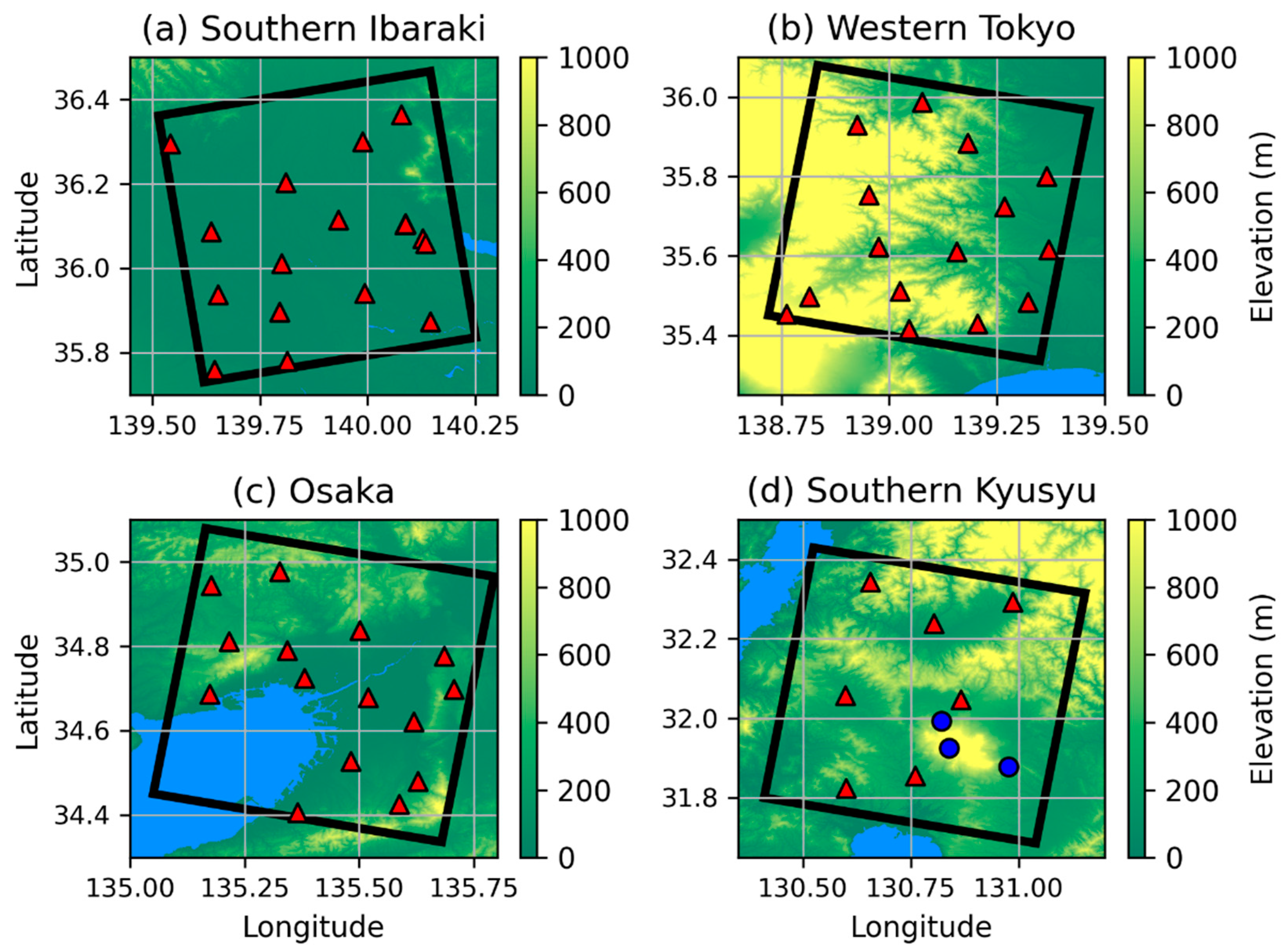
GNSS data were derived from the GNSS Earth Observation Network System (GEONET), the operational GNSS network in Japan. We used the 5 min-interval tropospheric parameters estimated by the Geodesy Laboratory at the University of Nevada (NGL) [28]. The analysis method for the GNSS was the precise point positioning method using the International GNSS service precise orbit information and Earth rotation parameters. In order to avoid the effect of surface displacements caused by volcanic activity, GNSS observation data near Mt. Kirishima in southern Kyushu (blue circles in Figure 2d) were excluded in our analysis. shown in Equation (21) is provided by NGL. As a result, there were 18 stations in southern Ibaraki, 15 stations in western Tokyo and Kanagawa, 15 stations in Osaka and 7 stations in southern Kyushu (red triangles in Figure 2).
5. Result
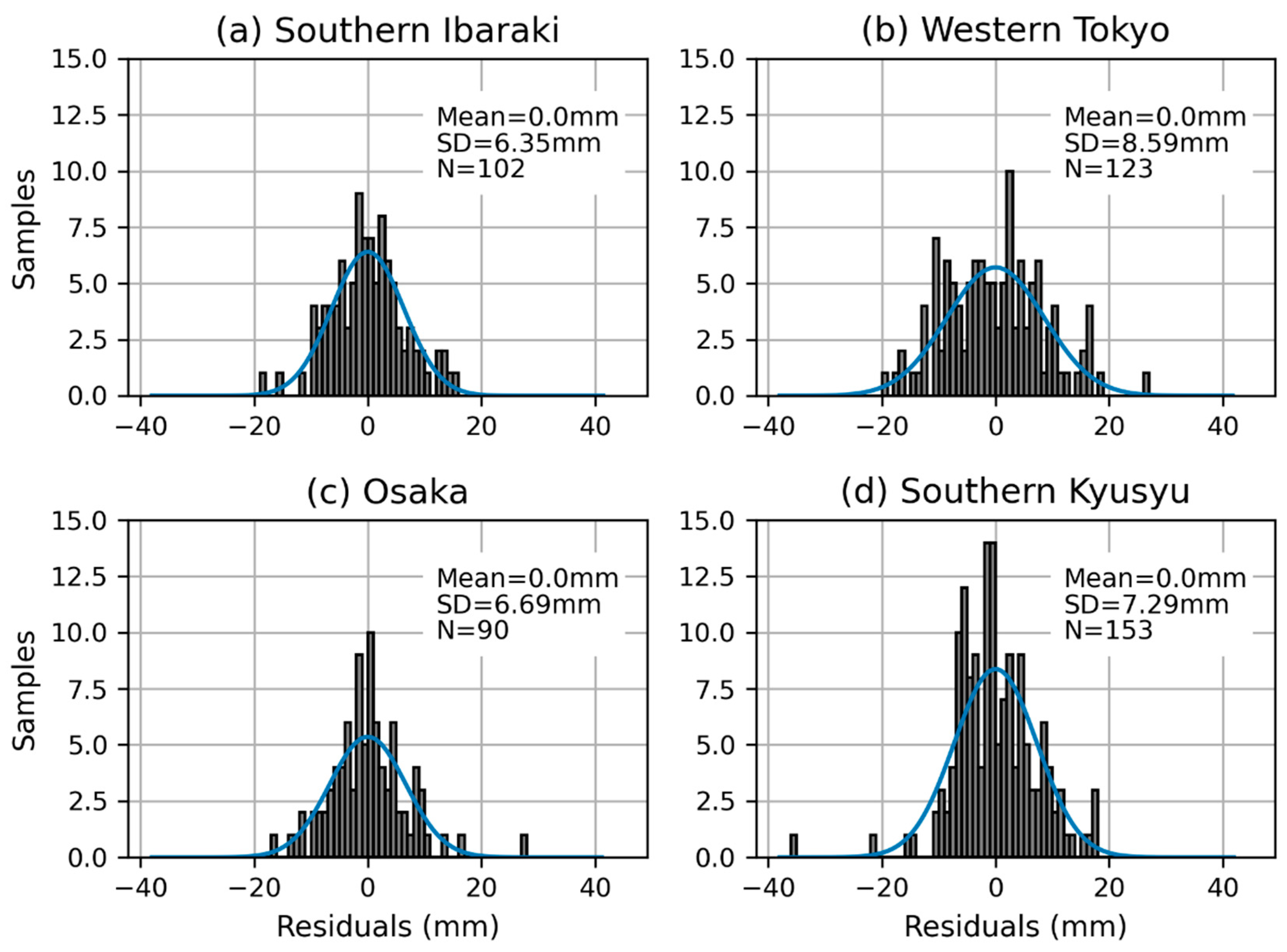
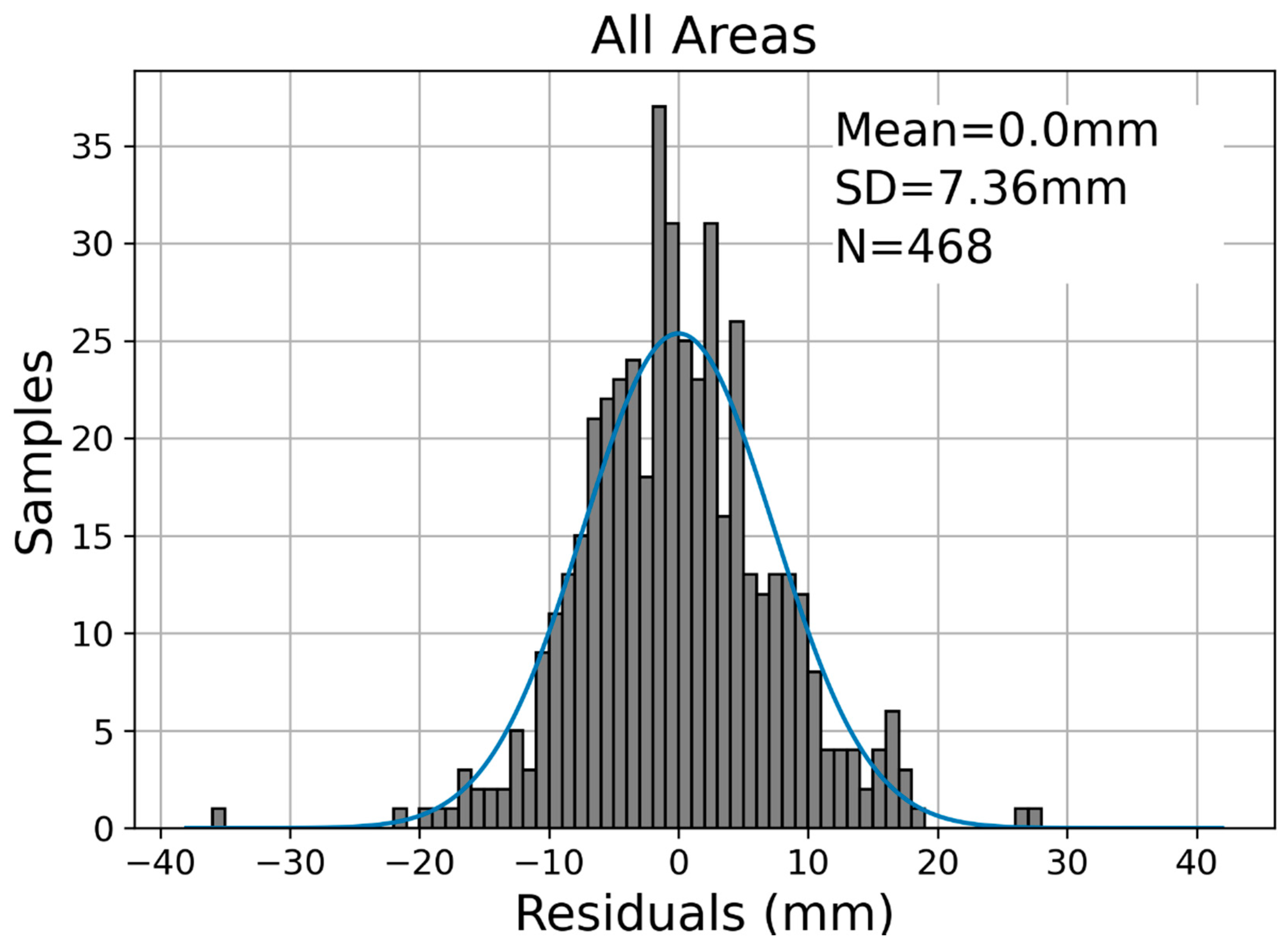
Figure 3 shows the distribution of residuals between and () in each area. The average values of residuals were 0.00 mm in each area. Standard deviations of were 6.35 mm in southern Ibaraki, 8.59 mm in western Tokyo, 6.69 mm in Osaka and 7.29 mm in southern Kyusyu, respectively. We also plotted the distribution of the residuals between and , combining all four areas in Figure 4. For the residuals of all four areas, the mean and standard deviation () became 0.00 and 7.36 mm, respectively. Based on the estimated standard deviation of the residuals including all areas, we evaluated the errors in Equations (21) (), (22) (), (23) () and (26) () step by step using the error propagation theory. First, we calculated the absolute error of InSAR dZTD () using Equation (21), resulting in 25.50 mm based on GNSS processing and the ZTD error values introduced in Section 3. In the next step, we calculated in Equation (22), which was estimated as 18.03 mm. After calculating using the ZHD error () through Equation (23), we could finally obtain the absolute error of InSAR PWV () as 2.96 mm through Equation (24). The estimated was slightly larger than the PWV errors of other observation techniques evaluated in previous studies [12,20,39,40,41] (Figure 5 and Figure 6).
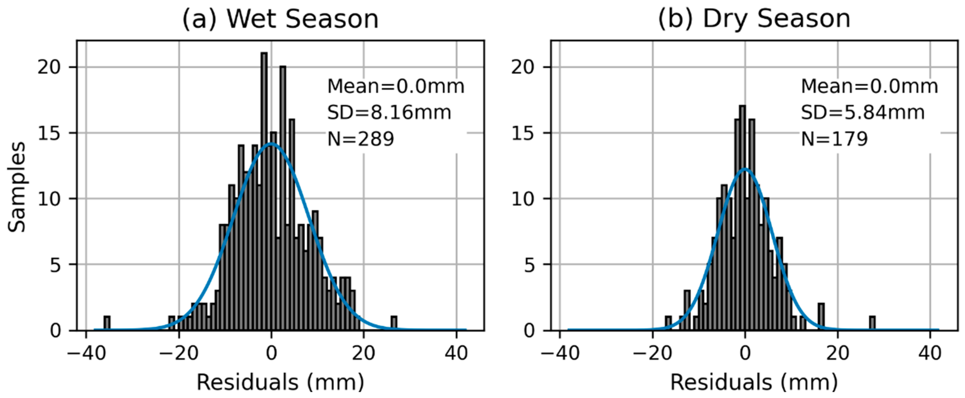
In the previous study [42], the PWV in July was greater than in January in Japan. Shoji [42] also showed the same tendency in the root mean square (RMS) difference between the GNSS and radiosonde PWV. Moreover, the GNSS PWV has a seasonal variation in Japan [43]. We checked whether the error of the InSAR PWV becomes larger in the wet season as with the error of the GNSS PWV. Figure 7 shows the distribution of data that were acquired during the wet season. As a result, the mean of GNSS ZTD was larger in the wet season than in other months (hereafter referred to as the dry season) in our case. The mean and standard deviation of were 0.00 and 8.16 mm, respectively, during the wet season. in the wet season became 2.99 mm. On the other hand, the mean and standard deviation of were 0.00 and 5.84 mm, respectively, in the dry season. in the dry season became 2.91 mm. Our results indicate that was larger in months when the GNSS ZTD was also larger than that in other months. We concluded that was greater in the wet season than that in the dry season.
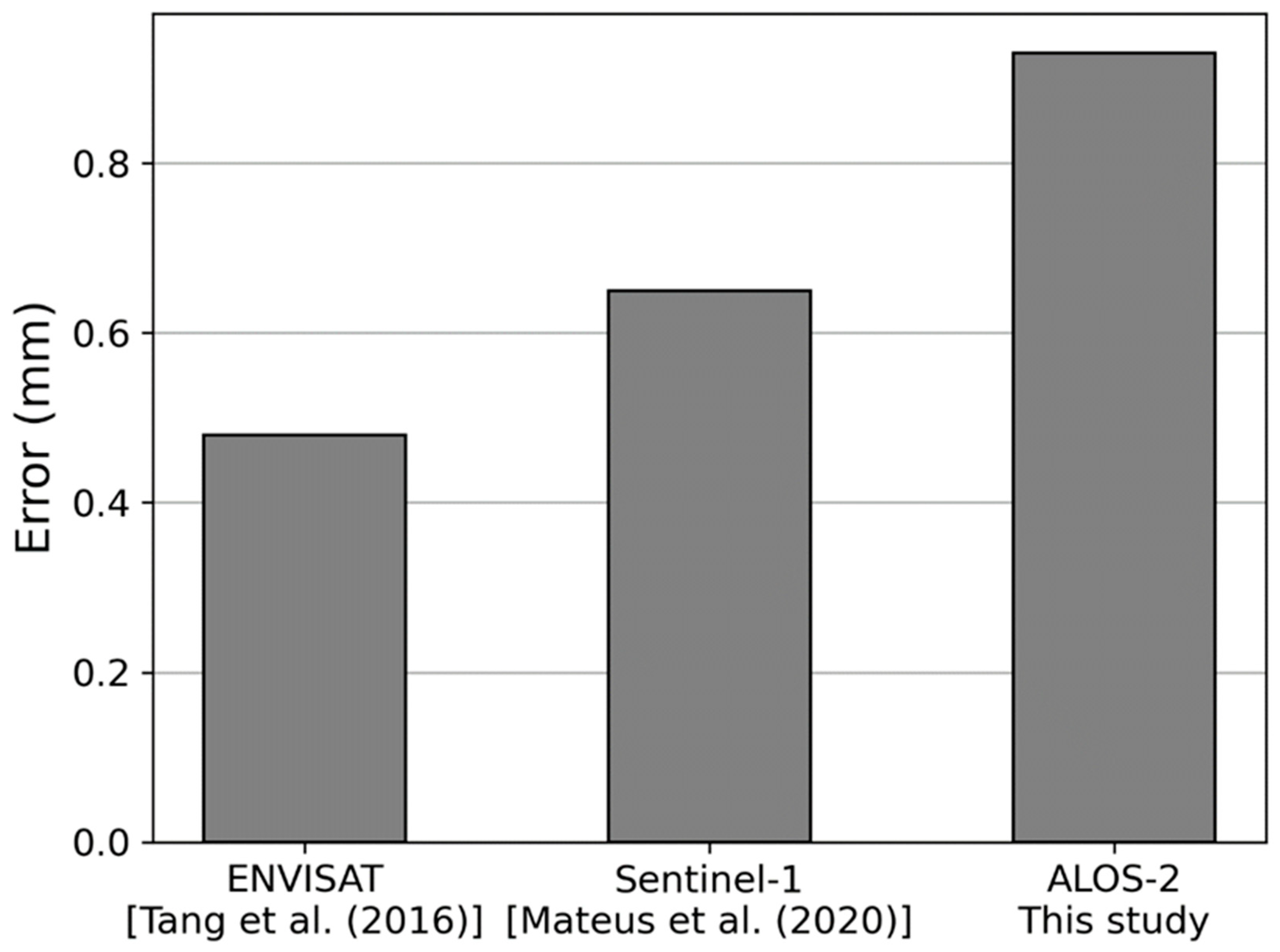
We compared the error of the L-band InSAR PWV () estimated from this study with that of the C-band InSAR PWV estimated by other studies [12,20] (Figure 5). Note that previous studies only estimated the standard deviation of residuals between and . Therefore, Figure 6 shows the relative PWV errors of InSAR against GNSS. The error of the L-band InSAR PWV compared with the GNSS PWV () can be estimated by Equation (24) with (=7.4mm) instead of . In the previous study [20], the ENVISAT difference PWV error was 0.675 mm, which was the average of the mean absolute error (MAE) of difference PWVs between InSAR and GNSS for 10 interferograms in the United States (US). Here, we divided their PWV errors by using Equation (22) and replaced the ZTD with PWV to obtain the above error values, resulting in the ENVISAT PWV error in [20] becoming 0.48 mm. The Sentinel-1 PWV error was 0.65 mm, which was the average of the root mean square error (RMSE) between the InSAR and GNSS PWV of 10 interferograms in the US [12]. The L-band InSAR PWV error in this study was found to be 0.93 mm by solving the following equation:
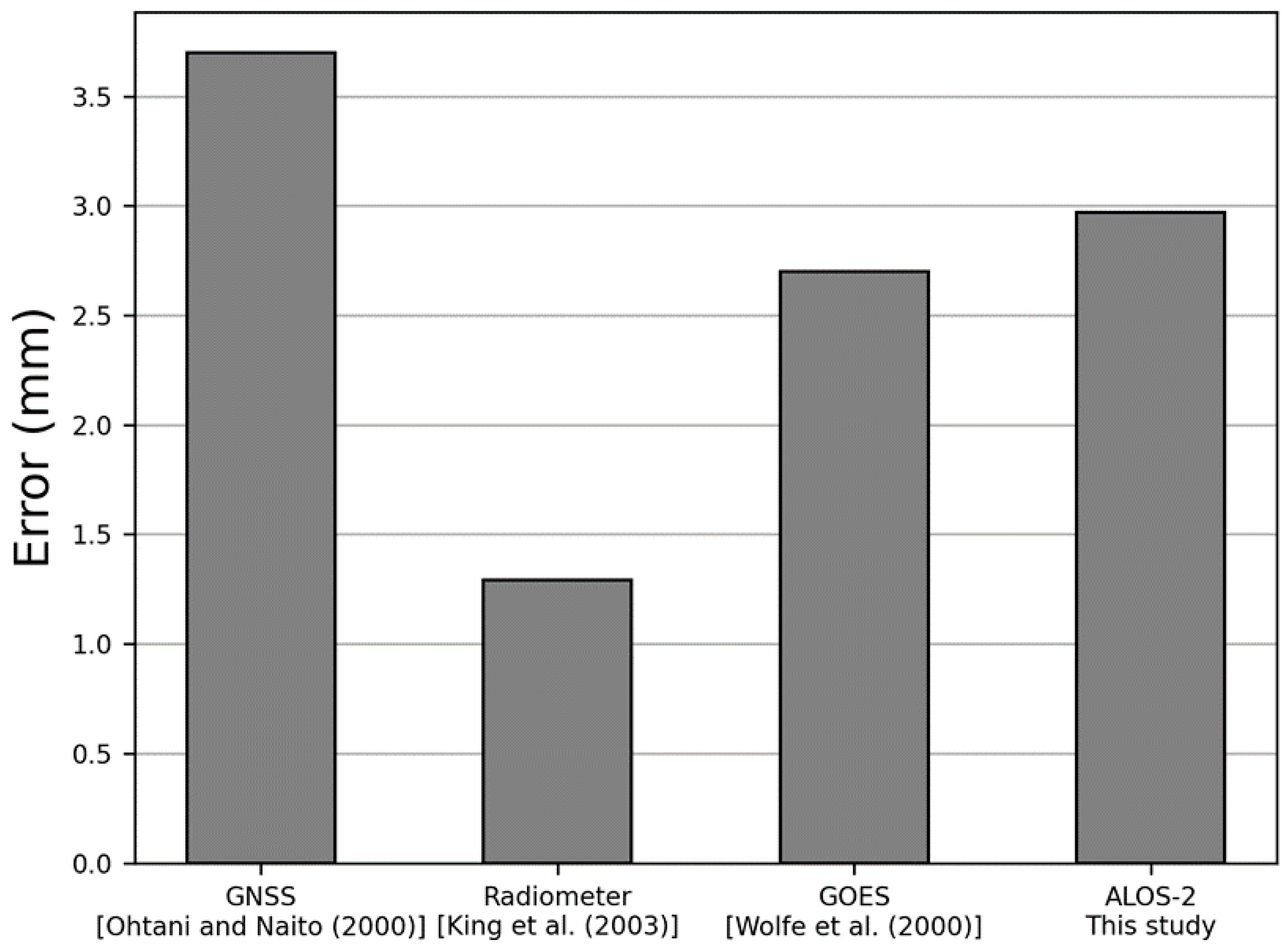
Figure 6 summarizes the observation errors of other kinds of PWV observations and the error of the L-band InSAR PWV estimated in this study. These observation errors are relative errors to the radiosonde observation. In [39], the GNSS error was 3.7 mm, which was the RMSE with 10 radiosonde stations observed for one year in Japan. The radiometer error was 1.29 mm, which was the RMSE against the radiosonde PWV in the US [40]. The Geostationary Operational Environmental Satellite (GOES) error was 2.7 mm, which was the RMSE against the radiosonde PWV in the US [41]. Comparing the estimated L-band InSAR PWV error with those of other techniques, as shown in Figure 6, the L-band InSAR PWV observation showed relatively worse accuracy than others. Nonetheless, the PWV error level of 2.96 mm in the L-band InSAR would be too small for meteorological use as PWV in Japan ranges from 10 to 50 mm in ordinary conditions, and sometimes exceeds 80 mm in extreme weather conditions [43].
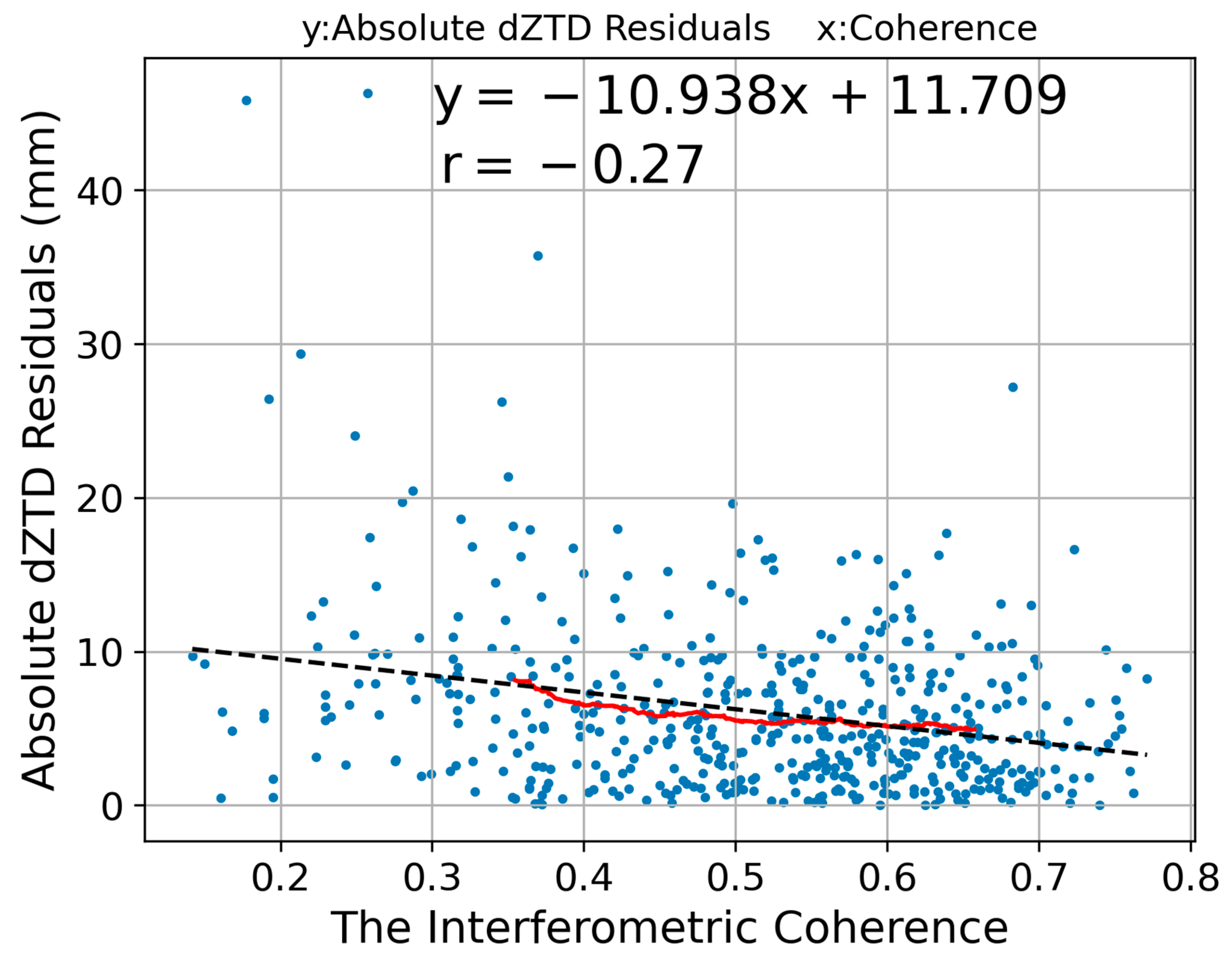
We investigated the relationship between the interferometric coherence and the InSAR atmospheric observation accuracy. Although we used InSAR observation values with an interferometric coherence greater than 0.3 to estimate the amount of offset in a specific InSAR scene, we also plotted the absolute values of estimated with a coherence lower than 0.3. Figure 8 shows the scatterplot of absolute dZTD residuals () as a function of the interferometric coherence. We also plotted the regression line and the moving average line (the black dashed line and the solid red line in Figure 8) to visually elucidate the relationship between the interferometric coherence and absolute values of estimated . The correlation coefficient between the scatterplot of absolute dZTD residuals and the coherence was −0.27, indicating a weak negative correlation between the residuals and the coherence. If the interferometric coherence is lower, InSAR observation becomes less precise, which may be due to the decorrelation noise.
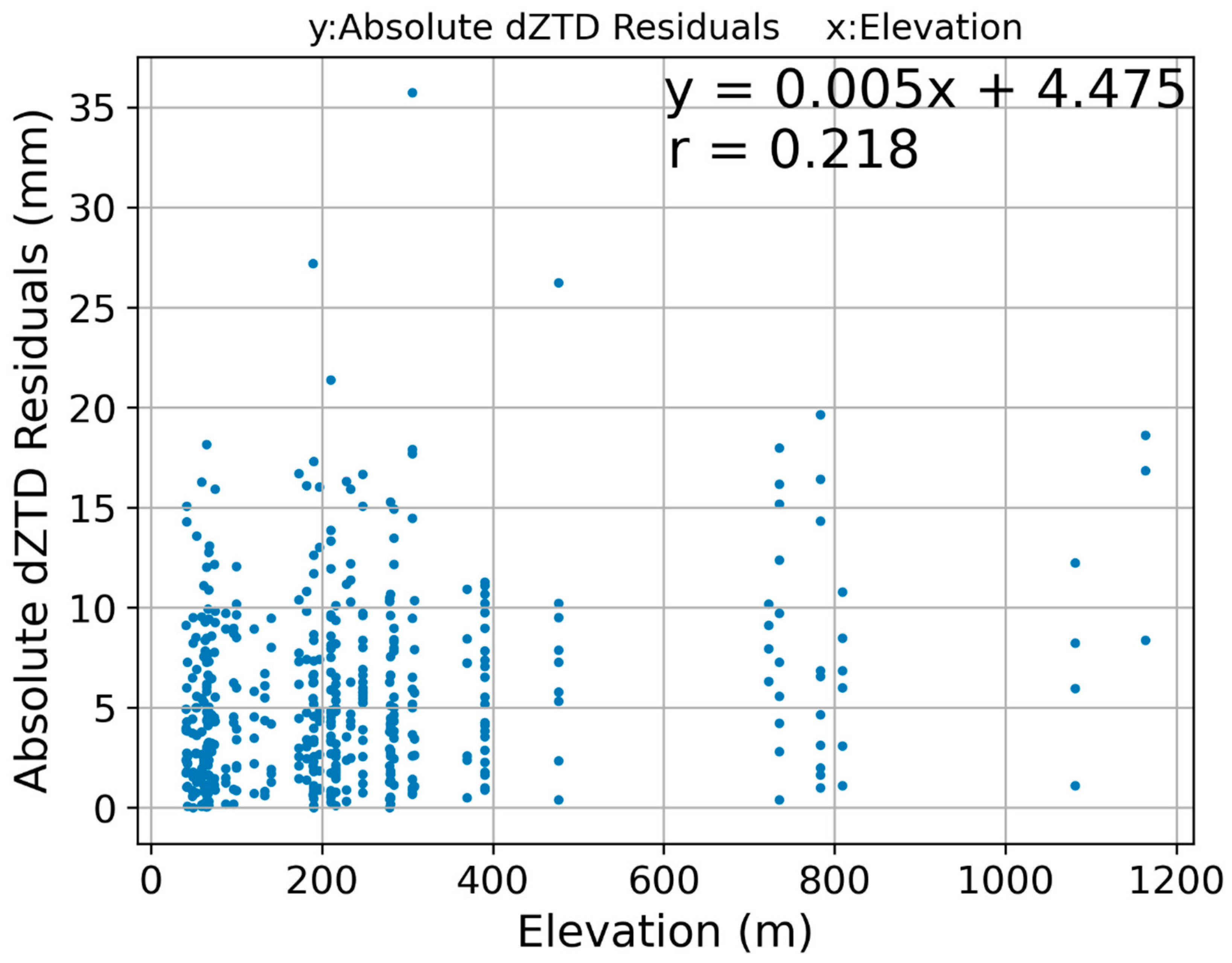
In addition, we investigated the height dependence of the ZTD residual between InSAR and GNSS. Figure 9 shows the scatter plot of the residuals of all four areas as a function of observation altitude and a fitting line with a correlation coefficient of 0.218. Similar to the relation between the interferometric coherence and absolute values of estimated , we found a weak positive correlation between the elevation and absolute values of estimated . Possible explanations for the existence of this weak positive correlation may be that (1) at higher altitudes (around 1000–2000 m), atmospheric turbulence is more severe and highly variable, and (2) some GNSS stations in mountainous areas were affected by topographic configurations by, for example, blocking lower-elevation microwave paths. However, these possible explanations are only speculation, and the number of samples and survey areas seem to be insufficient to derive any conclusions. Therefore, the height dependence of the ZTD residuals and its mechanism should be further investigated in future works.
6. Discussion
The comparison of different seasons in Figure 7 shows interesting features. during the wet season was 1.50 times larger than that during the dry season. This result indicated that in the wet season, when the ZTD was large, the discrepancy between GNSS and InSAR atmospheric observation also increased. Furthermore, the shapes of the histograms in Figure 7 visually suggest that the shape in the wet season deviated further from the fitted Gaussian distribution than that in the dry season. InSAR observations reflect the delay along the line-of-sight (within a narrow tube extended between the satellite and the ground pixel), but GNSS ZTDs reflect the average of the delay within the inverse cone space above GNSS stations. These different characteristics may affect ZTD observation when atmospheric water vapor largely varies over small distances (for instance, orders of from hundreds to thousands of meters). If this difference was a reason that the residual became greater in the wet season than in the dry season, then water vapor may severely fluctuate in the wet season compared to in the dry season.
We evaluated the relative error of the L-band InSAR PWV against the GNSS as 0.93 mm, which was comparatively worse than the C-band InSAR PWV error in previous studies [12,20]. We summarized possible factors of the difference between previous studies and our study as follows: (1) We performed a comparison between GNSS data and a collocated InSAR pixel, but the average of multiple InSAR pixels (for example, the radius of a few kilometers) surrounding GNSS stations was used in previous studies. As our method compared the dZTD of one InSAR pixel (resolution of several hundred meters or larger by multilooking and filtering) with GNSS dZTD, residual pixel-scale noises may affect the error level estimation. Here, note that extending the averaging radius would make the interpretation more complex in terms of the pixel height and the associated stratified delay effect. Especially in mountainous areas, if we set a large radius for averaging, the averaged pixel value would make the InSAR delay value more suitable for the comparison to GNSS in terms of horizontal representativeness but may represent a delay value at a different height due to variable topography height. This causes another problem for the comparison of InSAR and GNSS. Therefore, we need to determine the averaging radius carefully. According to our understanding, both too large and too small radii would be inappropriate, although we do not have an idea of how to determine the radius for averaging. (2) While we removed from the total phase differences of the L-band InSAR, it should be noted that our ionospheric correction cannot perfectly remove the effect of the ionosphere, and thus the residual in the ionospheric correction may have had a negative impact on the InSAR PWV error estimation in this study. Previous studies have not removed it as they considered its effect to be negligible as in the case of C-band InSAR, which has a higher microwave frequency and, thus, lower ionospheric phase contamination. (3) Previous studies [12,20] used SAR images acquired during drier seasons than the Japanese summer season. The larger the PWV values are, the larger the InSAR PWV errors might be [42]. On the other hand, there is no difference between the GNSS atmospheric processing in our study and that in the previous two studies. Due to the above-described reasons, the error of L-band InSAR PWV estimated in this study may, to some extent, become larger than the error of C-band InSAR.
We also compared the L-band InSAR PWV error with other PWV observation errors in Figure 6. Contrary to our intuition, the GNSS PWV error was larger than the L-band InSAR PWV error evaluated in this study. Among the reasons for such a contradiction may be that we could not compare the InSAR observation with the radiosonde directly as no available data existed; however, the estimated L-band InSAR error included the GNSS observation error. Therefore, our estimated InSAR error included errors of both the GNSS and the radiosonde, resulting in the tendency towards larger estimation to some extent. Nevertheless, the estimated L-band InSAR PWV error was approximately the same order as other PWV observation errors. In the future, the InSAR PWV error should be directly compared with radiosonde PWV. Another reason for this may be that the GNSS PWV error was derived at the end of the 20th century. Recently, GNSS processing techniques have been further improved, and the number of available GNSS satellites is increasing. Therefore, the GNSS PWV observation would be more accurate than that at the time of the previous study.
We evaluated the relationship between and the interferometric coherence. In Figure 8, the smaller the interferometric coherence was, the larger the absolute value () tended to be. Especially in the range of coherence values lower than 0.3, the number of samples was small, and there were some extraordinarily large . Our method did not use pixels with a coherence of less than 0.3 for offset estimation. Therefore, the absolute values of with a coherence of less than 0.3 tended to largely deviate and may have had bias. It is important to define the threshold of the interferometric coherence appropriately when estimating offsets.
7. Conclusions
We estimated the dZTD distribution using L-band ALOS-2 InSAR data and calculated the residuals between and using the error propagation theory. The estimated standard deviation of residuals was 7.36 mm, which was used to estimate the observation error of PWV derived from InSAR data, which was finally found to be 2.96 mm. The estimated L-band InSAR PWV error was comparable to that of other InSAR observations evaluated in previous studies. We investigated the dependences of the observation season and altitude and found that the standard deviation of the residual increased in the wet season, which may be due to the high variability and a larger amount of water vapor in this season. The height dependence was not suggested in our analysis. This study clarified that the InSAR water vapor observation using L-band InSAR has significant accuracy compared to C-band InSAR, which showed its usefulness for the data assimilation into meso-scale weather prediction [7,9,18,44], indicating that L-band InSAR also has the potential for improving the precipitation forecast. At present, there are no experiments on the precipitation forecast using the L-band InSAR data assimilation. In the near future, high-spatial resolution water vapor mapping by InSAR may be utilized for operational meso-scale weather forecasting to enhance its prediction ability, especially against localized severe rainfall. The number of SAR satellites from both governmental space agencies and private companies is expected to increase in the coming decades, and thus, more InSAR data will be available for meteorological applications. The use of high-spatial and -temporal density InSAR data for weather forecasting would improve precipitation prediction for localized heavy rainfall, which is currently difficult to predict accurately, and contribute to mitigating the social damages caused by hydrological disasters related to heavy rainfall.
Author Contributions
K.M. performed data analysis and produced all the results. K.M. drafted the manuscript. Y.K. contributed to the conceptualization and discussion of the study and reviewed the manuscript. All authors conceived the study and approved the manuscript. All authors have read and agreed to the published version of the manuscript.
Funding
This research received no external funding.
Institutional Review Board Statement
Not applicable.
Informed Consent Statement
Not applicable.
Data Availability Statement
The data presented in this study are available on request from the corresponding author.
Acknowledgments
PALSAR-2 SLC data were shared among the PALSAR Interferometry Consortium to Study our Evolving Land Surface (PIXEL). The data were provided by the Japan Aerospace Exploration Agency (JAXA) under a cooperative research contract with the Earthquake Research Institute of the University of Tokyo. The GEONET GNSS data were originally provided by the Geospatial Authority of Japan, and we used processed products from the Nevada Geodetic Laboratory, University of Nevada. We acknowledge P. Mateus and an anonymous reviewer for their helpful and constructive comments.
Conflicts of Interest
The authors declare no conflict of interest.
References
- Ross, R.J.; Elliott, W.P. Tropospheric Water Vapor Climatology and Trends over North America: 1973-93. J. Climat. 1996, 9, 3561–3574. [Google Scholar] [CrossRef] [Green Version]
- Vonder Haar, T.H.; Bytheway, J.L.; Forsythe, J.M. Weather and climate analyses using improved global water vapor observations. Geophys. Res. Lett. 2012, 39, L15802. [Google Scholar] [CrossRef]
- Shi, J.B.; Xu, C.Q.; Guo, J.M.; Gao, Y. Real-Time GPS Precise Point Positioning-Based Precipitable Water Vapor Estimation for Rainfall Monitoring and Forecasting. IEEE Trans. Geosci. Remote Sens. 2015, 53, 3452–3459. [Google Scholar] [CrossRef]
- Manandhar, S.; Lee, Y.H.; Dev, S. GPS Derived PWV for Rainfall Monitoring. In Proceedings of the International Geoscience and Remote Sensing Symposium (IGARSS), Beijing, China, 10–15 July 2016; pp. 2170–2173. [Google Scholar] [CrossRef]
- Yao, Y.; Shan, L.; Zhao, Q. Establishing a method of short-term rainfall forecasting based on GNSS-derived PWV and its application. Sci. Rep. 2017, 7, 12465. [Google Scholar] [CrossRef] [PubMed]
- Emanuel, K.; Raymond, D.; Betts, A.; Bosart, L.; Bretherton, C.; Droegemeier, K.; Farrell, B.; Fritsch, J.M.; Houze, R.; Le Mone, M.; et al. Report of the First Prospectus Development Team of the U.S. Weather Research Program to NOAA and the NSF. Bull. Am. Meteorol. Soc. 1995, 76, 1194–1208. [Google Scholar]
- Mateus, P.; Tomé, R.; Nico, G.; Catalão, J. Three–Dimensional Variational Assimilation of InSAR PWV Using the WRFDA Model. IEEE Trans. Geosci. Remote Sens. 2016, 54, 7323–7330. [Google Scholar] [CrossRef]
- Kinoshita, Y.; Shimada, M.; Furuya, M. InSAR observation and numerical modeling of the water vapor signal during a heavy rain: A case study of the 2008 Seino event, central Japan. Geophys. Res. Lett. 2013, 40, 4740–4744. [Google Scholar] [CrossRef]
- Pierdicca, N.; Maiello, I.; Sansosti, E.; Venuti, G.; Barindelli, S.; Ferretti, R.; Gatti, A.; Manzo, M.; Monti-Guarnieri, A.V.; Murgia, F.; et al. Excess Path Delays From Sentinel Interferometry to Improve Weather Forecasts. IEEE J. Sel. Top. Appl. Earth Obs. Remote Sens. 2020, 13, 3213–3228. [Google Scholar] [CrossRef]
- Cao, Y.; Li, Z.; Duan, M.; Wei, J. High-Resolution Water Vapor Maps Obtained by Merging Interferometric Synthetic Aperture Radar and GPS Measurements. J. Geophys. Res. Atmos. 2020, 126, 1. [Google Scholar] [CrossRef]
- Mateus, P.; Nico, G.; Tomé, R.; Catalão, J.; Miranda, P.M.A. Experimental Study on the Atmospheric Delay Based on GPS, SAR Interferometry, and Numerical Weather Model Data. IEEE Trans. Geosci. Remote Sens. 2013, 51, 6–11. [Google Scholar] [CrossRef]
- Mateus, P.; Catalão, J.; Nico, G.; Benevides, P. Mapping Precipitable Water Vapor Time Series From Sentinel–1 Interferometric SAR. IEEE Trans. Geosci. Remote Sens. 2020, 58, 1373–1379. [Google Scholar] [CrossRef]
- Zebker, H.A.; Rosen, P.A.; Hensley, S. Atmospheric effects in interferometric synthetic aperture radar surface deformation and topographic maps. J. Geophys. Res. 1997, 102, 7547–7563. [Google Scholar] [CrossRef]
- Kinoshita, Y.; Morishita, Y.; Hirabayashi, Y. Detections and simulations of tropospheric water vapor fluctuations due to trapped lee waves by ALOS-2/PALSAR-2 ScanSAR interferometry. Earth Planet Space 2017, 69, 1–15. [Google Scholar] [CrossRef] [Green Version]
- Kursinski, E.R.; Hajj, G.A. A comparison of water vapor derived from GPS occultations and global weather analyses. J. Geophys. Res. 2001, 106, 1113–1138. [Google Scholar] [CrossRef]
- Shoji, Y.; Yamauchi, H.; Mashiko, W.; Sato, E. Estimation of local-scale precipitable water vapor distribution around each GNSS station using slant path delay. SOLA 2014, 10, 29–33. [Google Scholar] [CrossRef] [Green Version]
- Hanssen, R.F.; Weckwerth, T.M.; Zebker, H.A.; Klees, R. High-Resolution Water Vapor Mapping from Interferometric Radar Measurements. Science 1999, 283, 1297–1299. [Google Scholar] [CrossRef] [PubMed] [Green Version]
- Mateus, P.; Miranda, P.M.A.; Nico, G.; Catalao, J. Continuous multitrack assimilation of Sentinel-1 precipitable water vapor maps for numerical weather prediction: How far can we go with current InSAR Data? J. Geophys. Res. Atmos. 2021, 126, e2020JD034171. [Google Scholar] [CrossRef]
- Mateus, P.; Nico, G.; Catalão, J. Can spaceborne SAR interferometry be used to study the temporal evolution of PWV? Atmos. Res. 2013, 119, 70–80. [Google Scholar] [CrossRef]
- Tang, W.; Liao, M.; Zhang, L.; Li, W.; Yu, W. High-spatial-resolution mapping precipitable water vapor using SAR interferograms, GPS observations and ERA-Interim reanalysis. Atmos. Meas. Tech. 2016, 9, 4487–4501. [Google Scholar] [CrossRef] [Green Version]
- Bevis, M.; Businger, S.; Herring, T.A.; Rocken, C.; Anthes, R.A.; Ware, R.H. GPS meteorology: Remote Sensing of Atmospheric Water Vapour Using the Global Positioning System. J. Geophys. Res. 1992, 97, 15787–15801. [Google Scholar] [CrossRef]
- Ciraolo, L.; Azpilicueta, F.; Brunini, C.; Meza, A.; Radicella, S.M. Calibration errors on experimental slant total electron content (TEC) determined with GPS. J. Geod. 2007, 81, 111–120. [Google Scholar] [CrossRef]
- Thayer, G. An improved equation for the radio refractive index of air. Radio Sci. 1974, 9, 803–807. [Google Scholar] [CrossRef]
- Bevis, M.; Businger, S.; Chiswell, S.; Herring, T.A.; Anthes, R.A.; Rocken, C.; Ware, R.H. GPS meteorology: Mapping zenith wet delays onto precipitable water. J. Appl. Meteorol. 1994, 33, 379–386. [Google Scholar] [CrossRef]
- Elgered, G.; Davis, J.L.; Herring, T.A.; Shapiro, I.I. Geodesy by radio interferometry: Water vapor radiometry for estimation of the wet delay. J. Geophys. Res. 1991, 96, 6541–6555. [Google Scholar] [CrossRef]
- Askne, J.; Nordius, H. Estimation of tropospheric delay for microwaves from surface weather data. Radio Sci. 2018, 22, 379–386. [Google Scholar] [CrossRef]
- Zhao, Q.; Yao, Y.; Yao, W.Q.; Li, Z. Near-global GPS-derived PWV and its analysis in the El Niño event of 2014-2016. J. Atmos. Sol.-Terr. Phys. 2018, 179, 69–80. [Google Scholar] [CrossRef]
- Blewitt, G.; Hammond, W.C.; Kreemer, C. Harnessing the GPS data explosion for interdisciplinary science. Eos 2018, 99, 485. [Google Scholar] [CrossRef]
- Ozawa, T.; Fujita, E.; Ueda, H. Crustal deformation associated with the 2016 Kumamoto Earthquake and its effect on the magma system of Aso volcano. Earth Planets Space 2016, 68, 186. [Google Scholar] [CrossRef] [Green Version]
- Goldstein, R.M.; Werner, C.L. Radar interferogram filtering for geophysical applications. Geophys. Res. Lett. 1998, 25, 4035–4038. [Google Scholar] [CrossRef] [Green Version]
- Chen, C.W.; Zebker, H.A. Phase unwrapping for large SAR interferograms: Statistical segmentation and generalized network models. IEEE Trans. Geosci. Remote Sens. 2002, 40, 1709–1719. [Google Scholar] [CrossRef] [Green Version]
- Gomba, G.; Parizzi, A.; Zan, F.D.; Eineder, M.; Bamler, R. Toward Operational Compensation of Ionospheric Effects in SAR Interferograms: The Split–Spectrum Method. IEEE Trans. Geosci. Remote Sens. 2015, 54, 1446–1461. [Google Scholar] [CrossRef] [Green Version]
- Fattahi, H.; Simons, M.; Agram, P. InSAR Time-Series Estimation of the Ionospheric Phase Delay: An Extension of the Split Range-Spectrum Technique. IEEE Trans. Geosci. Remote Sens. 2017, 55, 5984–5996. [Google Scholar] [CrossRef]
- Liang, C.; Liu, Z.; Fielding, E.J.; Bürgmann, R. InSAR Time Series Analysis of L-Band Wide-Swath SAR Data Acquired by ALOS-2. IEEE Trans. Geosci. Remote Sens. 2018, 56, 4492–4506. [Google Scholar] [CrossRef] [Green Version]
- Feng, W.; Samsonov, S.; Liang, C.; Li, J.; Charbonneau, F.; Yu, C.; Li, Z. Source parameters of the 2017 Mw 6.2 Yukon earthquake doublet inferred from coseismic GPS and ALOS-2 deformation measurements. Geophys. J. Int. 2019, 216, 1517–1528. [Google Scholar] [CrossRef] [Green Version]
- Lohman, R.B.; Simons, M. Locations of selected small earthquakes in the Zagros mountains. Geochem. Geophys. Geosyst. 2005, 6, Q03001. [Google Scholar] [CrossRef]
- Furuya, M.; Satyabala, S.P. Slow earthquake in Afghanistan detected by InSAR. Geophys. Res. Lett. 2008, 35, L06309. [Google Scholar] [CrossRef] [Green Version]
- Zhao, L.; Liang, R.; Shi, X.; Dai, K.; Cheng, J.; Cao, J. Detecting and Analyzing the Displacement of a Small-Magnitude Earthquake Cluster in Rong County, China by the GACOS Based InSAR Technology. Remote Sens. 2021, 13, 4137. [Google Scholar] [CrossRef]
- Ohtani, R.; Naito, I. Comparisons of GPS–derived precipitable water vapors with radiosonde observations in Japan. J. Geophys. Res. Atmos. 2000, 105, 26917–26929. [Google Scholar] [CrossRef] [Green Version]
- King, M.D.; Menzel, W.P.; Kaufman, Y.J.; Tanré, D.; Gao, B.; Platnick, S.; Ackerman, S.A.; Remer, L.A.; Pincus, R.; Hubanks, P.A. Cloud and aerosol properties, precipitable water, and profiles of temperature and water vapor from MODIS. IEEE Trans. Geosci. Remote Sens. 2003, 41, 442–458. [Google Scholar] [CrossRef] [Green Version]
- Wolfe, D.E.; Gutman, S.I. Developing an Operational, Surface–Based, GPS, Water Vapor Observing System for NOAA: Network Design and Results. J. Atmos. Ocean. Tech. 2000, 17, 426–440. [Google Scholar] [CrossRef]
- Shoji, Y. A study of near real-time water vapor analysis using a nationwide dense GPS network of Japan. J. Meteorol. Soc. Jpn. 2009, 87, 1–18. [Google Scholar] [CrossRef] [Green Version]
- Yoshida, S.; Heki, K. GPS Climatology: Long-term Variation of Precipitable Water Vapor in Japan. J. Geod. Soc. Japan 2012, 58, 141–152, (In Japanese with abstract and figure captions In English). [Google Scholar] [CrossRef]
- Miranda, P.M.A.; Mateus, P.; Nico, G.; Catalão, J.; Tomé, R.; Nogueira, M. InSAR Meteorology: High-Resolution Geodetic Data Can Increase Atmospheric Predictability. Geophys. Res. Lett. 2019, 46, 2949–2955. [Google Scholar] [CrossRef] [Green Version]
Figure 1.
The geographic configuration: Black rectangles indicate coverages of ALOS-2 data with each path-frame (125-710, 18-2900, 20-2920, 23-2970). Blue dots represent locations of available GNSS stations.
Figure 1.
The geographic configuration: Black rectangles indicate coverages of ALOS-2 data with each path-frame (125-710, 18-2900, 20-2920, 23-2970). Blue dots represent locations of available GNSS stations.

Figure 2.
GNSS stations over study areas: (a–d) Areas at southern Ibaraki, western Tokyo, Osaka and southern Kyushu, respectively. Red triangles represent locations of GNSS stations used in our analysis. Blue circles represent GNSS stations excluded from our analysis. Black rectangles represent observation areas using SAR. Background images were generated from SRTM DEM with a 3-arcsecond spatial resolution.

Figure 3.
Distributions of the residuals between and : (a–d) Distribution of each area, southern Ibaraki, western Tokyo, Osaka and southern Kyushu. N is the amount of GNSS data. SD and Mean are the standard deviation and mean of residuals, respectively. Blue lines are fitted Gaussian distributions.
Figure 3.
Distributions of the residuals between and : (a–d) Distribution of each area, southern Ibaraki, western Tokyo, Osaka and southern Kyushu. N is the amount of GNSS data. SD and Mean are the standard deviation and mean of residuals, respectively. Blue lines are fitted Gaussian distributions.

Figure 4.
The distribution of the residuals between and including all four areas: N is the amount of GNSS data. SD and Mean are the standard deviation and mean of residuals, respectively. The blue line is the fitted Gaussian distribution.
Figure 4.
The distribution of the residuals between and including all four areas: N is the amount of GNSS data. SD and Mean are the standard deviation and mean of residuals, respectively. The blue line is the fitted Gaussian distribution.

Figure 5.
Relative errors of InSAR PWVs against the GNSS PWV.

Figure 6.
Absolute errors of PWV observations.

Figure 7.
(a) The distribution of acquired in the wet season. (b) The distribution of acquired in the dry season. N is the amount of GNSS data. SD and Mean are the standard deviation and mean of residuals, respectively. Blue lines are fitted Gaussian distributions.
Figure 7.
(a) The distribution of acquired in the wet season. (b) The distribution of acquired in the dry season. N is the amount of GNSS data. SD and Mean are the standard deviation and mean of residuals, respectively. Blue lines are fitted Gaussian distributions.

Figure 8.
The scatterplot of absolute dZTD residuals () as a function of the coherence: The black dashed line is the regression line. is absolute dZTD residuals, and is the interferometric coherence. is the correlation coefficient of absolute dZTD residuals and the coherence. The red solid line represents the moving average.

Figure 9.
The scatterplot of absolute dZTD residuals () as a function of the coherence: The black dashed line indicates the regression line with the correlation coefficient of 0.218. is absolute dZTD residuals, and is the elevation.
Figure 9.
The scatterplot of absolute dZTD residuals () as a function of the coherence: The black dashed line indicates the regression line with the correlation coefficient of 0.218. is absolute dZTD residuals, and is the elevation.


Table 1.
Detailed information of SAR observations in four Japanese areas.
| Area | Path-Frame | Orbit | SLCs | Interferograms | Period |
|---|---|---|---|---|---|
| Southern Ibaraki | 125-710 | Ascending | 14 | 7 | 13 September 2015–14 June 2020 |
| Western Tokyo | 18-2900 | Descending | 20 | 10 | 15 February 2015–2 April 2020 |
| Osaka | 20-2920 | Descending | 12 | 6 | 5 October 2014–20 January 2019 |
| Southern Kyushu | 23-2970 | Descending | 46 | 23 | 9 February 2015–17 August 2020 |
Publisher’s Note: MDPI stays neutral with regard to jurisdictional claims in published maps and institutional affiliations. |
© 2021 by the authors. Licensee MDPI, Basel, Switzerland. This article is an open access article distributed under the terms and conditions of the Creative Commons Attribution (CC BY) license (https://creativecommons.org/licenses/by/4.0/).
Share and Cite
MDPI and ACS Style
Matsuzawa, K.; Kinoshita, Y. Error Evaluation of L-Band InSAR Precipitable Water Vapor Measurements by Comparison with GNSS Observations in Japan. Remote Sens. 2021, 13, 4866. https://doi.org/10.3390/rs13234866
AMA Style
Matsuzawa K, Kinoshita Y. Error Evaluation of L-Band InSAR Precipitable Water Vapor Measurements by Comparison with GNSS Observations in Japan. Remote Sensing. 2021; 13(23):4866. https://doi.org/10.3390/rs13234866
Chicago/Turabian StyleMatsuzawa, Keita, and Yohei Kinoshita. 2021. "Error Evaluation of L-Band InSAR Precipitable Water Vapor Measurements by Comparison with GNSS Observations in Japan" Remote Sensing 13, no. 23: 4866. https://doi.org/10.3390/rs13234866
Note that from the first issue of 2016, this journal uses article numbers instead of page numbers. See further details here.