
Phenology and Spectral Unmixing-Based Invasive Kudzu Mapping: A Case Study in Knox County, Tennessee


1
Department of Geography, The University of Tennessee, Knoxville, TN 37996, USA
2
Department of Electrical Engineering and Computer Science, The University of Tennessee, Knoxville, TN 37996, USA
*
Author to whom correspondence should be addressed.
Remote Sens. 2021, 13(22), 4551; https://doi.org/10.3390/rs13224551
Submission received: 10 October 2021
/
Revised: 9 November 2021
/
Accepted: 9 November 2021
/
Published: 12 November 2021
(This article belongs to the Special Issue Remote Sensing of Invasive Species)
Abstract
:As an invasive plant species, kudzu has been spreading rapidly in the Southeastern United States in recent years. Accurate mapping of kudzu is critical for effective invasion control and management. However, the remote detection of kudzu distribution using multispectral images is challenging because of the mixed reflectance and potential misclassification with other vegetation. We propose a three-step classification process to map kudzu in Knox County, Tennessee, using multispectral Sentinel-2 images and the integration of spectral unmixing analysis and phenological characteristics. This classification includes an initial linear unmixing process to produce an overestimated kudzu map, a phenological-based masking to reduce misclassification, and a nonlinear unmixing process to refine the classification. The initial linear unmixing provides high producer’s accuracy (PA) but low user’s accuracy (UA) due to misclassification with grasslands. The phenological-based masking increases the accuracy of the kudzu classification and reduces the domain for further processing. The nonlinear unmixing further refines the kudzu classification via the selection of an appropriate nonlinear model. The final kudzu classification for Knox County reaches relatively high accuracy, with UA, PA, Jaccard, and Kappa index values of 0.858, 0.907, 0.789, and 0.725, respectively. Our proposed method has potential for continuous monitoring of kudzu in large areas.
1. Introduction
The invasion of nonnative plant species has become a global threat to ecosystems due to their competitive advantages in new environments [1]. Invasive plants have dramatic effects on biodiversity, ecological functions, and ecosystem structures by outcompeting and reducing the productivity of native plants, changing the dominant vegetation types, and altering soil properties [2,3]. From these perspectives, invasive plants have been recognized as a major non-climatic driver of global change [4,5]. At the same time, invasive plants have caused billions of dollars of economic losses each year by reducing agricultural production and damaging infrastructure [6]. These economic losses could be much higher under scenarios involving native species extinction, biodiversity reduction, and ecosystem function deterioration [7]. Consequently, precise distribution maps are in high demand for local land managers to control and eradicate invasive plants [8].
Remote sensing has the advantage of allowing continuous monitoring of vegetation distributions across large areas. The broad spatial and temporal coverage of remote sensing imagery allow for spatially continuous and multitemporal maps of the occurrence of invasive plants to be generated with lower labor and time costs [9]. The most common approach to mapping invasive plants is based on the differences in spectral signatures, usually using hyperspectral imagery [10]. With improved spatial resolutions, textural features are also extracted for mapping of invasive plants, such as object-based image analysis (OBIA) [11]. In addition, phenology, such as distinct growth patterns, coloration times, and flower colors, has been also used in mapping invasive plants [12]. However, most existing studies have focused on mapping invasive species over relatively small areas and a single time period using high-resolution or hyperspectral imagery [2]. The high cost of these images limits the applications of the developed methods. The newly launched multispectral satellite, Sentinel-2, having improved spatial and spectral resolutions, provides a unique opportunity to extract distinct features of invasive plants accurately and efficiently. Repeated observations of Sentinel-2 images also allow for phenological analysis, which has not been fully implemented in the mapping of invasive species to date.
Kudzu, also called Japanese arrowroot, is an invasive plant that is widely spreading in the Southeastern United States. It has been identified as one of the 100 worst bio-invaders in the world because it climbs to the top of native trees then infests and weakens them by impeding their photosynthetic activity and reducing carbon fixation [1,3]. It was originally introduced as an ornamental plant and adopted as fodder crop and for bio-protection of hillslope erosion [10,13]. With the absence of natural predators and the capability for rapid growth, kudzu grows over native plants, houses, and local infrastructure, leading to widespread death of native plants and economic losses [14]. In addition, kudzu also decreases air quality by emitting chemicals that affect tropospheric ozone levels and decreases soybean production by introducing pests [15,16]. Studies have attempted to map kudzu by machine learning algorithms and object-based classification using hyperspectral and high-resolution images [15,17,18]. Machine learning algorithms are usually computationally intensive, making them inapplicable to large areas and datasets. The methods developed based on hyperspectral and high-resolution images are also limited for long-term monitoring. It is of critical importance to develop accurate and efficient methods to generate kudzu presence maps based on widely available multispectral imagery for invasion control and management.
Remote-sensing-based kudzu mapping has several challenges. The first challenge is the mixed pixel problem. Kudzu grows on top of the canopy and is not spatially separated from the invaded community. Reflectance received by remote sensors is, therefore, mixed from both kudzu and native vegetation, except for the locations where dense kudzu covers the full scene. The mixed reflectance degrades the classification accuracy in kudzu mapping when using multispectral images [19]. Spectral unmixing methods have been developed to address the mixed pixel issue. Another challenge is that kudzu, as a type of vegetation, has similar spectra than nearby trees and grasslands. Therefore, spectral information alone is not enough to separate kudzu from surrounding vegetation. Incorporating phenological characteristics has the potential to separate kudzu and native plants.
In this study, we propose a three-step classification process for kudzu mapping based on the integration of spectral unmixing analysis and phenological characteristics using multispectral Sentinel-2 imagery. We demonstrate this classification method in Knox County, Tennessee, where kudzu is one of the most troublesome weeds to invade native vegetation [20]. The objectives of this paper are to: (1) describe our proposed classification method for kudzu mapping; (2) assess the performance of each of the three classification steps in the kudzu mapping process; (3) generate kudzu presence maps of Knox County. Our proposed method only requires the multispectral Sentinel-2 images, which are freely available and can be applied to monitor kudzu invasion at the regional scale.
2. Materials and Methods
2.1. Study Area
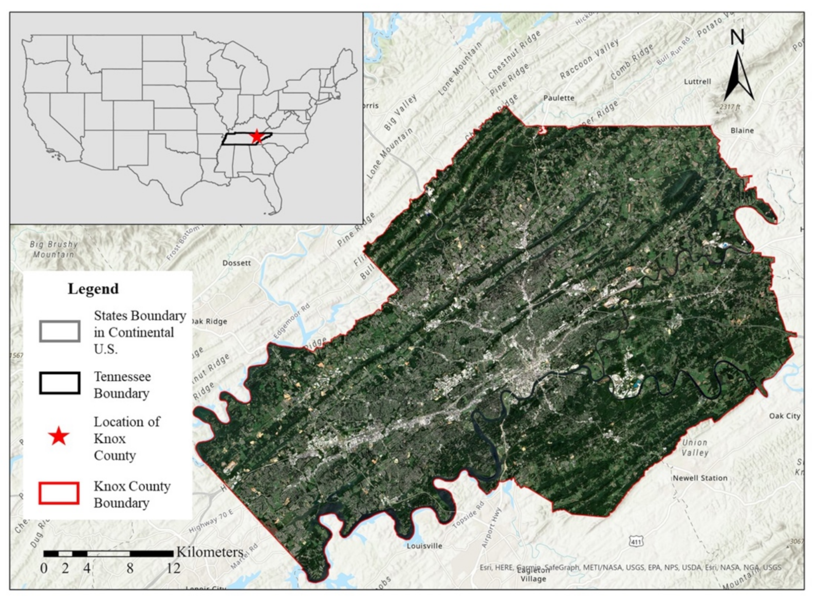
Knox County is located in Eastern Tennessee (Figure 1), covering 1316 km2 and with a population of 470,313 [21]. This area includes a set of parallel ridges and valleys oriented from northeast to southwest [22]. This area has a humid subtropical climate. The average high temperature in July is about 31 °C and the average low temperature in January is about −2 °C [23]. The annual precipitation is about 1400 mm, occurring throughout the whole year, with no significant differences between seasons [24,25]. The warm temperature and high humidity provide a favorable environment for vegetation growth [24]. Forests and herbaceous areas cover 34.12% and 21.5% of the study area, respectively [15].
2.2. Datasets
2.2.1. Remote Sensing Images and Pre-Processing
Sentinel-2 images were used to map the kudzu distribution. The Sentinel-2 satellites were launched in 2015 with multispectral instrument (MSI) sensors on board. Sentinel-2 images are freely available and frequently revisited and show improved spatial resolution, large coverage, and rich spectral information from the visible (VIS) and near-infrared (NIR) to the short-wave infrared (SWIR) bands, which is necessary for the optimal detection and mapping of invasive plants [26]. Sentinel-2 images also provide bands with narrow band widths at the red edge and near-infrared wavelengths that are sensitive to vegetation variations. Table 1 lists the main technical specifications of the Sentinel-2 image bands.
We downloaded the Level-2A products that are organized as atmospherically and geometrically corrected bottom-of-atmosphere (BOA) reflectance images (https://scihub.copernicus.eu, accessed on 12 January 2021). The Level-2A products are composed of 100 km2 tiles in UTM/WGS84 projection. Our study area is fully covered by two adjacent Sentinel-2 tiles (tile numbers 16SGF and 16SGE). Images acquired at two times were used based on the kudzu phenology—one acquired in spring (9 May 2020) when kudzu leaves had not sprouted and the other in fall (6 September 2020) when kudzu leaves are still green but defoliation of the other vegetation has not started. Both images were clear and cloud-free across the study area. Kudzu leaves grow in spring and drop in fall, with a lagging growth period compared with the surrounding vegetation. Given these unique phenological characteristics, the growth conditions derived from these two times were used to identify kudzu from other vegetation.
We extracted the images of Knox County using a shapefile boundary and resampled the bands with 20 m spatial resolution to 10 m resolution. Ten VIS (bands 2–4), red edge (bands 5–7), NIR (bands 8, 8b), and SWIR (bands 11,12) bands were composited to a multiband image stack for kudzu classification. Vegetated areas were extracted based on the classification map provided in the Sentinel-2 Level-2A products. The above image analyses were performed on ENVI 5.5.3 software.
2.2.2. Reference Data
The reference data were collected from high-resolution imagery in Google Earth. Google Earth provides a three-dimensional interactive view of the entire study area. It makes data collection more efficient without any access constraints [28]. The high-resolution imagery in Google Earth includes Geo-eye and WorldView imagery up to 0.31 m in resolution. We identified several regions that were fully invaded by kudzu and digitized the boundaries of kudzu patches in Google Earth. The other vegetation was generally categorized as trees and grasslands. Patches of typical trees and grasslands in the study area were also digitized for spectral unmixing analysis. We considered other land covers that were potentially mixed with kudzu and collected the corresponding patches in Google Earth. These patches, categorized as “others”, were mainly non-vegetated areas near kudzu invasion sites, since kudzu usually invade along the forest edges near roads and residential areas, meaning there may be some non-vegetated areas omitted from vegetation extraction. Therefore, the reference data were collected in four categories: kudzu, trees, grasslands, and others.
Kudzu is known to have a lagging growth period with a late leaf dropping stage, which makes it more distinguishable in fall. We, therefore, collected the reference data in fall, when kudzu is green and detectable. We also double checked the boundaries on the Sentinel-2 images to make sure pixels within the reference areas were fully covered by kudzu. A total of 467 polygons of kudzu, trees, grasslands, and others were digitized in Google Earth (KMZ files) in our study area. The digitized polygons were converted to shapefiles and georeferenced to the Sentinel-2 images in ArcGIS Pro 2.6.0. The digitized dataset included 237 polygons (1788 pixels) of kudzu, 45 polygons (14,588 pixels) of trees, 82 polygons (9718 pixels) of grasslands, and 103 polygons (4755 pixels) of others. These polygons were used as the reference data for unmixing spectra extraction and classification accuracy assessment.
2.3. Spectral Unmixing and Phenology-Based Kudzu Identification Method
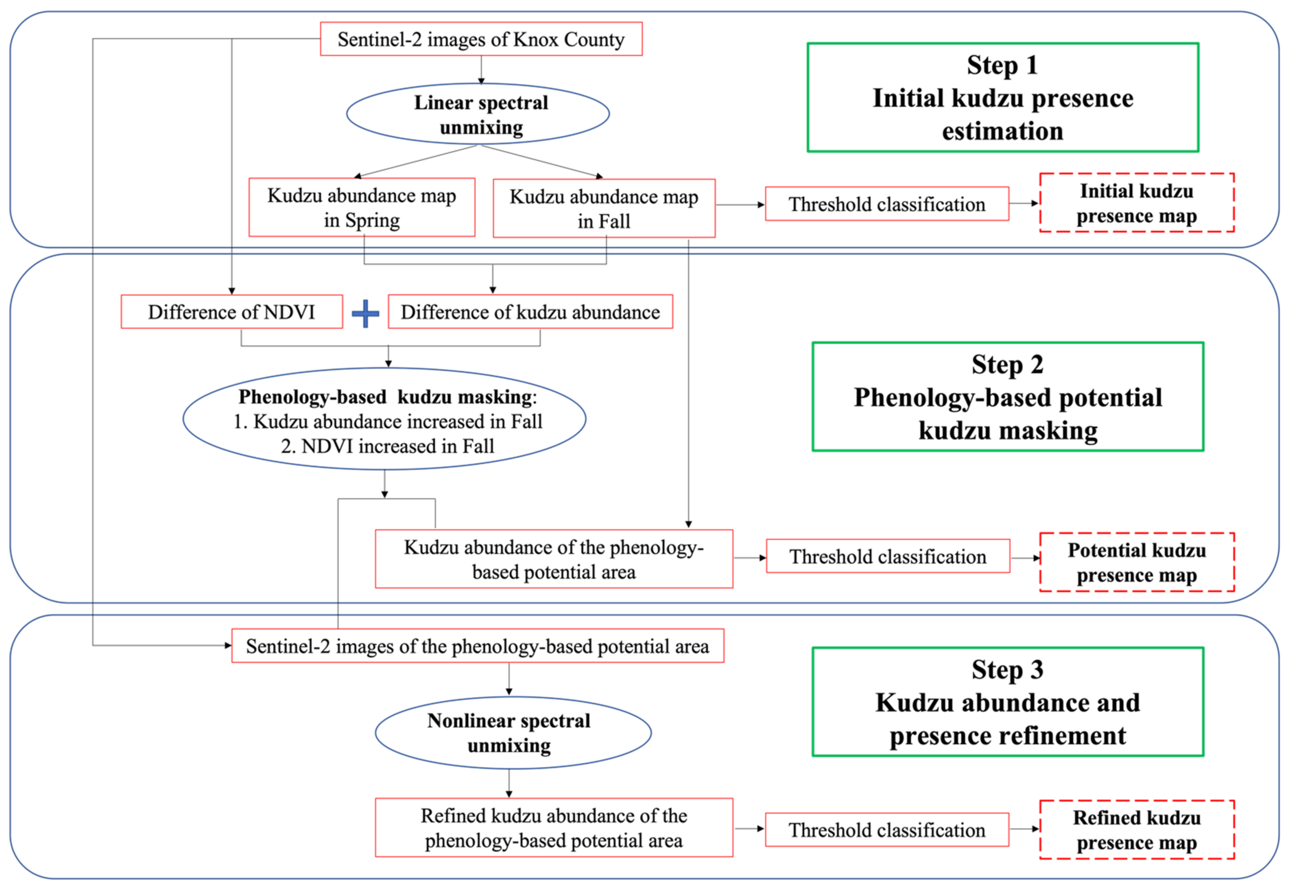
Our proposed spectral unmixing and phenology-based kudzu identification method consisted of three sequential steps (Figure 2). First, we used the linear unmixing algorithm to estimate the subpixel abundance of kudzu and the surrounding land features. Then, we integrated the phenological characteristics of kudzu with the initial linear abundance estimation to remove misclassified vegetation and to reduce the space domain for further processes. Finally, we applied the appropriate nonlinear unmixing model on the extracted areas to improve the accuracy of the kudzu presence map. The kudzu distribution was mapped using the fall image due to its high greenness at that time.
2.3.1. Initial Estimation by Linear Unmixing
As mentioned earlier, kudzu pixels in the multispectral images are mainly mixed pixels of kudzu and native plants. Spectral unmixing approaches have been developed to estimate the fractional coverage (abundance) of each feature (endmember) in a pixel [29]. The linear spectral unmixing method only considers the direct reflectance from each endmember [30]. It is easy to interpret and has been successfully applied to classify invasive plants [1,31,32].
We first applied the linear unmixing approach on the Sentinel-2 images to estimate the initial abundance. Linear spectral unmixing assumes that the observed spectrum in a pixel on the remote sensing images is the linear combination of the spectra of limited endmembers [33]. The linear coefficient of each endmember represents its abundance, corresponding to its respective areal proportions within a pixel [19]. The fully constrained least squares (FCLS) method is one of the most widely used linear unmixing approaches in urban areas [30]. In the FCLS model, the reflectance of a pixel is assumed to consist of the linear combination of endmembers and noises:
where is the pixel’s reflectance with spectral bands, is the number of endmembers, is the coefficient representing the abundance of th endmember in the pixel, is the reflectance of pure th endmember, and is the noise caused by the sensor and modeling errors. Two constraints are used in this model to derive endmember abundances, namely the abundance nonnegativity constraint (ANC) and abundance sum-to-one constraint (ASC). The ANC constraint requires that all derived endmember abundances are positive or zero values because it is impossible to have a negative presence of any endmember in the field of view of a pixel [33]. The ASC constraint requires the sum of the abundances from all endmembers to equal one [33].
2.3.2. Phenology-Based Potential Kudzu Masking
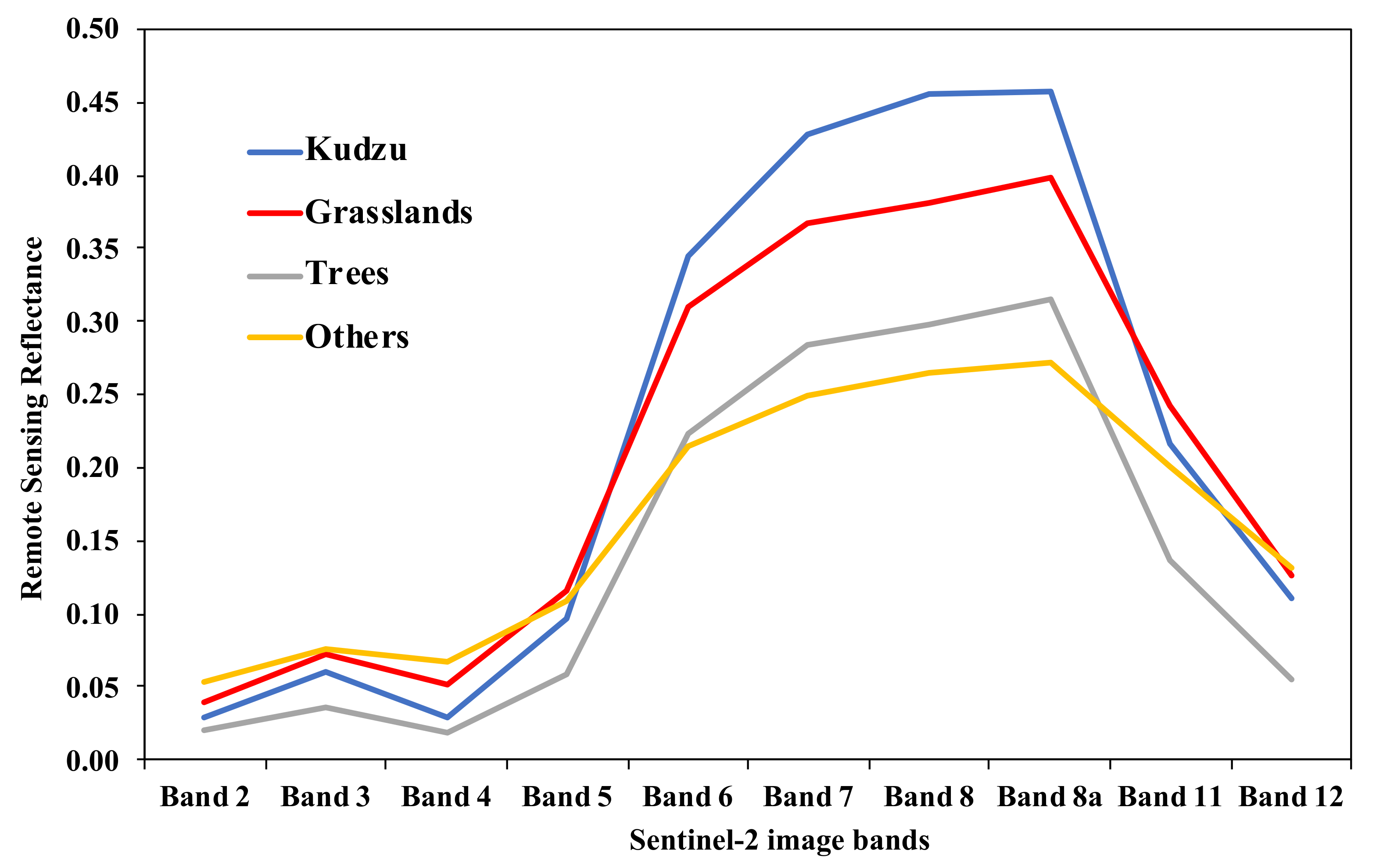
As a type of vegetation, kudzu has similar spectra with nearby trees and grasslands. Therefore, spectral information alone is not enough to accurately separate kudzu from surrounding vegetation. Figure 3 illustrates the averaged spectra of the reference areas extracted from the Sentinel-2 images. This figure suggests that kudzu, trees, and grasslands demonstrate identical shapes of the spectra curves and similar reflectance values. It is especially difficult to separate kudu and grasslands in visible (bands 2–4) and short-wave infrared (bands 11, 12) bands. Kudzu, trees, and grasslands are more spectrally separable at red edges to near-infrared bands (bands 6–8a). Therefore, it is difficult to separate kudzu from the surrounding vegetation using spectral information only.
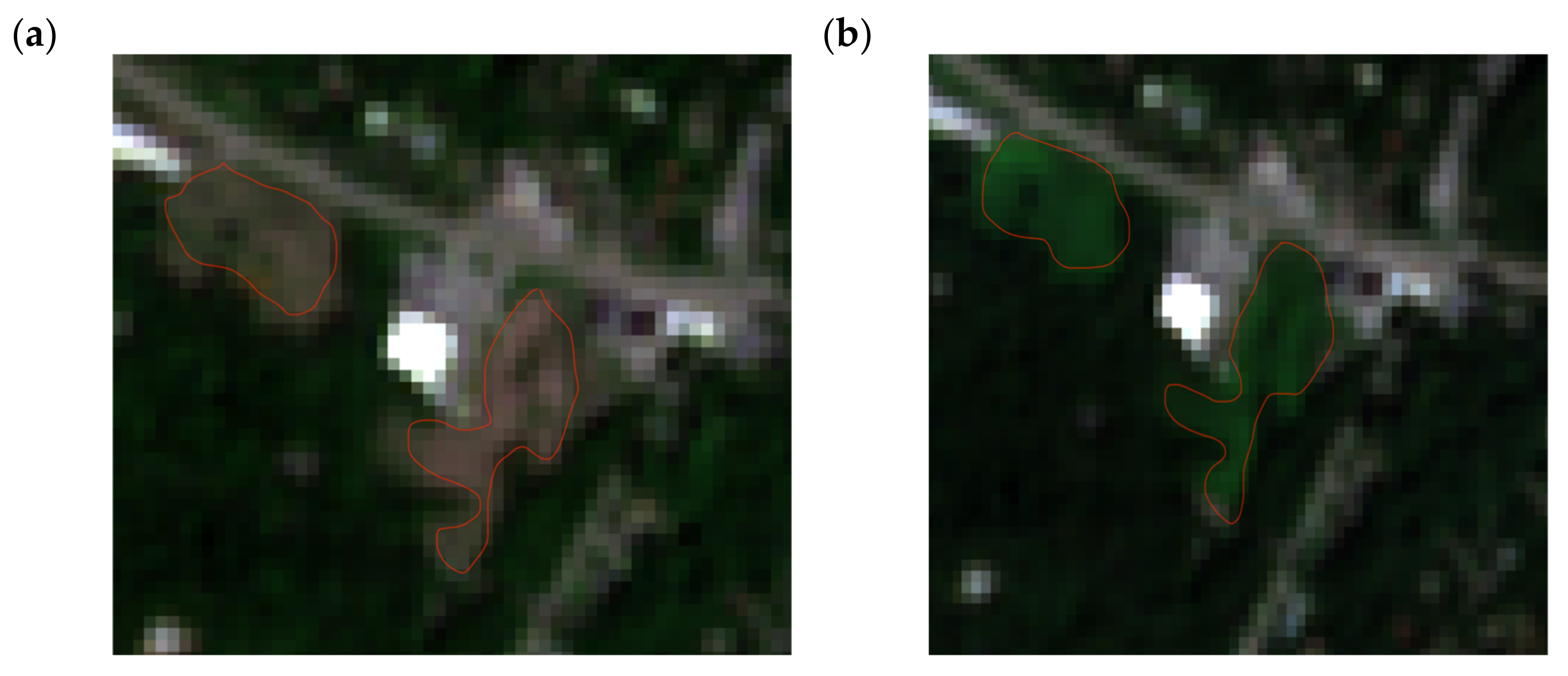
Fortunately, kudzu has a different phenology from the native plants. Kudzu leaves start to sprout late in spring [15] and remain green until the first frost, making it more distinguishable from other vegetation in the fall and early winter [34]. This unique lagging growth is one of the crucial attributes used to distinguish kudzu from the surrounding vegetation [15,17,34]. For example, kudzu had not sprouted in the spring image in this study area but the surrounding vegetation had already sprouted and their leaves can be detected in the image (Figure 4a). In the fall image, kudzu and the surrounding vegetation are all green and detectable (Figure 4b).
We applied two phenology-based rules to improve the kudzu identification. The first assumption was that the abundance of kudzu increases from spring to fall because kudzu is more detectable in the fall image. This rule was implemented by calculating the difference between the initial kudzu abundances estimated by linear unmixing in early spring and late fall. We, therefore, compared the kudzu abundance maps of the spring and fall images that were derived from the first step to extract the potential kudzu pixels.
The second assumption was that the greenness of kudzu was higher in the late fall image than the early spring image, whereas the greenness of other vegetation was higher in early spring than late fall. We used the normalized difference vegetation index (NDVI) to measure the greenness of the vegetation [35]. NDVI is defined as:
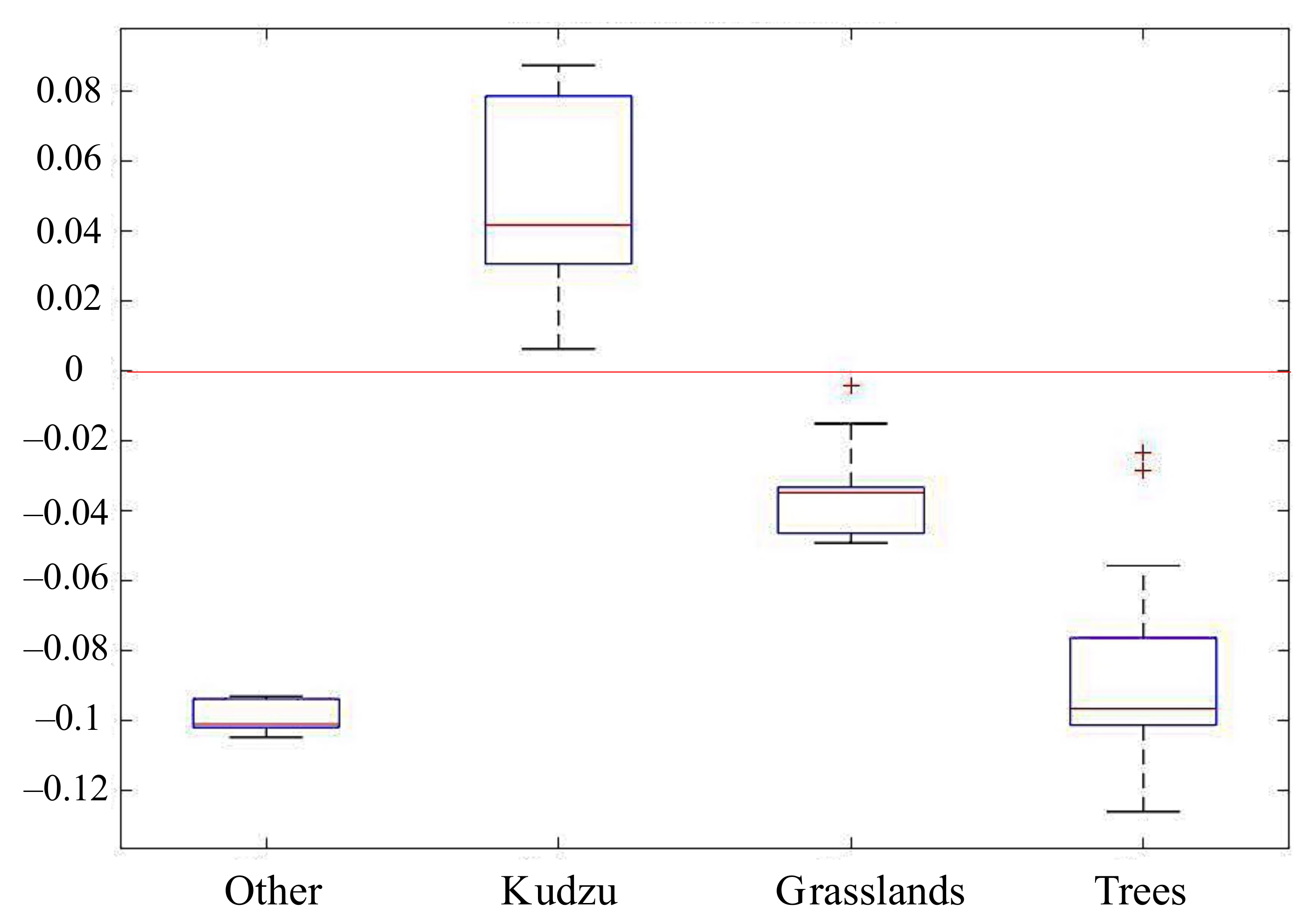
where is reflectance in the near-infrared band and is reflectance in the red band. We used band 8 and band 4 of the Sentinel-2 images for and , respectively. High NDVI values correspond to more vegetation cover based on their dependency [36]. Figure 5 illustrates the NDVI variations of kudzu and the surrounding vegetation on the spring and fall images in the reference regions. The NDVI changes in kudzu reference regions were all positive. In contrast, the NDVI changes from the other three categories were negative, consistent with our assumptions.
Based on the above two assumptions, we created a kudzu mask based on the differences in kudzu abundance and NDVI values. Specifically, the pixels where both NDVI and kudzu abundance increased from spring to fall were marked as kudzu pixels. This kudzu mask can be used to remove misclassified kudzu pixels and reduce the domain for further processes.
2.3.3. Nonlinear Unmixing Refinement
Kudzu usually grows on top of the native trees, causing multilayer scattering and uneven contributions of kudzu and surrounding vegetation to a pixel’s reflectance. The linear unmixing model we used in the first step does not consider the indirect reflectance from the interaction among endmembers within a pixel, limiting the accuracy of the produced abundance map [29]. Unlike the linear unmixing models, nonlinear unmixing models are designed for complex reflectance surfaces with multi-scattering. They are especially effective for heterogeneous landscapes consisting of small patches, which is a more precise description of the kudzu surfaces. However, the nonlinear unmixing models are usually computationally intensive and are not efficient for regional analysis [37]. We, therefore, only applied the nonlinear unmixing models on the pixels that were extracted using the previous steps to refine the kudzu abundance map at a low computation cost.
Another issue is identifying which nonlinear model is suitable for kudzu mapping, because multiple nonlinear unmixing models exist but no study has been conducted to examine the performance of these models for kudzu mapping. We evaluated five nonlinear models, including the bilinear fan model (BFM), post-polynomial nonlinear model (PPNM), Hapke-based model (HM), generalized bilinear model (GBM), and multi-harmonic post-nonlinear mixing model (MHPNMM). These nonlinear models were developed for different reflectance scenarios and radiant transmission assumptions. BFM and GBM are bilinear models that assume a light ray would interact with two different endmembers before reaching the sensor, while GBM offers more degrees of freedom than BFM [38]. The physical assumption of BFM and GBM is that the probability of nonlinear interactions between endmembers is governed by their abundance. PPNM improves the unmixing process by including the self-interaction between endmembers [39]. HM is designed for intimate mixtures where lights interact multiple times with the closely contacted particles on the ground before reaching the sensor [40]. MHPNMM combines the characteristics of PPNM, GBM, and HM to simulate the high-order interactions between endmembers [41]. Detailed descriptions of these models can be found in [38,39,40,41]. We compared the performances of these nonlinear models and selected the most suitable model for the kudzu mapping.
2.3.4. Creating Kudzu Presence Maps
A kudzu presence map is created in each step via endmember abundance estimation and threshold reclassification. Endmember abundances are estimated via spectral unmixing analysis. We defined four land cover features as endmembers: kudzu, trees, grasslands, and others. We adopted the four-endmember strategy for spectral unmixing analysis due to their distinct spectral signatures compared to a binary strategy involving kudzu and non-kudzu classes, making the abundance estimation more accurate. The four endmembers were also consistent with the four categories of reference data. Pixels within the reference polygons were assumed to be pure pixels. The spectral library used in spectral unmixing analysis contained the average reflectance of the pure pixels extracted from the reference regions in the fall image. This spectral library was used for both linear unmixing and nonlinear unmixing analyses. Abundance maps were produced for kudzu, trees, grasslands, and others in the spectral unmixing analysis.
The threshold continuum reclassification was applied to the abundance maps to create the classification maps. This approach was designed to discretize the abundance of invasive plants by characterizing the landscape based on the magnitude of invasion [1]. Specifically, all pixels with abundance values greater than or equal to the threshold value were aggregated as ‘presence’, whereas the pixels with abundance values lower than the threshold were aggregated as ‘absence’ for each endmember. In this way, the landscape was treated with a gradually changing gradient and isolated pixels and patches were eliminated [1]. We tested 10 thresholds from 0.1 to 1.0 in each step and used the optimal threshold to create the kudzu presence maps.
2.4. Accuracy Assessment
We regrouped the classification into two categories: kudzu and non-kudzu (includes trees, grasslands, and others), focusing mainly on the accuracy of the kudzu classification. A confusion matrix was generated to evaluate the classification accuracy of the kudzu presence maps by treating the pixels within the kudzu reference polygons as the ground truth. We also visually checked the kudzu presence maps against the reference kudzu areas to interpret the mapping quality.
We derived four indices from the confusion matrix to quantify the classification accuracy: producer’s accuracy (PA) [42], user’s accuracy (UA) [42], Jaccard index (Jaccard) [43], and Cohen’s kappa index (Kappa) [44]. PA and UA are primary accuracy measures for individual classes [42,45]. We only derived the PA and UA values for kudzu. The PA value represents the number of correctly classified kudzu pixels in the reference polygons divided by the total number of kudzu reference pixels, representing the probability that a ground kudzu pixel will be correctly classified [46]. The UA value represents the number of correctly classified kudzu pixels in the reference polygons divided by total number of pixels classified as kudzu, representing the probability that a pixel in the kudzu presence map represents kudzu on the ground [46]. PA and UA provide the omission and commission errors, respectively. The PA and UA at threshold are derived using Equations (5) and (6), respectively:
where TP (true positive) is the number of pixels identified as kudzu within kudzu reference polygons, FN (false negative) is the number of pixels identified as non-kudzu (trees, grasslands, or others) within kudzu reference polygons, and FP (false positive) is the number of pixels identified as kudzu within non-kudzu reference polygons (trees, grasslands, and others).
The Jaccard index is another accuracy measure at the category level. Unlike PA and UA, the Jaccard index compares the true positive with both false negative and false positive predictions. The Jaccard index ranges from 0 to 1 and the maximum occurs when there are only true kudzu presence predictions and no errors [43]. The Jaccard is derived using the Equation (7) for each threshold i:
Cohen’s kappa index is a widely used accuracy measure for the entire classification process, showing the proportion of agreement after chance agreement is removed [44]. It is derived with consideration of both commission and omission errors for all categories [46]. The Kappa at threshold is derived using Equations (8)–(10):
where TN (true negative) is the number of pixels identified as non-kudzu within non-kudzu reference polygons (trees, grasslands, and others).
We used the Kappa to evaluate the classification performances on both kudzu and non-kudzu categories because it assesses the robustness of the classification in identifying the non-kudzu areas, reducing potential misclassifications caused by insufficient kudzu reference data. The Kappa values range from 0 to 1, where 1 indicates perfect agreement for all categories and 0 indicates random agreement [46,47]. We interpreted the Kappa index according to Cohen’s suggestion: 0–0.20 as none to slight agreement with the reference data; 0.21–0.40 as fair; 0.41–0.60 as moderate; 0.61–0.80 as substantial; 0.81–1.00 as almost perfect agreement [47].
3. Results
3.1. Performance of the Initial Linear Unmixing Estimation for Kudzu Mapping
We evaluated the accuracy of kudzu classification maps based on abundance derived from the linear unmixing method (the first step). Table 2 lists the accuracy measures for kudzu classification based on the reclassification of different thresholds. All four indices indicate that the accuracy of the kudzu classification decreased with decreasing thresholds. This is because lower reclassification thresholds of kudzu abundance indicate that pixels with higher abundances of other endmembers are classified as kudzu presence, causing more misclassification. The PA and UA values decreased from 0.989 to 0.616 and from 0.511 to 0.152, respectively, for the thresholds from 1.0 to 0.1. Note that the PA value was much higher than the UA value for each threshold, indicating that although most kudzu in the reference areas were classified as kudzu, many surrounding vegetation areas were misclassified as kudzu. The Jaccard and Kappa index values also decreased from <0.6 to <0.2 with the decreasing thresholds. The Jaccard values imply that less than half of kudzu presence predictions were correct (true positive), regardless of the selection of threshold values. The Kappa values show that the classified kudzu and non-kudzu maps only had moderate to fair agreement with the reference data. Visual interpretation of the classification maps suggests that most misclassifications of kudzu were from grasslands.
In summary, the kudzu reference areas were well identified by the linear unmixing method, although many grassland areas were also misclassified as kudzu. The kudzu maps created using the linear unmixing method overestimated the kudzu presence in the study area.
3.2. Performance of Phenology-Based Kudzu Masking
Table 3 lists the accuracy indices of the kudzu classification maps after applying the phenology-based kudzu mask. The PA, UA, and Jaccard values show similar decreasing trends with decreasing thresholds, although all values are higher than those in the first step, especially for the UA and Jaccard values. The PA values are still high, decreasing from 1 to 0.687 for thresholds ranging from 1.0 to 0.1. The UA values are improved by approximately 0.3 compared to the values in the first step, decreasing from 0.802 to 0.506 for thresholds ranging from 1.0 to 0.1. The Jaccard values are also elevated to 0.802–0.411 for thresholds ranging from 1.0 to 0.1, indicating that >50% of kudzu presence predictions were correct for thresholds of >0.3. The improvement of the UA and Jaccard values indicate that the use of the phenology-based mask can significantly reduce the kudzu misclassification in the first step. Visual interpretation also shows that most misclassified grasslands in the first step were excluded after the phenology-based masking.
The Kappa index behaves differently in this step, first increasing then decreasing with decreasing thresholds. The highest Kappa value, 0.525, occurs at the threshold of 0.6. The high PA, UA, and Jaccard values for the kudzu class but low Kappa values for both classes at thresholds ≥ 0.7 suggest that the reclassified maps at thresholds ≥ 0.7 have high accuracy for kudzu presence but poor accuracy for the non-kudzu presence. This resulted from the bias of the high true positive (kudzu reference samples) values but low true negative (non-kudzu reference samples) values in the confusion matrix of high thresholds, because most pixels with high abundance of non-kudzu categories were excluded from the phenology-based masking.
3.3. Performance of the Nonlinear Unmixing Refinements for Kudzu Mapping
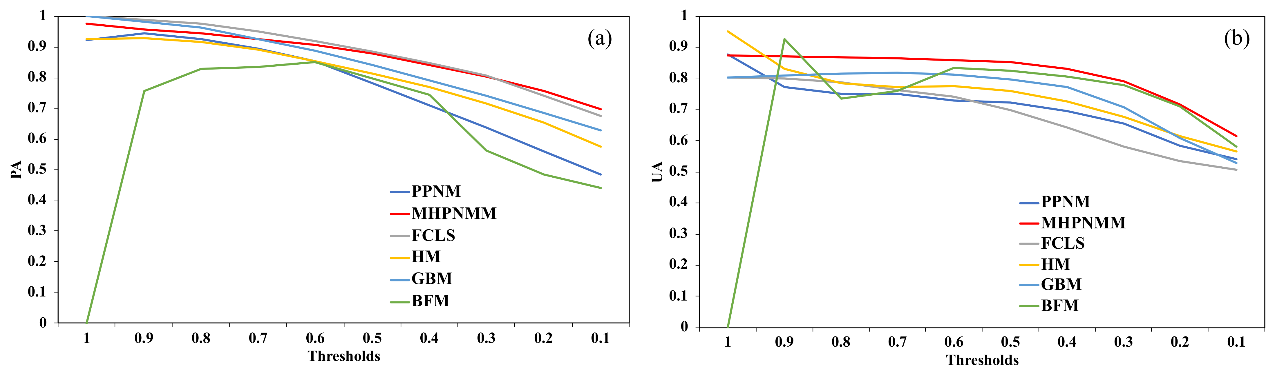
As listed in Table 4, only 12% of the study area was used for the nonlinear unmixing analysis (134 km2 out of 1126 km2). The performances of the five nonlinear unmixing models, namely BFM, GBM, PPNM, HM, and MHPNMM, and the linear unmixing model used in the first step, FCLS, were assessed for kudzu classification using the UA and PA values (Figure 6). The PA and UA values for kudzu decreased with the decreasing thresholds for all nonlinear unmixing models except BFM. FCLS, GBM, and MHPNMM provided relatively higher PA values, with MHPNMM providing the highest UA values. We, therefore, selected MHPNMM to estimate the nonlinear abundance and to refine the kudzu presence maps.
Table 5 lists the classification accuracy indices based on the nonlinear model, MHPNMM. Both PA and UA values are higher than 0.8 and the Jaccard values are higher than 0.7 at thresholds ≥ 0.4, suggesting that both commission and omission errors are <20% for kudzu classification, while correctly classified kudzu areas account for >70% of all predictions. The Kappa results show similar trends (first increasing then decreasing) to the results of the second step. The highest Kappa value, 0.725, occurs at the threshold of 0.6, indicating that the overall classification is in compliance with the reference data for both kudzu and non-kudzu samples.
3.4. Kudzu Presence in Knox County
We selected an optimal threshold to create the kudzu presence maps. The highest PA, UA, and Jaccard values for kudzu classification occurred at a threshold of 1.0, although the corresponding Kappa value was low, indicating that the overall classification was not robust, especially for the non-kudzu vegetation. The highest Kappa values occurred at the threshold of 0.6 in step 2 and step 3, while the corresponding PA, UA, and Jaccard values were also high, indicating more robust classification for both kudzu and non-kudzu classes. We, therefore, used 0.6 as the optimal threshold to create the kudzu presence maps for all steps.
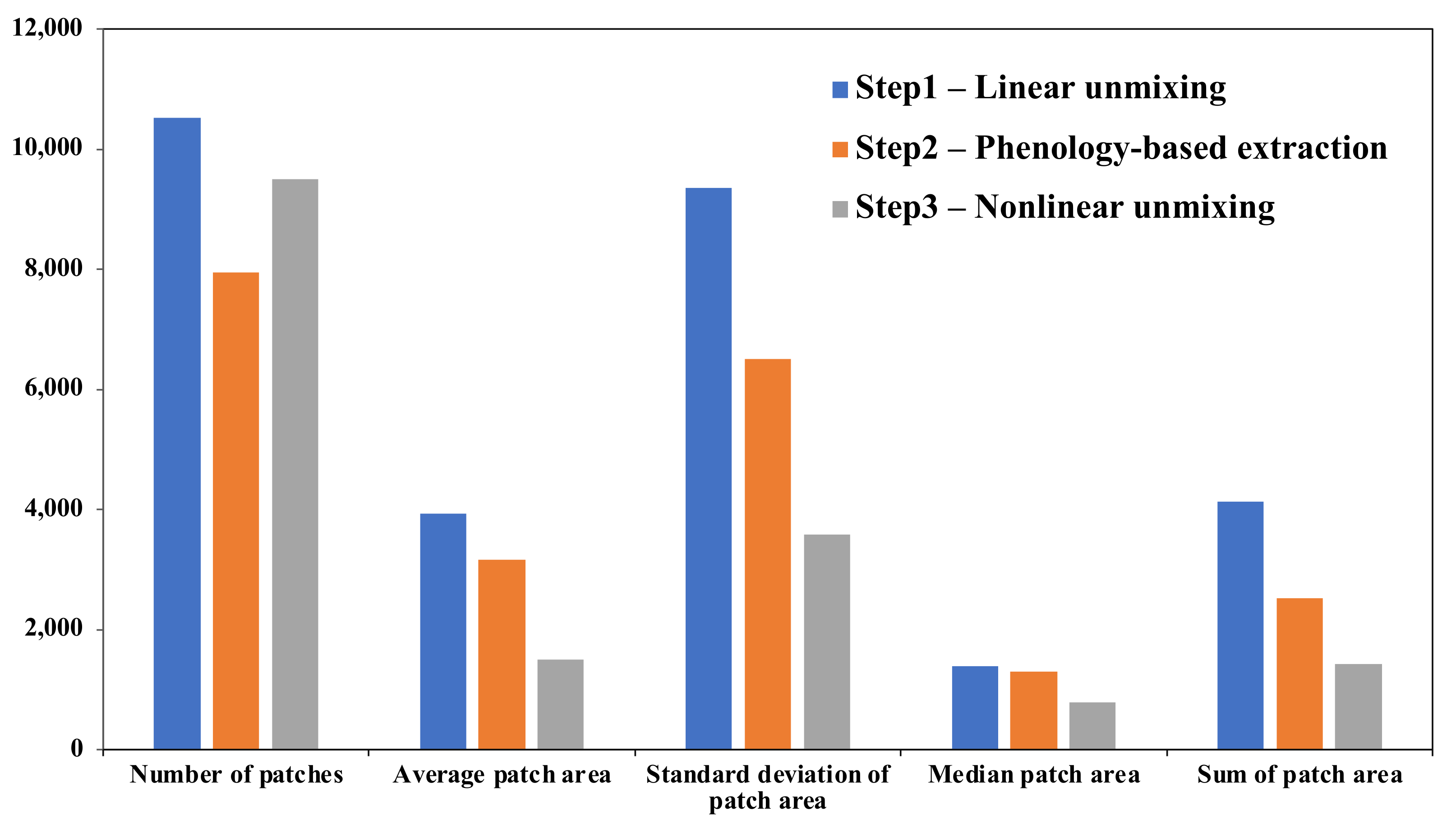
Figure 7 illustrates the statistics for the kudzu patches identified in the kudzu presence maps. The initial kudzu presence map from the first step produced the highest number of kudzu patches, covering the largest areas, with high standard deviation in some areas. In the second step, the phenology-based masking reduced the number of kudzu patches, the patch area, and the standard deviation of the area slightly, although the total kudzu area decreased by >50% from the first step. In the third step, the nonlinear unmixing models further reduced the kudzu patch area, standard deviation, and total kudzu area by about 50% from the second step, although the number of kudzu patches increased. These results confirmed that the linear unmixing model tends to overpredict kudzu presence, the phenology-based masking reduces the total area of kudzu patches, and the nonlinear unmixing model predicts more kudzu patches with a smaller area and less variation.
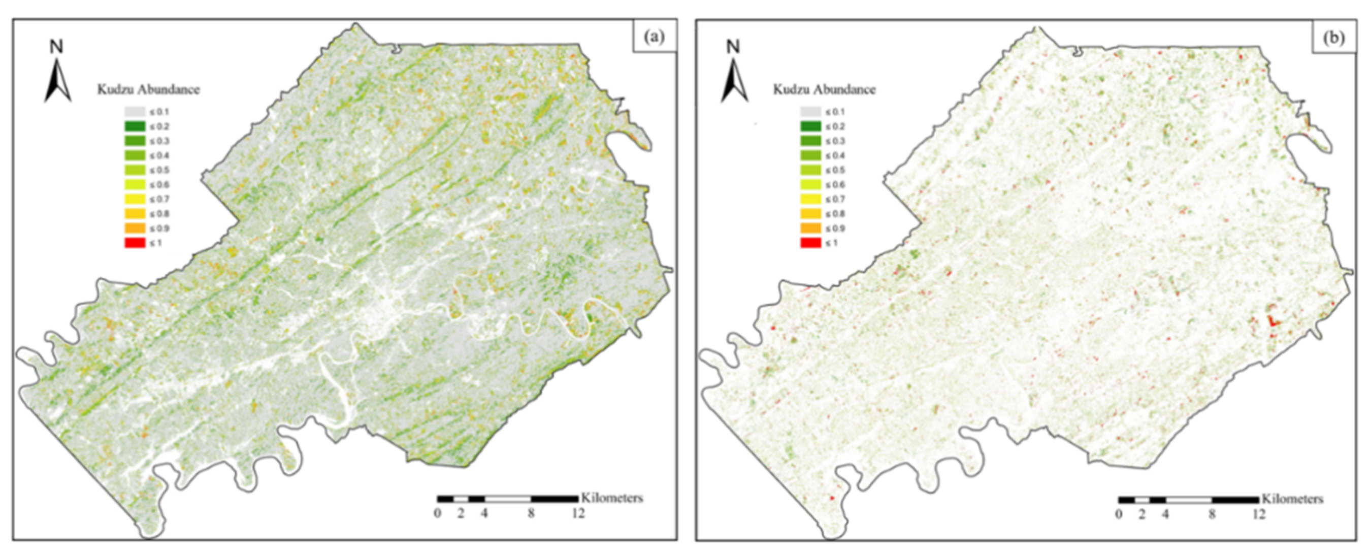
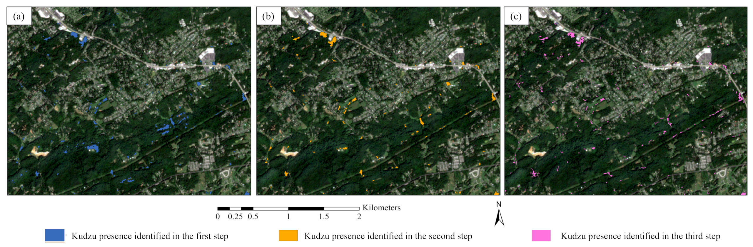
The kudzu abundance maps estimated from linear and nonlinear unmixing are shown in Figure 8. Areas with high kudzu abundance are sporadically distributed across the entire county. The northwestern and southeastern parts in Knox County are heavily invaded by kudzu. The identified kudzu invasion areas continuously decreased from the first to the third step. The final refined kudzu presence map identified 1.05% of the vegetated areas in Knox County as kudzu, with PA, UA, Jaccard, and Kappa values of 0.907, 0.858, 0.789, and 0.725, respectively. The kudzu presence maps also suggest that kudzu usually invade forest edges, roads, and vegetation near houses and infrastructure (Figure 9).
4. Discussion
4.1. Misclassification with the Surrounding Vegetation
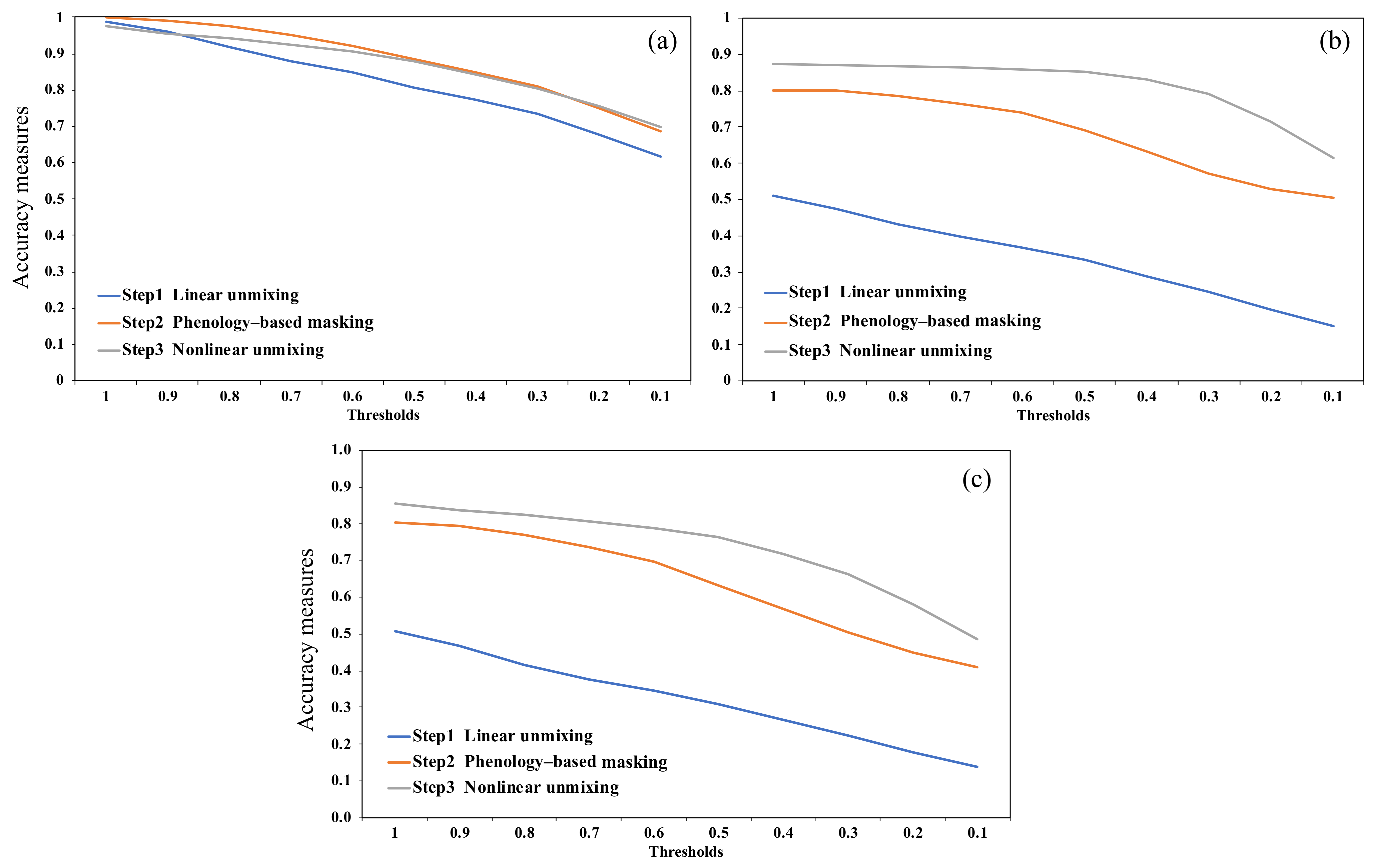
A comparison of the accuracy indices for kudzu classification indicated that the PA values were relatively constant, while the UA and Jaccard values significantly increased from the first to the third step of the classification (Figure 10). The initial linear unmixing model was capable of identifying kudzu in the reference regions, although it overpredicted the kudzu presence by misclassifying the surrounding vegetation as kudzu. The phenology-based masking and nonlinear unmixing approach reduced the misclassification and increased the UA and Jaccard values from less than 0.5 in the first step to approximately 0.9 in the third step, producing more accurate kudzu maps.
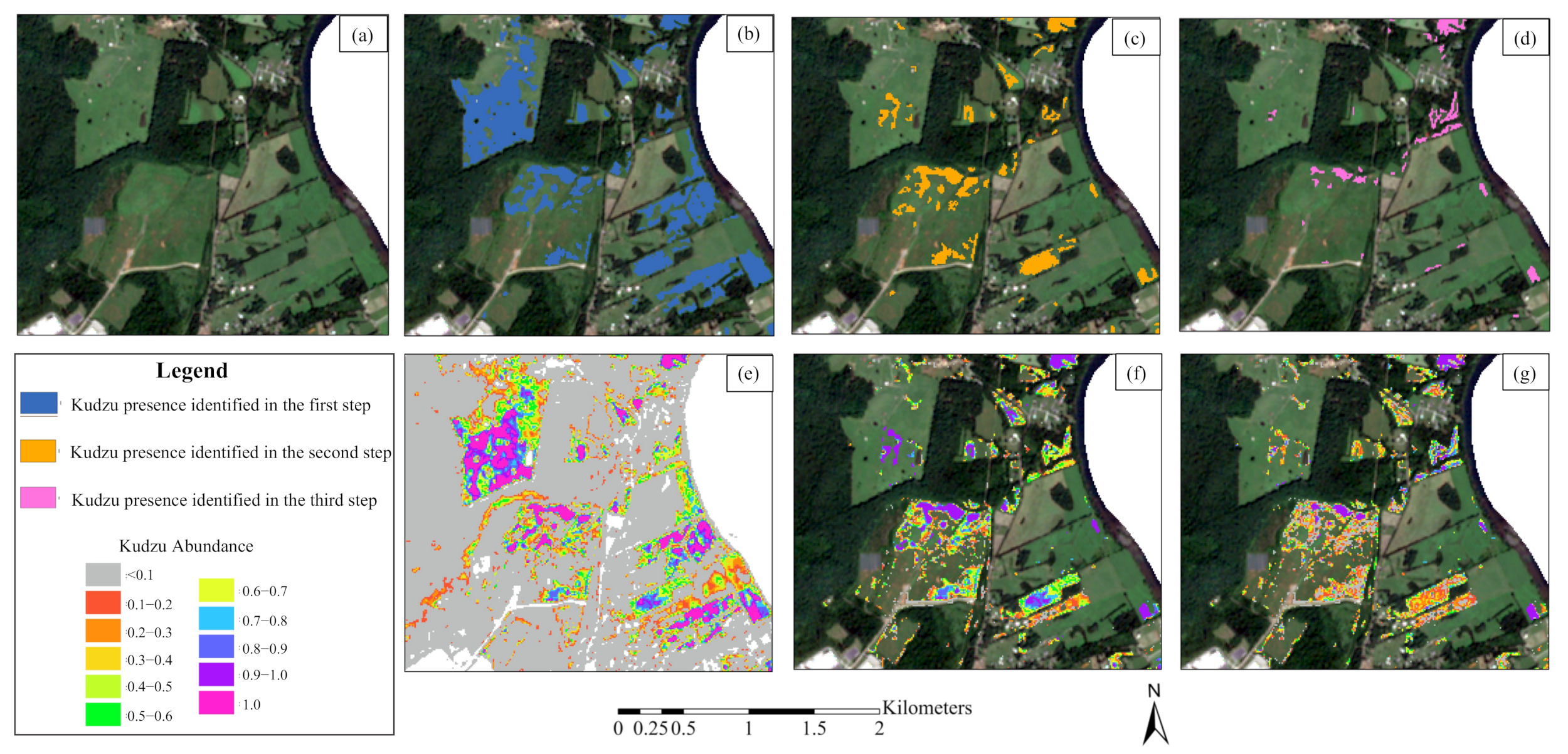
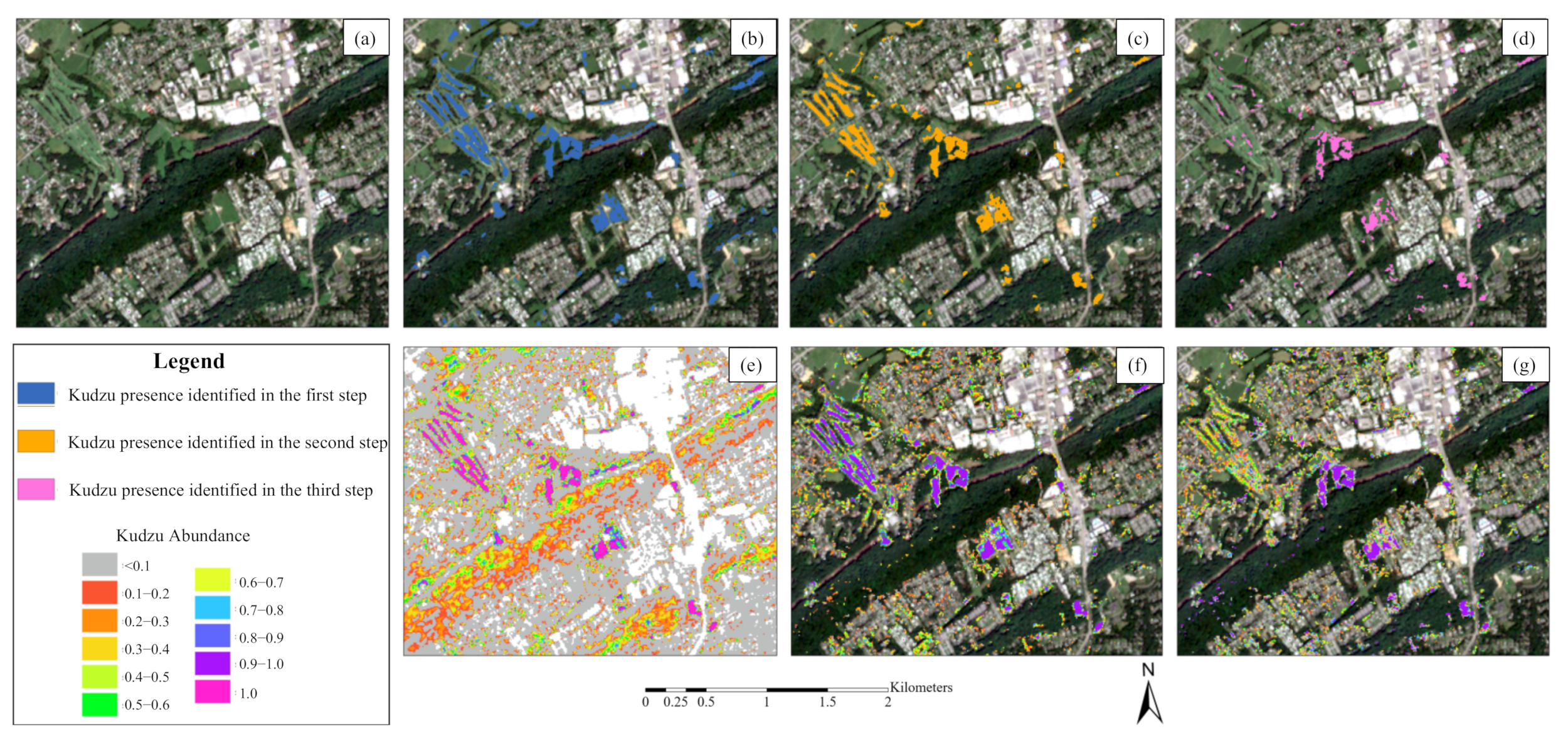
Here, kudzu was primarily misclassified as grassland. Figure 3 shows that the spectral curves for kudzu and grassland areas collected from Sentinel-2 images are very close to each other, which caused misclassification. Figure 11 and Figure 12 provide two examples. The field in Figure 11 is covered by several large patches of grassland that were misclassified as kudzu in the first step (Figure 11b,e). The phenology-based masking excluded most grasslands (Figure 11c,f). The nonlinear unmixing method further reduced the misclassification and only some edges of forests were identified as kudzu (Figure 11d,g). Figure 12 shows the residential regions with small grassland patches. The grassland stripes on the western parts were identified as kudzu in the first step, while the phenology-based masking also failed to exclude these areas (Figure 12b,c,e,f). These misclassified grasslands were excluded in the third step, and the remaining patches along the roads and houses were identified as true kudzu presence based on the validation of our reference data (Figure 12d,g).
4.2. Spectral Unmixing Model Selection for Kudzu Mapping
Spectral unmixing models are designed for specific reflectance scenarios and radiant transmission processes. Studies have found that unmixing models perform dramatically differently for various landscapes [12]. Therefore, an appropriate unmixing model for kudzu mapping and identification should demonstrate reasonable interpretation of the suitability of the modeling conditions and the invaded surfaces.
Physical interpretation of the spectral unmixing models was investigated in this study for kudzu surfaces. Linear unmixing models are intuitive and only consider the contribution of direct endmember reflectance. The linear unmixing models are, therefore, more suitable for flat surfaces that consist of spatially separated pure materials [40]. The so-called checkerboard pattern can be compromised at a large spatial scale when the influence of the local topography is minor. We, therefore, applied the linear unmixing model across the entirety of Knox County in the first step, which estimated the initial kudzu abundance and presence with small computation expense. However, the interaction of lights between vegetation endmembers in the vertical structure was highly nonlinear [37]. The nonlinear unmixing approach provides more accurate descriptions for complex spectral and geometrical scenarios [48]. Bilinear models, including BFM, GBM, and PPNM, often describe the scenes acquired over forested areas where there are many interactions between the ground and canopy [49]. Hapke-based models are valued for accurate and realistic abundance estimation in distinguishing mineral materials at small spatial scales, focusing on closely packed particles with different optical characteristics [50]. MHPNMM considers multilayer scattering and internal radiation interactions on rugged surfaces [41]. MHPNMM is more generalized and robust for various unmixing scenarios due to the combination of bilinear and Hapke-based models. The nonlinear unmixing model for kudzu classification should include both the indirect reflectance between the ground and vegetation and multiple scatters from the vertical structure of the tree canopy and kudzu leaves, since kudzu usually invades forests edges and grows on top of trees. MHPNMM represents the spectral mixing processes of kudzu surfaces properly, making it suitable for accommodating complex mixed scenes for refined kudzu classification.
4.3. Future Improvements of the Proposed Kudzu Classification Approach
Our proposed method could be further improved in terms of the spectral unmixing parameters and phenological characteristic collection. First, it can be improved by incorporating a spectral library collection. A precise spectral library of endmembers is the foundation for accurate spectral unmixing analysis and abundance estimation. We collected endmember spectra in Google Earth with the assumption that they contained “pure” pixels, which may not always be true in practice. A more precise spectral library could be obtained by collecting spectra in the field using spectrometers to capture more differences in the spectral signatures [51].
Second, an optimal combination of unmixing bands would reduce the redundant information and improve the accuracy and efficiency of spectral unmixing. We used all bands with original resolutions of 10 m and 20 m for Sentinel-2 images, including visible, red edge, NIR, and SWIR bands. Red and NIR bands are commonly regarded as the most important bands for spectral unmixing analyses in vegetated regions [52]. However, studies have found that the most important bands for Sentinel-2 images for vegetation abundance estimations are bands 4 (Red), 8 (NIR), and 12 (SWIR), while the special red edge bands (bands 5 to 7) have little influence in terms of improving the accuracy of vegetation abundance estimation due to their high correlation with other bands [53]. Kudzu mapping, therefore, can be improved by investigating the performances of different band combinations for spectral analysis and selecting the optimal combinations to diminish the noises caused by redundant bands and increase their computation efficiency.
Third, the numbers and types of endmembers also affect the performance of spectral unmixing analysis. More specific endmember types would increase the accuracy of spectral unmixing-based classification [51]. Shade was also reported to play a significant role in identifying vegetation species in spectral unmixing analyses [31]. We only considered the general categories of the surrounding vegetation, including trees, grasslands, and others. Further studies could investigate the effects of specifying native plant species and involving shade as an endmember in spectral unmixing analyses.
Finally, kudzu phenology was not fully incorporated in the current study. The characteristics of kudzu phenology can be improved by exploring kudzu greenness changes over a complete growth period and identifying the significant growth time for spectral unmixing analysis.
5. Conclusions
Spectral unmixing analysis is an effective approach to identify invasive plants, especially for multispectral remote sensing imagery with medium spatial resolutions. The integration of phenological characteristics significantly improves the classification accuracy and computational efficiency for the application of advanced nonlinear unmixing models. The use of an appropriate nonlinear unmixing model allows for more accurate abundance estimations and presence mapping. This paper introduces a three-step classification process that consists of linear unmixing, phenology-based masking, and nonlinear unmixing to identify the presence of kudzu in Knox County. The major findings of this study include:
- The spectral unmixing approach is appropriate for kudzu mapping at the county scale using Sentinel-2 images and allows for continuous monitoring of large areas;
- Linear unmixing provides high producer’s accuracy but low user’s accuracy due to the misclassification of grasslands as kudzu;
- A phenology-based mask can be created based on the differences of kudzu abundance estimated from linear spectral unmixing and NDVI derived from the Sentinel-2 images. The use of this phenology-based mask improves the kudzu classification accuracy and decreases the computing expense for nonlinear spectral unmixing;
- The nonlinear unmixing analysis can refine the kudzu abundance estimation and presence classification, although an appropriate nonlinear model should be selected based on the performance assessment on the datasets and the physical interpretation of the spectral mixing scenarios;
- The refined kudzu presence map for Knox County gives user’s accuracy, producer’s accuracy, Jaccard index, and Kappa index values of 0.858, 0.907, 0.789, and 0.725, respectively, based on an optimal abundance reclassification threshold of 0.6;
- Kudzu plants are scattered in small patches along forest edges, roads, and vegetation tops near houses and infrastructure, especially in the northwestern and southeastern parts of Knox County.
The classification method introduced in this paper can be used to map kudzu in other areas. It can be applied to other invasive plants for long-term and large-scale monitoring using the free Sentinel-2 imagery.
Author Contributions
M.S. and M.T. designed the method and experiments and performed data processing and analysis. M.S. wrote the original manuscript. Y.L. and M.T. revised the manuscript. Y.L. conducted the project administration and funding acquisition. All authors have read and agreed to the published version of the manuscript.
Funding
Funding for open access to this research was provided by the University of Tennessee’s Open Publishing Support Fund.
Institutional Review Board Statement
Not applicable.
Informed Consent Statement
Not applicable.
Data Availability Statement
The Sentinel-2 imagery can be downloaded from: https://scihub.copernicus.eu/dhus/#/home, accessed on 12 January 2021). The reference data presented in this study are available on request from the authors.
Acknowledgments
The Sentinel-2 images are provided by the European Space Agency Copernicus Open Access Hub. The authors thank Nathan McKinney and Wanwan Liang from the University of Tennessee for sharing valuable kudzu data. We are grateful to the three anonymous reviewers who provided helpful comments and suggestions to improve the manuscript.
Conflicts of Interest
The authors declare no conflict of interest.
References
- Frazier, A.; Wang, L. Characterizing spatial patterns of invasive species using sub–pixel classifications. Remote Sens. Environ. 2011, 115, 1997–2007. [Google Scholar] [CrossRef]
- Gavier-Pizarro, G.I.; Kuemmerle, T.; Hoyos, L.E.; Stewart, S.I.; Huebner, C.D.; Keuler, N.S.; Radeloff, V.C. Monitoring the invasion of an exotic tree (Ligustrum lucidum) from 1983 to 2006 with Landsat TM/ETM+ satellite data and Support Vector Machines in Córdoba, Argentina. Remote Sens. Environ. 2012, 122, 134–145. [Google Scholar] [CrossRef] [Green Version]
- Hawthorne, T.; Elmore, V.; Strong, A.; Bennett-Martin, P.; Finnie, J.; Parkman, J.; Harris, T.; Singh, J.; Edwards, L.; Reed, J. Mapping non–native invasive species and accessibility in an urban forest: A case study of participatory mapping and citizen science in Atlanta, Georgia. Appl. Geogr. 2015, 56, 187–198. [Google Scholar] [CrossRef]
- Mackay, A. Climate change 2007: Impacts, adaptation and vulnerability. Contribution of Working Group II to the fourth assessment report of the Intergovernmental Panel on Climate Change. J. Environ. Qual. 2008, 37, 2407. [Google Scholar] [CrossRef]
- Beck, K.G.; Zimmerman, K.; Schardt, J.D.; Stone, J.; Lukens, R.R.; Reichard, S.; Randall, J.; Cangelosi, A.A.; Cooper, D.; Thompson, J.P. Invasive species defined in a policy context: Recommendations from the Federal Invasive Species Advisory Committee. Invasive Plant Sci. Manag. 2008, 1, 414–421. [Google Scholar] [CrossRef]
- Norambuena, H.; Escobar, S. Control biologico del espinillo en Chiloe. Tierra Adentro 2007, 77, 50–52. [Google Scholar]
- Tamura, M.; Tharayil, N. Plant litter chemistry and microbial priming regulate the accrual, composition and stability of soil carbon in invaded ecosystems. New Phytol. 2014, 203, 110–124. [Google Scholar] [CrossRef] [PubMed]
- Lehmann, J.R.; Prinz, T.; Ziller, S.R.; Thiele, J.; Heringer, G.; Meira-Neto, J.A.; Buttschardt, T.K. Open–source processing and analysis of aerial imagery acquired with a low–cost unmanned aerial system to support invasive plant management. Front. Environ. Sci. 2017, 5, 44. [Google Scholar] [CrossRef] [Green Version]
- Müllerová, J.; Brůna, J.; Bartaloš, T.; Dvořák, P.; Vítková, M.; Pyšek, P. Timing is important: Unmanned aircraft vs. satellite imagery in plant invasion monitoring. Front. Plant Sci. 2017, 8, 887. [Google Scholar] [CrossRef] [Green Version]
- Bradley, B.A. Remote detection of invasive plants: A review of spectral, textural and phenological approaches. Biol. Invasions 2014, 16, 1411–1425. [Google Scholar] [CrossRef]
- Xun, L.; Wang, L. An object–based SVM method incorporating optimal segmentation scale estimation using Bhattacharyya Distance for mapping salt cedar (Tamarisk spp.) with QuickBird imagery. GISci. Remote Sens. 2015, 52, 257–273. [Google Scholar] [CrossRef]
- Ji, W.; Wang, L. Phenology–guided saltcedar (Tamarix spp.) mapping using Landsat TM images in western US. Remote Sens. Environ. 2016, 173, 29–38. [Google Scholar] [CrossRef]
- Alderman, D.H. Channing Cope and the making of a miracle vine. Geogr. Rev. 2004, 94, 157–177. [Google Scholar] [CrossRef]
- Gerald, E.W.; Brendon, M.H.; Kudzu Vine, L. Pueraria montana, Adventive in Southern Ontario. Can. Field-Naturalist 2012, 126, 31–33. [Google Scholar] [CrossRef] [Green Version]
- Liang, W.; Abidi, M.; Carrasco, L.; McNelis, J.; Tran, L.; Li, Y.; Grant, J. Mapping vegetation at species level with high–resolution multispectral and lidar data over a large spatial area: A case study with Kudzu. Remote Sens. 2020, 12, 609. [Google Scholar] [CrossRef] [Green Version]
- Britt, K.E. An Ecological Study of the Kudzu Bug in East Tennessee: Life History, Seasonality, and Phenology. Master’s Thesis, University of Tennessee, Knoxville, TN, USA, 2016. [Google Scholar]
- Jensen, T.; Seerup Hass, F.; Seam Akbar, M.; Holm Petersen, P.; Jokar Arsanjani, J. Employing machine learning for detection of invasive species using Sentinel-2 and AVIRIS data: The case of Kudzu in the United States. Sustainability 2020, 12, 3544. [Google Scholar] [CrossRef]
- Cheng, Y.-B.; Tom, E.; Ustin, S.L. Mapping an invasive species, kudzu (Pueraria montana), using hyperspectral imagery in western Georgia. J. Appl. Remote Sens. 2007, 1, 013514. [Google Scholar] [CrossRef]
- Yu, J.; Chen, D.; Lin, Y.; Ye, S. Comparison of linear and nonlinear spectral unmixing approaches: A case study with multispectral TM imagery. Int. J. Remote Sens. 2017, 38, 773–795. [Google Scholar] [CrossRef]
- Loope, L.L. An overview of problems with introduced plant species in national parks and biosphere reserves of the United States. Alien Plant Invasions Nativ. Ecosyst. Hawaii Manag. Res. 1992, 3, 28. [Google Scholar]
- The Census Bureau’s Population Estimates Program (PEP). Population and Housing Unit Estimates, 17 June 2021; The United States Census Bureau: Houtland, MD, USA, 2020. Available online: https://www.census.gov/programs–surveys/popest.html (accessed on 26 June 2021).
- Yamazaki, D.; Tawatari, R.; Yamaguchi, T.; O’Loughlin, F.; Neal, J.C.; Sampson, C.C.; Kanae, S.; Bates, P.D. Knoxville Topographic Map, Elevation, Relief. Available online: https://en–gb.topographic–map.com (accessed on 4 October 2021).
- Climate in Knoxville, Tennessee. Available online: https://www.bestplaces.net/climate/city/tennessee/knoxville (accessed on 4 October 2021).
- Interactive United States Köppen Climate Classification Map. Available online: www.plantmaps.com (accessed on 4 October 2021).
- All About the Humid Subtropical Climate. Available online: https://321boat.com/all–about–the–humid–subtropical–climate/ (accessed on 24 September 2021).
- Royimani, L.; Mutanga, O.; Odindi, J.; Dube, T.; Matongera, T.N. Advancements in satellite remote sensing for mapping and monitoring of alien invasive plant species (AIPs). Phys. Chem. Earth Parts A/B/C 2019, 112, 237–245. [Google Scholar] [CrossRef]
- SUHET. Sentinel-2 User Handbook; European Space Agency: Paris, France, 2015; Available online: https://sentinel.esa.int/web/sentinel/home (accessed on 24 July 2021).
- Clark, M.L.; Aide, T.M.; Grau, H.R.; Riner, G. A scalable approach to mapping annual land cover at 250 m using MODIS time series data: A case study in the Dry Chaco ecoregion of South America. Remote Sens. Environ. 2010, 114, 2816–2832. [Google Scholar] [CrossRef]
- Keshava, N.; Mustard, J.F. Spectral unmixing. IEEE Signal Process. Mag. 2002, 19, 44–57. [Google Scholar] [CrossRef]
- Heinz, D.C. Fully constrained least squares linear spectral mixture analysis method for material quantification in hyperspectral imagery. IEEE Trans. Geosci. Remote Sens. 2001, 39, 529–545. [Google Scholar] [CrossRef] [Green Version]
- Dai, J.; Roberts, D.A.; Stow, D.A.; An, L.; Hall, S.J.; Yabiku, S.T.; Kyriakidis, P.C. Mapping understory invasive plant species with field and remotely sensed data in Chitwan, Nepal. Remote Sens. Environ. 2020, 250, 112037. [Google Scholar] [CrossRef]
- Diao, C.; Wang, L. Development of an invasive species distribution model with fine–resolution remote sensing. Int. J. Appl. Earth Obs. Geoinf. 2014, 30, 65–75. [Google Scholar] [CrossRef]
- Heylen, R.; Burazerovic, D.; Scheunders, P. Fully constrained least squares spectral unmixing by simplex projection. IEEE Trans. Geosci. Remote Sens. 2011, 49, 4112–4122. [Google Scholar] [CrossRef]
- Steve, C. Invasive Plant Risk Assessment: Kudzu Pueraria Montana var. Lobata. Available online: https://www.daf.qld.gov.au/__data/assets/pdf_file/0004/74137/IPA-Kudzu-Risk-Assessment.pdf (accessed on 9 October 2021).
- Xue, J.; Su, B. Significant remote sensing vegetation indices: A review of developments and applications. J. Sens. 2017, 2017, 1353691. [Google Scholar] [CrossRef] [Green Version]
- Carlson, T.N.; Ripley, D.A. On the relation between NDVI, fractional vegetation cover, and leaf area index. Remote Sens. Environ. 1997, 62, 241–252. [Google Scholar] [CrossRef]
- Silván-Cárdenas, J.; Wang, L. Retrieval of subpixel Tamarix canopy cover from Landsat data along the Forgotten River using linear and nonlinear spectral mixture models. Remote Sens. Environ. 2010, 114, 1777–1790. [Google Scholar] [CrossRef]
- Fan, W.; Hu, B.; Miller, J.; Li, M. Comparative study between a new nonlinear model and common linear model for analysing laboratory simulated-forest hyperspectral data. Int. J. Remote Sens. 2009, 30, 2951–2962. [Google Scholar] [CrossRef]
- Altmann, Y.; Halimi, A.; Dobigeon, N.; Tourneret, J.-Y. Supervised nonlinear spectral unmixing using a postnonlinear mixing model for hyperspectral imagery. IEEE Trans. Image Process. 2012, 21, 3017–3025. [Google Scholar] [CrossRef] [PubMed] [Green Version]
- Heylen, R.; Parente, M.; Gader, P. A review of nonlinear hyperspectral unmixing methods. IEEE J. Sel. Top. Appl. Earth Obs. Remote Sens. 2014, 7, 1844–1868. [Google Scholar] [CrossRef]
- Tang, M.; Zhang, B.; Marinoni, A.; Gao, L.; Gamba, P. Multiharmonic postnonlinear mixing model for hyperspectral nonlinear unmixing. IEEE Geosci. Remote Sens. Lett. 2018, 15, 1765–1769. [Google Scholar] [CrossRef]
- Story, M.; Congalton, R.G. Accuracy assessment: A user’s perspective. Photogramm. Eng. Remote Sens. 1986, 52, 397–399. [Google Scholar]
- Somodi, I.; Čarni, A.; Ribeiro, D.; Podobnikar, T. Recognition of the invasive species Robinia pseudacacia from combined remote sensing and GIS sources. Biol. Conserv. 2012, 150, 59–67. [Google Scholar] [CrossRef]
- Cohen, J. A coefficient of agreement for nominal scales. Educ. Psychol. Meas. 1960, 20, 37–46. [Google Scholar] [CrossRef]
- Liu, C.; Frazier, P.; Kumar, L. Comparative assessment of the measures of thematic classification accuracy. Remote Sens. Environ. 2007, 107, 606–616. [Google Scholar] [CrossRef]
- Tung, F.; LeDrew, E. The determination of optimal threshold levels for change detection using various accuracy indexes. Photogramm. Eng. Remote Sens. 1988, 54, 1449–1454. [Google Scholar]
- Schnell, A. What Is Kappa and How Does It Measure Inter–Rater Reliability? Available online: https://www.theanalysisfactor.com/kappa–measures–inter–rater–reliability/#respond (accessed on 9 October 2021).
- Bioucas-Dias, J.M.; Plaza, A.; Dobigeon, N.; Parente, M.; Du, Q.; Gader, P.; Chanussot, J. Hyperspectral unmixing overview: Geometrical, statistical, and sparse regression–based approaches. IEEE J. Sel. Top. Appl. Earth Obs. Remote Sens. 2012, 5, 354–379. [Google Scholar] [CrossRef] [Green Version]
- Dobigeon, N.; Tourneret, J.-Y.; Richard, C.; Bermudez, J.C.M.; McLaughlin, S.; Hero, A.O. Nonlinear unmixing of hyperspectral images: Models and algorithms. IEEE Signal Process. Mag. 2013, 31, 82–94. [Google Scholar] [CrossRef] [Green Version]
- Shipman, H.; Adams, J.B. Detectability of minerals on desert alluvial fans using reflectance spectra. J. Geophys. Res. Solid Earth 1987, 92, 10391–10402. [Google Scholar] [CrossRef]
- Pacheco, A.; McNairn, H. Evaluating multispectral remote sensing and spectral unmixing analysis for crop residue mapping. Remote Sens. Environ. 2010, 114, 2219–2228. [Google Scholar] [CrossRef]
- Horler, D.; Dockray, M.; Barber, J. The red edge of plant leaf reflectance. Int. J. Remote Sens. 1983, 4, 273–288. [Google Scholar] [CrossRef]
- Wang, B.; Jia, K.; Liang, S.; Xie, X.; Wei, X.; Zhao, X.; Yao, Y.; Zhang, X. Assessment of Sentinel-2 MSI spectral band reflectances for estimating fractional vegetation cover. Remote Sens. 2018, 10, 1927. [Google Scholar] [CrossRef] [Green Version]
Figure 1.
The location of the study area and a true color composite image of Knox County (Sentinel-2 image acquired on 6 September 2020).
Figure 1.
The location of the study area and a true color composite image of Knox County (Sentinel-2 image acquired on 6 September 2020).

Figure 2.
The three steps of the spectral unmixing and phenology-based kudzu identification method.

Figure 3.
Remote sensing reflectance of the reference regions extracted from the fall Sentinel-2 image.
Figure 3.
Remote sensing reflectance of the reference regions extracted from the fall Sentinel-2 image.

Figure 4.
Kudzu patches (marked by red lines) in Sentinel-2 images in spring (a) and fall (b).

Figure 5.
Boxplots of NDVI change from spring to fall in the reference regions. The maximum, 25th percentile, 75th percentile, and the minimum values are represented by the top short line, top line of the box, bottom line of the box, and bottom short line, respectively. Median values are represented by the red line inside the box. Outliers are represented by crosses. The horizontal red line at 0 means no changes in NDVI values.

Figure 6.
Kudzu classification performance at different thresholds for nonlinear unmixing models: (a) PA; (b) UA.
Figure 6.
Kudzu classification performance at different thresholds for nonlinear unmixing models: (a) PA; (b) UA.

Figure 7.
Statistics of kudzu patches identified in each step.

Figure 8.
Kudzu abundance maps in Knox County: (a) initial kudzu abundance map from linear unmixing (step 1); (b) refined kudzu abundance map of the extracted areas from nonlinear unmixing (step 3). Specifically, areas with kudzu abundance ≤ 0.6 are displayed in green and areas with kudzu abundance > 0.6 are displayed in yellow to red.

Figure 9.
An example of kudzu invasion in Knox County. The background image is Sentinel-2 image acquired on 6 September 2020: (a) initial kudzu presence map from step 1; (b) potential kudzu presence map from step 2; (c) refined kudzu presence map from step 3.
Figure 9.
An example of kudzu invasion in Knox County. The background image is Sentinel-2 image acquired on 6 September 2020: (a) initial kudzu presence map from step 1; (b) potential kudzu presence map from step 2; (c) refined kudzu presence map from step 3.

Figure 10.
Classification performances for different thresholds over the three steps: (a) PA; (b) UA; (c) Jaccard.
Figure 10.
Classification performances for different thresholds over the three steps: (a) PA; (b) UA; (c) Jaccard.

Figure 11.
Misclassification of large grassland patches over the three steps: (a) true color composite image; (b–d) kudzu presence identified from steps 1 to 3, respectively; (e–g) kudzu abundance identified from steps 1 to 3, respectively.
Figure 11.
Misclassification of large grassland patches over the three steps: (a) true color composite image; (b–d) kudzu presence identified from steps 1 to 3, respectively; (e–g) kudzu abundance identified from steps 1 to 3, respectively.

Figure 12.
Misclassification of small grassland patches over the three steps: (a) true color composite image; (b–d) kudzu presence identified from steps 1 to 3, respectively; (e–g) kudzu abundance identified from steps 1 to 3, respectively.
Figure 12.
Misclassification of small grassland patches over the three steps: (a) true color composite image; (b–d) kudzu presence identified from steps 1 to 3, respectively; (e–g) kudzu abundance identified from steps 1 to 3, respectively.


Table 1.
Sentinel-2 band settings [27].
Table 1.
Sentinel-2 band settings [27].
| Band Number | Central Wavelength (nm) | Bandwidth (nm) | Spatial Resolution (m) |
|---|---|---|---|
| 1—Coastal aerosol | 443 | 20 | 60 |
| 2—Blue | 490 | 65 | 10 |
| 3—Green | 560 | 35 | 10 |
| 4—Red | 665 | 30 | 10 |
| 5—Vegetation Red Edge | 705 | 15 | 20 |
| 6—Vegetation Red Edge | 740 | 15 | 20 |
| 7—Vegetation Red Edge | 783 | 20 | 20 |
| 8—Near-Infrared | 842 | 115 | 10 |
| 8b—Narrow Near-Infrared | 865 | 20 | 20 |
| 9—Water Vapor | 945 | 20 | 60 |
| 10—Cirrus | 1375 | 30 | 60 |
| 11—Short-wave Infrared | 1610 | 90 | 20 |
| 12—Short-wave Infrared | 2190 | 180 | 20 |
Table 2.
Kudzu classification performance based on linear unmixing of the entire area of Knox County.
Table 2.
Kudzu classification performance based on linear unmixing of the entire area of Knox County.
| Thresholds | 1 | 0.9 | 0.8 | 0.7 | 0.6 | 0.5 | 0.4 | 0.3 | 0.2 | 0.1 |
|---|---|---|---|---|---|---|---|---|---|---|
| PA | 0.989 | 0.961 | 0.919 | 0.879 | 0.848 | 0.808 | 0.774 | 0.734 | 0.676 | 0.616 |
| UA | 0.511 | 0.475 | 0.432 | 0.396 | 0.367 | 0.333 | 0.289 | 0.245 | 0.195 | 0.152 |
| Jaccard | 0.508 | 0.466 | 0.416 | 0.376 | 0.344 | 0.309 | 0.266 | 0.225 | 0.179 | 0.138 |
| Kappa | 0.560 | 0.585 | 0.545 | 0.503 | 0.466 | 0.421 | 0.364 | 0.305 | 0.234 | 0.170 |
Table 3.
Kudzu classification performance based on linear unmixing after the phenology-based masking.
Table 3.
Kudzu classification performance based on linear unmixing after the phenology-based masking.
| Thresholds | 1 | 0.9 | 0.8 | 0.7 | 0.6 | 0.5 | 0.4 | 0.3 | 0.2 | 0.1 |
|---|---|---|---|---|---|---|---|---|---|---|
| PA | 1.000 | 0.989 | 0.976 | 0.951 | 0.922 | 0.884 | 0.849 | 0.809 | 0.748 | 0.687 |
| UA | 0.802 | 0.801 | 0.785 | 0.764 | 0.738 | 0.689 | 0.632 | 0.572 | 0.530 | 0.506 |
| Jaccard | 0.802 | 0.794 | 0.771 | 0.734 | 0.695 | 0.632 | 0.568 | 0.504 | 0.450 | 0.411 |
| Kappa | 0.000 | 0.263 | 0.409 | 0.489 | 0.525 | 0.478 | 0.414 | 0.352 | 0.281 | 0.236 |
Table 4.
Computation areas for linear and nonlinear unmixing models.
| Procedure Step | Computation Areas for Unmixing Models |
|---|---|
| Step 1 Linear unmixing | Knox County vegetated area, 1126.06 km2 |
| Step 3 Nonlinear unmixing | Phenology-based masked kudzu area, 134.19 km2 |
Table 5.
Kudzu classification performance based on nonlinear unmixing after the phenology-based masking.
Table 5.
Kudzu classification performance based on nonlinear unmixing after the phenology-based masking.
| Thresholds | 1 | 0.9 | 0.8 | 0.7 | 0.6 | 0.5 | 0.4 | 0.3 | 0.2 | 0.1 |
|---|---|---|---|---|---|---|---|---|---|---|
| PA | 0.974 | 0.955 | 0.944 | 0.925 | 0.907 | 0.880 | 0.842 | 0.803 | 0.756 | 0.698 |
| UA | 0.875 | 0.872 | 0.867 | 0.864 | 0.858 | 0.852 | 0.830 | 0.790 | 0.715 | 0.615 |
| Jaccard | 0.855 | 0.837 | 0.824 | 0.807 | 0.789 | 0.763 | 0.718 | 0.662 | 0.581 | 0.486 |
| Kappa | 0.126 | 0.454 | 0.618 | 0.698 | 0.725 | 0.723 | 0.690 | 0.633 | 0.548 | 0.433 |
Publisher’s Note: MDPI stays neutral with regard to jurisdictional claims in published maps and institutional affiliations. |
© 2021 by the authors. Licensee MDPI, Basel, Switzerland. This article is an open access article distributed under the terms and conditions of the Creative Commons Attribution (CC BY) license (https://creativecommons.org/licenses/by/4.0/).
Share and Cite
MDPI and ACS Style
Shen, M.; Tang, M.; Li, Y. Phenology and Spectral Unmixing-Based Invasive Kudzu Mapping: A Case Study in Knox County, Tennessee. Remote Sens. 2021, 13, 4551. https://doi.org/10.3390/rs13224551
AMA Style
Shen M, Tang M, Li Y. Phenology and Spectral Unmixing-Based Invasive Kudzu Mapping: A Case Study in Knox County, Tennessee. Remote Sensing. 2021; 13(22):4551. https://doi.org/10.3390/rs13224551
Chicago/Turabian StyleShen, Ming, Maofeng Tang, and Yingkui Li. 2021. "Phenology and Spectral Unmixing-Based Invasive Kudzu Mapping: A Case Study in Knox County, Tennessee" Remote Sensing 13, no. 22: 4551. https://doi.org/10.3390/rs13224551
Note that from the first issue of 2016, this journal uses article numbers instead of page numbers. See further details here.