
Dynamical Downscaling of Temperature Variations over the Canadian Prairie Provinces under Climate Change


1
China-Canada Center for Energy, Environment and Ecology Research, State Key Joint Laboratory of Environmental Simulation and Pollution Control, UR-BNU, School of Environment, Beijing Normal University, Beijing 100875, China
2
Faculty of Engineering and Applied Science, University of Regina, Regina, SK S4S 0A2, Canada
3
College of Environmental Science and Engineering, North China Electric Power University, Beijing 102206, China
4
China Institute of Water Resources and Hydropower Research, A-1 Fuxing Road, Beijing 100038, China
5
The Administrative Center for China’s Agenda 21, Beijing 100038, China
*
Author to whom correspondence should be addressed.
Remote Sens. 2021, 13(21), 4350; https://doi.org/10.3390/rs13214350
Submission received: 8 September 2021
/
Revised: 18 October 2021
/
Accepted: 26 October 2021
/
Published: 29 October 2021
(This article belongs to the Special Issue Remote Sensing for Climate Change)
Abstract
:In this study, variations of daily mean, maximum, and minimum temperature (expressed as Tmean, Tmax, and Tmin) over the Canadian Prairie Provinces were dynamically downscaled through regional climate simulations. How the regional climate would increase in response to global warming was subsequently revealed. Specifically, the Regional Climatic Model (RegCM) was undertaken to downscale the boundary conditions of Geophysical Fluid Dynamics Laboratory Earth System Model Version 2M (GFDL-ESM2M) over the Prairie Provinces. Daily temperatures (i.e., Tmean, Tmax, and Tmin) were subsequently extracted from the historical and future climate simulations. Temperature variations in the two future periods (i.e., 2036 to 2065 and 2065 to 2095) are then investigated relative to the baseline period (i.e., 1985 to 2004). The spatial distributions of temperatures were analyzed to reveal the regional impacts of global warming on the provinces. The results indicated that the projected changes in the annual averages of daily temperatures would be amplified from the southwest in the Rocky Mountain area to the northeast in the prairie region. It was also suggested that the projected temperature averages would be significantly intensified under RCP8.5. The projected temperature variations could provide scientific bases for adaptation and mitigation initiatives on multiple sectors, such as agriculture and economic sectors over the Canadian Prairies.

1. Introduction
Climate warming is one of the most significant challenges currently facing the globe and humanity. Consequently, assessment of climate change impacts is needed to support adaptation and mitigation strategies [1,2,3,4,5,6,7,8,9]. Such impacts are commonly investigated based on future climate projections simulated by global climate models (GCMs) under multiple scenarios [10,11,12,13]. However, the mechanisms and processes of climate change at regional scales cannot be comprehensively reflected by these coarse-resolution projections [14,15,16,17,18]. Therefore, the development of fine-resolution climate projections is needed to explore the climate change impacts within a regional context.
Climate projections of GCMs have been primarily employed in previous studies to examine climate variations over the Canadian region in response to global warming [19,20,21,22,23,24,25,26,27,28,29,30]. More recently, several studies [31,32,33,34] have attempted to dynamically downscale GCMs over the Canadian prairies based on regional climate models (RCMs). For example, PaiMazumder et al. [33] projected changes in short- and long-term drought characteristics over the Canadian Prairies by using an ensemble of ten Canadian RCM (CRCM) simulations. These previous studies have demonstrated that RCMs have advantages in reflecting the climatology processes at local scales as compared to GCMs [9,35]. For instance, Zhou et al. [9] developed a dynamical-coupled downscaling approach and demonstrated its advantages in capturing the regional details.
RCMs can resolve more detailed features such as mountain ranges, coastal zones, and soil properties, which are consistent with physical mechanisms in GCMs. As a consequence, dynamical downscaling can provide climate variables at a fine spatio-temporal resolution in order to support a better understanding of climate change impacts within the global warming context [36]. However, there have been few reports of dynamic downscaling of daily temperatures over the Canadian Prairie Provinces at a high spatial resolution (e.g., 25 km) under the representative concentration pathways (RCPs).
In addition, the Canadian Prairie Provinces are affected by the Rocky Mountains and undulating prairies. Such complex topography will have a significant impact on the local climate conditions in this region. The observations in the Rocky Mountain region are sparse due to the complex topography. Initiatives of regional climate downscaling can provide gridded climatic information with a fine spatio-temporal resolution, supporting mitigation and adaptation of the severe impacts of climatic changes. The development of a fine-resolution climate fluctuations is thus essential to comprehensively reveal the potential impacts of climate change on the Prairie Provinces.
Therefore, the objective of this study is to examine how the regional climate over the Canadian Prairie Provinces will increase in response to global warming through the development of climate projections based on RCM. In detail, the Regional Climatic Model (RegCM) will be undertaken to downscale the boundary conditions of Geophysical Fluid Dynamics Laboratory Earth System Model Version 2M (GFDL-ESM2M). Daily mean, maximum, and minimum temperature are subsequently extracted from the historical and future climate simulations. Temperature variations in the two future periods (i.e., 2036 to 2065 and 2065 to 2095) are then investigated relative to the baseline period (i.e., 1985 to 2004). The spatial temperature distributions will be analyzed to reveal the impacts of global warming on the Canadian Prairie Provinces. It is expected that the projected temperature variations would provide scientific bases for adaptation and mitigation initiatives on multiple sectors, such as agriculture and economic sectors.
2. Model Setup, Study Area, and Data Sets
In this study, physically-based climate downscaling is based on the 4.6.0 version of RegCM, which is developed by the International Center for Theoretical Physics [37,38,39,40]. The RegCM4.6 model is employed to dynamically downscale the GFDL-ESM2M simulations [41,42,43,44], which are derived from the historical (1950–2005) and future (2006–2099) experiments under RCPs [35]. Specifically, the intermediate (i.e., RCP4.5) and heavy (i.e., RCP8.5) emission scenarios are chosen to reveal the range of possible future climate variations. Such emission scenarios are mainly distinctive from each other after the year 2050. More specific information for the scenarios is illustrated in the previous studies [9,35].
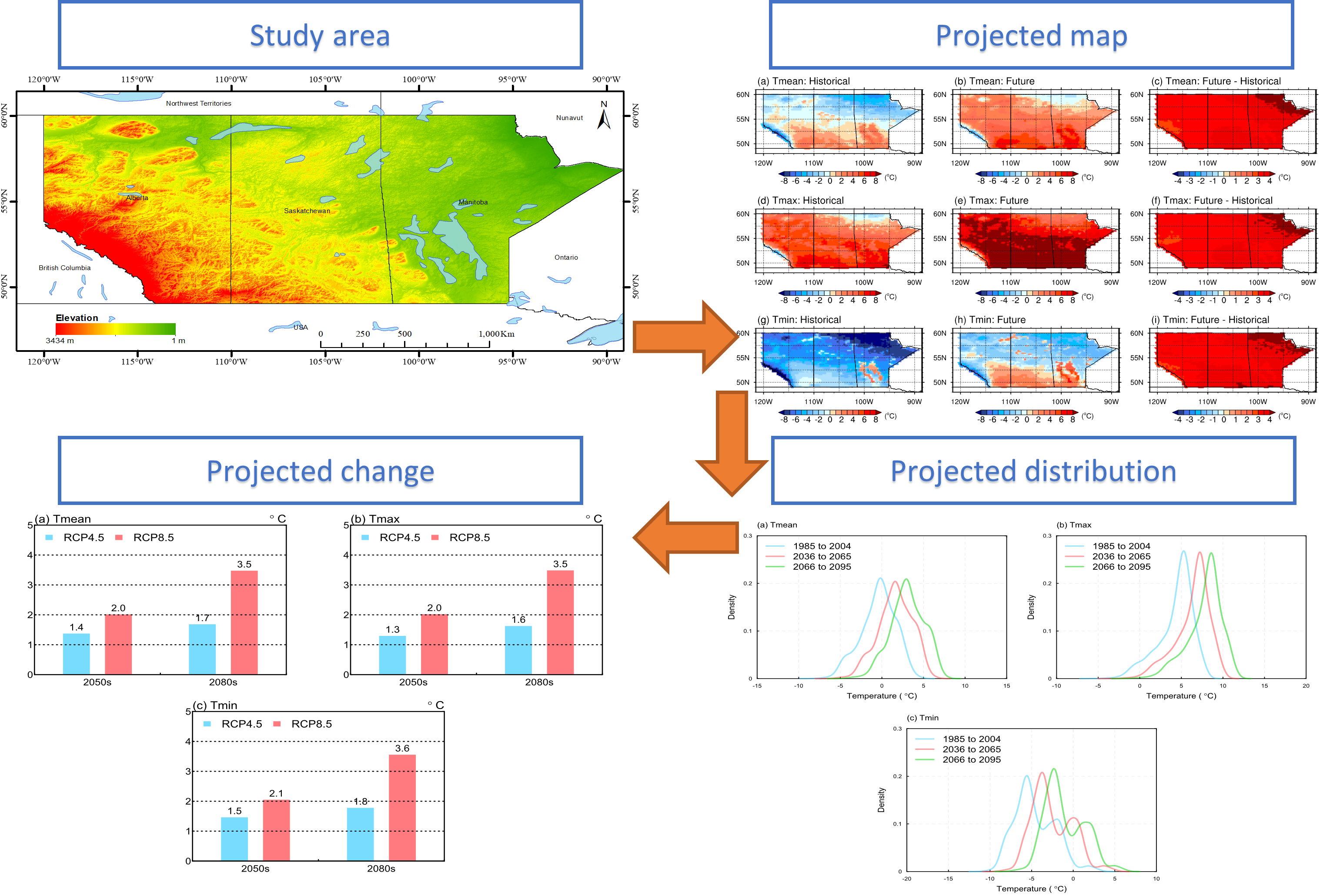
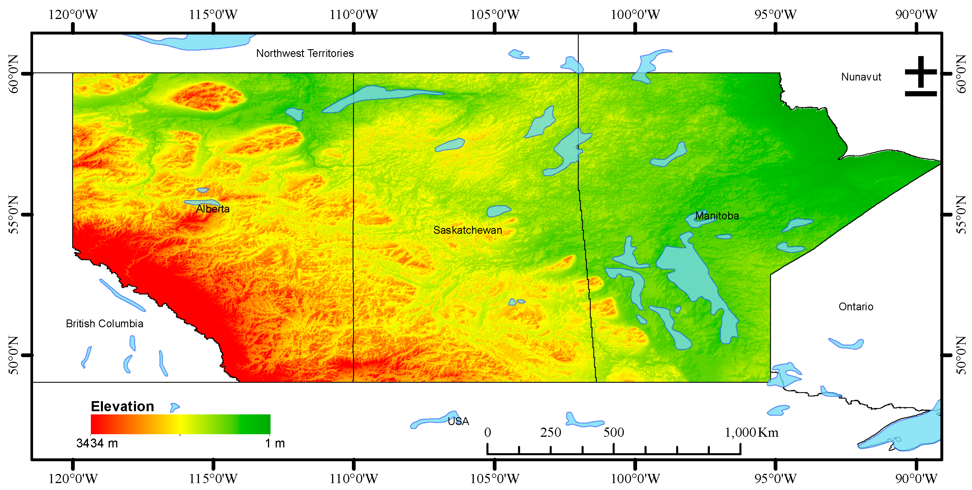
The study area is within the context of the Canadian Prairie Provinces, which include the Provinces of Manitoba, Saskatchewan, and Alberta. As shown in Figure 1, the topography in the study area is varied and complicated. The highest and lowest elevation is 3434 and 1 m, respectively. The Prairie Provinces have a total surface area of over 1,960,000 km2, accounting for 19.6% of the entire area of Canada [9]. Moreover, the climatic patterns of the Arctic and the Rocky Mountain have significant impacts on the climate of the Canadian Prairie Provinces [35,45].
A spatial experiment domain of 108 longitude × 128 latitude grid points with a horizontal resolution of 0.22° × 0.22° (i.e., approximately 25 km) is set up to cover the Prairie Provinces [9]. The land surface scheme is the 4.5 version of the Community Land Model (CLM4.5), while the multiple-phase cloud microphysics scheme is selected as the moisture scheme in RegCM4.6 [46]. The microphysics scheme is employed as the moisture scheme, while the lateral boundary condition scheme is the relaxation exponential technique [47,48]. The Holtslag PBL [49] is chosen as the boundary layer scheme and the cumulus convective scheme is the Emanuel scheme [50].
The annual average of daily maximum temperature over the Canadian Prairies in the period of 1960 to 2005 ranged from −4.0 to 12.6 °C, whereas daily minimum temperature varied from −12.2 to 0.6 °C. From 1960 to 2005, the maximum and minimum temperature increased by 1.5 and 2.3 °C, respectively. The spatial average of daily mean temperature for the period of 1960 to 2005 fluctuated from 3.7 to 7.3 °C, which increased by 1.6 °C since 1895 [9].
Intensified greenhouse-gas impacts and aggravated land-cover changes have contributed to increases in annual averages of daily maximum and minimum temperature [51]. It is expected that such increases would be amplified in the future, which can significantly affect the agriculture sector in the Canadian Prairies. Therefore, a higher spatial resolution of climate projections is needed to reveal the impacts of climate changes on the Canadian Prairies, and thus facilitate proper mitigative and adaptive strategies.
The historical climate observations over the Canadian Prairies were derived from a 10 km gridded climate dataset, which was produced by the National Land and Water Information Service (NLWIS), Agriculture and Agri-Food, Canada [52]. In this study, daily maximum and minimum temperatures in the period of 1985 to 2004 were extracted to analyze the annual averages within the study area. The elevation of the Canadian Prairie Provinces with a horizontal resolution of 30 arc-seconds was acquired from the Canadian Digital Elevation Data, which is developed by the Canadian Forestry Service, Ontario region [53].
The RegCM4.6 model is undertaken to dynamically downscale daily mean, maximum, and minimum temperature (expressed as Tmean, Tmax, and Tmin) over the Canadian Prairies. Annual averages of the daily temperatures for future periods of both 2036 to 2065 and 2066 to 2095 are calculated. The changes in temperature relative to the baseline period (i.e., 1985 to 2004) are then analyzed. Particularly, the changes in temperature (i.e., Vmean, Vmax, and Vmin) can be calculated as follows:
where , , and represent the annual average of daily mean, maximum, and minimum temperature in the future periods, respectively; whereas , , and indicate the annual average of daily mean, maximum, and minimum temperature for the historical period (i.e., 1985 to 2004). Detailed steps for projecting temperature variations through the RegCM4.6 model are summarized in Figure 2.
3. Projected Variations of Temperature
Previous studies have illustrated that RCMs are capable of capturing regional terrestrial and atmospheric processes as compared with GCMs [9,35]. The performance of RCMs in reproducing the historical temperature observations has been evaluated in previous studies [9,35,45,54,55,56,57,58,59,60]. Therefore, the development of fine-resolution temperature projections is the focus of this study. To comprehensively reveal how future temperature would be changed over the Canadian Prairies, temperature variations (i.e., Vmean, Vmax, and Vmin) in two future periods of both 2036 to 2065 and 2066 to 2095 under RCPs are analyzed with respective to the baseline period of 1985 to 2004.
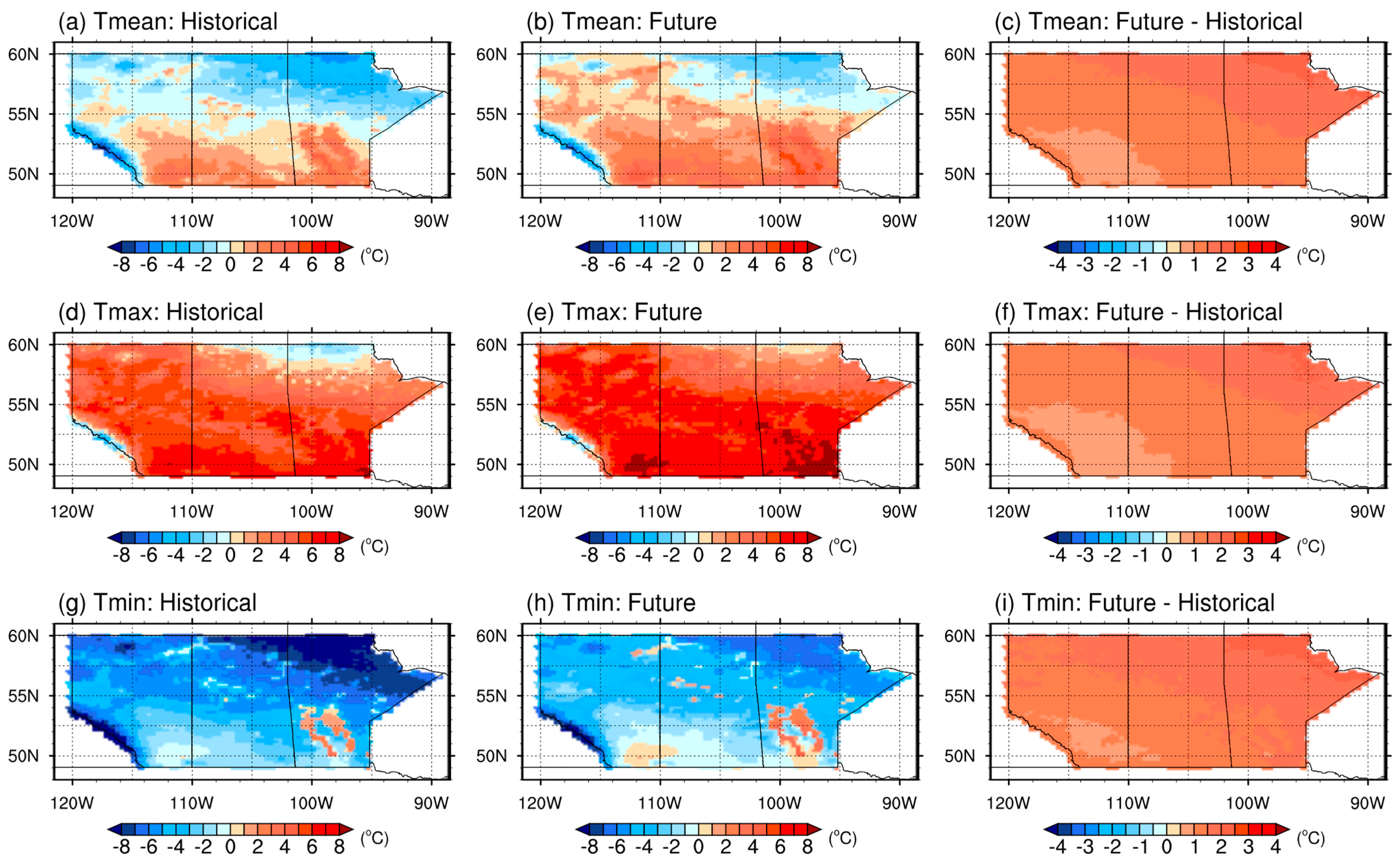
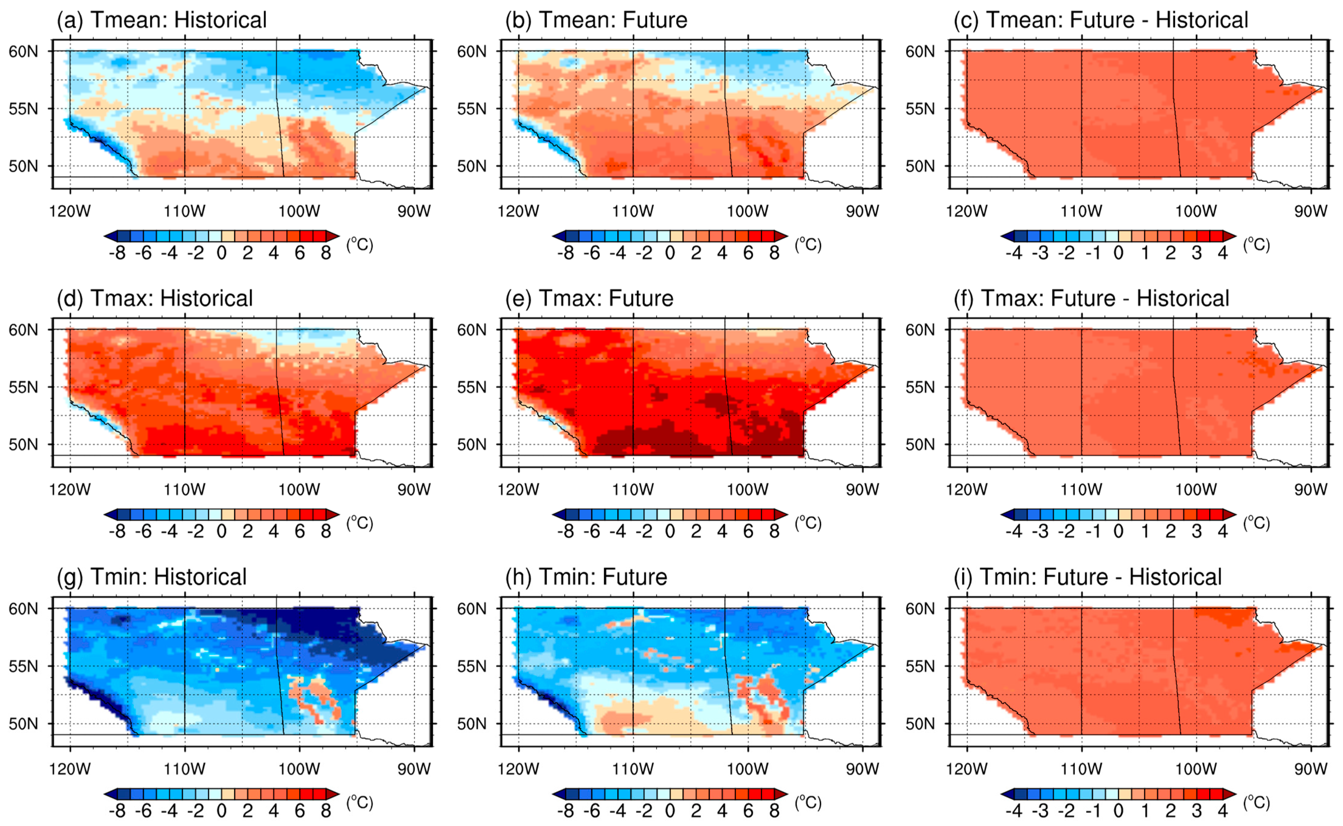
Figure 3 presents the projected variations of annual averages of Tmean, Tmax, and Tmin for the period of 2036 to 2065 under RCP45 relative to the baseline period. The figures in columns one and two show the spatial distribution of projected averages of daily temperatures for the historical and future period, respectively, whereas column three shows the calculated variations (i.e., Vmean, Vmax, and Vmin); rows one to three present Tmean, Tmax, and Tmin, respectively. For Tmean, the simulated spatial average and standard deviation over the entire area for the historical period are −0.4 and 2.1 °C, respectively (Figure 3a). It can be found that there is a decreasing pattern of the annual average from north to south. The spatial distribution from the future experiment in the period of 2036 to 2065 under RCP4.5 (Figure 3b) is closed to the historical one (Figure 3a), with an obviously increased magnitude. The result also indicates that the spatial average of Tmean over the provinces is projected to be 1.0 °C in the period of 2036 to 2065, where maximum and minimum values in the map reach −7.3 °C in the southwest and 5.8 °C in the southeast, respectively. However, a smaller standard deviation of 1.9 °C is projected for the period of 2036 to 2065, which indicates that the spatial variation would be reduced due to the increased magnitude of negative values under climate change. As shown in Figure 3c, the average of Tmean increases over the entire of the Prairie Provinces, with a northeastward-intensified pattern of projected changes. In addition, the RegCM model also simulates the largest increase at 56.60° N and 96.73° W in the northeast of Manitoba, and the smallest one at 51.47° N and 112.66° W in the southwest of Alberta.
Compared with Tmean, most of the spatial averages of Tmax are generally simulated to be above zero degrees, with the magnitude varying from −5.7 to 8.2 °C. The results derived from the RegCM model also show that Tmax has a spatial average of 4.3 °C and a standard deviation of 2.1 °C over the entire area for the historical period of 1985 to 2004 (Figure 3d). For the projected average of Tmax, generally the future (Figure 3e) and the historical (Figure 3d) experiments have a similar gradient pattern, but amplified values are revealed in the future period of 2036 to 2065. In particular, a spatial average of 5.6 °C over the Canadian Prairies is projected, with a standard deviation of 2.1 °C in the future period under RCP4.5. Figure 3f presents the projected variations of annual averages of Tmax for the future period relative to the baseline period. It can be observed that the entire Prairie Provinces would experience increases in Tmax, with a gradient intensified pattern from southwest to northeast. Likewise, the spatial average of Tmax would increase from 0.6 to 2.1 °C, while the most significant increase is found at the grid of 58.13° N and 94.91° W in the northeastern part.
In contrast, Tmin over the Prairie Provinces is almost below zero degrees, with a spatial average of −4.6 °C and a standard deviation of 2.4 °C (Figure 3g). It also indicated that greater spatial variations are presented in Tmin as compared with Tmax. The spatial pattern of both simulated historical and projected future average of Tmin matches each other quite well (Figure 3g,h), but with much greater values. A spatial average of −3.1 °C over the Canadian Prairies is projected, with a standard deviation of 2.2 °C in the period of 2036 to 2065 under RCP4.5. The greatest and smallest average are projected to be 3.4 °C in the southeast and −11.0 °C in the Rocky Mountain area, respectively. However, smaller spatial variations in the future might be caused by increased values of negative Tmin under climate change. The projected variations of annual averages of Tmin for the future period are presented in Figure 3i. Similar to Tmax during the future period, the annual averages of Tmin increase from 0.8 to 2.3 °C. It also can be observed that there is a gradient intensified pattern from southwest to northeast. Similarly, the most significant increase is located at 56.86° N and 88.97° W in the northeast, whereas the smallest one is at 51.47° N and 112.66° W in the southwest.
Moreover, Figure 4 depicts the annual averages of Tmean, Tmax, and Tmin for the period of 2066 to 2095 under RCP4.5, as well as their changes with respect to the baseline. Similarly, the spatial distributions of projected averages of daily temperatures for the historical and future period are shown in columns one and two, respectively. Column three depicts the computed changes in the projected values relative to the baseline period. In addition, the Tmean, Tmax, and Tmin respectively are presented in rows one to three. In general, there is a similar spatial distribution pattern of projected variations among Tmean, Tmax, and Tmin for the historical and future period. Similar to the revelations during the period of 2036 to 2065, the spatial average of Tmean, Tmax, and Tmin for the period of 2066 to 2095 increase by 1.7, 1.6, and 1.8 °C, respectively (Figure 4c,f,i). However, such increases are projected as slightly greater than those in the period 2036 to 2065 under RCP4.5. Moreover, the projected changes in the annual averages of Tmean, Tmax, and Tmin would be amplified from the southwest in the Rocky Mountain area to the northeast in the prairie region.
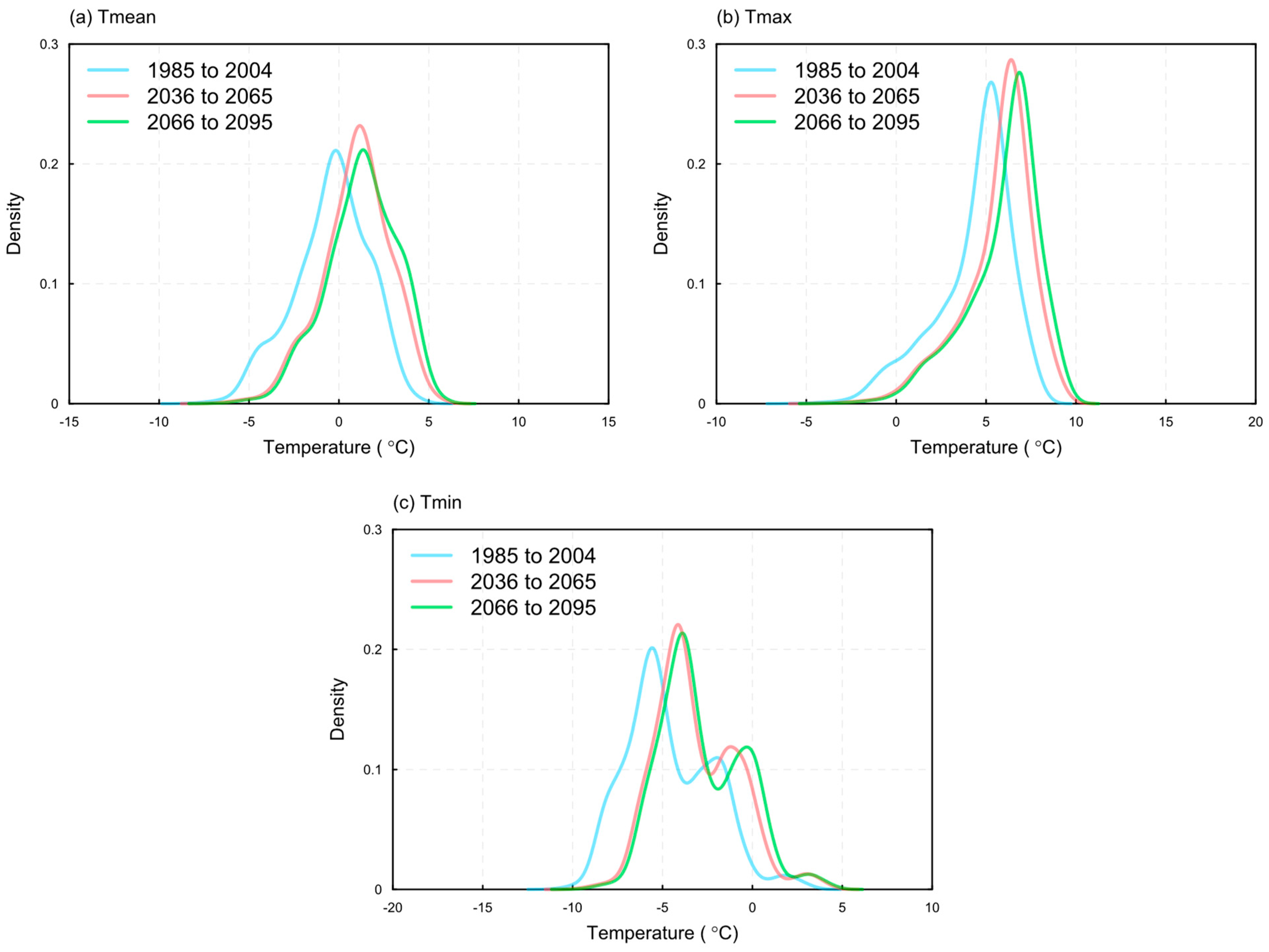
In order to further analyze the projected variations of Tmean, Tmax, and Tmin, the spatial distributions of their annual averages over the entire domain for the period of 2036 to 2065 and 2066 to 2095 under RCP4.5 are compared to those for the baseline period (Figure 5). In general, the shape of the distribution of Tmean, Tmax, and Tmin among three different periods matches each other. However, intensification of daily temperatures in the future is evident as shown from the changes of mean values, which is consistent with the previous revelations (Figure 3 and Figure 4). It can be observed that there is no significant difference in the projected changes between the period of 2036 to 2065 and the period of 2066 to 2095 in terms of the mean and standard deviation. For example, the mean and standard deviation of projections for Tmin in the period of 2036 to 2065 are projected to be −2.8 and 2.3 °C, respectively. Nevertheless, during the period of 2066 to 2095, the mean of projections is −3.1 °C with a standard deviation of 2.2 °C.
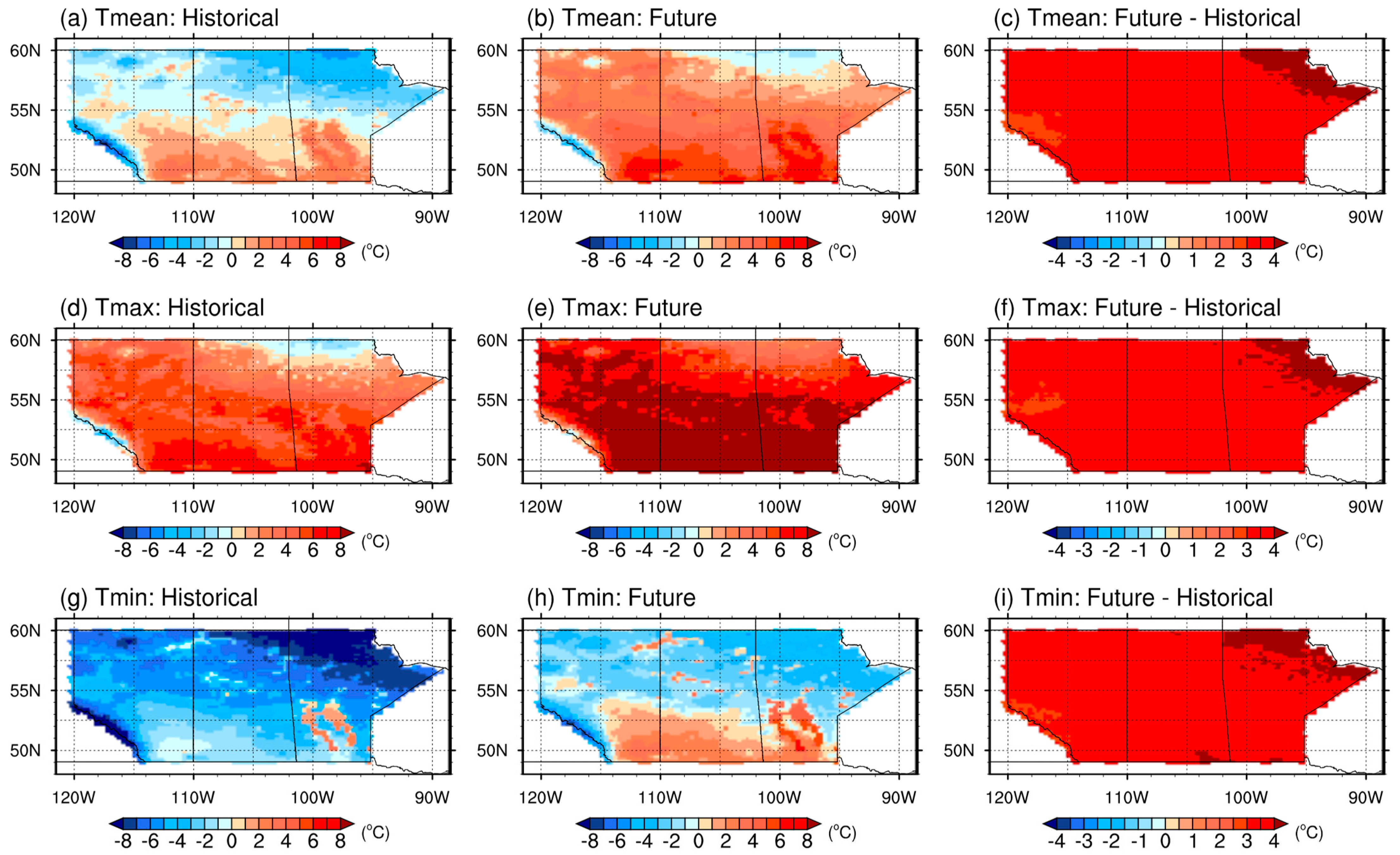
Figure 6 displays the projected annual averages of Tmean, Tmax, and Tmin for the period of 2036 to 2065 under RCP8.5. In the same way, the figures in columns one to three respectively present the simulated averages of daily temperatures for the historical and future periods, as well as their differences. The figures in rows one to three show Tmean, Tmax, and Tmin, respectively. Overall, the results show that the projections in the period of 2036 to 2065 under RCP8.5 are similar to those under RCP4.5. Moreover, there is an apparent warming pattern during the period of 2036 to 2065 under RCP8.5. For example, the RegCM model simulates the spatial averages of −4.6 and −2.5 °C for Tmin during the period 1985 to 2004 and 2036 to 2065, respectively. The largest average over the map during the future period of 2036 to 2065 is located at 50.20° N and 98.04° W in the southeast, nevertheless, the smallest one is at 52.19° N and 117.24° W in the southwest (Figure 6b). Moreover, significant increases under RCP8.5 are observed in the calculated differences between two periods. There is a similar intensified pattern from southwest to northeast, which is consistent with the results under RCP4.5.
To further analyze the temperature changes, Figure 7 presents the projected averages of Tmean, Tmax, and Tmin for the period of 2066 to 2095 under RCP8.5. Similar to the pattern during the period of 2036 to 2065 under RCP8.5, the increase in the averages would be reduced from the northeastern Prairie to the southeastern Rocky Mountain. However, it can be found that the projected increases during the period of 2066 to 2095 under RCP4.5 and RCP8.5 are significantly different from each other. For example, the maximum increases in annual averages of daily maximum temperature during the period of 2066 to 2095 under RCP4.5 and RCP8.5 are 2.5 and 4.5 °C, respectively. Such increases are amplified under RCP8.5 as caused by heavy GHG emissions.
The spatial distribution of annual averages over the entire Prairie Provinces for two future periods under RCP8.5 are in comparison with those for the baseline period (Figure 8). It is indicated that the distribution of Tmean, Tmax, and Tmin generally maintain the same shape among three different periods. Such revelations are also consistent with the results under RCP4.5. Nevertheless, the projected averages of daily temperatures are significantly intensified as seen from the shifted mean values. For example, the mean value of Tmax in the period of 2066 to 2095 is projected to be 6.0 °C under RCP4.5, whereas it is enlarged to 7.8 °C under RCP8.5.
4. Projected Trends of Temperature
In order to further explore the impacts of climate change on the Prairie Provinces, the Mann–Kendall (MK) test [61,62] and the non-parametric Theil–Sen (TS) estimator [63,64] were performed to reveal the temporal trends in annual averages of Tmean, Tmax, and Tmin at multiple stations under RCPs. In this study, sixteen spatially distributed stations are chosen, while more details can be referred to in Zhou et al. [9]. The probability of the MK test statistics and the magnitude of the TS estimator are examined for demonstrating how the Prairie Provinces are affected within the context of global warming.
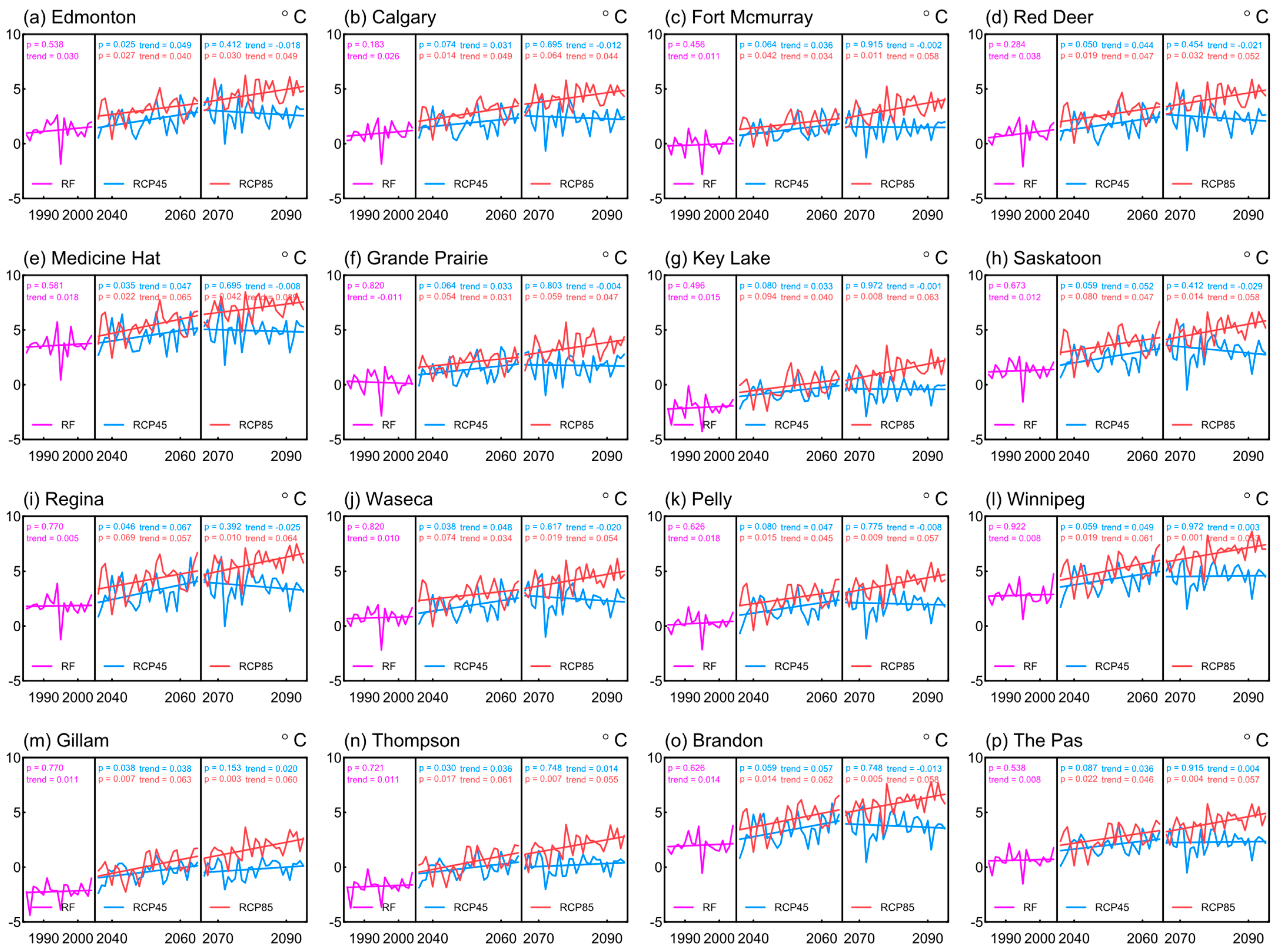
Figure 9 shows the time series and temporal trends of annual averages of Tmean at the 16 stations for two future periods under RCPs. It can be observed that the p-values of the MK test statistics at the majority of stations for future periods under RCP8.5 are less than the significance level (α = 0.05), indicating that there are significant trends in the annual averages of Tmean. Particularly, Tmean at all the stations in the period of 2066 to 2095 under RCP4.5 shows insignificant trends, ranging from −0.029 to 0.020 °C/year. This might be attributable to the stabilization of the population growth, land-use conversions, and greenhouse gas (GHG) emissions under RCP4.5 after the year 2050.
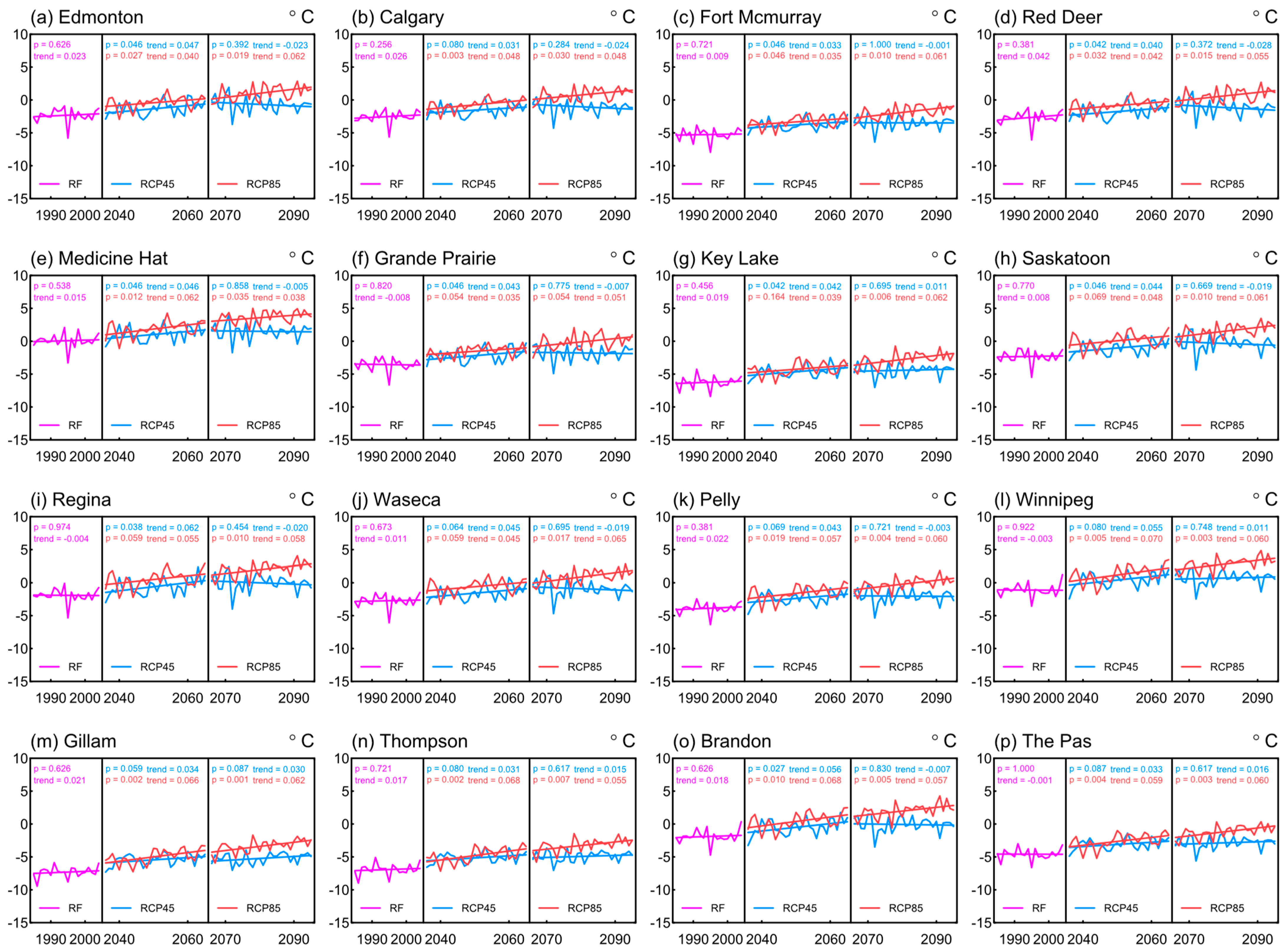
In addition, temporal trends are investigated for annual averages of Tmax and Tmin for future periods under RCPs, which are presented in Figure 10 and Figure 11, respectively. It can be noticed that similar warming trends are detected for the annual averages at all the stations under RCP8.5. However, the magnitude of positive trends in Tmean for most stations is generally smaller than Tmin, while larger than Tmax. This is also consistent with the results of projected variations, where larger increases are reported in Tmin. It is also evident that the trends in Tmax and Tmin at all the stations in the period of 2066 to 2095 under RCP4.5 are insignificant, as seen from the p-values of the MK test statistics.
5. Discussion
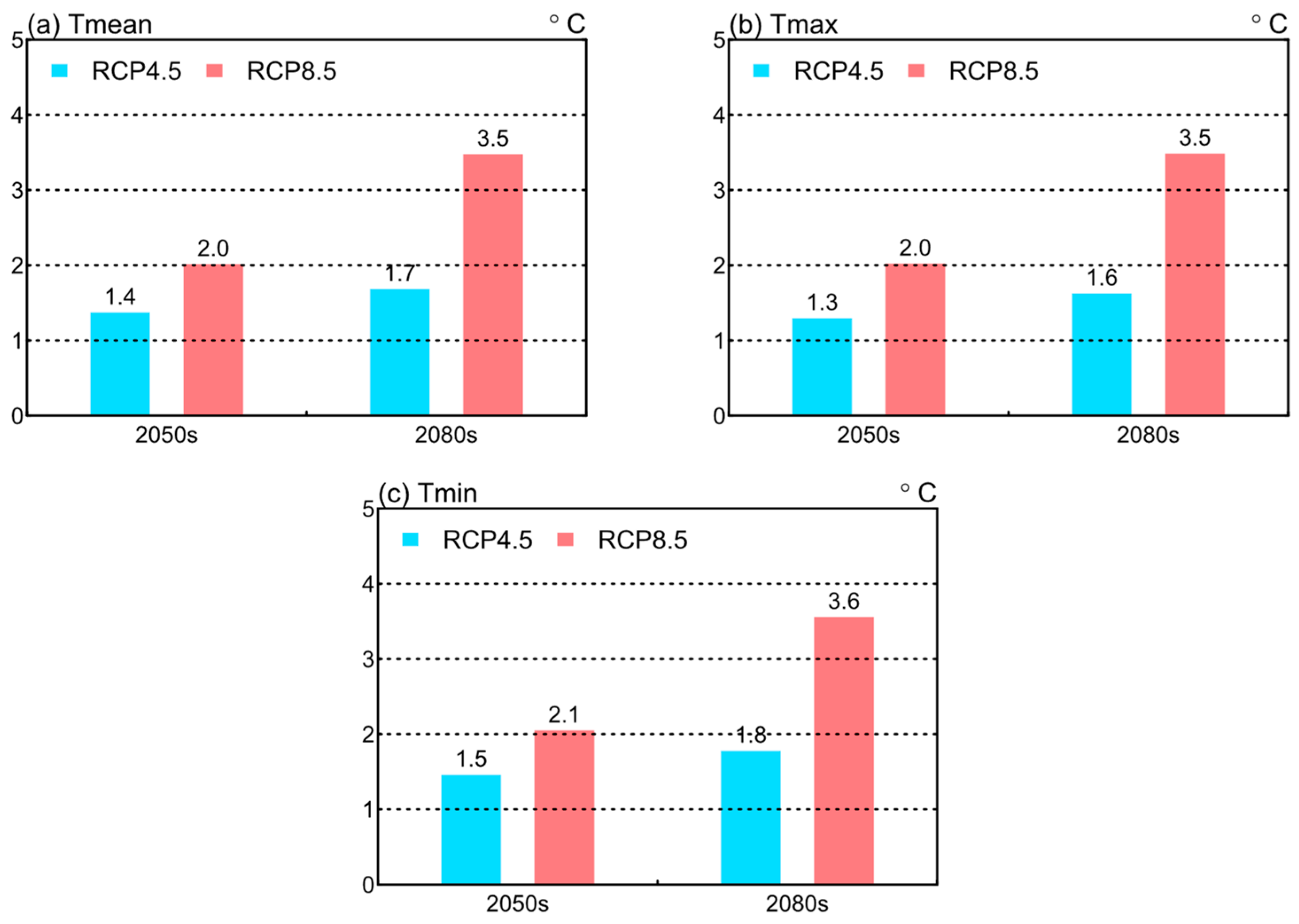
In this study, the Canadian Prairies shows a larger increase in the annual averages of Tmin than those of Tmax (Figure 12). This also implies that projected increases in annual averages of Tmax (Figure 12b) make a smaller contribution than Tmin (Figure 12c) to the increase in annual averages of Tmean (Figure 12a). The downscaling experiments also reveal that the trends in Tmean, Tmax, and Tmin at all the stations in the 2080s under RCP4.5 are insignificant. This might be attributable to the stabilization of population growth, land-use conversions, and greenhouse gas (GHG) emissions under RCP4.5 after the year 2050. Moreover, we found that greater increases in annual averages of daily temperatures are projected under RCP8.5 than those under RCP4.5, indicating that a higher emission scenario will initiate a more significant increase in temperatures due to greenhouse gas effects.
The projected results of temperature variations reveal that increases in the annual averages of daily temperatures would be intensified from the southwest in the Rocky Mountain area to the northeast in the prairie region. This is most likely due to the dynamic effects of a strong positive ice-snow albedo feedback, amplifying climate change as a result of decreasing ice-snow cover in the prairie region. The contribution of ice-snow albedo feedback to larger increases in the annual averages of Tmin in the northeast region would be more significant than Tmax due to a similar amplification effect. This is also consistent with the previous studies, which indicate that the high-latitude ice-snow albedo feedback is a primary element in projected increases in temperatures under the global warming scenarios [65,66,67].
6. Conclusions
In this study, dynamically downscaled variations of daily mean, maximum, and minimum temperature over the Canadian Prairies were developed through regional climate simulations. How the regional climate will increase in response to global warming in the future was thus analyzed. Specifically, RegCM was undertaken to downscale the boundary conditions of GFDL-ESM2M. Daily temperatures were subsequently extracted from the historical and future simulations. Temperature variations in the future periods (i.e., 2036 to 2065 and 2065 to 2095) are then investigated relative to the baseline period (i.e., 1985 to 2004). The spatial temperature distributions were analyzed to reveal the regional impacts of global warming on the Prairie Provinces.
The results suggested that the spatial distribution from the future experiment in the period of 2036 to 2065 under RCP4.5 is closed to the historical one, with an obviously increased magnitude. Moreover, it could be observed that there is no significant difference in the projected changes in temperatures between the period of 2036 to 2065 and the period of 2066 to 2095 in terms of their mean and standard deviation. The results further indicated that the projected changes would be amplified from the southwest in the Rocky Mountain area to the northeast in the prairie region. It was also suggested that the projected changes would be significantly intensified under RCP8.5. The projected variations of daily mean, minimum, and maximum temperature could provide scientific bases for adaptation and mitigation initiatives on multiple sectors, such as agriculture and economic sectors.
Significant increases in temperatures over the Canadian Prairies have been revealed through a comprehensive analysis of the projected variations. Such revealed increases can provide scientific bases for identifying appropriate adaptation and mitigation initiatives on multiple sectors. This study is limited since the RegCM model is merely driven by one GCM, which has difficulty in reflecting the uncertainties of boundary conditions. However, such boundary data provided by GCM outputs could significantly affect the projected temperature variations. Therefore, future research efforts can be extended to investigate the full potential ranges of temperature increases through dynamical downscaling of multiple GCMs.
Author Contributions
Conceptualization, X.Z.; methodology, X.Z.; software, X.Z.; validation, X.Z.; formal analysis, X.Z.; investigation, X.Z.; resources, X.Z., G.H. and Y.L.; data curation, X.Z., Q.L., D.Y. and X.H.; writing—original draft preparation, X.Z.; writing—review and editing, X.Z; visualization, X.Z.; supervision, G.H. and Y.L.; funding acquisition, Y.L. All authors have read and agreed to the published version of the manuscript.
Funding
This research is supported by the Natural Science Foundation of China (51779008, U2040212) and the Fundamental Research Funds for the Central Universities.
Acknowledgments
We are very grateful for the helpful inputs and suggestions from the editor and anonymous reviewers.
Conflicts of Interest
The authors declare no conflict of interest.
References
- Stern, P.C.; Perkins, J.H.; Sparks, R.E.; Knox, R.A. The challenge of climate-change neoskepticism. Science 2016, 353, 653–654. [Google Scholar] [CrossRef]
- McCreath, M. Report of the Conference on Climate Change and the Law of the Sea: Adapting the Law of the Sea to Address the Challenges of Climate Change, Centre for International Law, National University of Singapore, Singapore, 13–14 March 2018. Int. J. Mar. Coast. Law 2018, 33, 836–846. [Google Scholar] [CrossRef]
- Lewandowsky, S. Future Global Change and Cognition. Top. Cogn. Sci. 2016, 8, 7–18. [Google Scholar] [CrossRef] [PubMed] [Green Version]
- Lawson, E. Debrief: Meeting the climate change challenge. Br. J. Gen. Pract. 2019, 69, 343. [Google Scholar] [CrossRef]
- Kipling, R.; Topp, C.; Bannink, A.; Bartley, D.; Blanco-Penedo, I.; Cortignani, R.; del Prado, A.; Dono, G.; Faverdin, P.; Graux, A.-I.; et al. To what extent is climate change adaptation a novel challenge for agricultural modellers? Environ. Model. Softw. 2019, 120. [Google Scholar] [CrossRef]
- Balasubramanian, M. Climate change, famine, and low-income communities challenge Sustainable Development Goals. Lancet Planet. Health 2018, 2, e421–e422. [Google Scholar] [CrossRef] [Green Version]
- Argo, E.E. Migration Mismatch: Bird Migration and Phenological Mismatching. Am. Biol. Teach. 2018, 80, 540–543. [Google Scholar] [CrossRef]
- Abdulai, A. The challenges and adaptation to climate change by farmers in Sub-Saharan Africa. Agrekon 2018, 57, 28–39. [Google Scholar] [CrossRef]
- Zhou, X.; Huang, G.; Wang, X.; Fan, Y.; Cheng, G. A coupled dynamical-copula downscaling approach for temperature projections over the Canadian Prairies. Clim. Dyn. 2017, 51, 2413–2431. [Google Scholar] [CrossRef]
- Peel, M.C.; Srikanthan, R.; McMahon, T.A.; Karoly, D.J. Approximating uncertainty of annual runoff and reservoir yield using stochastic replicates of global climate model data. Hydrol. Earth Syst. Sci. 2015, 19, 1615–1639. [Google Scholar] [CrossRef] [Green Version]
- Nover, D.M.; Witt, J.W.; Butcher, J.; Johnson, T.E.; Weaver, C.P. The Effects of Downscaling Method on the Variability of Simulated Watershed Response to Climate Change in Five U.S. Basins. Earth Interact. 2016, 20, 1–27. [Google Scholar] [CrossRef] [PubMed]
- Lee, S.; Wallace, C.W.; Sadeghi, A.M.; Mccarty, G.W.; Zhong, H.; Yeo, I.-Y. Impacts of Global Circulation Model (GCM) bias and WXGEN on Modeling Hydrologic Variables. Water 2018, 10, 764. [Google Scholar] [CrossRef] [Green Version]
- Hosseinzadehtalaei, P.; Tabari, H.; Willems, P. Uncertainty assessment for climate change impact on intense precipitation: How many model runs do we need? Int. J. Clim. 2017, 37, 1105–1117. [Google Scholar] [CrossRef] [Green Version]
- Zhang, W.; Zhang, X.; Li, W.; Hou, N.; Wei, Y.; Jia, K.; Yao, Y.; Cheng, J. Evaluation of Bayesian Multimodel Estimation in Surface Incident Shortwave Radiation Simulation over High Latitude Areas. Remote Sens. 2019, 11, 1776. [Google Scholar] [CrossRef] [Green Version]
- Qiu, R.; Han, G.; Ma, X.; Xu, H.; Shi, T.; Zhang, M. A Comparison of OCO-2 SIF, MODIS GPP, and GOSIF Data from Gross Primary Production (GPP) Estimation and Seasonal Cycles in North America. Remote Sens. 2020, 12, 258. [Google Scholar] [CrossRef] [Green Version]
- Fu, Y.; Lu, X.; Zhao, Y.; Zeng, X.; Xia, L. Assessment Impacts of Weather and Land Use/Land Cover (LULC) Change on Urban Vegetation Net Primary Productivity (NPP): A Case Study in Guangzhou, China. Remote Sens. 2013, 5, 4125–4144. [Google Scholar] [CrossRef] [Green Version]
- Ahn, J.; Hong, S.; Cho, J.; Lee, Y.-W.; Lee, H. Statistical Modeling of Sea Ice Concentration Using Satellite Imagery and Climate Reanalysis Data in the Barents and Kara Seas, 1979–2012. Remote Sens. 2014, 6, 5520–5540. [Google Scholar] [CrossRef] [Green Version]
- Addo, K.A.; Larbi, L.; Amisigo, B.; Ofori-Danson, P.K. Impacts of Coastal Inundation Due to Climate Change in a CLUSTER of Urban Coastal Communities in Ghana, West Africa. Remote Sens. 2011, 3, 2029–2050. [Google Scholar] [CrossRef] [Green Version]
- Mika, A.M.; Weiss, R.M.; Olfert, O.; Hallett, R.H.; Newman, J. Will climate change be beneficial or detrimental to the invasive swede midge in North America? Contrasting predictions using climate projections from different general circulation models. Glob. Chang. Biol. 2008, 14, 1721–1733. [Google Scholar] [CrossRef]
- McGinn, S.M.; Shepherd, A. Impact of climate change scenarios on the agroclimate of the Canadian prairies. Can. J. Soil Sci. 2003, 83, 623–630. [Google Scholar] [CrossRef]
- Thorpe, J.; Wolfe, S.A.; Houston, B. Potential impacts of climate change on grazing capacity of native grasslands in the Canadian prairies. Can. J. Soil Sci. 2008, 88, 595–609. [Google Scholar] [CrossRef]
- Bonsal, B.; Liu, Z.; Wheaton, E.; Stewart, R. Historical and Projected Changes to the Stages and Other Characteristics of Severe Canadian Prairie Droughts. Water 2020, 12, 3370. [Google Scholar] [CrossRef]
- Wotton, B.M.; Martell, D.L.; Logan, K.A. Climate Change and People-Caused Forest Fire Occurrence in Ontario. Clim. Chang. 2003, 60, 275–295. [Google Scholar] [CrossRef]
- Thorne, R. Uncertainty in the impacts of projected climate change on the hydrology of a subarctic environment: Liard River Basin. Hydrol. Earth Syst. Sci. 2011, 15, 1483–1492. [Google Scholar] [CrossRef] [Green Version]
- Sultana, Z.; Coulibaly, P. Distributed modelling of future changes in hydrological processes of Spencer Creek watershed. Hydrol. Process. 2010, 25, 1254–1270. [Google Scholar] [CrossRef]
- Shrestha, R.R.; Schnorbus, M.A.; Werner, A.T.; Zwiers, F.W. Evaluating Hydroclimatic Change Signals from Statistically and Dynamically Downscaled GCMs and Hydrologic Models. J. Hydrometeorol. 2014, 15, 844–860. [Google Scholar] [CrossRef]
- Schertzer, W.M.; Croley, T.E. Climate change impact on hydrology and lake thermal structure. In Proceedings of the 27th Congress of the International-Association-for-Hydraulic-Research, San Francisco, CA, USA, 10–15 August 1997; pp. 919–924. [Google Scholar]
- Mahat, V.; Anderson, A. Impacts of climate and catastrophic forest changes on streamflow and water balance in a mountainous headwater stream in Southern Alberta. Hydrol. Earth Syst. Sci. 2013, 17, 4941–4956. [Google Scholar] [CrossRef] [Green Version]
- Cheng, C.S.; Lopes, E.; Fu, C.; Huang, Z. Possible Impacts of Climate Change on Wind Gusts under Downscaled Future Climate Conditions: Updated for Canada. J. Clim. 2014, 27, 1255–1270. [Google Scholar] [CrossRef]
- Bonsal, B.R.; Prowse, T.D.; Pietroniro, A. An assessment of global climate model-simulated climate for the western cordillera of Canada (1961–90). Hydrol. Process. 2003, 17, 3703–3716. [Google Scholar] [CrossRef]
- St-Jacques, J.-M.; Andreichuk, Y.; Sauchyn, D.J.; Barrow, E. Projecting Canadian Prairie Runoff for 2041-2070 with North American Regional Climate Change Assessment Program (NARCCAP) Data. JAWRA J. Am. Water Resour. Assoc. 2018, 54, 660–675. [Google Scholar] [CrossRef]
- Qian, B.; Wang, H.; He, Y.; Liu, J.; De Jong, R. Projecting spring wheat yield changes on the Canadian Prairies: Effects of resolutions of a regional climate model and statistical processing. Int. J. Clim. 2015, 36, 3492–3506. [Google Scholar] [CrossRef] [Green Version]
- PaiMazumder, D.; Sushama, L.; Laprise, R.; Khaliq, M.N.; Sauchyn, D. Canadian RCM projected changes to short- and long-term drought characteristics over the Canadian Prairies. Int. J. Clim. 2012, 33, 1409–1423. [Google Scholar] [CrossRef]
- Kerr, S.A.; Andreichuk, Y.; Sauchyn, D.J. Re-Evaluating the Climate Factor in Agricultural Land Assessment in a Changing Climate—Saskatchewan, Canada. Land 2019, 8, 49. [Google Scholar] [CrossRef] [Green Version]
- Zhou, X.; Huang, G.; Piwowar, J.; Fan, Y.; Wang, X.; Li, Z.; Cheng, G. Hydrologic Impacts of Ensemble-RCM-Projected Climate Changes in the Athabasca River Basin, Canada. J. Hydrometeorol. 2018, 19, 1953–1971. [Google Scholar] [CrossRef] [Green Version]
- Schumacher, V.; Fernández, A.; Justino, F.; Comin, A. WRF High Resolution Dynamical Downscaling of Precipitation for the Central Andes of Chile and Argentina. Front. Earth Sci. 2020, 8, 328. [Google Scholar] [CrossRef]
- Shalaby, A.; Zakey, A.S.; Tawfik, A.B.; Solmon, F.; Giorgi, F.; Stordal, F.; Sillman, S.; Zaveri, R.A.; Steiner, A.L. Implementation and evaluation of online gas-phase chemistry within a regional climate model (RegCM-CHEM4). Geosci. Model Dev. 2012, 5, 741–760. [Google Scholar] [CrossRef] [Green Version]
- Sylla, M.; Giorgi, F.; Stordal, F. Large-Scale origins of rainfall and temperature bias in high-resolution simulations over southern Africa. Clim. Res. 2012, 52, 193–211. [Google Scholar] [CrossRef] [Green Version]
- Zampieri, M.; Lionello, P. Anthropic land use causes summer cooling in Central Europe. Clim. Res. 2011, 46, 255–268. [Google Scholar] [CrossRef] [Green Version]
- Maurya, R.K.S.; Mohanty, M.R.; Sinha, P.; Mohanty, U.C. Performance of hydrostatic and non-hydrostatic dynamical cores in RegCM4.6 for Indian summer monsoon simulation. Meteorol. Appl. 2020, 27, e1915. [Google Scholar] [CrossRef]
- Balov, M.N.; Altunkaynak, A. Trend Analyses of Extreme Precipitation Indices Based on Downscaled Outputs of Global Circulation Models in Western Black Sea Basin, Turkey. Iran. J. Sci. Technol. Trans. Civ. Eng. 2019, 43, 821–834. [Google Scholar] [CrossRef]
- Kohyama, T.; Hartmann, D.L.; Battisti, D.S. La Niña–like Mean-State Response to Global Warming and Potential Oceanic Roles. J. Clim. 2017, 30, 4207–4225. [Google Scholar] [CrossRef]
- Matveeva, T.A.; Gushchina, D.Y.; Zolina, O.G. Large-Scale indicators of extreme precipitation in coastal natural-economic zones of the European part of Russia. Russ. Meteorol. Hydrol. 2015, 40, 722–730. [Google Scholar] [CrossRef]
- Ng, B.; Cai, W.; Walsh, K. Nonlinear Feedbacks Associated with the Indian Ocean Dipole and Their Response to Global Warming in the GFDL-ESM2M Coupled Climate Model. J. Clim. 2014, 27, 3904–3919. [Google Scholar] [CrossRef]
- Zhou, X.; Huang, G.; Wang, X.; Cheng, G. Dynamically-Downscaled temperature and precipitation changes over Saskatchewan using the PRECIS model. Clim. Dyn. 2017, 50, 1321–1334. [Google Scholar] [CrossRef]
- Fisher, R.A.; Muszala, S.; Verteinstein, M.; Lawrence, P.; Xu, C.; McDowell, N.G.; Knox, R.G.; Koven, C.; Holm, J.; Rogers, B.M.; et al. Taking off the training wheels: The properties of a dynamic vegetation model without climate envelopes, CLM4.5(ED). Geosci. Model Dev. 2015, 8, 3593–3619. [Google Scholar] [CrossRef] [Green Version]
- Adeniyi, M.O. Sensitivity of different convection schemes in RegCM4. 0 for simulation of precipitation during the Septembers of 1989 and 1998 over West Africa. Theor. Appl. Climatol. 2014, 115, 305–322. [Google Scholar] [CrossRef]
- Davies, H.C. A lateral boundary formulation for multi-level prediction models. Q. J. R. Meteorol. Soc. 1976, 102, 405–418. [Google Scholar] [CrossRef]
- Holtslag, A.; De Bruijn, E.; Pan, H.L. A high resolution air mass transformation model for short-range weather forecasting. Mon. Weather Rev. 1990, 118, 1561–1575. [Google Scholar] [CrossRef]
- Emanuel, K.A.; Živković-Rothman, M. Development and evaluation of a convection scheme for use in climate models. J. Atmos. Sci. 1999, 56, 1766–1782. [Google Scholar] [CrossRef] [Green Version]
- Skinner, W.; Majorowicz, J. Regional climatic warming and associated twentieth century land-cover changes in north-western North America. Clim. Res. 1999, 12, 39–52. [Google Scholar] [CrossRef] [Green Version]
- NLWIS. A Daily 10 km Gridded Climate Dataset for Canada, 1961–2003. Available online: https://www.mcgill.ca/library/find/maps/dgcd10km (accessed on 14 February 2017).
- Natural Resources Canada. Canada 3D—Digital Elevation Model of the Canadian Landmass. Available online: https://open.canada.ca/data/en/dataset/042f4628-94b2-40ac-9bc1-ca3ac2a27d82 (accessed on 14 July 2021).
- Jeong, D.I.; Sushama, L.; Diro, G.T.; Khaliq, M.N. Projected changes to winter temperature characteristics over Canada based on an RCM ensemble. Clim. Dyn. 2015, 47, 1351–1366. [Google Scholar] [CrossRef] [Green Version]
- Mladjic, B.; Sushama, L.; Khaliq, M.N.; Laprise, R.; Caya, D.; Roy, R. Canadian RCM Projected Changes to Extreme Precipitation Characteristics over Canada. J. Clim. 2011, 24, 2565–2584. [Google Scholar] [CrossRef] [Green Version]
- Plummer, D.A.; Caya, D.; Frigon, A.; Côté, H.; Giguère, M.; Paquin, D.; Biner, S.; Harvey, R.; De Elia, R. Climate and Climate Change over North America as Simulated by the Canadian RCM. J. Clim. 2006, 19, 3112–3132. [Google Scholar] [CrossRef]
- Sushama, L.; Khaliq, N.; Laprise, R. Dry spell characteristics over Canada in a changing climate as simulated by the Canadian RCM. Glob. Planet. Chang. 2010, 74, 1–14. [Google Scholar] [CrossRef]
- Jeong, D.I.; Sushama, L.; Diro, G.T.; Khaliq, M.N.; Beltrami, H.; Caya, D. Projected changes to high temperature events for Canada based on a regional climate model ensemble. Clim. Dyn. 2015, 46, 3163–3180. [Google Scholar] [CrossRef]
- Zhou, X.; Huang, G.; Baetz, B.W.; Wang, X.; Cheng, G. PRECIS-Projected increases in temperature and precipitation over Canada. Q. J. R. Meteorol. Soc. 2018, 144, 588–603. [Google Scholar] [CrossRef]
- Zhou, X.; Huang, G.; Wang, X.; Cheng, G. Future Changes in Precipitation Extremes over Canada: Driving Factors and Inherent Mechanism. J. Geophys. Res. Atmos. 2018, 123, 5783–5803. [Google Scholar] [CrossRef]
- Mann, H.B. Nonparametric tests against trend. Econom. J. Econom. Soc. 1945, 13, 245–259. [Google Scholar] [CrossRef]
- Kendall, M.G. Rank Correlation Methods; Griffin: Oxford, UK, 1948. [Google Scholar]
- Theil, H. A rank-invariant method of linear and polynomial regression analysis. In Henri Theil’s Contributions to Economics and Econometrics; Springer: Berlin/Heidelberg, Germany, 1992; pp. 345–381. [Google Scholar]
- Sen, P.K. Estimates of the regression coefficient based on Kendall’s tau. J. Am. Stat. Assoc. 1968, 63, 1379–1389. [Google Scholar] [CrossRef]
- Gorodetskaya, I.; Cane, M.A.; Tremblay, L.; Kaplan, A. The effects of sea-ice and land-snow concentrations on planetary albedo from the earth radiation budget experiment. Atmos. Ocean 2006, 44, 195–205. [Google Scholar] [CrossRef]
- Pierrehumbert, R.T. Climate dynamics of a hard snowball Earth. J. Geophys. Res. Space Phys. 2005, 110, D01111. [Google Scholar] [CrossRef]
- Sorteberg, A.; Kattsov, V.; Walsh, J.; Pavlova, T. The Arctic surface energy budget as simulated with the IPCC AR4 AOGCMs. Clim. Dyn. 2007, 29, 131–156. [Google Scholar] [CrossRef]
Figure 1.
Topography of the study area.

Figure 2.
Methodological framework for projecting temperature variations.

Figure 3.
Projected variations of annual averages of Tmean, Tmax, and Tmin for the period of 2036 to 2065 under RCP45. (a,d,g) show the historical distributions of Tmean, Tmax, and Tmin, respectively; (b,e,h) show the future distributions of Tmean, Tmax, and Tmin, respectively; (c,f,i) show the projected variations of Vmean, Vmax, and Vmin, respectively.

Figure 4.
Projected variations of annual averages of Tmean, Tmax, and Tmin for the period of 2066 to 2095 under RCP45. (a,d,g) show the historical distributions of Tmean, Tmax, and Tmin, respectively; (b,e,h) show the future distributions of Tmean, Tmax, and Tmin, respectively; (c,f,i) show the projected variations of Vmean, Vmax, and Vmin, respectively.

Figure 5.
Spatial distribution of annual averages for the historical and future periods under RCP45. (a) Tmean, (b) Tmax, and (c) Tmin.
Figure 5.
Spatial distribution of annual averages for the historical and future periods under RCP45. (a) Tmean, (b) Tmax, and (c) Tmin.

Figure 6.
Projected variations of annual averages of Tmean, Tmax, and Tmin for the period of 2036 to 2065 under RCP85. (a,d,g) show the historical distributions of Tmean, Tmax, and Tmin, respectively; (b,e,h) show the future distributions of Tmean, Tmax, and Tmin, respectively; (c,f,i) show the projected variations of Vmean, Vmax, and Vmin, respectively.

Figure 7.
Projected variations of annual averages of Tmean, Tmax, and Tmin for the period of 2066 to 2095 under RCP85. (a,d,g) show the historical distributions of Tmean, Tmax, and Tmin, respectively; (b,e,h) show the future distributions of Tmean, Tmax, and Tmin, respectively; (c,f,i) show the projected variations of Vmean, Vmax, and Vmin, respectively.

Figure 8.
Spatial distribution of annual averages for the historical and future periods under RCP85. (a) Tmean, (b) Tmax, and (c) Tmin.
Figure 8.
Spatial distribution of annual averages for the historical and future periods under RCP85. (a) Tmean, (b) Tmax, and (c) Tmin.

Figure 9.
Temporal trends in annual averages of Tmean at the 16 stations. The value of p and trend is derived from the MK test and the Theil–Sen estimator, respectively. The straight line represents the linear trend derived from the Theil–Sen estimator. (a) Edmonton, (b) Calgary, (c) Fort Mcmurray, (d) Red Deer, (e) Medicine Hat, (f) Grande Prairie, (g) Key Lake, (h) Saskatoon, (i) Regina, (j) Waseca, (k) Pelly, (l) Winnipeg, (m) Gillam, (n) Thompson, (o) Brandon, and (p) The Pas.

Figure 10.
Temporal trends in annual averages of Tmax at the 16 stations. The value of p and trend is derived from the MK test and the Theil–Sen estimator, respectively. The straight line represents the linear trend derived from the Theil–Sen estimator. (a) Edmonton, (b) Calgary, (c) Fort Mcmurray, (d) Red Deer, (e) Medicine Hat, (f) Grande Prairie, (g) Key Lake, (h) Saskatoon, (i) Regina, (j) Waseca, (k) Pelly, (l) Winnipeg, (m) Gillam, (n) Thompson, (o) Brandon, and (p) The Pas.

Figure 11.
Temporal trends in annual averages of Tmin at the 16 stations. The value of p and trend is derived from the MK test and the Theil–Sen estimator, respectively. The straight line represents the linear trend derived from the Theil–Sen estimator. (a) Edmonton, (b) Calgary, (c) Fort Mcmurray, (d) Red Deer, (e) Medicine Hat, (f) Grande Prairie, (g) Key Lake, (h) Saskatoon, (i) Regina, (j) Waseca, (k) Pelly, (l) Winnipeg, (m) Gillam, (n) Thompson, (o) Brandon, and (p) The Pas.

Figure 12.
Spatial averages of projected changes for the future periods under RCPs. (a) Tmean, (b) Tmax, and (c) Tmin.
Figure 12.
Spatial averages of projected changes for the future periods under RCPs. (a) Tmean, (b) Tmax, and (c) Tmin.

Publisher’s Note: MDPI stays neutral with regard to jurisdictional claims in published maps and institutional affiliations. |
© 2021 by the authors. Licensee MDPI, Basel, Switzerland. This article is an open access article distributed under the terms and conditions of the Creative Commons Attribution (CC BY) license (https://creativecommons.org/licenses/by/4.0/).
Share and Cite
MDPI and ACS Style
Zhou, X.; Huang, G.; Li, Y.; Lin, Q.; Yan, D.; He, X. Dynamical Downscaling of Temperature Variations over the Canadian Prairie Provinces under Climate Change. Remote Sens. 2021, 13, 4350. https://doi.org/10.3390/rs13214350
AMA Style
Zhou X, Huang G, Li Y, Lin Q, Yan D, He X. Dynamical Downscaling of Temperature Variations over the Canadian Prairie Provinces under Climate Change. Remote Sensing. 2021; 13(21):4350. https://doi.org/10.3390/rs13214350
Chicago/Turabian StyleZhou, Xiong, Guohe Huang, Yongping Li, Qianguo Lin, Denghua Yan, and Xiaojia He. 2021. "Dynamical Downscaling of Temperature Variations over the Canadian Prairie Provinces under Climate Change" Remote Sensing 13, no. 21: 4350. https://doi.org/10.3390/rs13214350
Note that from the first issue of 2016, this journal uses article numbers instead of page numbers. See further details here.