
Estimating Snowpack Density from Near-Infrared Spectral Reflectance Using a Hybrid Model


Institut National de la Recherche Scientifique (INRS), Québec, QC G1K 9A9, Canada
*
Author to whom correspondence should be addressed.
Remote Sens. 2021, 13(20), 4089; https://doi.org/10.3390/rs13204089
Submission received: 6 August 2021
/
Revised: 4 October 2021
/
Accepted: 7 October 2021
/
Published: 13 October 2021
Abstract
:Improving the estimation of snow density is a key task in current snow research. Characterization of the variability of density in time and space is essential for the estimation of water equivalent, hydroelectric power production, assessment of natural hazards (avalanches, floods, etc.). Hyperspectral imaging is proving to be a promising and reliable tool for monitoring and estimating this physical property. Indeed, the spectral reflectance of snow is partly controlled by changes in its physical properties, particularly in the near-infrared (NIR) part of the spectrum. For this purpose, several models have been designed to estimate snow density from spectral information. However, none has yet achieved significant performance. One of the major difficulties is that the relationship between snow density and spectral reflectance is non-bijective (surjective). Indeed, several reflectance amplitudes can be associated with the same density and vice versa, so the correlation between density and spectral reflectance can be very poor. To resolve this issue, a hybrid snow density estimation model based on spectral data is proposed in this work. The principle behind this model is to classify the snow density prior to its estimation by means of a specific estimator corresponding to a predetermined snow density class. These additional steps eliminate the surjective relation by converting it into three bijective relations between density and spectral reflectance. The calibration step showed that the densities included within the three classes are sensitive to different spectral regions, with R2 > 0.80. The results of the cross-validation for the specific estimators were also satisfactory with R2 > 0.78 and RMSE < 36.36 kg m−3. The overall performance of the hybrid model (HM), when tested with independent data, demonstrated the effectiveness of using proximal NIR hyperspectral imagery to estimate snow density (R2 = NASH = 0.93).
1. Introduction
The spatiotemporal evolution of seasonal snowpacks is an important indicator of climate [1]. The measurement, monitoring, and management of this water resource are of great interest to governments and the scientific community. Snow cover is the set of snow layers that accumulate on the ground throughout the winter [2]. Each of these layers has a given density. Quantifying the variability of density in time and space is essential for estimating the water equivalent [3,4], hydroelectric power production [5,6], and assessing natural hazards (avalanches, floods, etc.) [7,8]. Indeed, this variable varies with changes in other physical properties such as grain size, grain shape, and liquid water content during the metamorphic transformation of the snowpack [9]. The density of newly deposited snow is expected to have the lowest values and to increase and reach its highest values during the maturation phase. According to Pomeroy et al. [10], the typical seasonal density of the snowpack ranges between 80 kg m−3 and 600 kg m−3.
For a country like Canada, which covers a very large area with a vast expanse of snow cover, regular monitoring of snow density is important [11,12]. The density is measured using a variety of methods and technologies. These include manual measurements by taking core samples from the snowpack (such as ‘federal’ snow tubes, e.g., ESC-30) [13], or the installation of devices that lie flat on the ground and weigh the snow as it accumulates on top (such as snow pillows) [14,15]. However, each of these methods has several drawbacks [15,16]. Snow core measurements are labor intensive, time-consuming, not feasible for 24-h data collection, and subject to human error. Snow pillows have measurement errors, logistical and transport problems for their installation, and can only measure an area of about 10 m2 [15]. There are also other methods for measuring snow density, including proximal remote sensing (such as the GMON (GammaMONitor) snow water equivalent probe (Campbell Scientific Canada, Edmonton, AB, Canada)) [17], spatial remote sensing (microwave remote sensing) [18]. However, these methods have some drawbacks; for example, they do not measure the density of each snow layer that makes up the vertical stratigraphy of the snowpack, but only the average density of the snowpack. Recently, optical sensor data have been used as an alternative to monitor snow cover over large areas and have led to improved monitoring and management of this water resource [19]. To optimize the modeling process of the physical properties of snow and to develop new efficient models, a high spectral resolution is essential [20].
Hyperspectral imaging technology is an innovative approach based on spectroscopic analyses. It is fast, non-invasive, and facilitates real-time measurements [21,22], which can be used in conjunction with traditional measurement methods. This technology has proven to be effective for field, laboratory, and industrial applications [23,24]. It provides detailed information about the physical and chemical components of a scanned sample due to its high spectral and temporal resolution [23,25,26]. It has already been demonstrated that the near-infrared (NIR) spectrum is sensitive to the physical parameters of snow [27,28,29,30]. In fact, snow granulometry is clearly visible in the NIR and the short waves of infrared regions (SWIR) [31,32]. Eppanapelli et al. [33] found that the spectral reflectance of snow in the NIR is inversely proportional to the liquid water content in the snow. In addition, the absorption of ice in the NIR is very high [34], so the effect of impurities such as mineral dust and soot is negligible beyond 1000 nm wavelength. The above findings highlight the potential of hyperspectral NIR data to gather information on the physical properties of snow for modeling purposes [35].
Indeed, several models and approaches designed to model snow density based on spectral data are now available, but none has yet achieved a satisfactory performance [36,37]. This is probably due to the fact that most models are based on the assumption that density measurements can be modeled using the same function. Even though the spectral reflectance of snow in the NIR depends on density, it is expressed by the size and shape of the grains (granulometry) and the liquid water content in the snow [38]. Consequently, the optical properties of the physical parameters of snow influence one another and create a non-bijective (surjective (In mathematics, a surjective function (also known as surjection, or onto function) is a function f that maps an element x to every element y; that is, for every y, there is an x such that f(x) = y.)) relationship between snow density and reflectance in the NIR, resulting in poor correlations.
Recently, it has been demonstrated that three optical classes of snow with different degrees of metamorphosis (weakly to moderately metamorphosed (WMM), moderately to highly metamorphosed (MHM), and highly to very highly metamorphosed (HVM)) can be identified and discriminated against without prior recognition, based only on NIR hyperspectral data [39]. This study showed that the spectra of snow density are similar within the same optical class and significantly different from one optical class to another. In other words, densities expressed in terms of grain size, shape, and spectral response were discriminated and grouped into three different homogeneous subclasses [39]. With this finding, it is possible to train estimators specific to the identified homogeneous classes, which are governed by a bijective (In mathematics, a bijection, bijective function, one-to-one correspondence, or invertible function, is a function between the elements of two sets, where each element of one set is paired with exactly one element of the other set, and each element of the other set is paired with exactly one element of the first set. There are no unpaired elements.) relation between the density and the hyperspectral NIR reflectance.
The objective of this study is to develop a hybrid model (HM) to estimate the snow density using proximal NIR hyperspectral data. The HM is a combination of a classifier and specific estimators associated with three density classes (WMM, MHM, and HVM). The HM was calibrated and validated using a data set collected from a sampling site located in Quebec City, Canada. The performance of the HM was assessed using the leave-one-out cross-validation technique and independent validation data using a systematic data splitting technique. Four statistical evaluation indices (the coefficient of determination (R2), root mean square error (RMSE), the bias (BIAS), and Nash-criterion (NASH)) were used to assess the model’s performance.
2. Materials and Methods
2.1. Study Area
An extensive field campaign was conducted during the winter of (19 January–27 March) 2018, (10 January–3 April) 2019, and (29 January–10 March) 2020. The sampling zone is located in Quebec City (Canada) on the premises of INRS’s (National Institute of Scientific Research) technology park (46°47′43.22″ north latitude and −71°18′10″ west longitude; Figure 1). An open area of approximately 20 m × 5 m located in a hardwood forest was selected as a sampling site. Measurements were collected in the morning between 8:00 a.m. and 12:00 p.m. on sunny and windless days. The climate in Quebec City is characterized by winter temperatures ranging between −10 °C and −25 °C, with significant snow accumulation. The snowpack in this region is dry from January to mid-February due to low temperatures and becomes wet in March as air temperature, day length, and radiation increase.
2.2. In-Situ Data Collection
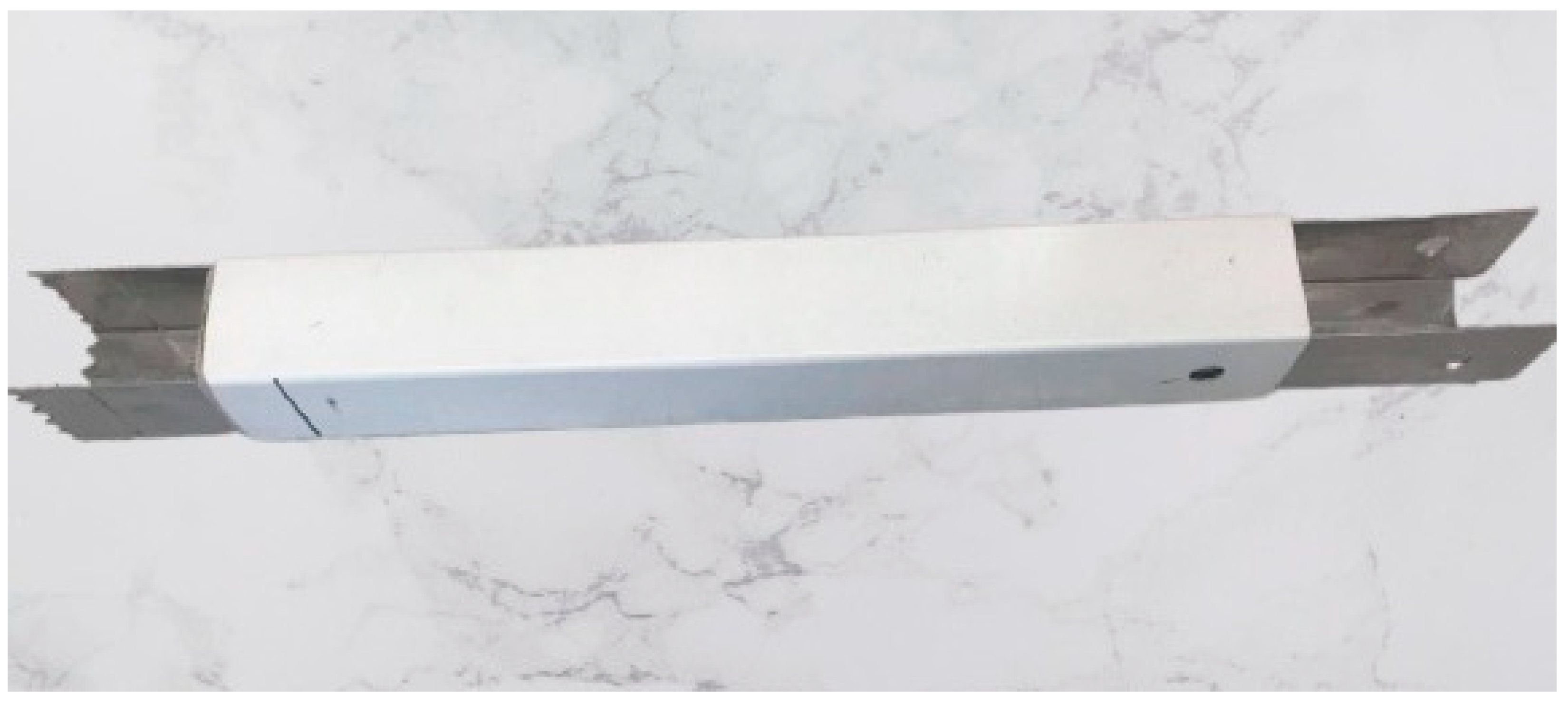
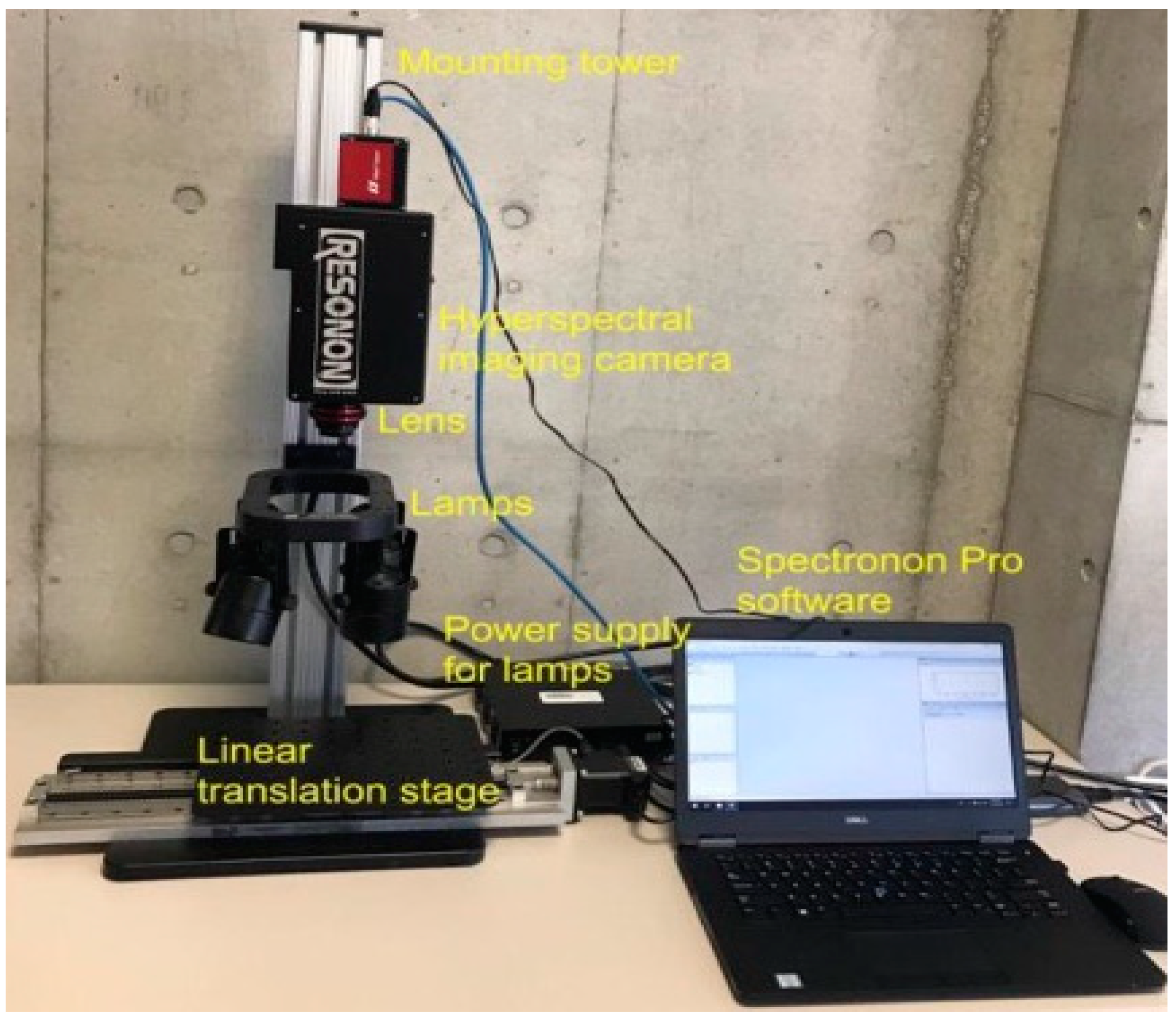
Two types of instruments were used to generate the calibration and validation database. Snow samples were collected using a rectangular core sampler designed and built by INRS’s remote sensing team (Figure 2), and optical properties were measured using a proximal acquisition station (Figure 3). The data acquired with these two instruments were collected at the same place and time.
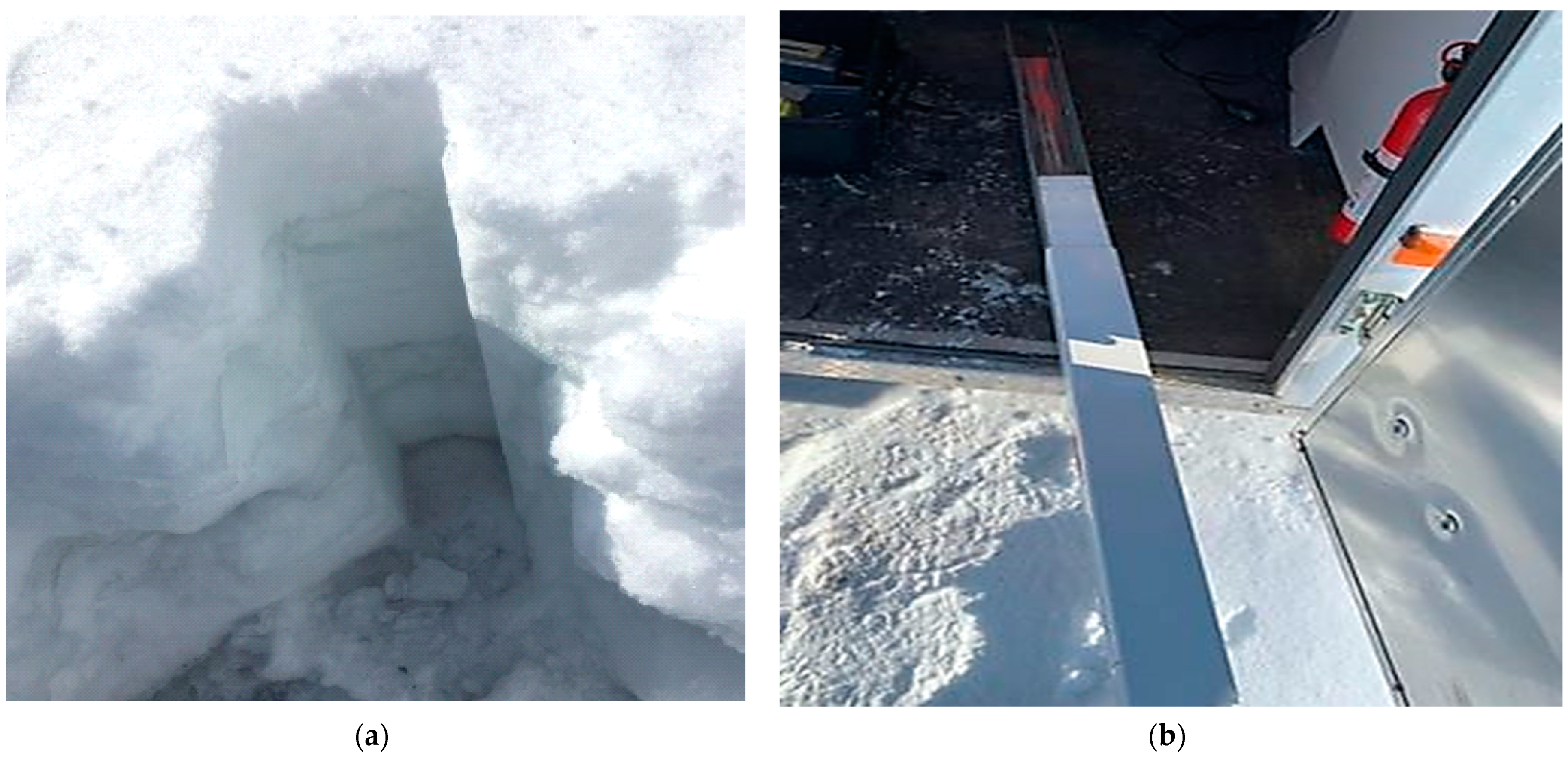
The rectangular core sampler (or corer) was used to extract the vertical stratigraphy of the snowpack (Figure 4a). The corer is composed of a metallic inner component and a plastic cover with a triangular sawtooth cutting part at the end. This design allows the extraction of the vertical profile of the snowpack with all its metamorphosed variants and no loss of snow (Figure 4b). The corer is graduated to measure the height (cm) of the profile and to differentiate the homogeneous layers composing the vertical profile.
The proximal acquisition station used in this work is equipped with a hyperspectral camera (PIKA NIR from RESONON Company) boarded on a linear translation plate which allows for fast acquisition of spectral data (Figure 3). The camera measures the NIR spectral reflectance for wavelengths between 900 nm and 1700 nm with a spectral resolution of 5.5 nm for 148 spectral bands. The station also contains a halogen lighting system, a mounting tower, a mobile platform, a data acquisition software (Spectronon Pro by Resonon Inc., Bozeman, MT, USA), and proximal acquisition lenses (Figure 3).
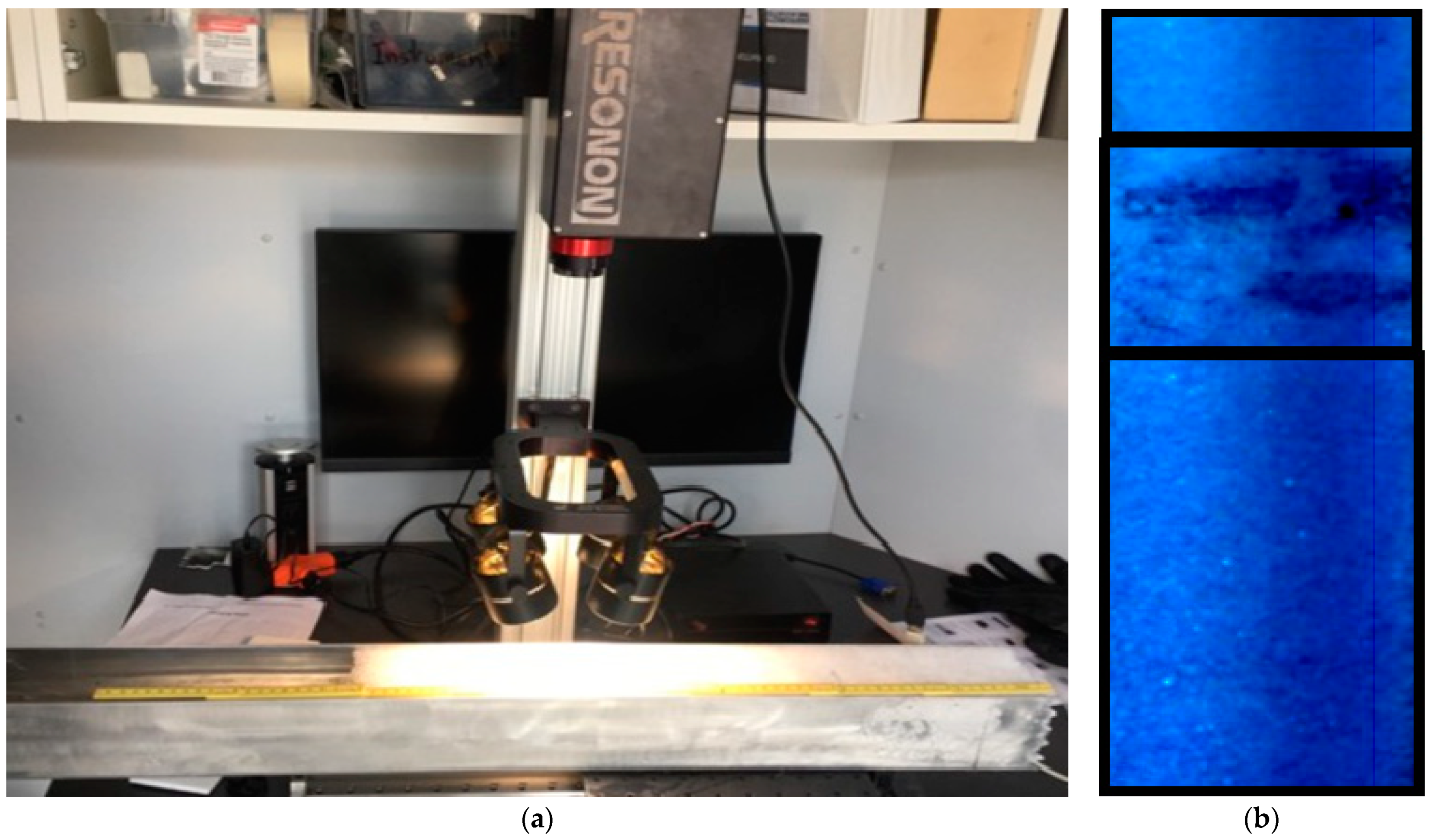
The snow sample is collected by pushing the corer through the surface of the snowpack until the serrated cutting end reaches the ground. This ensures the recovery of both surface snow and snow from deeper layers (Figure 4a). Once the snow is extracted (Figure 4b), it is scanned with the NIR hyperspectral camera (Figure 5a), and the generated image is analyzed by the Spectronon Pro software (Figure 5b) [39]. The latter identifies the homogeneous layers previously measured in the field and analyzes the spectral responses of each one. After this, each homogeneous layer is carefully removed from the corer, and its physical properties are characterized. The layers are then classified according to the International classification of seasonal ground snow [40]. To do so, the size and type of snow grains are identified using a millimeter grid map and observed with a magnifying glass (10×). Finally, the isolated layers are weighed, and the density of each one is calculated [39]. All observations and measurements were performed by the same person to ensure consistency.
2.3. Methodological Approach
The methodological approach adopted is based on three main phases that are summarized in the flow chart illustrated in Figure 6:
- ❖
- The calibration of the classifier and the specific estimation of the HM
The calibration was carried out in two steps: (1) Development of a machine learning-based algorithms using CART (classification and regression tree) method to discriminate between three different snow classes (WMM, MHM, and HVM) based on the NIR spectral data; The CART algorithm is a tree-based decision process. It uses a training sample set composed of a historical data set with pre-assigned classes for all observations (density in our case) and splitting variables (spectral bands in our case). These decision trees are spectrally based thresholds that are then used to classify new data [41]. And (2) Subdivision of the calibration database, based on the previously developed classifier, into three sub-data sets. These sub-data sets were then used to train three specific estimators. For each specific estimator, all possible band ratios were first calculated and correlated with the snow density values. The correlation coefficients were then stored in a coefficient correlation matrix. The most highly correlated band ratios (R2 > 0.5) were then integrated into a stepwise algorithm to train the calibration function. This exercise was also applied to the band differences and the normalized differences independently. Whether based on ratios, differences, or normalized differences, the spectral index most highly correlated with each specific estimator was retained at the end of the calibration step.
- ❖
- Evaluation of the specific estimators using the leave-one-out cross-validation (LOOCV) algorithm [42];
The specific estimators were assessed using the LOOCV method. This method consists of temporarily removing an entry from the database and using the rest of the database as calibration data, and then estimating the density of the removed measurement. This operation is repeated for the entire database. The main objective of this step was to calculate the relative bias of each specific estimator.
- ❖
- HM evaluation using independent data selected using the systematic split validation (SSV) technique.
Firstly, 25% of the data was removed from the initial database prior to the calibration of the MH for independent validation purposes. The validation data were systematically selected (the 4th data entries starting with low to high-density values) and set aside. This technique is known as systematic split validation (SSV). The remaining data (calibration database) was used to train the HM. Finally, to assess the overall accuracy of the HM, the independent dataset (the 25% removed by the SSV technique) was used. It is important to note, however, that it was necessary to go through both calibration steps to accurately assess the MH. Each sample was first assigned to one of three snow classes using the HM classifier. The snow density was then estimated using the specific estimator corresponding to the pre-assigned class.
Four statistical indices were used to assess both the specific estimators and the HM, which are presented in Equations (1)–(4). These are the coefficient of determination (R2), defined as the squared value of the correlation coefficient, the root means square error (RMSE), the bias (BIAS), and the Nash-criterion (NASH). The NASH criterion [43] compares the values estimated by the model to the mean in-situ measurements, yielding a result between −∞ and 1.0 (inclusive). A negative NASH result means that it would be preferable to use the mean in-situ measurements rather than the model estimates, whereas values between 0.0 and 0.6 are generally considered acceptable levels of model performance. Model performance is satisfactory for values above 0.8, and the model is perfect when NASH = 1.0. The mathematical equations for these indices are as follows:
where: n is the size of the dataset, M and Es are the measured and estimated density values, and are the means of the measured and estimated values.
3. Results and Discussion
3.1. Descriptive Analysis of Data
Domine, Taillandier, and Simpson [36] proposed snow grain size parameterizations based on snow density and grain shape, grouping snow samples into three main types (fresh, recent, and old). Based on this principle, we treated the snowpack as a succession of layers. Each layer is characterized by its own physical properties depending on its history and maturation stage of transformation [44]. The layers are reported in Table 1 and are grouped by grain size, grain type, and layer density, as defined by Pahaut [45]. Based on these physical properties, each layer of snow has been assigned to one of three general predefined snow classes (WMM, MHM, and HVM) following the classification of Pahaut [45] and the International classification of seasonal ground snow [40] protocols. For inventory purposes, a description and pictures of snow grains with their corresponding dates were taken for each layer. These were used later as real in-situ data when verification was needed.
A database of 114 layers was established (Table 1). Snow densities varied between 100 kg m−3 and 650 kg m−3, with an average of 320 kg m−3 and a standard deviation of 130 kg·m−3. According to the Pahaut [45] classification, 19 layers (samples) were identified as WMM, 59 as MHM, and 36 as HVM. For WMM, MHM, and HVM, respectively, the minima were 100 kg m−3, 150 kg m−3, and 350 kg m−3; the maxima were 250 kg m−3, 400 kg m−3, and 650 kg m−3; the means were 170 kg m−3, 280 kg m−3, and 460 kg m−3; the standard deviations were 50 kg m−3, 78 kg m−3, and 82 kg m−3. In Table 1, we consider newly deposited snow on the snowpack to be characterized by small grain size and low density, while moderately and heavily metamorphosed snow was characterized by moderate and large grain size and density, respectively. The smaller number of layers in the WMM class is due to the difficulty of isolating this type of layer because weakly metamorphosed snow is very light and often thin.
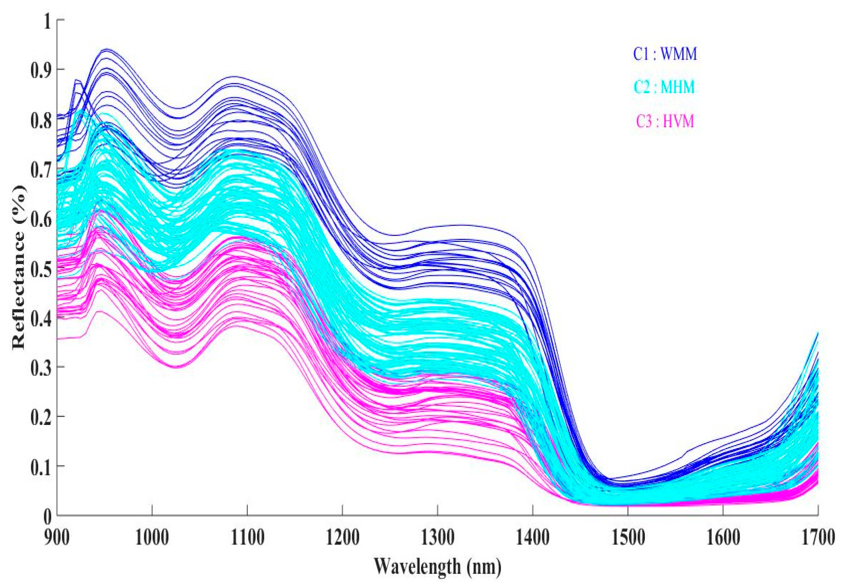
Figure 7 shows the measured NIR reflectance spectrum of the 114 snow samples (layers) extracted from twenty-four snow cores (all field campaigns included). The shape of the spectral reflectance changes as a function of the physical properties of the snow (density, grain size, and grain shape), which depends on the state of transformation by the metamorphosis of each layer. In fact, each layer is characterized by its own spectral reflectance, which is characterized by the degree of reflection, absorption, and transmission in each wavelength of the NIR spectrum. This results in similarities between the reflectance spectra of layers with similar chemical composition and physical characteristics [46]. This is translated by a decrease of reflectance as the snow layer ages; WMM, MHM, and HVM are colored dark blue, sky blue, and pink, respectively. These findings show that it is possible to discriminate between the three predefined classes based only on the reflectance spectra of the layers.
3.2. Statistical Dependence between Density and Spectral Reflectance
Previous works have failed to establish a strong correlation between snow density and reflectance, neither in the visible [37,47] nor in the NIR [36,37,47] parts of the spectrum. The same poor correlations (maximum correlation of R2 = 0.53) were also found in this study when using single bands, as shown by the graphical correlogram shown in Figure 8a. The R2 is also presented as a correlation matrix using three spectral indices: normalized band differences (Figure 8b), band ratios (Figure 8c), and band differences (Figure 8d). The accuracy was relatively increased, and the results are consistent with other published works [33,34]. The best correlation for the normalized band differences, band ratios, and band differences was found with the spectral ranges of 1034–1051 nm (R2 = 0.64), 1205–1309 nm (R2 = 0.63), and 1644–1655 nm (R2 = 0.56), respectively. The above results affirmed that the correlation between the snow density and the spectral indices is relatively moderate (R2 =< 0.64).
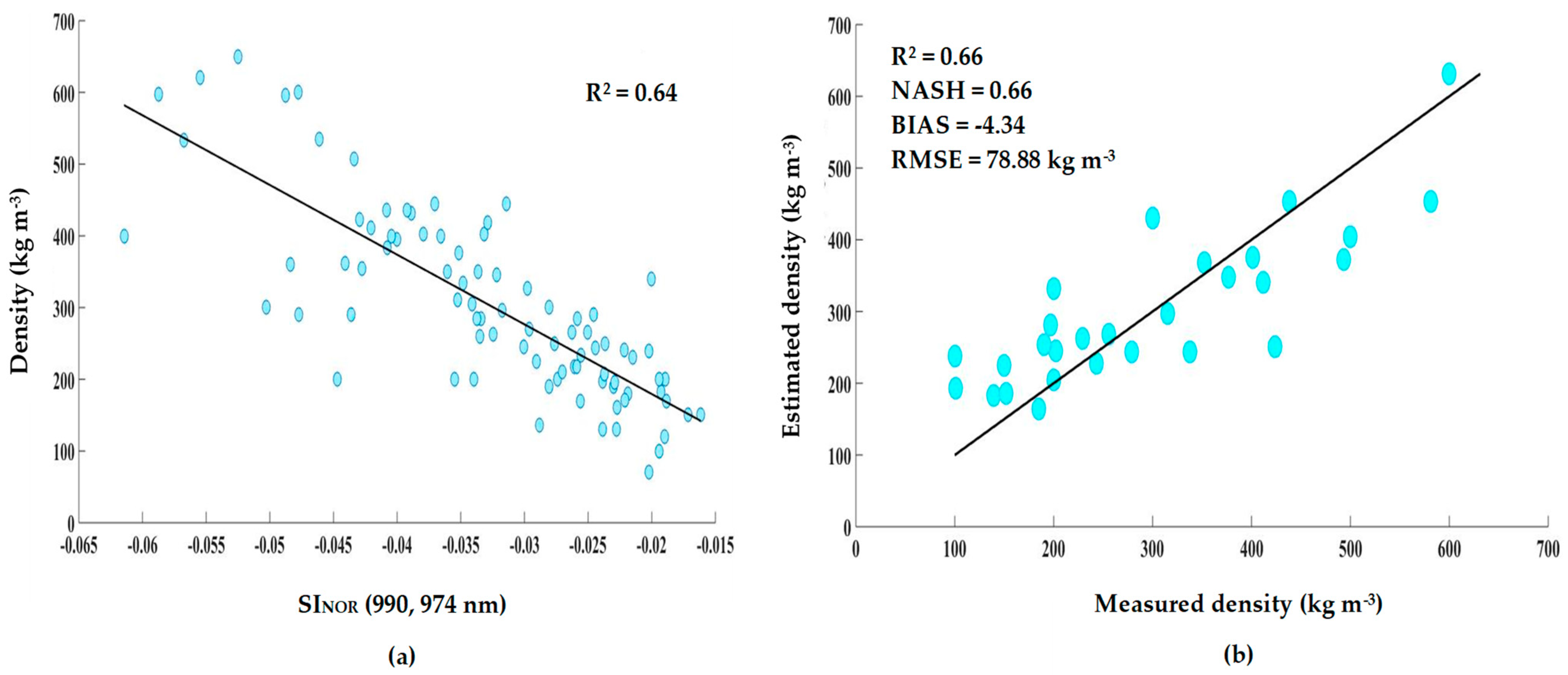
Based on the above results, it was decided to go through the calibration and validation steps with the highest correlation, which was the normalized band differences. It is important to note, however, that these results are based on 75% of the initial database, as the remaining 25% was utilized for validation purposes. In order to avoid autocorrelation between independent variables, it was decided to correlate only the bands with the best associations (here called neo-variables for simplicity) with snow density. The result is shown in Figure 9a. The density is sensitive to wavelengths 974 nm and 990 nm, with an R2 of 0.64. When the model was validated using the independent data set (25% removed), all statistical indices showed moderate accuracy in estimating snow density, particularly R2 and Nash (R2 = Nash = 0.66; Figure 9b).
The aforementioned analysis confirms that the reciprocal correlation between the spectral reflectance in the NIR and snow density is probably the result of other changes in the aging process, such as temperature, day length, radiation, etc. [35]. Indeed, despite the strong correlation between the decrease in reflectance and the increase in density (Figure 7), it is difficult to evaluate the extent to which the decrease should be attributed to the underlying physical cause of densification, and this is where the difficulty of experimentally relating spectral reflectance (using single bands or based on neo-variables) to snow density lies.
3.3. Calibration of the Hybrid Model
3.3.1. HM Classifier Calibration
Although several density models exist, most assume that snow density can be modeled using a single function (such as the one developed above). The use of a single function, even if it is multi-varied, is still confronted with the inherent surjective relationship between snow density and spectral reflectance. Therefore, replacing the surjective relation with several bijective relations could be the answer to increase the accuracy of snow density modeling. This could be achieved by establishing a strong correlation between the decrease in reflectance and the increase in density. To validate this hypothesis, a classification algorithm was applied to the calibration database to discriminate between the three predefined snow classes (WMM, MHM, and HVM) based on spectral reflectance and, hopefully, to increase the relationship between snow density and spectral reflectance in each class; converting this surjective relationship into three bijective relationships.
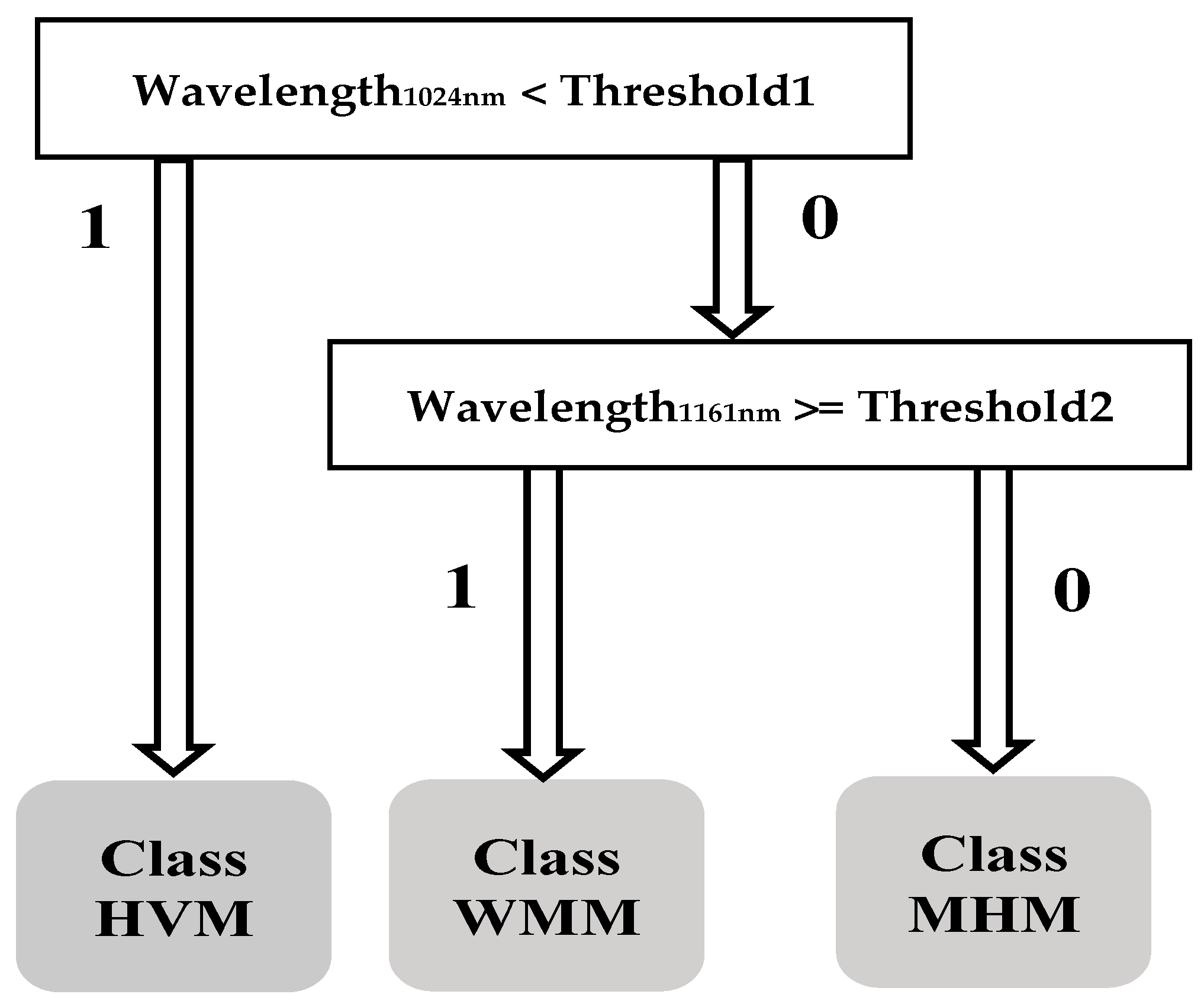
The results of in-situ measurement classification, presented in Table 1, were used to develop the HM’s classifier using the CART algorithm. CART results are represented in the form of an intuitive illustration (Figure 10). Two wavelengths (1024 nm and 1161 nm) were selected as the best classifier thresholds, which allowed us to calibrate the classifier of the HM. Dozier and Painter [35] demonstrated that the spectral reflectance of snow displays an ice absorption feature centered at 1030 nm that can be used to estimate snow grain size from hyperspectral data. Roy et al. [48] used this ice absorption feature to distinguish natural snow from compacted or metamorphosed snow. The wavelengths identified by the CART are coherent with the works cited above. According to Figure 10, the band centered at 1024 nm allows to differentiate between the highly metamorphosed snow class (composed of snow grains of size > 2 mm) and the other two classes of weakly and moderately metamorphosed snow and the band centered at 1161 nm allows to discriminate between the moderately and weakly metamorphosed snow (composed of snow grains of size < 1 mm).
3.3.2. Calibration of the Specific Models
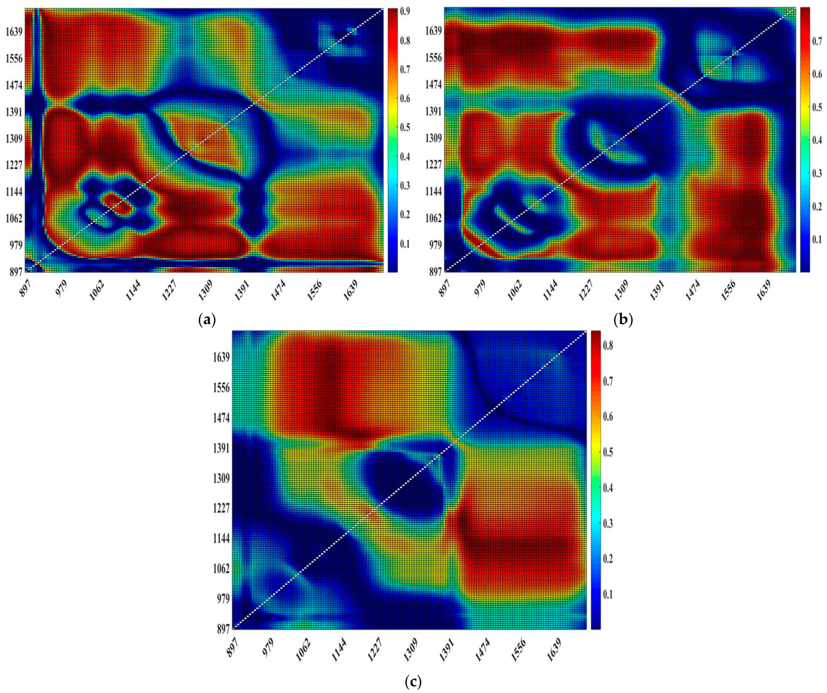
The calibrated classifier was then used to subdivide the calibration database into three subclasses based on spectra. Fifteen samples were used as a training dataset for the WMM class, 44 for the MHM class, and 27 for the HVM class. Each subclass dataset was thereafter used to calibrate its own specific estimator. The calibration step was performed using multivariate stepwise regression in which the independent variables were selected using an automatic procedure that typically followed a sequence of F-tests. Stepwise regression was used in a direct selection mode, starting with none of the variables in the model, testing them one by one, and including only statistically significant variables [49]. For comparison purposes, the calibration and validation steps were performed exactly as indicated in the section above. However, only significant results are presented to alleviate the text. As expected, the correlation between snow density and spectral reflectance was higher when each class was considered separately. Snow density showed a wider range of sensitivity to neo-variables, which was different for band differences and normalized band differences, depending on the class (Figure 11). These findings support the assumption that destroying the surjective relationship could lead to the creation of a bijective relationship in each class and consequently enhancing the model’s accuracy. Also, the highest correlations are not necessarily centered at the same wavelength for each class. This is a demonstration that each class has its own response to the spectral reflectance and the optimal wavelengths to detect snow density shift depending on the class. This is to be expected since the density depends on the grain size, the grain type, and the liquid water content. In addition, it is known that water strongly absorbs in the NIR [34]. Hence, the higher the water content of snow, the smaller the returned signal (and vice versa).
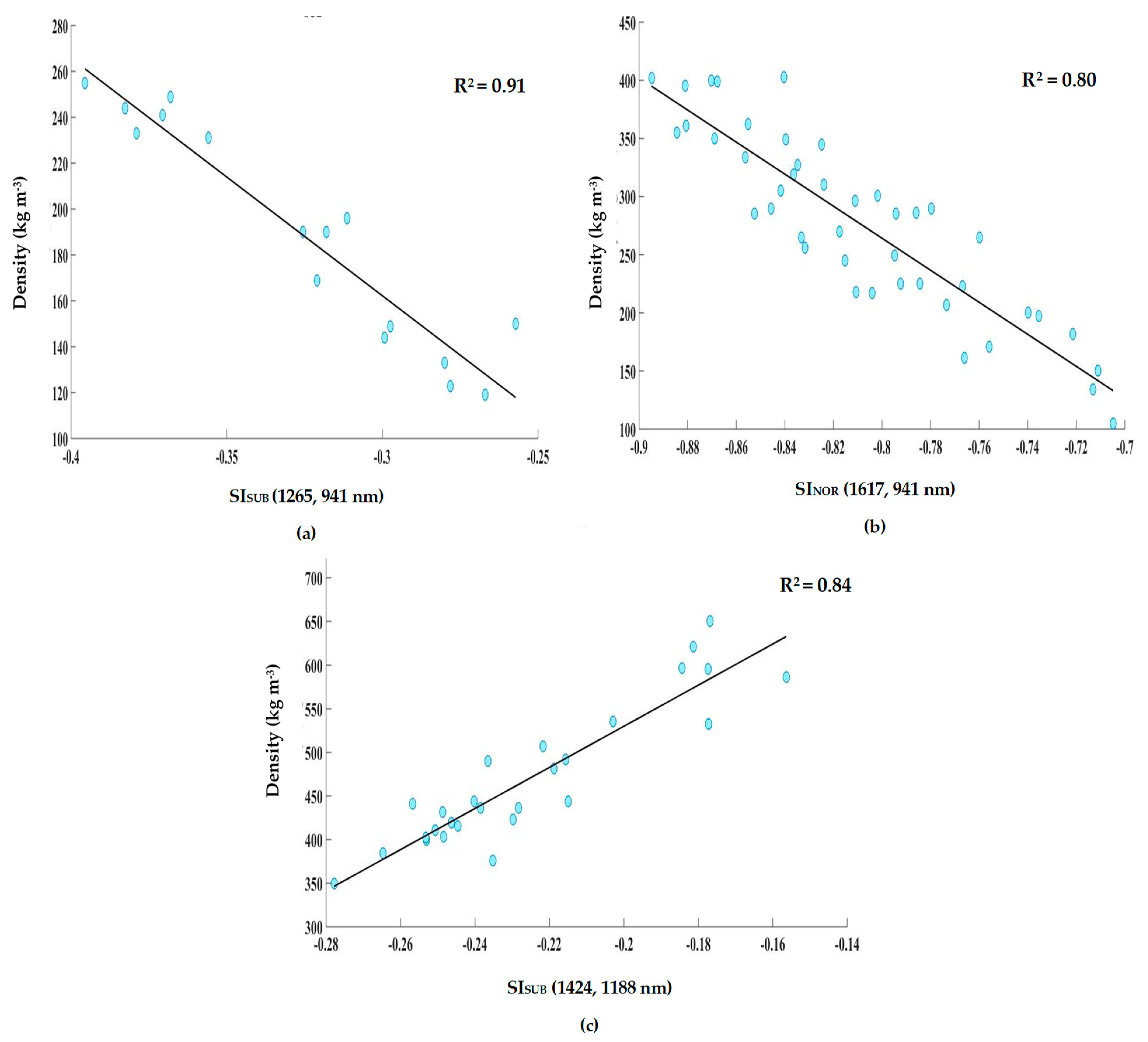
Results of the stepwise algorithm are presented in Figure 12. The three snow classes were linearly correlated, and the calibration functions were univariate (Table 2). The neo-variable retained for the WMM class was the difference between 1265 nm and 941 nm wavelengths (referred to as the spectral index of subtraction; SISUB) with an R2 of 0.91. The neo-variable retained for the MHM class was the normalized difference between 1617 nm and 941 nm wavelengths (referred here as the spectral index of normalized difference; SINOR) with an R2 of 0.80. The neo-variable retained for the HVM class was also the difference between 1424 nm and 1188 nm wavelength (SISUB) with an R2 of 0.84.
These results are coherent with other works. For example, Negi et al. [46] found that for changes in liquid water content, grain size, and metamorphosis level (aging) of snow, the maximum spectral variations are observed around the shorter wavelengths of the NIR spectrum. Gallet et al. [50] used the NIR spectrum to determine the size of snow grains. They found that the band centered at 1310 nm, which corresponds to the central part of the NIR spectrum, is sensitive to small snow grains, which are usually of low to medium density, and that the band centered at 1550 nm, which corresponds to the higher part of the NIR spectrum, is sensitive to large snow grains, where the snow is generally denser. The strong correlation between in situ density measurements and spectral indices (R2 > 0.80) for all three specific estimators illustrates the importance of dividing the input data into several classes of snow (three in this study), based on a certain degree of aging. For all specific estimators, the estimation of snow density was limited to short (941 nm, 1265 nm, and 1188 nm) and long (1424 nm and 1617 nm) NIR wavelengths, which are the spectral regions most sensitive to the physical properties of snow. The mathematical expressions of the three specific estimators are summarized in Table 2.
3.4. Evaluation and Validation of the Hybrid Model
3.4.1. Evaluation of the Specific Estimators Using the LOOCV Algorithm
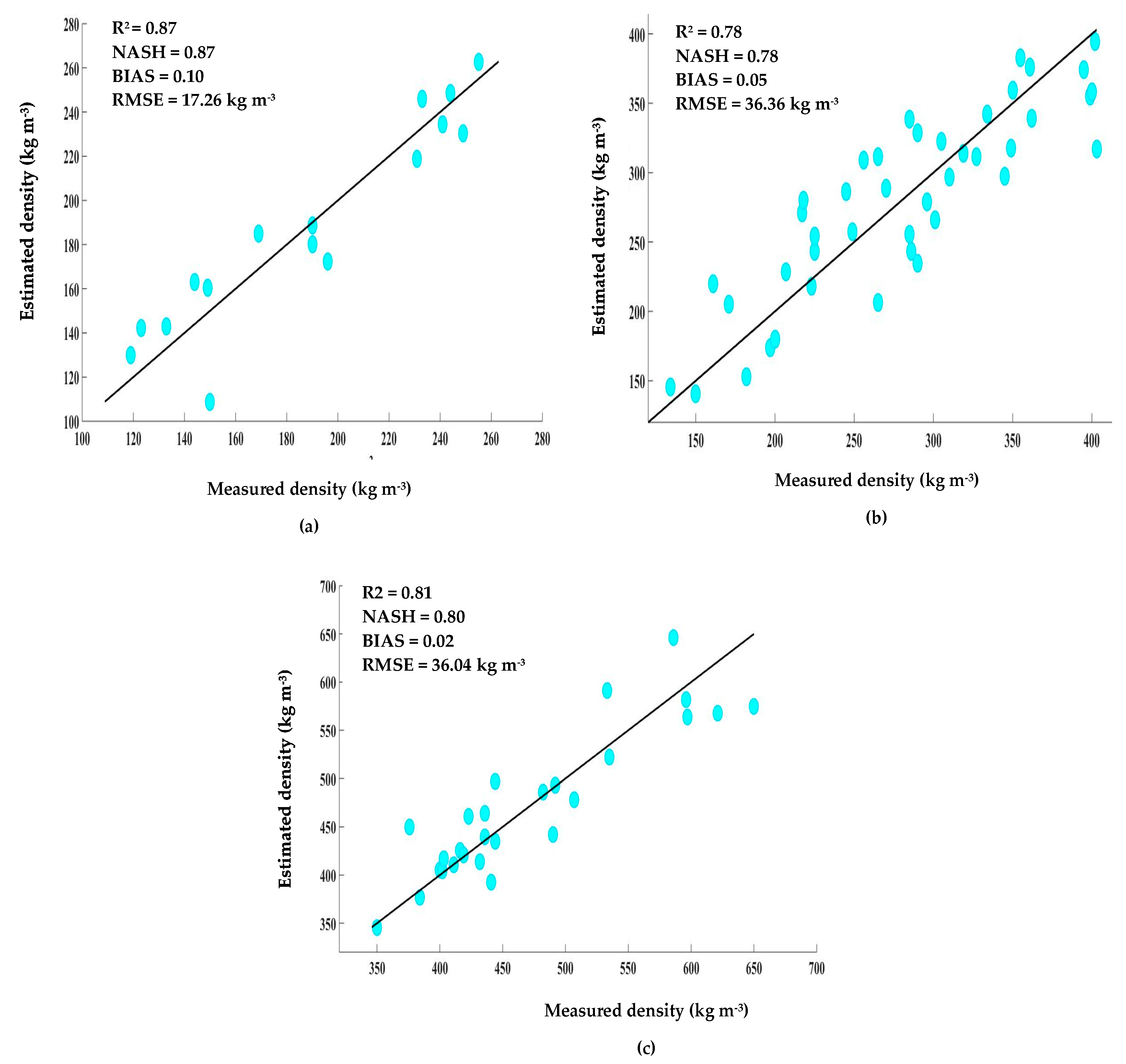
The LOOCV is a technique that consists of temporarily removing certain entries from a database and using the rest as calibration data, and then estimating the value of the removed entry. This operation is repeated for the entire database, resulting in an estimate for the entire database, hence allowing the comparison between estimated and measured values (Equations (1)–(4)). Figure 13 shows the LOOCV results of the three specific estimators. The estimators’ ability to model snow density is satisfactory for the WMM, MHM, and HVM classes with a respective value of R2 of 0.87, 0.78, and 0.81. The RMSE of the three specific estimators are 17.26 kg m−3, 36.36 kg m−3, and 36.04 kg m−3, respectively, for the WMM, MHM, and HVM classes, which is satisfactory as well. The BIAS is positive for all three classes.
The LOOCV was not intended to evaluate the HM’s snow density estimates, and its main objective was to quantify the BIAS of each specific estimator. In fact, each modeling process is tainted by two sources of error: (1) a random error quantified by the RMSE, and (2) a systematic error quantified by the BIAS. The first one is not correctable, but the second one is adjustable and can be removed/added to the estimates during the modeling process. This part of the study was aimed at quantifying the systematic error and using it to adjust the final model.
3.4.2. Evaluation of the Hybrid Model Using SSV
The HM was evaluated using independent data. However, it is important to note that in order to use SSV data for validation, it was necessary to go through all the calibration steps:
- ❖
- Assign a given class using the HM classifier;
- ❖
- Estimate the density using the specific estimators corresponding to the preassigned class;
- ❖
- Correct the estimates’ BIAS;
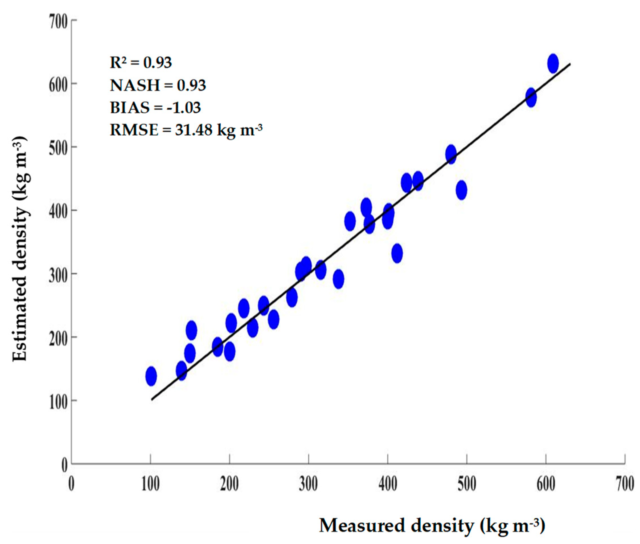
Figure 14 shows the results of the evaluation of the HM’s ability to estimate the snow density. The points are well distributed along the 1:1 line, from very low to high-density values. The value of the NASH index (R2 = 0.93) highlights the good performance of the model. A satisfactory value of RMSE (31.48 kg m−3) is also achieved. As these results show, the performance of the HM is satisfactory, especially with a dataset covering a three-winter period. This period may seem long, but with global warming and climate change affecting climatic systems around the world, the seasonal snowpack is expected to also be changing from year to year. This is why finding an independent dataset to assess the performance of the HM was very challenging. Despite this, the evaluation shows that the HM accurately modeled the snow density using optical data. Contrary to previous studies claiming that there is no strong correlation between spectral reflectance and snow density, this study has shown that it is possible to estimate snow density if the right modeling strategy is found.
The implementation of the approach developed in this work can constitute a real advance in the determination and monitoring of the various processes that lead to the continuous evolution and regular monitoring of the density of the seasonal snow cover. The results also highlight many of the difficulties inherent in measuring the density of snow on the ground, which presents considerable lateral variability (accumulation of layers of different densities). This large lateral variability is common to all snowpacks, and measuring only the average density of the latter does not represent the overall vertical profile. The approach described here, when fully matured, provides a means of obtaining the necessary data for these purposes.
4. Conclusions
The objective of this study was to test the performance of a hybrid model (HM) designed to estimate the density of the seasonal snowpack using hyperspectral NIR imaging (900–1700 nm) at a spectral resolution of 5.5 nm. The hybrid model is a combination of a classifier and three specific estimators (weakly to moderately metamorphosed snow (WMM), moderately to highly metamorphosed snow (MHM), and highly to very highly metamorphosed snow (HVM)). The hybrid model was evaluated at two levels: using the leave-one-out cross-validation (LOOCV) algorithm and using the systematic division validation technique (SSV). The LOOCV technique was used to assess the three specific estimators, and the SSV data were used to assess the performance of the HM.
The calibration step, based on a stepwise multivariate regression, showed that the three classes of snow are sensitive to different regions of the NIR spectrum, limited to the short and long wavelengths. The WMM was sensitive to the wavelengths at 1265 nm and 941 nm, the MHM was sensitive to wavelengths at 1617 nm and 941 nm, and the HVM was sensitive to wavelengths at 1424 nm and 1188 nm. The LOOCV technique highlighted that the specific estimators of all classes tend to slightly overestimate the snow density (BIAS < 0.1 kg·m−3). When the HM was challenged with SSV data, the modeling results were satisfactory with an R2 = Nash = 0.93, and the snow density was slightly underestimated (BIAS = 1.03 kg·m−3).
The objective of this study was to develop a method based on the optical properties of snow to be used conjointly with conventional density measurement methods with the aim of alleviating field operations. The critical step in estimating snow density using the HM is the selection of the final specific estimator. Indeed, classification algorithms (such as CART) are known to be local and unstable. This instability can significantly affect the accuracy of the density using the specific estimators of the HM. In other words, for an ideal modeling process using the HM, the sample to be modeled must be well classified so that the specific estimator corresponding to that class is used for optimal density estimation. Otherwise, a wrong specific estimator will be selected, and consequently, the estimation will not be optimal, which could affect the accuracy. For example, for a measured density of 581 kg m−3 (classified as HVM), the relative errors vary by 5%, 39%, and 75% when estimated using specific estimators of HVM, MHM, and WMM, respectively. On the other hand, another obstacle associated with this method is the correct selection of homogeneous snow layers in the field and on the recovered hyperspectral image. For this reason, additional field campaigns need to be conducted to collect more data to overcome this weakness and allow proper field implementation. The HM provides an improved tool to monitor the evolution of seasonal snowpacks, with a satisfactory level of performance even for low to moderate snow densities. We conclude that our results are an important first step toward the development of an effective method for continuous monitoring of snow density profiles in the field.
Author Contributions
Conceptualization, M.K.E.O. and K.C.; methodology, M.K.E.O., A.E.A. and K.C.; writing—original draft preparation, M.K.E.O.; writing—review and editing, M.K.E.O., A.E.A. and M.B.; supervision, K.C. and A.E.A. All authors have read and agreed to the published version of the manuscript.
Funding
This research received no external funding.
Institutional Review Board Statement
Not applicable.
Informed Consent Statement
Not applicable.
Data Availability Statement
Not applicable.
Acknowledgments
Many people have reviewed and commented on the drafts of this document. The comments of Anas El Alem, Monique Bernier were particularly appreciated. Karem Chokmani’s encouragements were very helpful, as was his valuable guidance. The preparation of this manuscript, the retrieval, measurement and photography of snow profiles and my work on snow metamorphism have been supported over the years in developing this work. Many thanks to Sophie Roberge and David Ethier for their efficient coordination of the field campaign. Thanks also to Jimmy Poulin, Hachem Agili and Rachid Lhissou for their help and suggestions.
Conflicts of Interest
The authors declare that they are submitting the manuscript to the journal without any known conflict of interest.
References
- Kropacek, J.; Feng, C.; Alle, M.; Kang, S.; Hochschild, V. Temporal and spatial aspects of snow distribution in the Nam Co Basin on the Tibetan Plateau from MODIS data. Remote Sens. 2010, 2, 2700–2712. [Google Scholar] [CrossRef] [Green Version]
- Marbouty, D. Les propriétés physiques de la neige. Houille Blanche 1984, 557–567. [Google Scholar] [CrossRef] [Green Version]
- Davis, R.; Pangburn, T.; Daly, S.; Ochs, E.; Hardy, J.; Bryant, E.; Pugner, P. Can satellite snow maps, ground measurements, and modeling improve water management and control in the Kings River Basin, California. In Proceedings of the Efforts toward finding the answer—67th Annual Western Snow Conference, South Lake Tahoe, CA, USA, 19–22 April 1999; pp. 54–61. [Google Scholar]
- Fassnacht, S.; Helfrich, S.; Lampkin, D.; Dressler, K.; Bales, R.; Halper, E.; Reigle, D.; Imam, B. Snowpack modelling of the Salt Basin with water management implications. In Proceedings of the Annual Western Snow Conference, Sun Valley, ID, USA, 17–19 April 2001; pp. 65–76. [Google Scholar]
- Brown, R.; Armstrong, R. Snow-cover data: Measurement, products, and sources. In Snow and Climate; Armstrong, R.L., Brun, E., Eds.; Cambridge University Press: Cambridge, UK, 2008; pp. 181–216. [Google Scholar]
- Dutra, E.; Viterbo, P.; Miranda, P.M.; Balsamo, G. Complexity of snow schemes in a climate model and its impact on surface energy and hydrology. J. Hydrometeorol. 2012, 13, 521–538. [Google Scholar] [CrossRef]
- Castebrunet, H.; Eckert, N.; Giraud, G.; Durand, Y.; Morin, S. Projected changes of snow conditions and avalanche activity in a warming climate: The French Alps over the 2020–2050 and 2070–2100 periods. Cryosphere 2014, 8, 1673–1697. [Google Scholar] [CrossRef] [Green Version]
- Lehning, M.; Bartelt, P.; Brown, B.; Russi, T.; Stöckli, U.; Zimmerli, M. SNOWPACK model calculations for avalanche warning based upon a new network of weather and snow stations. Cold Reg. Sci. Technol. 1999, 30, 145–157. [Google Scholar] [CrossRef]
- Langham, E.J. Physics and properties of snowcover. In Handbook of Snow, Principles, Processes, Management and Use; Gray, D.M., Male, D.H., Eds.; Pergamon Press: Toronto, ON, USA, 1981; pp. 275–337. [Google Scholar]
- Pomeroy, J.W.; Hanson, S.; Faria, D. Small-scale variation in snowmelt energy in a boreal forest: An additional factor controlling depletion of snow cover. In Proceedings of the Eastern Snow Conference, Ottawa, ON, Canada, 17–19 May 2001; pp. 85–96. [Google Scholar]
- Roy, V.; Goïta, K.; Royer, A.; Walker, A.E.; Goodison, B.E. Snow water equivalent retrieval in a Canadian boreal environment from microwave measurements using the HUT snow emission model. IEEE Trans. Geosci. Remote Sens. 2004, 42, 1850–1859. [Google Scholar] [CrossRef]
- Sturm, M.; Taras, B.; Liston, G.E.; Derksen, C.; Jonas, T.; Lea, J. Estimating snow water equivalent using snow depth data and climate classes. J. Hydrometeorol. 2010, 11, 1380–1394. [Google Scholar] [CrossRef]
- Farnes, P.; Goodison, B.; Peterson, N.; Richards, R. Proposed metric snow samplers. In Proceedings of the 48th Western Snow Conference, Laramie, WY, USA, 15–17 April 1980; pp. 107–119. [Google Scholar]
- Farnes, P. Criteria for determining mountain snow pillow sites. In Proceedings of the 35th Western Snow Conference, Boise, ID, USA, 18–20 April 1967; pp. 59–62. [Google Scholar]
- Kinar, N.; Pomeroy, J. Measurement of the physical properties of the snowpack. Rev. Geophys. 2015, 53, 481–544. [Google Scholar] [CrossRef]
- Zuanon, N. IceCube, a portable and reliable instruments for snow specific surface area measurement in the field. In Proceedings of the International Snow Science Workshop Grenoble-Chamonix Mont-Blance—2013 Proceedings, Grenoble, France, 7–11 October 2013; pp. 1020–1023. [Google Scholar]
- Wright, M.; Kavanaugh, J.; Labine, C. Performance analysis of GMON3 snow water equivalency sensor. In Proceedings of the Western Snow Conference, Stateline, NV, USA, 18–21 April 2011; pp. 105–108. [Google Scholar]
- Cui, Y.; Xiong, C.; Lemmetyinen, J.; Shi, J.; Jiang, L.; Peng, B.; Li, H.; Zhao, T.; Ji, D.; Hu, T. Estimating snow water equivalent with backscattering at X and Ku band based on absorption loss. Remote Sens. 2016, 8, 505. [Google Scholar] [CrossRef] [Green Version]
- Negi, H.; Jassar, H.; Saravana, G.; Thakur, N.; Snehmani; Ganju, A. Snow-cover characteristics using Hyperion data for the Himalayan region. Int. J. Remote Sens. 2013, 34, 2140–2161. [Google Scholar] [CrossRef]
- Gergely, M.; Schneebeli, M.; Roth, K. First experiments to determine snow density from diffuse near-infrared transmittance. Cold Reg. Sci. Technol. 2010, 64, 81–86. [Google Scholar] [CrossRef]
- Chauchard, F.; Cogdill, R.; Roussel, S.; Roger, J.; Bellon-Maurel, V. Application of LS-SVM to non-linear phenomena in NIR spectroscopy: Development of a robust and portable sensor for acidity prediction in grapes. Chemom. Intell. Lab. Syst. 2004, 71, 141–150. [Google Scholar] [CrossRef] [Green Version]
- Osborne, B.G. Near-infrared spectroscopy in food analysis. In Encyclopedia of Analytical Chemistry: Applications, Theory and Instrumentation; John Wiley and Sons: Hoboken, NJ, USA, 2006. [Google Scholar]
- Lu, G.; Fei, B. Medical hyperspectral imaging: A review. J. Biomed. Opt. 2014, 19, 010901. [Google Scholar] [CrossRef]
- Gallet, J.-C. La Neige du Plateau Antarctique. Surface Spécifique et Applications. Ph.D. Thesis, Université Joseph-Fourier-Grenoble I, Saint-Martin-d’Hères, France, 2010. [Google Scholar]
- ElMasry, G.; Sun, D.-W.; Allen, P. Near-infrared hyperspectral imaging for predicting colour, pH and tenderness of fresh beef. J. Food Eng. 2012, 110, 127–140. [Google Scholar] [CrossRef]
- Lorente, D.; Aleixos, N.; Gómez-Sanchis, J.; Cubero, S.; García-Navarrete, O.L.; Blasco, J. Recent advances and applications of hyperspectral imaging for fruit and vegetable quality assessment. Food Bioprocess Technol. 2012, 5, 1121–1142. [Google Scholar] [CrossRef]
- Haq, M.A.; Ghosh, A.; Rahaman, G.; Baral, P. Artificial neural network-based modeling of snow properties using field data and hyperspectral imagery. Nat. Resour. Model. 2019, 32, e12229. [Google Scholar] [CrossRef]
- Nolin, A.W.; Dozier, J. A hyperspectral method for remotely sensing the grain size of snow. Remote Sens. Environ. 2000, 74, 207–216. [Google Scholar] [CrossRef]
- Negi, H.S.; Singh, S.; Kulkarni, A.; Semwal, B. Field-based spectral reflectance measurements of seasonal snow cover in the Indian Himalaya. Int. J. Remote Sens. 2010, 31, 2393–2417. [Google Scholar] [CrossRef]
- Kulkarni, A.; Srinivasulu, J.; Manjul, S.; Mathur, P. Field based spectral reflectance studies to develop NDSI method for snow cover monitoring. J. Indian Soc. Remote Sens. 2002, 30, 73–80. [Google Scholar] [CrossRef]
- Dozier, J. Spectral signature of alpine snow cover from the Landsat Thematic Mapper. Remote Sens. Environ. 1989, 28, 9–22. [Google Scholar] [CrossRef]
- Warren, S.G.; Wiscombe, W.J. A model for the spectral albedo of snow. II: Snow containing atmospheric aerosols. J. Atmos. Sci. 1980, 37, 2734–2745. [Google Scholar] [CrossRef]
- Eppanapelli, L.K.; Lintzén, N.; Casselgren, J.; Wåhlin, J. Estimation of liquid water content of snow surface by spectral reflectance. J. Cold Reg. Eng. 2018, 32, 05018001. [Google Scholar] [CrossRef]
- Warren, S.G.; Brandt, R.E. Optical constants of ice from the ultraviolet to the microwave: A revised compilation. J. Geophys. Res. Atmos. 2008, 113. [Google Scholar] [CrossRef]
- Dozier, J.; Painter, T.H. Multispectral and hyperspectral remote sensing of alpine snow properties. Annu. Rev. Earth Planet. Sci. 2004, 32, 465–494. [Google Scholar] [CrossRef] [Green Version]
- Domine, F.; Taillandier, A.S.; Simpson, W.R. A parameterization of the specific surface area of seasonal snow for field use and for models of snowpack evolution. J. Geophys. Res. Earth Surf. 2007, 112. [Google Scholar] [CrossRef]
- Li, H.; Wang, A.; Guan, D.; Jin, C.; Wu, J.; Yuan, F.; Shi, T. Empirical model development for ground snow sublimation beneath a temperate mixed forest in Changbai mountain. J. Hydrol. Eng. 2016, 21, 04016040. [Google Scholar] [CrossRef]
- Bohren, C.F.; Beschta, R.L. Snowpack albedo and snow density. Cold Reg. Sci. Technol. 1979, 1, 47–50. [Google Scholar] [CrossRef]
- El Oufir, M.K.; Chokmani, K.; El Alem, A.; Agili, H.; Bernier, M. Seasonal snowpack classification based on physical properties using near-infrared proximal hyperspectral data. Sensors 2021, 21, 5259. [Google Scholar] [CrossRef]
- Fierz, C.; Armstrong, R.L.; Durand, Y.; Etchevers, P.; Greene, E.; McClung, D.M.; Nishimura, K.; Satyawali, P.K.; Sokratov, S.A. The International Classification for Seasonal Snow on the Ground; UNESCO/IHP: Paris, France, 2009; Volume 25. [Google Scholar]
- Breiman, L.; Friedman, J.; Olshen, R.; Stone, C. Classification and Regression Trees; Wadsworth Statistics/Probability Series; Wadsworth: Monterey, CA, USA, 1984. [Google Scholar]
- Vehtari, A.; Gelman, A.; Gabry, J. Practical Bayesian model evaluation using leave-one-out cross-validation and WAIC. Stat. Comput. 2017, 27, 1413–1432. [Google Scholar] [CrossRef] [Green Version]
- Nash, J.E.; Sutcliffe, J.V. River flow forecasting through conceptual models part I—A discussion of principles. J. Hydrol. 1970, 10, 282–290. [Google Scholar] [CrossRef]
- Libois, Q. Evolution des propriétés physiques de neige de surface sur le plateau Antarctique. Observations et Modélisation du Transfert Radiatif et du Métamorphisme. Thèse de Doctorat, Université de Grenoble, Grenoble, France, 2014. [Google Scholar]
- Pahaut, E. Les Cristaux de Neige et Leurs Métamorphoses; Centre d’étude de la neige. St-martin d’hérés: Grenoble, France, 1975. [Google Scholar]
- ElMasry, G.; Sun, D.-w. Principles of hyperspectral imaging technology. In Hyperspectral Imaging for Food Quality Analysis and Control; Elsevier: Amsterdam, The Netherlands, 2010; pp. 3–43. [Google Scholar]
- Ling, F.; Zhang, T. A numerical model for surface energy balance and thermal regime of the active layer and permafrost containing unfrozen water. Cold Reg. Sci. Technol. 2004, 38, 1–15. [Google Scholar] [CrossRef]
- Roy, V.; Goita, K.; Granberg, H.; Royer, A. On the use of reflective hyperspectral remote sensing for the detection of compacted snow. In Proceedings of the Geoscience and Remote Sensing Symposium, 2006—IGARSS 2006, Denver, CO, USA, 31 July–4 August 2006; pp. 3263–3266. [Google Scholar]
- Wilkinson, L. Tests of significance in stepwise regression. Psychol. Bull. 1979, 86, 168. [Google Scholar] [CrossRef]
- Gallet, J.-C.; Domine, F.; Dumont, M. Measuring the specific surface area of wet snow using 1310 nm reflectance. Cryosphere 2014, 8, 1139–1148. [Google Scholar] [CrossRef] [Green Version]
Figure 1.
Geographic location of the sampling area in the technology park in Quebec City, Canada.

Figure 2.
Snow core sampler.

Figure 3.
Proximal acquisition station from the company RESONON (Resonon Inc., Bozeman, MT, USA).

Figure 4.
(a) Snow pit after profile extraction; (b) The vertical profile sampled by the snow corer, winter 2018 [36].
Figure 4.
(a) Snow pit after profile extraction; (b) The vertical profile sampled by the snow corer, winter 2018 [36].

Figure 5.
(a) Hyperspectral acquisition of a snow sample’s vertical profile; (b) false-color RGB image of the spatial transitions of the vertical stratigraphy of the snowpack [36].
Figure 5.
(a) Hyperspectral acquisition of a snow sample’s vertical profile; (b) false-color RGB image of the spatial transitions of the vertical stratigraphy of the snowpack [36].

Figure 6.
Flowchart of the methodological approach. HM refers to hybrid model, S.E refers to specific estimator, and LOOCV refers to leave-one-out cross-validation.
Figure 6.
Flowchart of the methodological approach. HM refers to hybrid model, S.E refers to specific estimator, and LOOCV refers to leave-one-out cross-validation.

Figure 7.
The NIR spectral reflectance of the three snow classes.

Figure 8.
Correlogram and correlation matrix of the spectral reflectance and density for all measurements: (a) single bands, (b) normalized band differences, (c) band ratios, and (d) band differences.
Figure 8.
Correlogram and correlation matrix of the spectral reflectance and density for all measurements: (a) single bands, (b) normalized band differences, (c) band ratios, and (d) band differences.

Figure 9.
Results of (a) calibration using normalized band differences (75% of the database), and (b) validation (25% of the database).
Figure 9.
Results of (a) calibration using normalized band differences (75% of the database), and (b) validation (25% of the database).

Figure 10.
Thresholds used to distinguish between the three classes of snow using the CART method. Threshold1 = 0.475 and threshold2 = 0.634.
Figure 10.
Thresholds used to distinguish between the three classes of snow using the CART method. Threshold1 = 0.475 and threshold2 = 0.634.

Figure 11.
Results of correlation matrices with the different spectral indices studied; (a) band difference (WMM), (b) normalized ratio (MHM), and (c) band difference (HVM).
Figure 11.
Results of correlation matrices with the different spectral indices studied; (a) band difference (WMM), (b) normalized ratio (MHM), and (c) band difference (HVM).

Figure 12.
Results of the hybrid model to estimate specific estimators; (a) class WMM, (b) class MHM, and (c) class HVM.
Figure 12.
Results of the hybrid model to estimate specific estimators; (a) class WMM, (b) class MHM, and (c) class HVM.

Figure 13.
Results of the LOOCV of the hybrid model specific estimators; (a) class WMM, (b) class MHM, and (c) class HVM.
Figure 13.
Results of the LOOCV of the hybrid model specific estimators; (a) class WMM, (b) class MHM, and (c) class HVM.

Figure 14.
Evaluation of the regional hybrid model using the SSV data.


Table 1.
Distribution of snow density as a function of type and size of snow grains, for WMM, MHM, and HVM, respectively, (field data: 2018, 2019 and 2020). Precipitation particles (+), decomposing and fragmented precipitation particles (λ), rounded grains (•), faceted crystals (□), depth hoar (˄), melt forms (ᴼ). The different shades of gray show the levels of metamorphosis (low, moderate, high) of each recuperated snow layer.
| Snow Class | Grain Size (mm) | Grain Type | Number of Samples | Density (kg m−3) | |||||||||
|---|---|---|---|---|---|---|---|---|---|---|---|---|---|
| <100 | 100–150 | 150–200 | 200–250 | 250–300 | 300–350 | 350–400 | 400–450 | 450–500 | >500 | ||||
| WMM | + λ | < 1 mm | 19 | 5 | 6 | 5 | 3 | ||||||
| MHM | □ • | 1–2 mm | 59 | 9 | 6 | 15 | 12 | 12 | 5 | ||||
| VHM | ˄ ᴼ | > 2 mm | 36 | 7 | 10 | 7 | 12 | ||||||
Table 2.
Equations of the three calibrated models (specific estimators) using stepwise multivariate regression to estimate snow density.
Table 2.
Equations of the three calibrated models (specific estimators) using stepwise multivariate regression to estimate snow density.
| Snow Class | Specific Estimator |
|---|---|
| WMM | Density = −1035 × SISUB (1265 nm, 941 nm) − 148 |
| MHM | Density = −1377 × SINOR (1617 nm, 941 nm) − 838 |
| HVM | Density = 2357 × SISUB (1424 nm, 1188 nm) + 1002 |
Publisher’s Note: MDPI stays neutral with regard to jurisdictional claims in published maps and institutional affiliations. |
© 2021 by the authors. Licensee MDPI, Basel, Switzerland. This article is an open access article distributed under the terms and conditions of the Creative Commons Attribution (CC BY) license (https://creativecommons.org/licenses/by/4.0/).
Share and Cite
MDPI and ACS Style
El Oufir, M.K.; Chokmani, K.; El Alem, A.; Bernier, M. Estimating Snowpack Density from Near-Infrared Spectral Reflectance Using a Hybrid Model. Remote Sens. 2021, 13, 4089. https://doi.org/10.3390/rs13204089
AMA Style
El Oufir MK, Chokmani K, El Alem A, Bernier M. Estimating Snowpack Density from Near-Infrared Spectral Reflectance Using a Hybrid Model. Remote Sensing. 2021; 13(20):4089. https://doi.org/10.3390/rs13204089
Chicago/Turabian StyleEl Oufir, Mohamed Karim, Karem Chokmani, Anas El Alem, and Monique Bernier. 2021. "Estimating Snowpack Density from Near-Infrared Spectral Reflectance Using a Hybrid Model" Remote Sensing 13, no. 20: 4089. https://doi.org/10.3390/rs13204089
Note that from the first issue of 2016, this journal uses article numbers instead of page numbers. See further details here.