Bathymetric-Based Band Selection Method for Hyperspectral Underwater Target Detection

Abstract

Band selection has imposed great impacts on hyperspectral image processing in recent years. Unfortunately, few existing methods are proposed for hyperspectral underwater target detection (HUTD). In this paper, a novel unsupervised band selection method is proposed for HUTD by embedding the bathymetric model into the band selection process. Considering the dependence between targets and background, a bathymetric latent spectral representation learning scheme is designed to investigate a physically meaningful subspace where the desired targets are the most distinguishable from the background. This calculated subspace is exploited as a reference to select out desired bands based on the spectral distance metric. Then, we propose an iteration-based band subset generation strategy for the sake of promoting the diversity of the band selection results and taking full advantage of the ample spectral information. Moreover, a representative band selection approach based on sparse representation is also conducted to eliminate the redundant information among adjacent bands. The band selection result is eventually achievable by connecting the representative bands of all the band subsets. Qualitative and quantitative evaluations demonstrate the effectiveness and efficiency of the proposed method in comparison with state-of-the-art band selection methods.

1. Introduction

Hyperspectral images (HSIs), continuously recording the signatures of materials in a given image scene, always possess abundant spectral information and are an important scientific data medium for remote sensing image processing. Owing to their high spectral resolutions, HSIs have been widely employed to provide the comprehensive and quantitative analyses for some specific missions in both civilian and military fields over recent years [1,2,3,4,5].

However, the characteristic of high dimensionality leads to a large hyperspectral data volume and can undermine the performances of HSIs in real-world applications [6,7]. On one hand, the large hyperspectral data volume is deemed to result in the ‘Hughes phenomenon’ [8]. On the other hand, massive redundant spectral information has been captured, leading to considerable burdens on time and memory during HSI processing, storage and transmission.

To tackle the above issues, the prevalent approaches in remote sensing are feature extraction and band selection [9]. Feature extraction, such as Subspace Minimum Noise Fraction [10], Hyperspectral Subspace Identification [11], Independent Component Analysis [12], and Discrete Wavelet Transform [13], exploit statistical information to seek out a linear or nonlinear mapping mechanism for transforming input data into a low-dimension space, which requires little prior information but alters the structure of input data set and makes the final results unexplainable [14].

Therefore, feature extraction methods might not be of great value in practical applications. Different from feature extraction methods, band selection merely picks out the appropriate bands from input HSI on the basis of specific criteria and succeeds in preserving original spectral information to generate physically meaningful dimensionality reduction results.

Band selection has attracted plentiful attention in the past decades and numerous methods [15,16,17,18,19] have been proposed in recent publications. According to the requirement of prior information, these methods can be roughly divided into three categories: supervised [20], semi-supervised [21] and unsupervised [22]. Supervised methods design the band selection strategy with the guidance of prior label information [23,24], while semi-supervised methods utilize both the label and unlabeled bands to yield band selection results [25].

Prior label information is not easily achievable and then the supervised or semi-supervised methods may demonstrate limited performances in real-world applications. On the contrary, unsupervised methods are capable of selecting out desired bands without any prior label knowledge. The selection strategies of these methods are derived from the evaluations of band information, such as ranking-based, clustering-based and greedy-based strategies [26].

The ranking-based methods [27] first rank all the bands by using a certain information measurement and then select the top-rank bands as the selection result. As for the clustering-based methods [19], they group the bands that own identical band features into one cluster and employ some criteria to determine the representative bands of each cluster as the selection subset. Moreover, the greedy methods [28] seek out the desired bands with lots of iterations, and the selected results of the current iteration depend on the performances of previous iterations.

Unfortunately, most of the existing band selection methods cannot be applied to underwater target detection for two major obstacles. The first one is that these methods do not take the correlation between targets and background into consideration when the desired targets are located in underwater environments [29]. Therefore, the target pixels and background pixels are not distinguishable in the calculated subset of input HSI, which finally brings compromise to the detection performances. The second obstacle refers to the partiality of band selection strategies [30]. Selection strategies adopted by the majority of proposed methods only select bands with maximum information, minimum similarity or other data qualities but discard the rest of bands that might possess some vital characteristics. These strategies make it difficult to take the advantage of the ample spectral information and the generated band selection results are short of characteristic diversities.

In this paper, a novel unsupervised band selection method has been proposed for hyperspectral underwater target detection (UTD), named bathymetric latent spectral representation learning (BLSRL)-based band selection (BBS). Considering the interference of dependence between targets and background, BBS first develops a specific latent spectral representation learning scheme based on autoencoder and bathymetric model to investigate a favorable subspace, in which the separability of target and background pixels turns out to be the greatest.

Then, this subspace is exploited as the reference to select out suitable bands from input HSI with the assistance of spectral distance metrics. Instead of being discarded, the unselected bands are handled with the latent spectral representation learning scheme once again to generate new subspace. Similarly, a new band subset can also be yielded from above unselected bands on the basis of spectral distance with new subspace and this iterative process will be repeated until reaching the terminal condition.

This iteration-based strategy devotes to dividing the input HSI into different band subsets while making full use of the spectral information of input HSI and promoting the diversity of final band selection result. Moreover, owing to the similarity of spectral features among adjacent bands, there could be a certain amount of redundancies existing in the obtained band subsets. To get around this issue, BBS designs a sparse representation method to find the representative bands of each band subset based on the performance of classical target detector.

Finally, the band selection result is derived from concatenating all the representative bands in the original band order while prior target spectra are also sampled from these selected bands. Sufficient experiments have been conducted to validate the effectiveness and efficiency of BBS. In summary, the main contributions of this work can be exhibited as follows:

• We develop a novel unsupervised spectral representation learning scheme to generate the physically meaningful subspace as the reference for band selection, which is devoted to tackling the issue of insufficient labelled samples and the interference of water environment in hyperspectral underwater detection task.
• Considering the diversity of band selection result, we establish an iteration-based band subset generation strategy to select out the distinct band subsets based on different subspaces. Meanwhile, this strategy also contributes greatly to making full use of spectral information.
• To decrease the redundancy in band subsets, we design a sparse representation method to pick out the representative bands. Then, all of these representative bands are utilized to generate the final band selection result with specific band sequence.

The remainder of this paper is organized as follows. Section 2 briefly introduces the essential domain knowledge used in our research work. In Section 3, the details of proposed method are demonstrated as explicit as possible. The experimental results and their corresponding analyses are exhibited in the Section 4. In Section 5, a comprehensive conclusion is completed for the whole paper.

2. Preliminaries

To achieve a more comprehensive understanding of our research work, in this section we will shortly introduce the necessary domain knowledge: bathymetric model and autoencoder.

2.1. Bathymetric Model

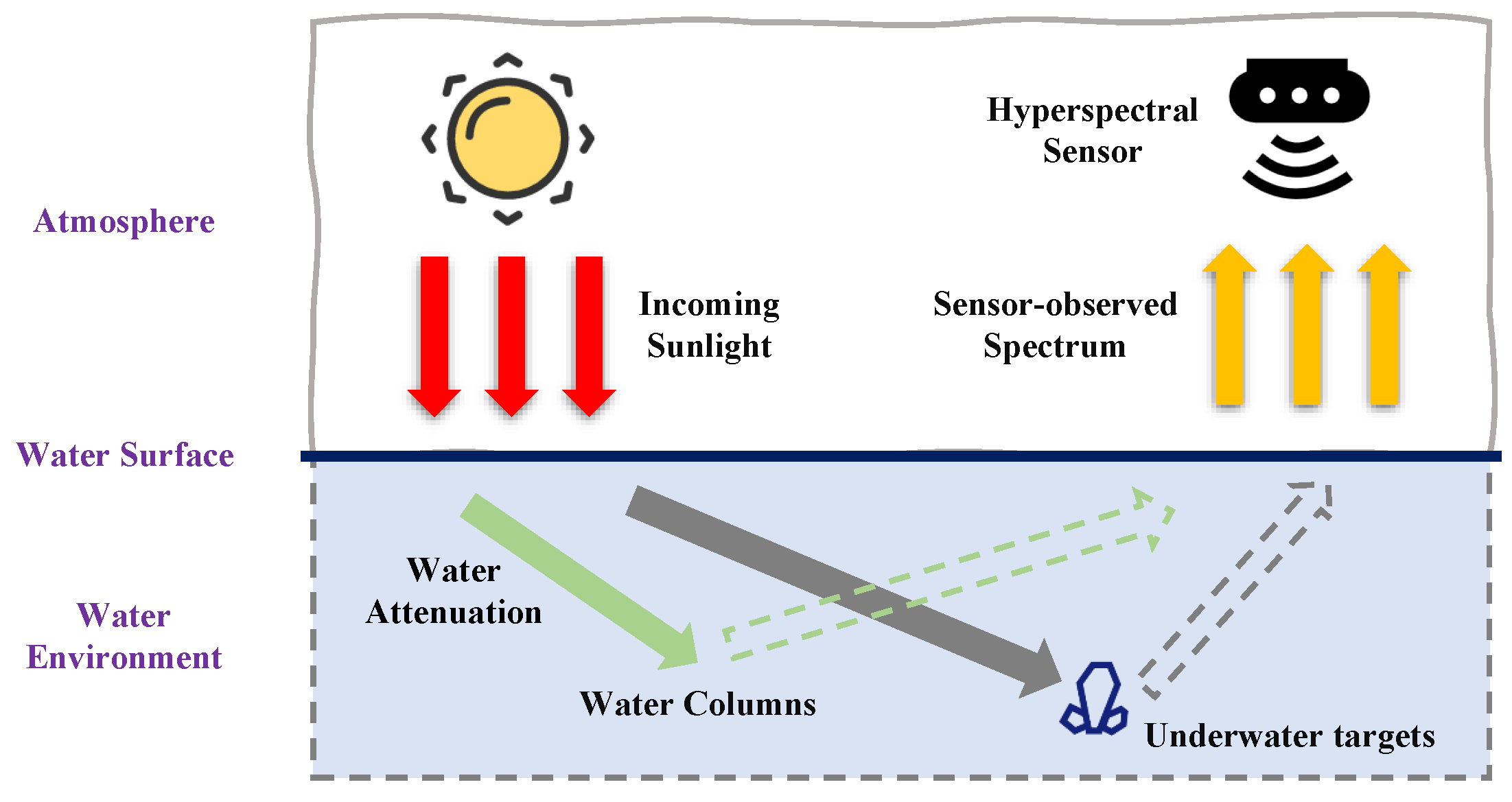
With the development of hyperspectral oceanography, classical bathymetric model [31] has been proposed based on the generation process of an hyperspectral image which is illustrated in Figure 1. In principle, this bathymetric model is established as a mathematical formula to describe the components of sensor-observed spectrum in an underwater HSI, which can be depicted as follows [31]:

$$\mathit{r}\left(\lambda \right)={\mathit{r}}_{\infty }\left(\lambda \right)\left(1-e^{-2k\left(\lambda \right)H}\right)+\frac{{\mathit{r}}_B\left(\lambda \right)}{\pi }{e}^{-2k\left(\lambda \right)H},$$

(1)

where ${\mathit{r}}_{\infty }\left(\lambda \right)$ and ${\mathit{r}}_B\left(\lambda \right)$ refer to spectrum of water column and land-based signature of desired target respectively. $k\left(\lambda \right)$ denotes the attenuation coefficients during light transmission process while H is the depth information.

From above equation, the sensor-observed spectrum $\mathit{r}\left(\lambda \right)$ is a linear combination of water column spectrum ${\mathit{r}}_{\infty }\left(\lambda \right)$ and target spectrum ${\mathit{r}}_B\left(\lambda \right)$, where the magnitudes of these two components are determined by the attenuation coefficients of water environment $k\left(\lambda \right)$ and the depth information of desired target H. Furthermore, the attenuation coefficients are the variables of wavelength which are assumed to be spatial-invariant in a small localized region.

As for the depth information, it is a vital parameter deciding the water column to be ‘optical shallow’ or ‘optical deep’ [32]. When it tends to be positive infinity, the sensor-observed spectrum comes to be the water column that acts as the background in the given underwater scene. Therefore, the value of depth information sometimes can be used as a criterion to distinguish the target spectra and background spectra.

2.2. Autoencoder

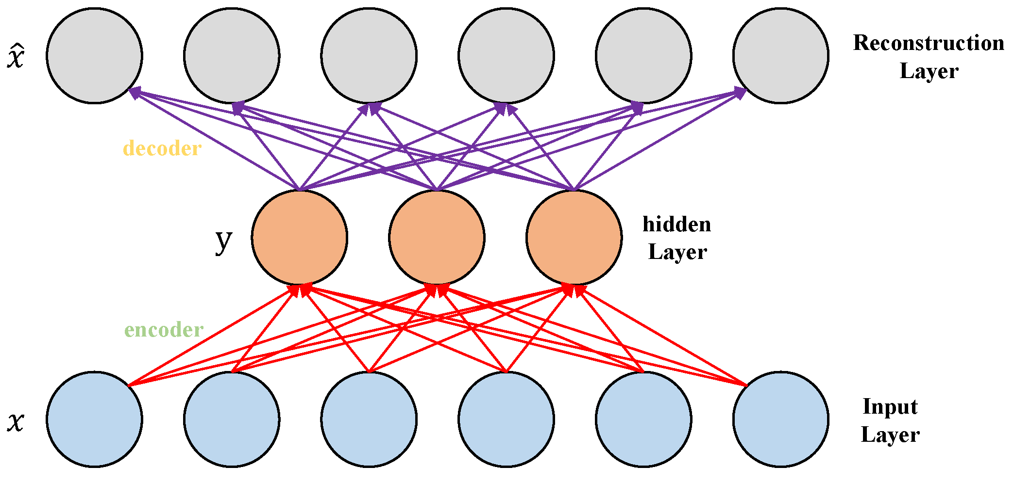
Generally speaking, a basic autoencoder network is composed of one visible layer with d inputs, one hidden layer with $h(d\gg h)$ units and one reconstruction layer with d outputs, which can be illustrated in Figure 2.

During the forward passing process, the input spectrum $x\in R^d$ is mapped to the hidden layer and then generate a specific spectral vector $y\in R^h$ named latent spectral vector. We generally call above procedure transforming the input vector into a low-dimension latent vector as the ‘encode’ step. After that, the latent vector is used to produce a vector $\widehat{x}\in R^d$ as the output of reconstruction layer that possesses the same size of input spectrum. This procedure, exploiting the low dimension latent vector to predict the output for reconstruction layer, usually denotes as ‘decode’ step.

The aim of training an autoencoder network is to determine the weight parameters combination that minimizes the reconstruction error between input spectrum x and reconstruction $\widehat{x}$. Once the autoencoder has been well-fitted, the decoder step can be exploited to transform input spectrum into a low-dimension vector and then different low-dimension vectors will establish a novel subspace. In this special subspace, the spectra vectors might possess some favorable characteristics contributing a great deal to HSI analysis.

3. Methodology

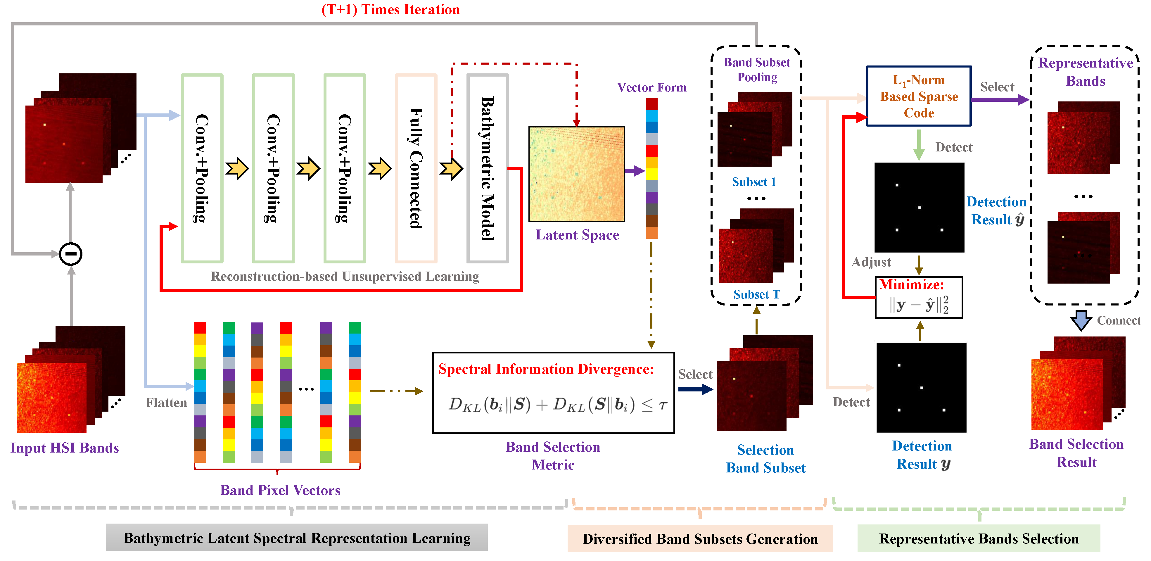
In this section, we will minutely demonstrate the details of our proposed method. The framework of BBS is illustrated in Figure 3 and its implementation process can be roughly summarized as three stages: bathymetric latent spectral representation learning, diversified band subset generation and representative band selection.

3.1. Bathymetric Latent Spectral Representation Learning

According to [33], the spectra of underwater target are indistinguishable from background due to the effect of water columns in underwater scenarios, leading to a decrease of detection performance. For the sake of alleviating this phenomenon, an intuitionistic perspective is to seek out the bands in which desired targets and background possess the best separability. Therefore, a criterion, contributing to select bands based on the measurement of separability between targets and background, is required to select out eligible bands.

As mentioned beforehand, a bathymetric model is a mathematical formula developed to depict the constituents of sensor-observed spectrum $r\left(\lambda \right)$ in underwater HSI. From Equation (1), we can find that depth information turns out to be a distinct feature to differentiate the background and target pixels. Since the depth information of background pixels is approximate to infinity, whereas it is only a bounded value for target pixels. Moreover, the attenuation coefficient $k\left(\lambda \right)$ is a variable of wavelength rather than spatial position. In other words, $k\left(\lambda \right)$ is spatial location-invariant and can be regarded as a uniform constant for both background and target pixels. Then, we can come up with a new variable $H_K\left(\mathit{x}\right)$:

$$\begin{array}{cc}\hfill H_K\left(\mathit{x}\right)& =K\left(\lambda \right)·H\left(\mathit{x}\right)\hfill \\ \hfill & =\left\{\begin{array}{cc}\infty ,\hfill & \mathrm{if}\mathit{x}\mathrm{is}\mathrm{background}\mathrm{pixel};\hfill \\ \mathrm{bounded}\mathrm{value},\hfill & \mathrm{if}\mathit{x}\mathrm{is}\mathrm{target}\mathrm{pixel}.\hfill \end{array}\right.\hfill \end{array}$$

(2)

where $K\left(\lambda \right)$ refers to the water attenuation coefficients and $H\left(\mathit{x}\right)$ denotes as the depth information of pixel $\mathit{x}$.

Clearly, this new variable can be exploited as an excellent metric to distinguish the target and background pixels. Consequently, the subspace $\mathit{S}$ consisting of $H_K$ with different spatial position information is deemed as a subspace that is appropriate for UTD task. Therefore, the BLSRL scheme is proposed to determine this special subspace with the assistance of bathymetric model.

With the view point proposed in [34], an autoencoder is specialized in generating the subspace in an unsupervised manner. However, for a basic autoencoder, the physical essence of corresponding subspace might not be explainable and controllable. Since a subspace associated with $H_K$ is required, BLSRL scheme would employ the bathymetric model as the decoder part to modify the structure of a basic autoencoder network.

For an input pixel $\mathit{Y}$, it works as the input of encoder part, which is a stack form of T convolution layers and one fully connection layer. This encoder part would compress input pixel vector into a constant, which can also be interrupted as making a prediction for $H_K$ according to pixel vector $\mathit{Y}$:

$${\mathit{Z}}^{\left(t\right)}=\left\{\begin{array}{cc}f\left({\mathit{w}}^{\left(t\right)}\ast \mathit{Y}+{\mathit{b}}^{\left(t\right)}\right),\hfill & t=1\hfill \\ f\left({\mathit{w}}^{\left(t\right)}\ast {\mathit{Z}}^{(t-1)}+{\mathit{b}}^{\left(t\right)}\right),\hfill & t\ge 2\hfill \end{array}\right.$$

(3)

$$H_K=g\left(\widehat{\mathit{w}}·{\mathit{Z}}^{\left(T\right)}+\widehat{\mathit{b}}\right)$$

(4)

where ${\mathit{Z}}^{\left(t\right)}$, ${\mathit{w}}^{\left(t\right)}$, and ${\mathit{b}}^{\left(t\right)}$ represent the output, weight vector, and bias vector of the t-th convolution layer. $\widehat{\mathit{w}}$ and $\widehat{\mathit{b}}$ refer to the weight vector and bias vector of fully connected layer. Note that, $r_{\infty }\left(\lambda \right)$ can be determined as the pixel-wised mean vector of input HSI while $r_B\left(\lambda \right)$ is also known as prior knowledge. Therefore, the reconstructed input vector $\widehat{\mathit{Y}}$ is available with this prediction value $H_K$ when the bathymetric model is utilized as the decoder part:

$$\widehat{\mathit{Y}}={\mathit{r}}_{\infty }\left(\lambda \right)\left(1-e^{-2H_K}\right)+\frac{{\mathit{r}}_B\left(\lambda \right)}{\pi }{e}^{-2H_K}.$$

(5)

Clearly, the desired subspace can be acquired if we minimize the difference between input pixel $\mathit{Y}$ and $\widehat{\mathit{Y}}$. To further fit the training data set, BLSRL uses a multi-criterion reconstruction error as the objective function:

$$\mathcal{L}=\parallel \widehat{\mathit{Y}}{-\mathit{Y}\parallel }_2+\frac{\lambda }{\pi }arccos\frac{\widehat{\mathit{Y}}·\mathit{Y}}{\parallel \widehat{\mathit{Y}}{\parallel }_2{\parallel \mathit{Y}\parallel }_2},$$

(6)

where $\lambda$ denotes the hyper-parameter to maintain the trade-off between different constraints, and $\left|\right|·{\left|\right|}_i$ represents $L_i$-norm of a vector. The former term of the above formula is the reconstruction error in numerical aspect while the latter one can be considered as the penalty for shape discrepancy. Finally, once the autoencoder has been well-trained, we can determine the desirable subspace $\mathit{S}$ with specified physical meanings from the output of the encoder part.

3.2. Diversified Band Subsets Generation

There is no doubt that the bands selected from input HSI should be similar to the obtained subspace $\mathit{S}$. That is to say, the space $\mathit{S}$ works as the reference map, and the spectral distance from $\mathit{S}$ refers to the band selection metric. It is noticeable that this spectral distance should be related to the pixel value distribution instead of pixel values because the similarity in distribution aspect is sufficient to guarantee the capacity of distinguishing target and background for the selected bands. Consequently, BBS employed the SID [35] between the i-th testing band ${\mathit{b}}_i$ and subspace $\mathit{S}$ as the band selection metric, while the selection rule can be formulated as follows:

$$\begin{array}{c}\hfill (\tilde{i})=\left\{\mathrm{SID}({\mathit{b}}_i,\mathit{S})\le \tau \right\},\end{array}$$

(7)

where $\tilde{i}$ represents the index of the selected band, and $\tau$ denotes the hyper-parameter to control the size of the calculated band subset.

With Equation (7), it is ready to acquire a favorable band selection result. However, this band selection result may be not of good diversity, and it is a waste of the abundant spectral information of input HSI if the unselected bands are simply discarded. To tackle this issue, an iteration-based method is also proposed for both promoting the diversity of band selection result and making full use of the unselected bands. This method employs BLSRL scheme to yield a novel subspace from the remainder bands once again and selects out another band subset with rule mentioned in Equation (7).

Moreover, this process would be repeated until reaching the stopping condition and eventually several band subsets are derived from the input HSI. Intuitively, the novel subspace reflects the characteristic of its associated band subset; thus, it is essential to make the latest generated subspace be different from the former ones, for the sake of decreasing the redundancy and promoting the distinctness among different band subsets.

That is to say, the number of selected band subsets T is dependent on the similarity between the novel produced band subset and the existing band subsets. This viewpoint is adopted to design the terminal condition for above iterative process, and the terminal condition of the n-th iteration ($n\ge 2$) can be demonstrated as follows:

$$\bigcap _{i=1}^{n-1}\{\mathrm{SID}({\mathit{S}}_i,{\mathit{S}}_n)⩾\mathrm{SID}({\mathit{S}}_i,{\overline{\mathit{b}}}_i)\},$$

(8)

where ${\mathit{S}}_i\left({\mathit{S}}_n\right)$ refers to the $i\left(n\right)$-th subspace, ${\overline{\mathit{b}}}_i$ represents the mean vector of the i-th selected band subset and ${\bigcap }_{i=1}^{n-1}$ means that the conditions for all the existing band subsets should be met simultaneously. As for the physical essence of this terminal condition, the first term in Equation (8) denotes the inter-class discrepancy between different band subsets, and the second one is the intra-class difference with one band subset.

3.3. Representative Bands Selection

Owing to the high spectral resolution of HSI, adjacent bands would possess almost the same spectral features, and then the generated band subset may also possess some redundant information. Furthermore, it would have no impact or slight impact on the detection result if we remove these redundant bands. Following this perspective, a detection performance-guided representative band selection method is proposed to circumvent the redundant band problem.

Assume that the i-th band subset ${\mathit{B}}_i\in {\mathbb{R}}^{L\times W\times p}$ contains p bands $\{{\mathit{b}}_{i1},{\mathit{b}}_{i2},\cdots ,{\mathit{b}}_{ip}\}$$({\mathit{b}}_{ij}\in {\mathbb{R}}^{L\times W})$ and the land-based target signature is $\mathit{d}=\{d_1,d_2,\cdots ,d_p\}$. Constrained Energy Minimization (CEM) [36], a classical land-based target detection method, can be shown in the vector form:

$$\mathit{M}=({\mathit{b}}_{i1},{\mathit{b}}_{i2},\cdots ,{\mathit{b}}_{ip})·{(w_1,w_2,\cdots ,w_p)}^T$$

(9)

where $\mathit{M}$ refers to the detection result of CEM detector. Moreover, let $\alpha =\{{\alpha }_1,{\alpha }_2,\cdots ,{\alpha }_p\}$ denotes the selection vector, the representative band selection operation can be represented in following mathematical form:

$${\widehat{\mathit{B}}}_i=({\mathit{b}}_{i1},{\mathit{b}}_{i2},\cdots ,{\mathit{b}}_{ip})·{({\alpha }_1,{\alpha }_2,\cdots ,{\alpha }_p)}^T$$

(10)

where

$${\alpha }_j=\left\{\begin{array}{cc}0,\hfill & \mathrm{if}{b}_{ij}\mathrm{is}\mathrm{unselected}\hfill \\ 1,\hfill & \mathrm{if}{b}_{ij}\mathrm{is}\mathrm{selected}\hfill \end{array}\right.$$

(11)

Then, the CEM result on representative bands refers to:

$$\widehat{\mathit{M}}=\left({\mathit{B}}_i\mathit{\alpha }\right)·\mathit{w}={\mathit{B}}_i·\left(\mathit{\alpha }\mathit{w}\right)={\mathit{B}}_i·\widehat{\mathit{w}}$$

(12)

where $\widehat{\mathit{w}}=\mathit{\alpha }·\mathit{w}$ denotes the sparse form of CEM operator, and the sparse degree ${\left|\right|\mathit{w}\left|\right|}_0$ is used to control the number of representative bands. To reduce the degeneration of detection performance due to removing redundant bands, it is required to minimize the discrepancy between $\mathit{M}$ and $\widehat{\mathit{M}}$. Consequently, $\widehat{\mathit{w}}$ can be determined by solving this optimization problem:

$$\parallel \mathit{M}-\widehat{\mathit{M}}{\parallel }_2^2={∥\mathit{M}-{\mathit{B}}_i·\widehat{\mathit{w}}∥}_2,\mathrm{s}.\mathrm{t}.{\parallel \widehat{\mathit{w}}\parallel }_0\le q$$

(13)

where q represents the sparse degree control factor. Since solving $L_0$ regularized optimization is an NP-hard problem, we employ $L_1$ regularization in practical application. With the obtained sparse CEM operator $\widehat{\mathit{w}}$, the representative bands are readily achievable by selecting out the bands whose sparse CEM operator coefficients are nonzero values. Finally, the band selection result is generated by concatenating the representative bands of all the band subsets. To make a conclusion, the whole process of the proposed method is exhibited in Algorithm 1.

Algorithm 1 The total process of the proposed method

Input: HSI $\mathit{X}$, band subset size control factor $\tau$ and sparse degree control factor q

Output: Band selection result for hyperspectral underwater target detection

1:  Establish an autoencoder with bathymetric model according to Equation (5).

2:  Train autoencoder $\mathit{A}$ with HSI $\mathit{X}$ to minimize Equation (6).

3:  Exploit the encoder part of $\mathit{A}$ to generate the bathymetric-based subspace ${\mathit{S}}_{\mathbf{1}}$.

4:  Transform the HSI $\mathit{X}$ into a hyperspectral bands set $\mathbf{B}$.

5:  $t\leftarrow 1$.

6:  while the terminal condition in Equation (8) is not satisfied do

7:         Produce the t-th band subset ${\mathbf{b}}_{\mathbf{t}}$ from $\mathbf{B}$ with subspace ${\mathit{S}}_{\mathit{t}}$ with Equation (7);

8:         Update the hyperspectral bands set $\mathbf{B}$ based on: $$\mathbf{B}\leftarrow \mathbf{B}-{\mathbf{b}}_{\mathbf{t}};$$

9:         $t\leftarrow t+1$

10:         Train autoencoder $\mathit{A}$ with hyperspectral bands set $\mathbf{B}$ to minimize Equation (6).

11:         Use the encoder part of $\mathit{A}$ to yield a new bathymetric-based subspace ${\mathit{S}}_{\mathit{t}}$ from hyperspectral bands set $\mathbf{B}$;

12:  end while

13:  for $i=1,2,\cdots ,t$ do

14:        Compute the sparse form of band subset $b_i$ according to Equation (13);

15:        Select out the bands whose sparse coefficients are nonzero values as representative bands for band subset $b_i$.

16:  end for

17:  Concatenate the representative bands of all the band subsets with the original band sequence to generate final band selection result.

4. Experiments

In this section, we performed plenty of experiments on different underwater datasets to demonstrate the effectiveness and efficiency of the proposed method. At the very beginning, the detailed information of experimental datasets will be briefly introduced. After that, we will state the employed evaluation criteria and parameter settings for all the experiments in next subsection. Then, corresponding ablation studies are designed to validate the effectiveness of the innovativeness proposed in Section 3. Finally, in the rest of this section, we exploit the underwater detection performances to reflect the performance of different band selection methods and specify their corresponding discussions and analyses.

4.1. Dataset Description

To achieve the most comprehensive evaluation of the proposed method, we should perform all the experiments on real datasets. However, since this research topic is novel, there exist few datasets containing underwater targets up to now. Therefore, we have to create two distinct HSI underwater datasets according to the scheme proposed by [32], which simulates the situations that desired targets locate in two different underwater scenes with disparate depth information. More specifically, in each underwater scenario, one specific material with four different depth information types are exploited as the desired underwater target placed in different spatial locations.

In other words, four different but relevant targets were contained in each dataset. As for the dataset generation scheme, we have summarized it into Algorithm 2. It is worth mentioning that the water attenuation coefficient $k\left(\lambda \right)$, which are required, as prior information should be determined beforehand. IOPE-Net [33] works as an excellent tool to address this issue. Furthermore, a real data collected by ourselves is also employed to demonstrate the performances of our method. Then, with the contribution of IOP-Net and Algorithm 2, we eventually achieve two synthetic data sets and one real data set:

Algorithm 2 The process of generating experimental datasets

Input: Real-world underwater HSI set $\mathbf{H}$, water attenuation coefficient $k\left(\lambda \right)$

Output: Underwater target detection data sets

1:  for real-world underwater HSI $\mathbf{h}\in \mathbf{H}$ do

2:        Acquire the water column spectrum $r_{\infty }\left(\lambda \right)$ by calculating the mean vector of real-world underwater HSI $\mathbf{h}$;

3:        Select the spectra of one specific material from USGS spectral library [37] as the desired target spectrum $r_B\left(\lambda \right)$;

4:       Produce the four distinct underwater target spectra $r\left(\lambda \right)$ with the water column spectrum $r_{\infty }\left(\lambda \right)$, desired target spectrum $r_B\left(\lambda \right)$ and four different depth information H according to Equation (1);

5:        Embed the generated target spectra into the real-world underwater HSI $\mathbf{h}$ at different spatial locations.

6:  end for

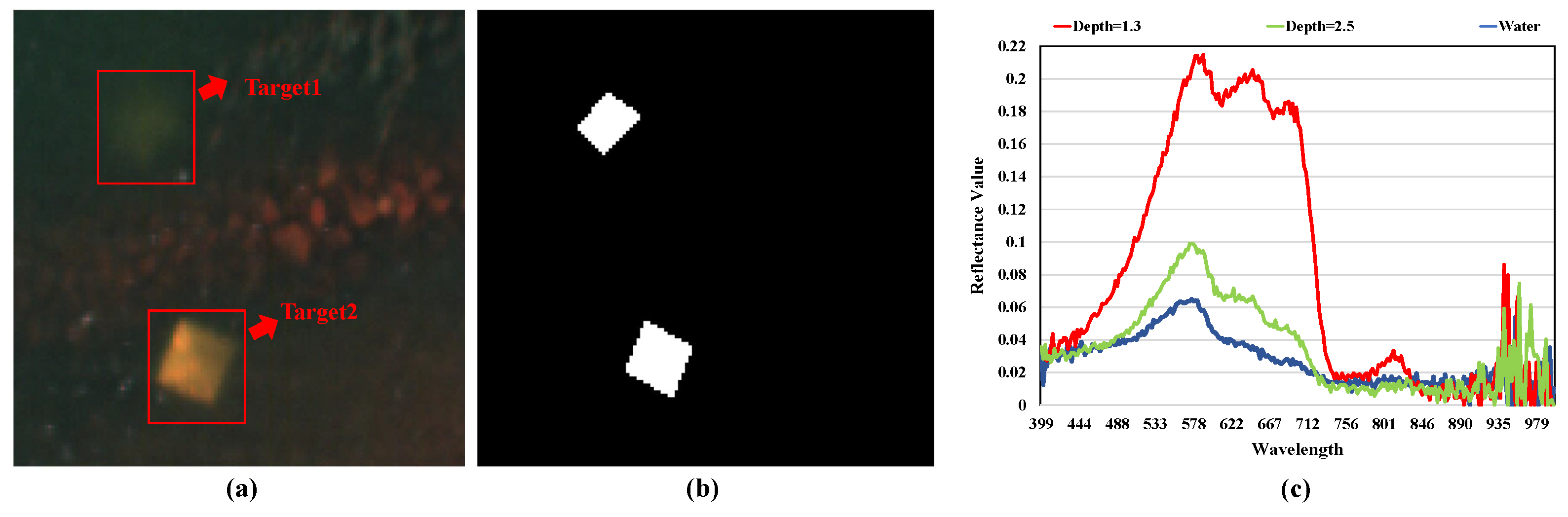
(1) Nano-Hyper Data Set: The real data is obtained by the Nano-Hyperspec sensor at Qianlu Lake Reservoir Changsha City, Hunan Province, China on 10 July 2021. The spectral solution of this data is 2.2 nm, and its wavelength ranges from 400 to 1000 nm. To conduct corresponding experiments, we segment out a chip with $137\times 137$ pixels that contains the desired underwater targets. In terms of the underwater targets, they are yellow metal plates whose sizes refer to 1 × 1 m. Considering the turbidity of lake water, we only set the targets at the shallow depths of 1 and 1.5 m. The detailed information of this real data set is exhibited in Figure 4.

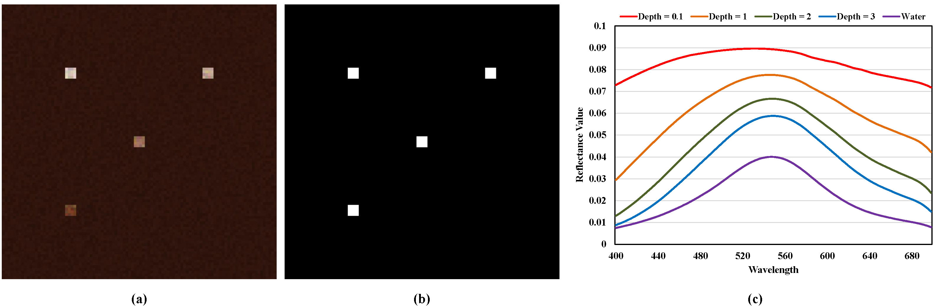
(2) Synthetic Data Based on Turbid Water HSI: The first synthetic dataset is derived from a turbid water HSI whose water inherent optical properties are recorded in [38]. This turbid water HSI is used to mirror the scene that desired targets locate in a muddy water environment. Its spatial resolution refers to $100\times 100$, and the spectral region of this HSI ranges from 400 to 700 nm with 150 bands. Furthermore, we denote the sheet metal material as targets of interest. Their corresponding depth information is 0.1, 1, 2, and 3 m, respectively. We illustrate the detailed information of this dataset in Figure 5.

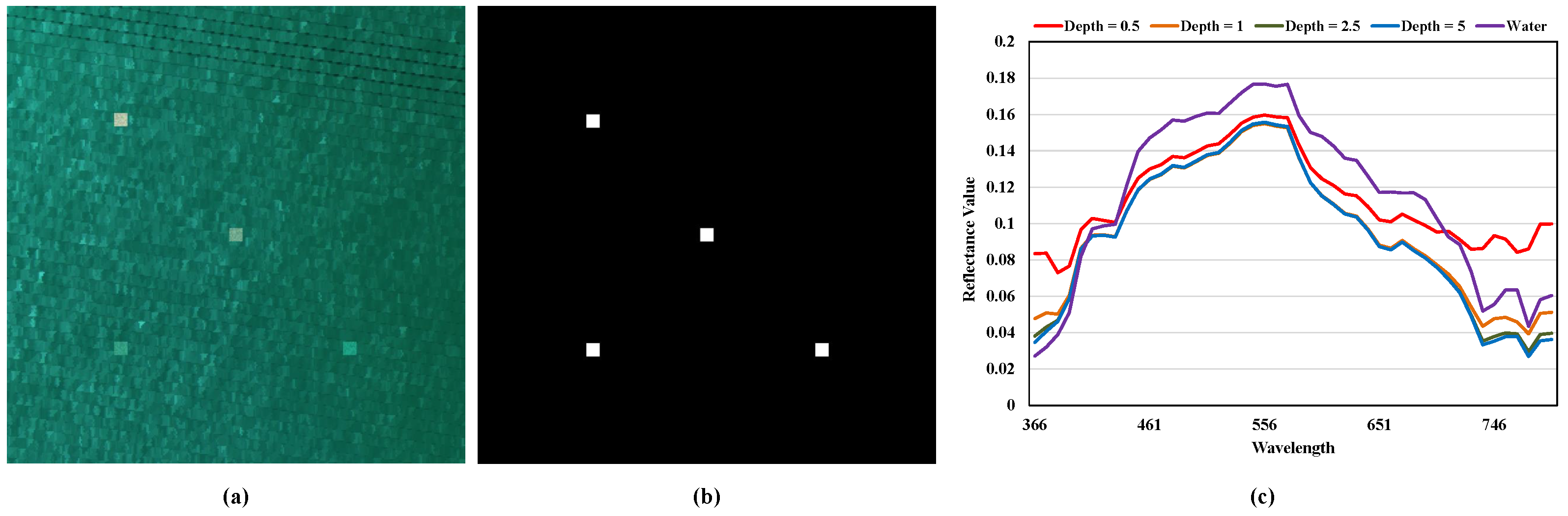
(3) Synthetic Data Based on Sea Water: The second synthetic dataset is established based on a hyperspectral sea water image, which is collected by Airborne Visible Infrared Imaging Spectrometer (AVIRIS) at a gullet locating in Galveston Bay, Texas. In general, the sea water is always more pellucid than other types of water. Consequently, this dataset can be regarded as a representation of clear water situation. This specific sea water image possesses 224 bands covering from 366 to 2495 nm at 9.5 nm spectral resolution. As for its spatial resolution, an image chip with $384\times 384$ pixels are segmented out as the experimental dataset. Moreover, the reflectance spectra of alunite material are chosen as the desired target spectra. We set the depth values of different underwater targets as 0.5, 1, 2.5, and 5 m. Similarly, Figure 6 is utilized to demonstrate the detailed information about the second dataset.

In summary, we list the key information of these two produced datasets in

Table 1. The summary of the important information for all the experimental datasets.

Dataset	Spatial Solution	Band Numbers	Target Material	Depth Information
Nano-Hyper	$137\times 137$	270	Metal plates	1 m and 1.5 m
Turbid water	$100\times 100$	150	Sheet metal material	0.1 m, 1 m, 2 m and 3 m
Sea water	$384\times 384$	224	Alunite material	0.5 m, 1 m, 2.5 m, and 5 m

. Meanwhile, these datasets are renamed as “Nano-Hyper”, “turbid water”, and “sea water” in the remainder of this paper.

4.2. Experimental Details

For the sake of introducing the experimental results in a more comprehensive manner, some necessary experimental details should be introduced in advance. There is no doubt that how to evaluate the performances of comparison methods is vital information for our experiments. Thus, we will briefly exhibit the evaluation criteria in the first part. After that, the experimental settings for different employed datasets are introduced in the rest of this section.

(1) Evaluation Criteria: Band selection methods work as a pre-processing operation for other HSI analysis application, whose performance cannot be measured directly. Since our proposed method is designed specifically for underwater target detection, the performances of detection results associated with different band selection methods can, thus, be exploited as the performance measurement.

To evaluate the performance of the detection results qualitatively, we use the receiver operating characteristic (ROC) curve as the first criterion. ROC, the most used metric in computer vision detection tasks, is devoted to depicting the relationship between the target detection probability $P_d$ and the false alarm rate (FAR) $P_f$ [39]. More specifically, the FAR $P_f$ denotes the percentage of falsely-detected pixels among all the testing pixels:

$$p_f=\frac{N_f}{N}$$

(14)

where $N_f$ refers to the quantity of falsely-detected pixels, and N is the amount of testing pixels contained in the input image. At the same time, the target detection probability $P_d$ reflects the ratio between correctly-detected pixels and the desired target pixels:

$$P_d=\frac{N_c}{N_t}$$

(15)

where $N_c$ is the number of correctly-detected pixels and $N_t$ represents the amount of desired target pixels. Note that, if the ROC curve of one method remains over other methods, it indicates that this method has achieved the best detection performance among all the comparison methods. In addition, the area under the ROC curve (AUC) values is another excellent metric to measure the performance of the detection results in a quantitative way.

(2) Dataset Pre-processing: Before employing the datasets to accomplish corresponding experiments, we should pre-process these datasets at the very beginning. Considering the effect of atmospheric interference, a classical atmospheric correction model ATCOR [40] is utilized to pre-process the input HSI data sets.

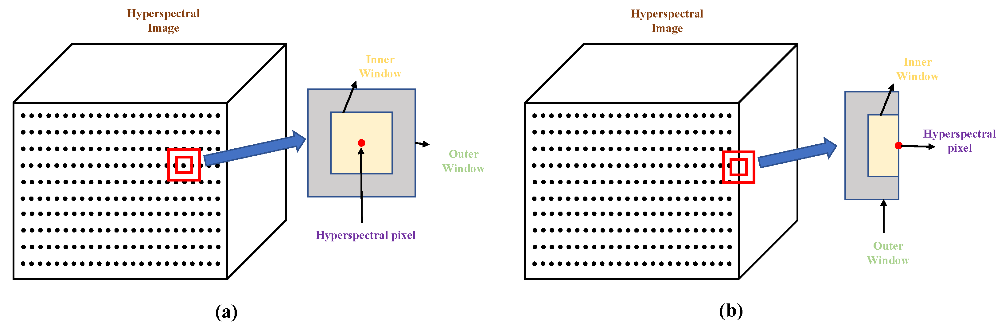
As for the water-surface effects, they will transform some pixels into sun glints, which act as the noisy points for the input hyperspectral imagery. For the sake of tackling this issue, we design a dual-window based local average strategy as a specific sun glints filter to pre-process input hyperspectral imagery. Since sun glints always pollute a pixel block instead of a single pixel, the inner window works as a guard window to ensure that average result will not be affected by the polluted pixels.

Then, owing to the local similarity, each pixel will be replaced by the average result of pixels located between the inner window and outer window. Exploiting the spatial resolution as a criterion, the sizes of inner window and outer window for the turbid water data set are 2 and 4. In terms of the sea water data set, the corresponding sizes are 3 and 7. The illustration of the proposed average strategy is demonstrated in Figure 7.

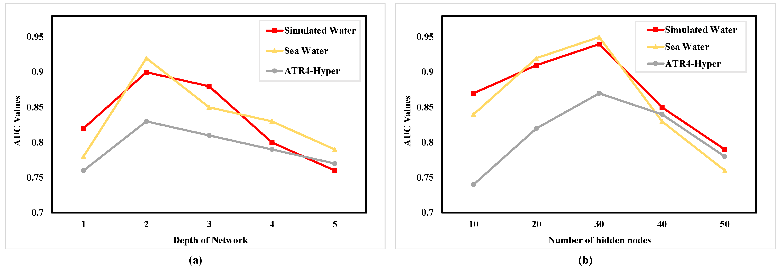
(3) Network parameter analysis: The autoencoder is the main part of bathymetric latent spectral representation learning in our proposed method. Thus, the depth of network and the amount of hidden nodes are vital parameters for the band selection method. The more network layers and hidden nodes, the stronger feature extraction ability the autoencoder embodies. However, more layers and nodes can also lead to more network parameters, long training time, and overfitting. To determine these two parameters, different values are set to find an optimal combination.

While finding the best depth of network, the number of hidden nodes is 50 (to make each hidden layer possess sufficiently strong feature extraction ability). Similarly, when analyzing the impact of the number of hidden nodes, the depth of network is set as result determined in last step. As demonstrated in Figure 8, we can find that if we set the depth of network as 2, our proposed method can achieve the best performance. Then, the depth of network is fixed as 2, and it can be observed that 30 is the best hidden node amount.

(4) Experimental settings: There exist three different kinds of experimental settings required to be stated: hyper-parameter setting, comparison methods, and experimental conditions.

In this paper, we raise three different hyper-parameters: regularization coefficient $\lambda$, band subset size control factor $\tau$, and the sparse degree control factor q. The first hyper-parameter has less impact on the other hyper-parameters, and then we can tune this hyper-parameter individually. Since $\lambda$ replaces the weight of spectral angle loss in objective function, we will find the optimal value range from 0.01 to 0.1 with a fixed step of 0.01. The concrete values of this parameter for different selected band amounts in all the datasets are listed in

Table 2. The hyper-parameter settings and their corresponding selected band amounts for different datasets.

Dataset	Hyper-Parameter $\mathit{\lambda }$	Hyper-Parameter $\mathit{\tau }$	Hyper-Parameter q	Selected Band Amount
Nano-Hyper	0.005	0.1	0.1	22
	0.01	0.2	0.2	34
	0.02	0.3	0.3	58
Turbid water	0.02	0.1	0.1	8
	0.03	0.2	0.2	18
	0.05	0.3	0.3	27
Sea water	0.01	0.1	0.1	17
	0.02	0.2	0.2	27
	0.04	0.3	0.3	42

.

In terms of band subset size control factor $\tau$ and sparse degree control factor q, these are the critical hyper-parameters to determine the amount of selected bands. Band subset size control factor $\tau$ affects the process of diversified band subset generation, while sparse degree control factor q is proposed for representative band selection. Since representative band selection operation is conducted on generated diversified band subsets, we should determine the value of $\tau$ at the very beginning.

If the band selection amount is not determined and we would like to find optimal number of bands, the parameter adjustment strategy is demonstrated as follows. To alleviate the effect of sparse degree control factor q, its value is set to 1, which makes all the bands in one cluster representative bands. Then, we find the best $\tau$ based on the underwater target detection performance. After that, $\tau$ is fixed as prior knowledge, and we find the optimal q that helps to achieve first-rank band selection performance. With the fixed $\tau$ and q, we can eventually determinate the optimal number of bands.

When the number of bands has been determined beforehand, we can exploit the binary search strategy to determine the combination of these two parameters that achieves the best band selection performance and meets the the number of selected bands. The concrete values of these two hyper-parameters and their corresponding selected band amounts for different datasets are listed in Table 2.

To further demonstrate the band selection performances, we employ three representative band selection methods OCF [41], ONR [42], and LBS [43] as the comparison methods. Furthermore, we also employ a specific band selection named best contrast and lowest attenuation (BCLA) method as another comparison method. This method finds wavelengths where the contrast between the target and the background (the sea floor) is the highest and the attenuation constant is the lowest.

Finally, as for the experimental hardware conditions, all the algorithms are performed with an Intel(R) Core (TM) i9-10920X CPU machine and 64 GB of RAM. The corresponding operation system refers to Windows 10 operating system, while the deep learning framework Pytorch 1.7.0 is used to accomplish all the codes.

4.3. Ablation Study

In this subsection, we will perform some special experiments for ablation studies to demonstrate the validity of the innovation points proposed in our research work.

(1) Effectiveness Evaluation of the iteration-based band subset generation scheme (IBSGS): In Section 3.2, we proposed a novel band subset generation scheme named IBSGS. This scheme is employed to make full use of the hyperspectral information while promoting the diversity of band selection results. Therefore, for the sake of confirming the effectiveness of this specific scheme, we conduct the BBS without it as the comparison. We selected 10, 20, and 30 bands from employed dataset to demonstrate the effect of IBSGS under different selected band amount conditions. The corresponding results are listed in

Table 3. The AUC values of the UTD results for confirming the effectiveness of IBSGS.

Number of Selected Bands	Nano-Hyper		Turbid Water		Sea Water
	BBS (N)	BBS (Y)	BBS (N)	BBS (Y)	BBS (N)	BBS (Y)
10	0.68	0.73	0.81	0.85	0.91	0.93
20	0.74	0.79	0.84	0.91	0.92	0.96
30	0.76	0.83	0.86	0.95	0.94	0.98
Average	0.727	0.783	0.834	0.903	0.923	0.957

The bold entries represent the best performance in each row.

, where the characters (Y and N) in parentheses imply whether BBS contains IBSGS.

From this table, we can draw the conclusion that IBSGS will contribute greatly to the UTD results, which also reflects its profitable effect on the promotion of diversity of the band selection results. In addition, the contribution of IBSGS turns out to be proportional to the numbers of selected bands. In other words, the benefit of IBSGS will improve as the amount of selected bands increases. Considering the computation burden, there is a trade-off between the effect of IBSGS and the amount of selected bands. In practical application, it is recommended to exploit IBSGS when the number of selected bands refers to a relativlye large value.

(2) Effectiveness Evaluation of the sparse representation-based representative band selection strategy (SRRBSS): Considering the interference of redundant information between adjacent bands, we have come up with a sparse representation-based strategy to pick out the representative bands for all the generated band subsets, named SRRBSS. To verify the practicability of SRRBSS, the intra-class variability of a band subset is utilized as the metric since SRRBSS is used to alleviate the correlation among adjacency bands. To determine a quantitative result, statistical magnitude $\sigma$ is calculated, which can be formulated as follows:

$$\sigma =\sum _{i=1}^n∥{\mathit{x}}_i-\overline{\mathit{x}}∥$$

(16)

where ${\mathit{x}}_i$ and $\overline{\mathit{x}}$ represent the i-th band and the mean vector of the band selection result, respectively. n denotes the number of selected bands. For statistical magnitude $\sigma$, a larger value of this parameter is achievable when the bands contained in one subset are more different from their average band, which indicates that this band subset has less redundancy information. Analogously, we perform the BBS without SRRBSS, as the reference and the comparison results are shown in

Table 4. The values of statistical magnitude $\sigma$ for confirming the effectiveness of SRRBSS.

Number of Selected Bands	Nano-Hyper		Turbid Water		Sea Water
	BBS (N)	BBS (Y)	BBS (N)	BBS (Y)	BBS (N)	BBS (Y)
10	0.14	0.41	0.17	0.54	0.08	0.33
20	0.25	0.63	0.31	0.62	0.27	0.57
30	0.43	0.71	0.46	0.77	0.41	0.62
Average	0.273	0.583	0.313	0.643	0.253	0.507

The bold entries represent the best performance in each row.

.

According to the comparison results, the bands selected by the BBS method with SRRBSS possess a better intra-class irrelevance. To further explore the effect of irrelevance on UTD tasks, the corresponding detection performances are evaluated and demonstrated in

Table 5. The AUC values of the UTD results for confirming the effectiveness of SRRBSS.

Number of Selected Bands	Nano-Hyper		Turbid Water		Sea Water
	BBS (N)	BBS (Y)	BBS (N)	BBS (Y)	BBS (N)	BBS (Y)
10	0.59	0.73	0.69	0.85	0.71	0.93
20	0.62	0.79	0.73	0.91	0.78	0.96
30	0.71	0.83	0.77	0.95	0.84	0.98
Average	0.64	0.783	0.73	0.903	0.776	0.957

The bold entries represent the best performance in each row.

. Unsurprisingly, SRRBSS can boost the performances of UTD tasks, while the performance gaps are pretty severe. This phenomenon shows the necessity of employing SRRBSS to achieve a favorable band selection result.

4.4. Band Selection Performances and Discussion

In this subsection, we will minutely demonstrate the band selection results and their associated discussions. As mentioned beforehand, the underwater target detection performances are exploited as the band selection performance measures since our method is proposed particularly for underwater target detection task. Therefore, the CEM method is utilized as the underwater target detector in our experiments. To further demonstrate the band selection performances, we employ four representative band selection methods OCF [41], ONR [42], LBS [43], and BCLA as the comparison methods.

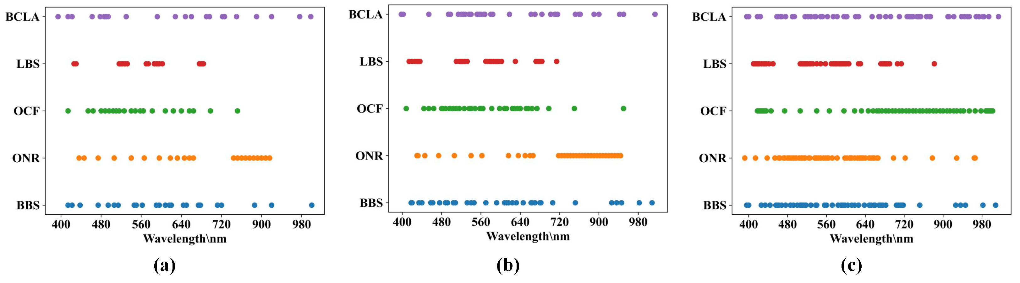
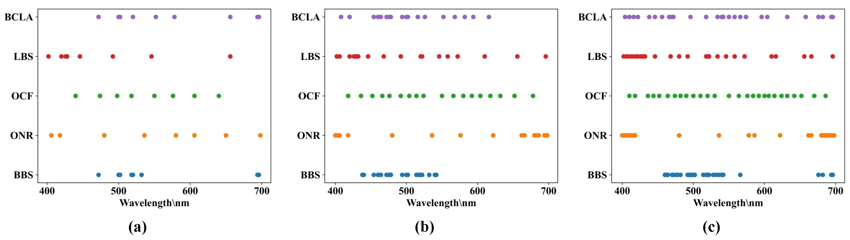
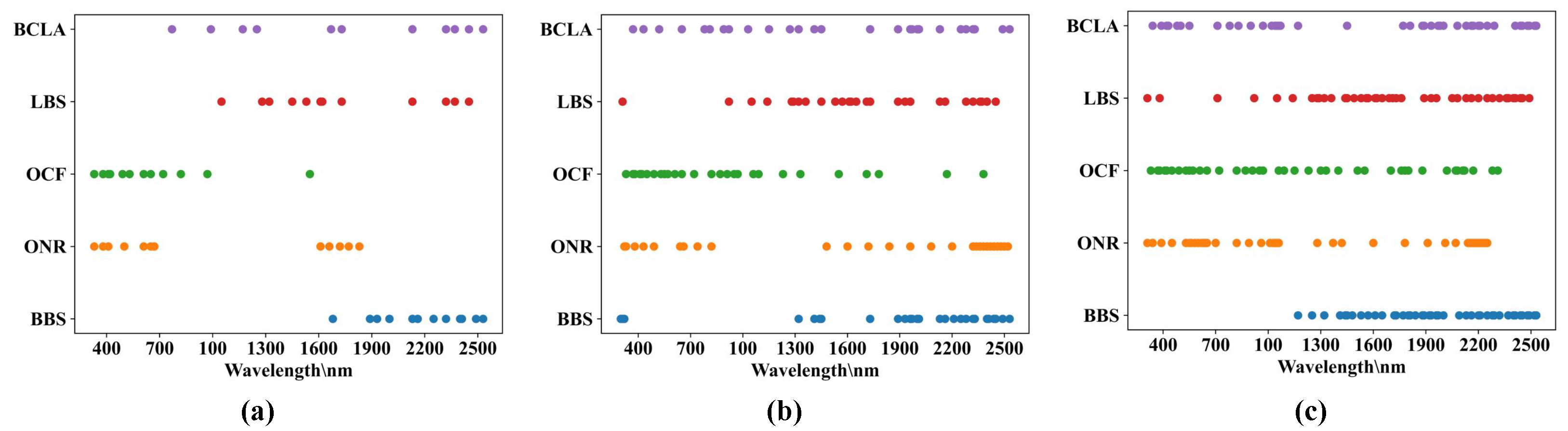
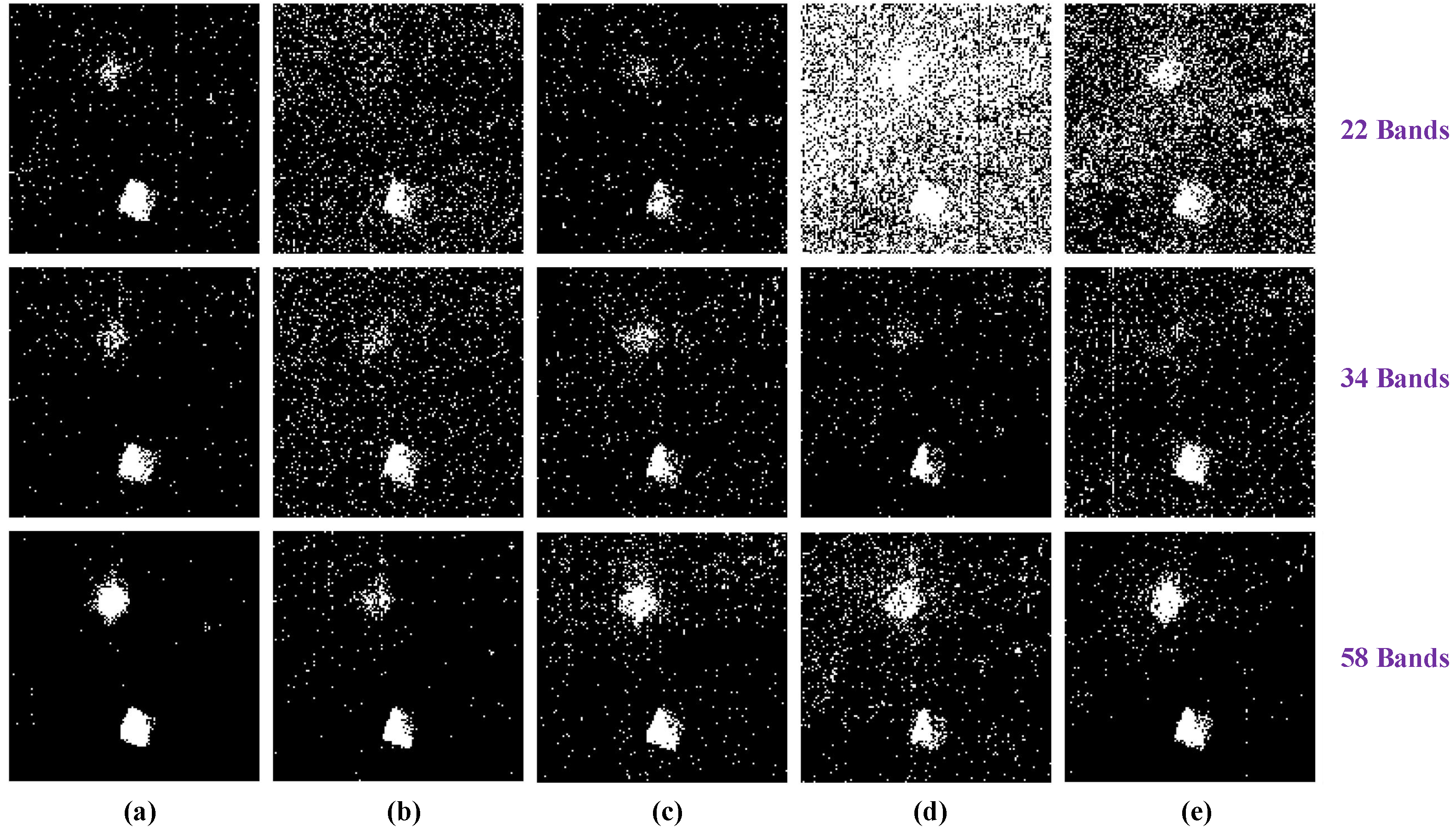
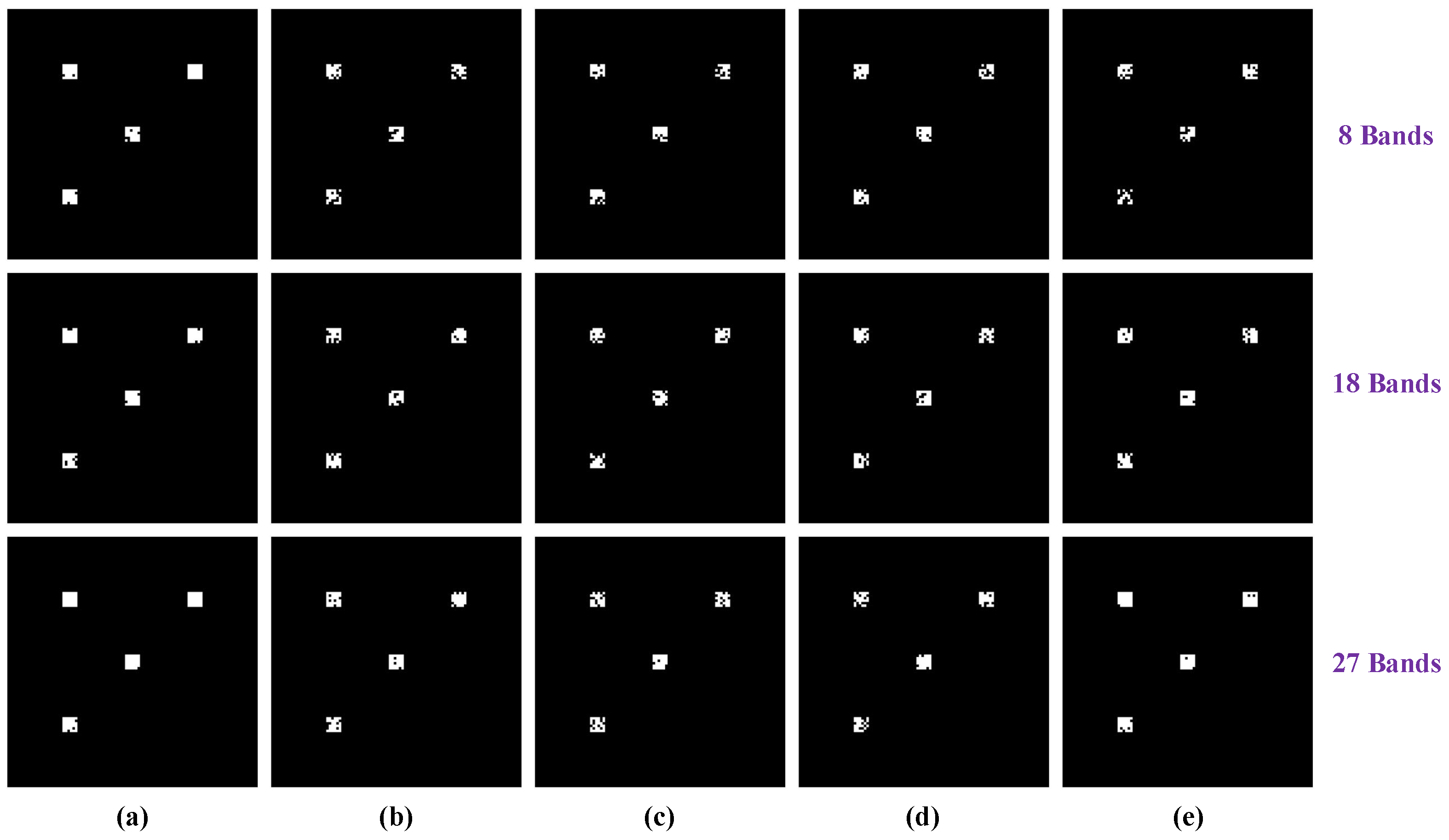
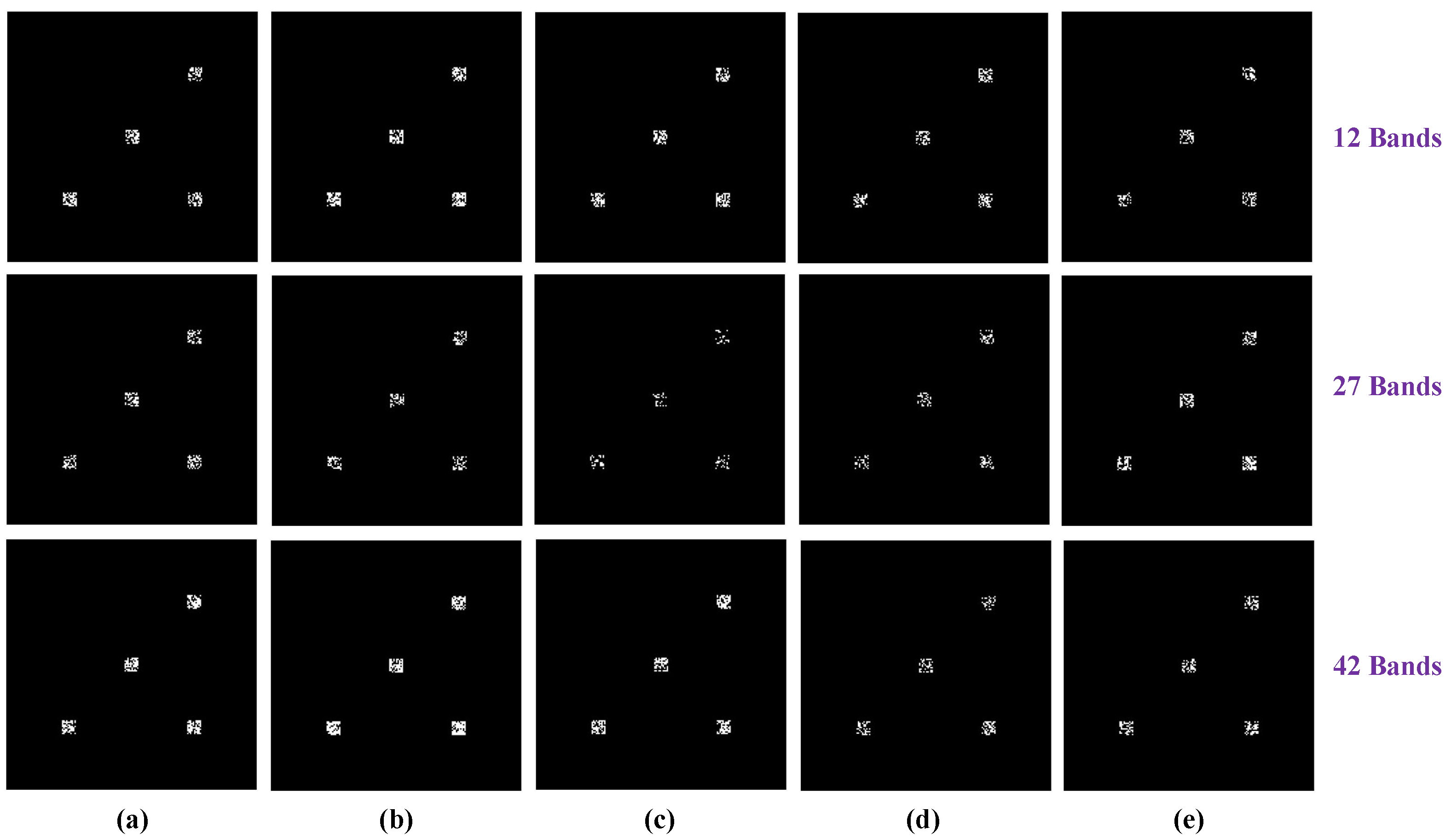
At the very beginning, we visualize the band selection results in Figure 9, Figure 10 and Figure 11. In these figures, all the x axes represent the wavelengths of selected bands, and then we can achieve the distribution of selected bands for different methods. Then, the underwater target detection performances are demonstrated from the visual aspect. Figure 12, Figure 13 and Figure 14 illustrate the reference maps (such as ground truths and detection maps) for all the UTD results.

According to the above visualized detection results, it is effortless to determine that the BBS-associated UTD results achieve the slightest difference with the ground truths based on the visual judgment. More importantly, the proposed method may contribute greatly to detecting the targets located in a deeper position. For instance, in the turbid water dataset, the CEM detector can integrally determine the targets located in the depth of 3 m from the band selection results derived from our method, while other band selection results may lead to a higher false negative rate.

As the numbers of selected bands increase, the UTD performances will be promoted for all the compared methods. However, this influence has less impact on our proposed method, which manifests that BBS can contribute greatly to the underwater detection task with less selected bands, and the bands selected by BBS are more representative and more appropriate for detecting underwater targets.

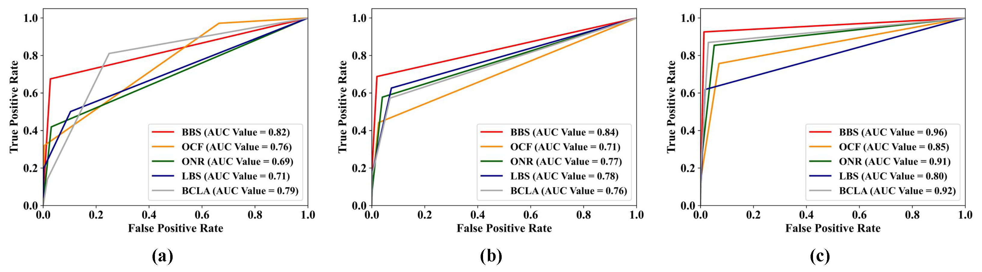
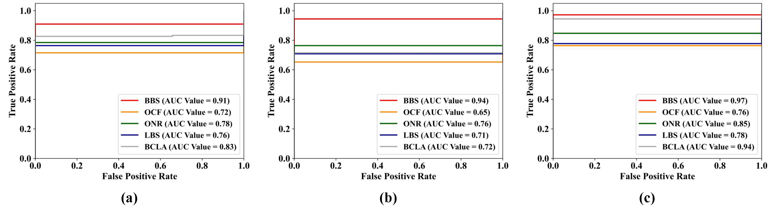
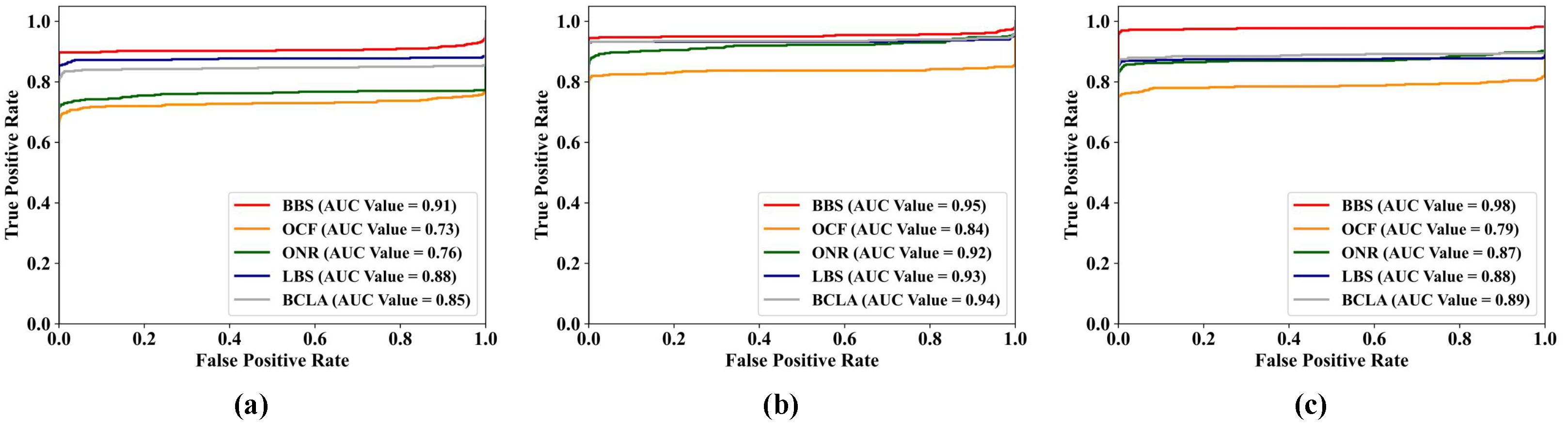
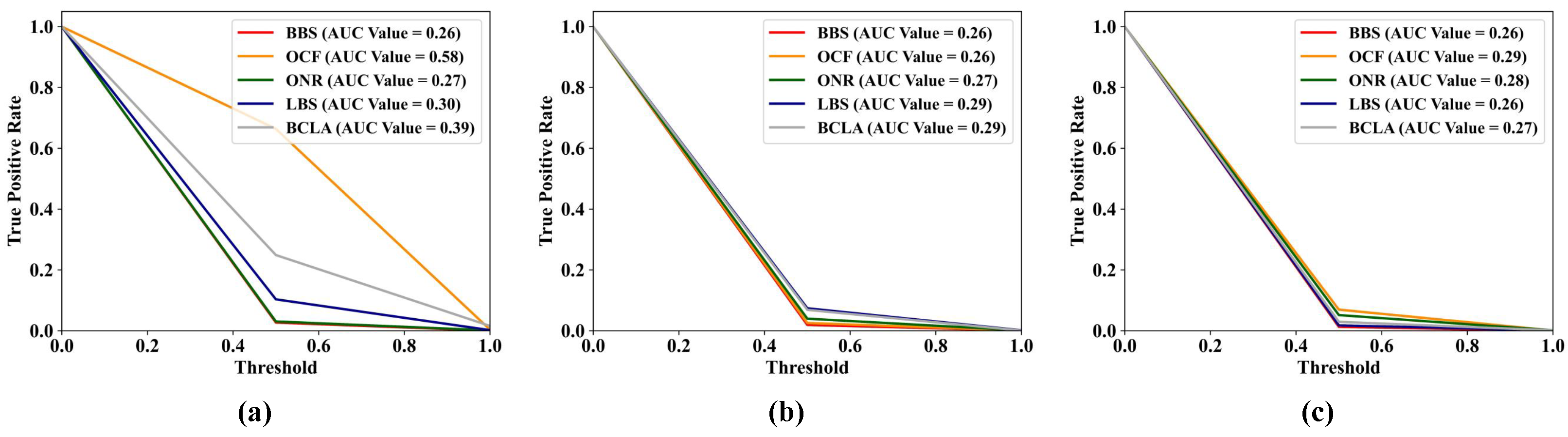
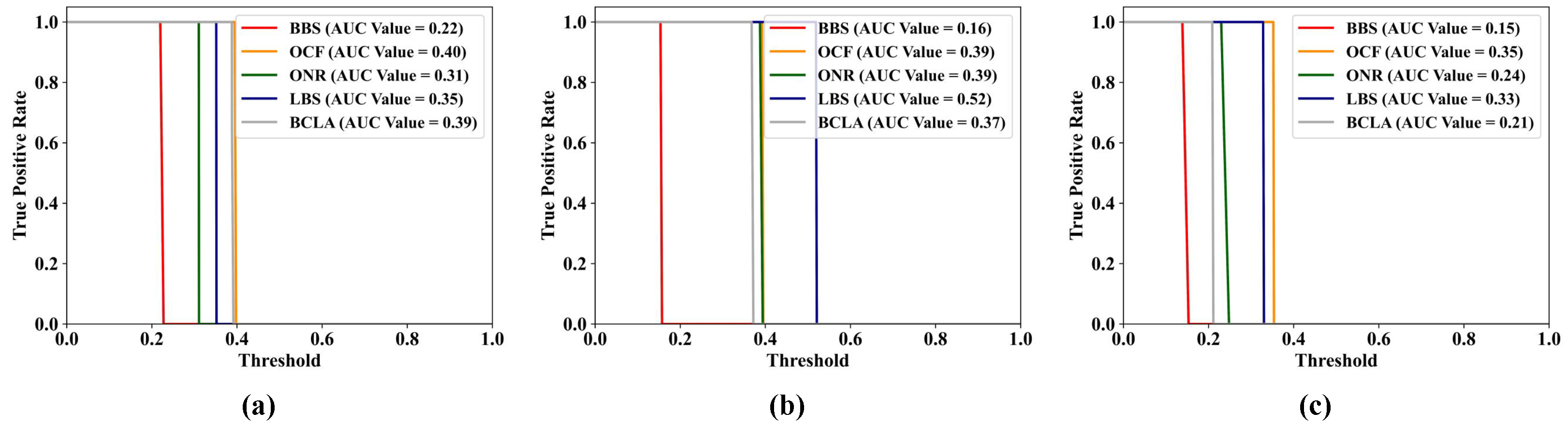
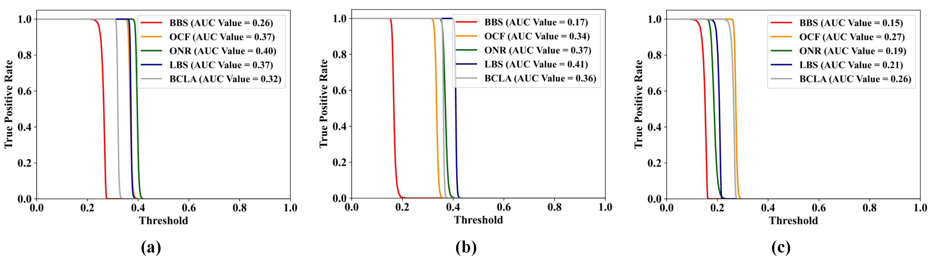
In order to conduct the qualitative analysis of the detection performance, the ROC curves of $(P_D,P_F)$ and $(P_F,Threshold)$ about the detection results were plotted as another detection performance measurement. Figure 15, Figure 16 and Figure 17 are associated with the ROC curves of $(P_D,P_F)$ with different selected band numbers for all the datasets. According to these two figures, all the ROC curves associated with proposed method remain over other curves in all the testing datasets with different selected band numbers. In addition, the Figure 18, Figure 19 and Figure 20 is used to depict the ROC curves of $(P_F,Threshold)$ for the underwater detection results.

To be specific, the curves relevant to BBS locate at the bottom of other compared methods under all the experimental conditions, which illustrates that BBS exposes a positive effect on reducing FARs for underwater target detection performances. With the aforementioned evidence, we can finally draw the conclusion that BBS can promote the underwater target performances in the aspect of detection accuracy and FAR.

Then, for the sake of achieving a quantitative comparison, the AUC values of ROC curves demonstrated from Figure 16, Figure 17, Figure 18, Figure 19 and Figure 20 were calculated and are listed in the

Table 6. The AUC of $(P_D,P_F)$ for the UTD results on all the data sets with different band selection methods.

Number of Selected Bands	AUC Values for Nano-Hyper Data Set
	LBS	OCF	ONR	BCLA	BBS
22	0.71	0.76	0.69	0.79	0.82
34	0.78	0.71	0.77	0.76	0.84
58	0.80	0.85	0.91	0.92	0.96
Average	0.76	0.77	0.79	0.82	0.87
Number of Selected Bands	AUC Values for Turbid Water Data Set
	LBS	OCF	ONR	BCLA	BBS
8	0.76	0.72	0.78	0.83	0.91
18	0.71	0.65	0.76	0.72	0.94
27	0.78	0.76	0.85	0.94	0.97
Average	0.75	0.71	0.80	0.83	0.94
Number of Selected Bands	AUC Values for Sea Water Data Set
	LBS	OCF	ONR	BCLA	BBS
17	0.88	0.73	0.76	0.85	0.91
27	0.93	0.84	0.92	0.94	0.95
42	0.88	0.79	0.87	0.89	0.98
Average	0.90	0.79	0.85	0.89	0.95

The bold entries represent the best performance in each row.

and

Table 7. The AUC of $(P_F,Threshold)$ for the UTD results on all the data sets with different band selection methods.

Number of Selected Bands	AUC Values for Nano-Hyper Data Set
	LBS	OCF	ONR	BCLA	BBS
22	0.35	0.40	0.31	0.39	0.22
34	0.52	0.39	0.39	0.37	0.16
58	0.33	0.35	0.24	0.21	0.15
Average	0.40	0.38	0.31	0.32	0.18
Number of Selected Bands	AUC Values for Turbid Water Data Set
	LBS	OCF	ONR	BCLA	BBS
8	0.39	0.58	0.27	0.30	0.26
18	0.29	0.26	0.27	0.29	0.26
27	0.26	0.29	0.28	0.27	0.26
Average	0.31	0.38	0.27	0.29	0.26
Number of Selected Bands	AUC Values for Sea Water Data Set
	LBS	OCF	ONR	BCLA	BBS
17	0.37	0.37	0.40	0.32	0.26
27	0.41	0.34	0.37	0.36	0.17
42	0.21	0.27	0.19	0.26	0.15
Average	0.33	0.33	0.32	0.31	0.19

The bold entries represent the best performance in each row.

. On the basis of Table 6, the detection performances combined with our proposed method have the largest AUC values, and all exceed 0.8. Furthermore, the average values of BBS are 0.87, 0.94, and 0.947 for the Nano-Hyper, turbid water data set, and sea water data set while the suboptimum method can only achieve 0.82, 0.797, and 0.85.

The statistical information contained in Table 6 confirms the superiority of improving detection accuracy in numerical aspect. In terms of the AUC values for the ROC curves of $(P_F,Threshold)$, the detection results derived from BBS achieved the lowest AUC values for all the datasets under different selected band amounts, which demonstrates that these detection results possess the best performances in FARs. That is to say, BBS succeeds in finding out the space where targets and backgrounds have the best separability, leading to effectively eliminating the interference of water background.

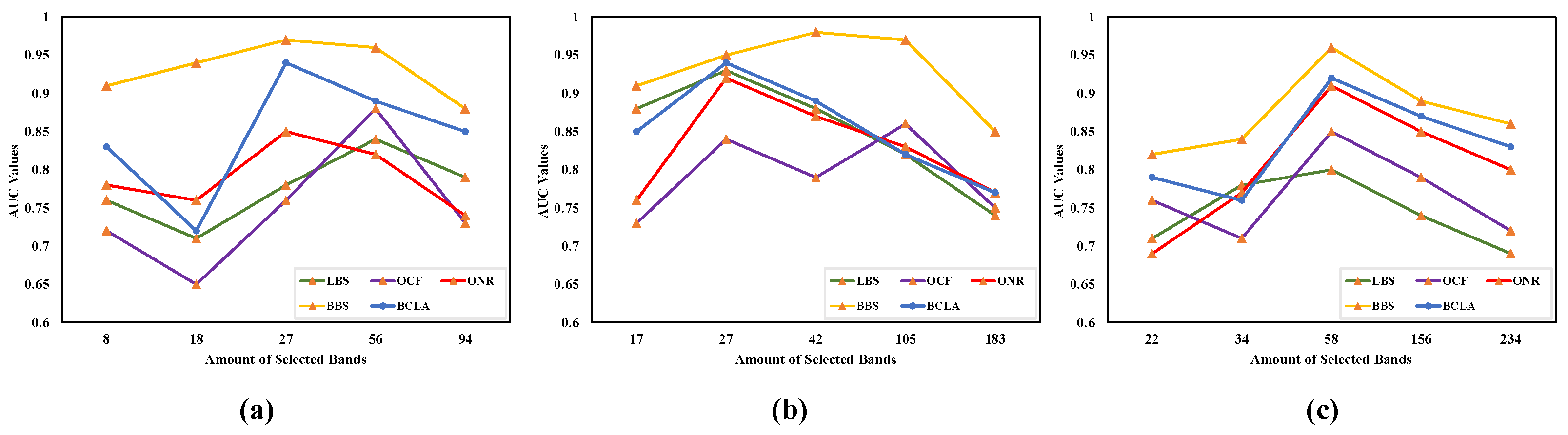
According to the above analyses, it is easy to find the selected band amounts would have great impacts on the final underwater detection result. Therefore, we change the values of subset size control factor $\tau$ and sparse degree control factor q to generate band selection results with different band amounts. To make a comprehensive comparison, the employed methods are also used to produce the band selection results with the identical band amounts. The relationship between underwater detection performance (AUC values of $(P_D,P_F)$) and band amounts is illustrated in Figure 21.

Based on this figure, for our proposed method, increasing the amount of selected bands will improve the performance of detection result at the very beginning. However, when the amount of selected bands exceeds a certain value, the detection performance will decrease as more bands were picked out. This phenomenon is satisfied with the ‘Hughes phenomenon’, and this indicates that, for the BBS method, we should determine its optimal selected band amount before using it.

Finally, the execution time of all the compared methods are determined to exhibit an efficiency comparison and the relevant results are presented in

Table 8. Average execution time (in seconds) of the compared methods for all the datasets.

Dataset	Execution Time (in Seconds)
	BBS	LBS	ONR	OCF	BCLA
Nano-Hyper	36.7081	3.8713	11.7812	19.6337	29.4203
Turbid water	27.7148	2.8456	8.7495	15.1754	23.7893
Sea water	42.4982	5.3969	14.8247	22.7496	37.4817
Average	35.6404	4.0199	11.7851	19.1862	30.2304

The bold entries represent the best performance in each row.

. We performed all the methods with experimental environment mentioned in Section 4.2. To yield a more fair comparison result, the final execution time is derived by averaging the execution time under different selected amounts. According to Table 8, LBS method achieved the best performances on both the average execution time and the execution time for each testing dataset.

Unfortunately, the time burden of BBS is the heaviest one among all the comparison methods. The reason accounting for this phenomenon is that BBS exploits an iteration-based scheme to pick out more band subsets for the sake of promoting the diversity of detection results and making full use of the spectral information. Therefore, the efficiency has been sacrificed to improve the effectiveness of our proposed method. However, it is worth mentioning that the time consumption of BBS is not too large, and it is tolerable in real-world applications.

In summary, we have confidence to make the conclusion that BBS is an effective band selection method to improve the detection performances of underwater target tasks.

4.5. The Limitation of Our Study

In this paper, we proposed a novel band selection method for underwater target detection tasks. Adequate experimental results confirmed the performance of our proposed method. However, there remain some limitations that must be dealt with in future research:

1.

The proposed method can only be applied in deep-water scenarios. The employed physical model (underwater bathymetric model in Equation (1)) in this paper is based on the assumption that the hyperspectral sensor will capture the reflectance deprived by the sea bottom. Thus, our proposed method does not consider the effects of the sea bottom and is proposed for deep-underwater scenarios. Consequently, the practical application scenario of our proposed method is limited, and we will attempt to modify the physical model to improve the generalization of our proposed method in future research.

2.

The proposed method leads to more burden on time and memory. Based on Table 8, we can find that the time burden of BBS refers to the heaviest one among all the comparison methods, since an iteration-based strategy is designed to promote the performance of the band selection results. Deep learning methodology is also exploited in our research work, and the method requires more computational memory and resource.

3.

The proposed method refers to a two-stage band selection method. The process of our proposed method can be divided into two stages: diversified band subset generation and representative band selection. There is no doubt that the performance of diversified band subset generation will affect the the performance of representative band selection, which might eventually undermine the final band selection results.

5. Conclusions

In this paper, we proposed an unsupervised band selection method called BBS for UTD tasks. This novel BBS consists of three indispensable parts: a bathymetric latent spectral representative learning scheme, iteration-based band subset generation strategy, and sparse representation-based representative band selection method. Considering the dependence between the target pixels and background pixels, BBS first exploits the bathymetric model to modify a basic autoencoder to determine a physically meaningful subspace.

In this special space, targets and background maintain the maximum distance, which is favorable to underwater target detection tasks. Therefore, the generated subspace is exploited as the reference to select out desired bands. Then, we developed an iteration-based strategy to divide the input HSI into massive subsets. The iteration-based strategy was designed to improve the diversity of the band selection results and the use ratio of hyperspectral information.

The corresponding experimental results mentioned in Section 3.2 confirmed the validation of this specific strategy. After that, a sparse representation-based approach was proposed to determine the representative bands for all the band subsets, which aims at reducing the redundancy in each band subset.

Similarly, some special tests were performed to demonstrate the usage of this sparse representation based approach. Finally, the band selection result was achieved by connecting the obtained representative bands in the original band sequence. The experiments on two synthesis data sets and one real data set demonstrated the performance of BBS. Comprehensive analysis in both qualitative and quantitative aspects also validates the effectiveness of our proposed method.

In summary, the major findings of this research work can be listed as follows:

• ${\mathit{H}}_{\mathit{K}}\left(\mathit{x}\right)$, the product of depth information and water attenuation coefficient, comes to be an excellent metric for designing band selection criterion. First of all, target pixels and background pixels possess different $H_K\left(\mathit{x}\right)$ values, then $H_K\left(\mathit{x}\right)$ can be regarded as a preeminent feature to differentiate these two kinds of pixels. Furthermore, compared with the depth information and water attenuation coefficient, our research found that it was easy to determine $H_K\left(\mathit{x}\right)$ in an unsupervised manner. In other words, $H_K\left(\mathit{x}\right)$ performed well in real-world applications.
• Making full use of the unselected bands contributes greatly to the diversify and the performance of band selection result. Most of the existing band selection methods merely select the bands from input HSI at a time and then discard the unselected bands. In our research, the experimental results in Table 3 confirm that iteratively selecting out bands from the input HSI had a better performance than selecting the bands from the input HSI at a time. More generally, it is more rational to select a few bands many times instead of picking out plenty of bands only once. Therefore, we believe that designing the band selection method in a iteration manner can be a useful trick to promote band selection performance.
• Representative band selection helps to reduce the redundancy of band selection result. Due the high spectral resolution of HSI, the band selection results always contain plentiful redundant information, which leads to long processing times and bad band selection performance. To tackle this issue, we proposed a representative band selection strategy based on the detection results, and the relevant experimental results in Table 4 and Table 5 validate the effectiveness of this proposed strategy. On the basis of the above results, it is necessary to exploit the representative band selection method to post-processing the band selection results, especially for cluster-based band selection methods. It remains an interesting research topic regarding how to merge the band selection process and the redundant information reduction process into an entire whole.
• Compared with other testing methods, our proposed method can take full advantage of the target spectrum information. In the representative band selection strategy, we employed the prior target information as guidance to determine the proper representative bands. Prior target information makes the selected bands more appropriate for underwater target detection task. Moreover, since the band selection method is proposed to promote the performance of underwater target detection results, prior target information may play a more important role than other prior information.

References

- Li, Y.; Zhang, H.; Shen, Q. Spectral–Spatial Classification of Hyperspectral Imagery with 3D Convolutional Neural Network. Remote Sens. 2017, 9, 67. [Google Scholar] [CrossRef] [Green Version]
- Adão, T.; Hruška, J.; Pádua, L.; Bessa, J.; Peres, E.; Morais, R.; Sousa, J.J. Hyperspectral Imaging: A Review on UAV-Based Sensors, Data Processing and Applications for Agriculture and Forestry. Remote Sens. 2017, 9, 1110. [Google Scholar] [CrossRef] [Green Version]
- Chen, C.; Li, W.; Su, H.; Liu, K. Spectral-Spatial Classification of Hyperspectral Image Based on Kernel Extreme Learning Machine. Remote Sens. 2014, 6, 5795–5814. [Google Scholar] [CrossRef] [Green Version]
- Liang, H.; Li, Q. Hyperspectral Imagery Classification Using Sparse Representations of Convolutional Neural Network Features. Remote Sens. 2016, 8, 99. [Google Scholar] [CrossRef] [Green Version]
- Gong, Z.; Zhong, P.; Hu, W. Statistical Loss and Analysis for Deep Learning in Hyperspectral Image Classification. IEEE Trans. Neural Netw. Learn. Syst. 2021, 32, 322–333. [Google Scholar] [CrossRef] [PubMed] [Green Version]
- Sun, K.; Geng, X.; Ji, L.; Lu, Y. A New Band Selection Method for Hyperspectral Image Based on Data Quality. IEEE J. Sel. Top. Appl. Earth Obs. Remote. Sens. 2014, 7, 2697–2703. [Google Scholar] [CrossRef]
- Su, P.; Tarkoma, S.; Pellikka, P.K.E. Band Ranking via Extended Coefficient of Variation for Hyperspectral Band Selection. Remote Sens. 2020, 12, 3319. [Google Scholar] [CrossRef]
- Jiao, C.; Chen, C.; McGarvey, R.G.; Bohlman, S.; Jiao, L.; Zare, A. Multiple instance hybrid estimator for hyperspectral target characterization and sub-pixel target detection. ISPRS J. Photogramm. Remote Sens. 2018, 146, 235–250. [Google Scholar] [CrossRef] [Green Version]
- Xie, W.; Lei, J.; Yang, J.; Li, Y.; Du, Q.; Li, Z. Deep Latent Spectral Representation Learning-Based Hyperspectral Band Selection for Target Detection. IEEE Trans. Geosci. Remote Sens. 2020, 58, 2015–2026. [Google Scholar] [CrossRef]
- Luo, G.; Chen, G.; Tian, L.; Qin, K.; Qian, S.-E. Minimum Noise Fraction versus Principal Component Analysis as a Preprocessing Step for Hyperspectral Imagery Denoising. Can. J. Remote Sens. 2016, 42, 106–116. [Google Scholar] [CrossRef]
- Bioucas-Dias, J.M.; Nascimento, J.M.P. Hyperspectral Subspace Identification. IEEE Trans. Geosci. Remote Sens. 2008, 46, 435–2445. [Google Scholar] [CrossRef] [Green Version]
- Jing, W.; Chein, I.C. Independent component analysis-based dimensionality reduction with applications in hyperspectral image analysis. IEEE Trans. Geosci. Remote Sens. 2006, 44, 1586–1600. [Google Scholar] [CrossRef]
- Bruce, L.M.; Koger, C.H.; Jiang, L. Dimensionality reduction of hyperspectral data using discrete wavelet transform feature extraction. IEEE Trans. Geosci. Remote Sens. 2002, 40, 2331–2338. [Google Scholar] [CrossRef]
- Kang, X.; Li, S.; Benediktsson, J.A. Feature Extraction of Hyperspectral Images With Image Fusion and Recursive Filtering. IEEE Trans. Geosci. Remote Sens. 2014, 52, 3742–3752. [Google Scholar] [CrossRef]
- Li, Q.; Wang, Q.; Li, X. An Efficient Clustering Method for Hyperspectral Optimal Band Selection via Shared Nearest Neighbor. Remote Sens. 2019, 11, 350. [Google Scholar] [CrossRef] [Green Version]
- Yu, C.; Song, M.; Chang, C.-I. Band Subset Selection for Hyperspectral Image Classification. Remote Sens. 2018, 10, 113. [Google Scholar] [CrossRef] [Green Version]
- Sun, W.; Jiang, M.; Li, W.; Liu, Y. A Symmetric Sparse Representation Based Band Selection Method for Hyperspectral Imagery Classification. Remote Sens. 2016, 8, 238. [Google Scholar] [CrossRef] [Green Version]
- Yuan, Y.; Lin, J.; Wang, Q. Dual-Clustering-Based Hyperspectral Band Selection by Contextual Analysis. IEEE Trans. Geosci. Remote Sens. 2016, 54, 1431–1445. [Google Scholar] [CrossRef]
- Jia, S.; Tang, G.; Zhu, J.; Li, Q. A Novel Ranking-Based Clustering Approach for Hyperspectral Band Selection. IEEE Trans. Geosci. Remote Sens. 2016, 54, 88–102. [Google Scholar] [CrossRef]
- Li, W.; Prasad, S.; Fowler, J.E.; Bruce, L.M. Locality-Preserving Dimensionality Reduction and Classification for Hyperspectral Image Analysis. IEEE Trans. Geosci. Remote Sens. 2012, 50, 1185–1198. [Google Scholar] [CrossRef] [Green Version]
- Zhang, X.; He, Y.; Zhou, N.; Zheng, Y. Semisupervised Dimensionality Reduction of Hyperspectral Images via Local Scaling Cut Criterion. IEEE Geosci. Remote Sens. Lett. 2013, 10, 1547–1551. [Google Scholar] [CrossRef]
- MartÍnez-UsÓMartinez-Uso, A.; Pla, F.; Sotoca, J.M.; GarcÍa-Sevilla, P. Clustering-Based Hyperspectral Band Selection Using Information Measures. IEEE Trans. Geosci. Remote Sens. 2007, 45, 4158–4171. [Google Scholar] [CrossRef]
- Cao, X.; Xiong, T.; Jiao, L. Supervised Band Selection Using Local Spatial Information for Hyperspectral Image. IEEE Geosci. Remote Sens. Lett. 2016, 13, 329–333. [Google Scholar] [CrossRef]
- Yang, H.; Du, Q.; Su, H.; Sheng, Y. An Efficient Method for Supervised Hyperspectral Band Selection. IEEE Geosci. Remote Sens. Lett. 2011, 8, 138–142. [Google Scholar] [CrossRef]
- Feng, J.; Jiao, L.; Liu, F.; Sun, T.; Zhang, X. Mutual-Information-Based Semi-Supervised Hyperspectral Band Selection With High Discrimination, High Information, and Low Redundancy. IEEE Trans. Geosci. Remote Sens. 2015, 53, 2956–2969. [Google Scholar] [CrossRef]
- Gong, M.; Zhang, M.; Yuan, Y. Unsupervised Band Selection Based on Evolutionary Multiobjective Optimization for Hyperspectral Images. IEEE Trans. Geosci. Remote Sens. 2016, 54, 544–557. [Google Scholar] [CrossRef]
- Chein, I.C.; Su, W. Constrained band selection for hyperspectral imagery. IEEE Trans. Geosci. Remote Sens. 2006, 44, 1575–1585. [Google Scholar] [CrossRef]
- Geng, X.; Sun, K.; Ji, L.; Zhao, Y. A Fast Volume-Gradient-Based Band Selection Method for Hyperspectral Image. IEEE Trans. Geosci. Remote Sens. 2014, 52, 7111–7119. [Google Scholar] [CrossRef]
- Qi, J.; Gong, Z.; Xue, W.; Liu, X.; Yao, A.; Zhong, P. An Unmixing-Based Network for Underwater Target Detection From Hyperspectral Imagery. IEEE J. Sel. Top. Appl. Earth Obs. Remote Sens. 2021, 14, 5470–5487. [Google Scholar] [CrossRef]
- Wei, X.; Zhu, W.; Liao, B.; Cai, L. Matrix-Based Margin-Maximization Band Selection With Data-Driven Diversity for Hyperspectral Image Classification. IEEE Trans. Geosci. Remote Sens. 2018, 56, 7294–7309. [Google Scholar] [CrossRef]
- Jay, S.; Guillaume, M.; Blanc-Talon, J. Underwater Target Detection With Hyperspectral Data: Solutions for Both Known and Unknown Water Quality. IEEE J. Sel. Top. Appl. Earth Obs. Remote Sens. 2012, 5, 1213–1221. [Google Scholar] [CrossRef]
- Gillis, D.B. An Underwater Target Detection Framework for Hyperspectral Imagery. IEEE J. Sel. Top. Appl. Earth Obs. Remote Sens. 2020, 13, 1798–1810. [Google Scholar] [CrossRef]
- Qi, J.; Xue, W.; Gong, Z.; Zhang, S.; Yao, A.; Zhong, P. Hybrid Sequence Networks for Unsupervised Water Properties Estimation From Hyperspectral Imagery. IEEE J. Sel. Top. Appl. Earth Obs. Remote Sens. 2021, 14, 3830–3845. [Google Scholar] [CrossRef]
- Gong, M.; Liu, J.; Li, H.; Cai, Q.; Su, L. A Multiobjective Sparse Feature Learning Model for Deep Neural Networks. IEEE Trans. Neural Netw. Learn. Syst. 2015, 26, 3263–3277. [Google Scholar] [CrossRef] [PubMed]
- Chein, I.C. An information-theoretic approach to spectral variability, similarity, and discrimination for hyperspectral image analysis. IEEE Trans. Geosci. Remote Sens. 2000, 46, 1927–1932. [Google Scholar]
- Harsanyi, J.C. Detection and Classification of Subpixel Spectral Signatures in Hyperspectral Image Sequences. Ph.D. Dissertation, University of Maryland, College Park, MD, USA, 1993. [Google Scholar]
- Clark, R.; Swayze, G.; Wise, R.; Livo, E.; Hoefen, T.; Kokaly, R.; Sutley, S. USGS Digital Spectral Library splib06a: Us Geological Survey, Digital Data Series 231. Available online: http://speclab.cr.usgs.gov/spectral-lib.html (accessed on 1 July 2021).
- Albert, A.; Mobley, C.D. An analytical model for subsurface irradiance and remote sensing reflectance in deep and shallow case-2 waters. Opt. Express 2003, 11, 2873–2890. [Google Scholar] [CrossRef] [PubMed]
- Su, H.; Wu, Z.; Du, Q.; Du, P. Hyperspectral Anomaly Detection Using Collaborative Representation With Outlier Removal. IEEE J. Sel. Top. Appl. Earth Obs. Remote. Sens. 2018, 11, 5029–5038. [Google Scholar] [CrossRef]
- Richter, R.; Schläpfer, D. Geo-atmospheric processing of airborne imaging spectrometry data. Part 2: Atmospheric/topographic correction. Remote Sens. Lett. 2002, 23, 2631–2649. [Google Scholar] [CrossRef]
- Wang, Q.; Zhang, F.; Li, X. Optimal Clustering Framework for Hyperspectral Band Selection. IEEE Trans. Geosci. Remote Sens. 2018, 56, 5910–5922. [Google Scholar] [CrossRef] [Green Version]
- Wang, Q.; Zhang, F.; Li, X. Hyperspectral Band Selection via Optimal Neighborhood Reconstruction. IEEE Trans. Geosci. Remote Sens. 2020, 58, 8465–8476. [Google Scholar] [CrossRef]
- Sun, K.; Geng, X.; Ji, L. A New Sparsity-Based Band Selection Method for Target Detection of Hyperspectral Image. IEEE Geosci. Remote Sens. Lett. 2015, 12, 329–333. [Google Scholar]
Figure 1.
The illustration of the generation process for sensor-observed spectrum.
Figure 2.
The illustration of the autoencoder network structure.
Figure 3.
The flowchart of the proposed method.
Figure 4.
Real data set for experiment. (a) Image scene of turbid water; (b) distribution of desired targets; (c) spectra of desired targets and main backgrounds.
Figure 5.
Synthetic data based on turbid water data for experiment. (a) Image scene of turbid water; (b) distribution of desired targets; (c) spectra of desired targets and main backgrounds.
Figure 6.
Synthetic data based on sea water for experiment. (a) Image scene of sea water; (b) distribution of desired targets; (c) spectra of desired targets and main backgrounds.
Figure 7.
The illustration of the dual-window based local average strategy for (a) inner pixels and (b) boundary pixels.
Figure 8.
Network parameter analysis of the autoencoder on different datasets. (a) Network depth and (b) number of hidden nodes.
Figure 9.
The band selection result with different selected band amounts for the compared band selection methods on the Nano-Hyper data set. (a) 22 bands, (b) 34 bands, (c) 58 bands.
Figure 10.
The band selection result with different selected band amounts for the compared band selection methods on the turbid water data set. (a) 8 bands, (b) 18 bands, (c) 27 bands.
Figure 11.
The band selection result with different selected band amounts for the compared band selection methods on the sea water data set. (a) 12 bands, (b) 27 bands, (c) 42 bands.
Figure 12.
The detection maps of the Nano-Hyper dataset with different bands. (a) BBS, (b) LBS, (c) OCF, (d) ONR, (e) BCLA.
Figure 13.
The detection maps of the turbid water dataset with different bands. (a) BBS, (b) LBS, (c) OCF, (d) ONR, (e) BCLA.
Figure 14.
The detection maps of the sea water dataset with different bands. (a) BBS, (b) LBS, (c) OCF, (d) ONR, (e) BCLA.
Figure 15.
The ROC of for the UTD results on the Nano-Hyper data set with different band selection methods. The number of selected bands is (a) 22, (b) 34, (c) 58.
Figure 16.
The ROC of for the UTD results on the turbid water data set with different band selection methods. The number of selected bands is (a) 8, (b) 18, (c) 27.
Figure 17.
The ROC of for the UTD results on the sea water data set with different band selection methods. The number of selected bands is (a) 17, (b) 27, (c) 42.
Figure 18.
Figure 19.
Figure 20.
Figure 21.
The relationship between the target detection performances and selected band amounts with different band selection methods for (a) turbid water dataset, (b) sea water data set, (c) Nano-Hyper data set.