
Time Varying Spatial Downscaling of Satellite-Based Drought Index


1
Department of Geomatics, National Cheng Kung University, Tainan 701, Taiwan
2
Department of Geomatics Engineering, Institut Teknologi Sepuluh Nopember, Surabaya 60111, Indonesia
3
Department of Civil Engineering, National Chung Hsing University, Taichung 402, Taiwan
*
Author to whom correspondence should be addressed.
Remote Sens. 2021, 13(18), 3693; https://doi.org/10.3390/rs13183693
Submission received: 16 August 2021
/
Revised: 7 September 2021
/
Accepted: 10 September 2021
/
Published: 15 September 2021
(This article belongs to the Special Issue Drought Monitoring Using Satellite Remote Sensing)
Abstract
:Drought monitoring is essential to detect the presence of drought, and the comprehensive change of drought conditions on a regional or global scale. This study used satellite precipitation data from the Tropical Rainfall Measuring Mission (TRMM), but refined the data for drought monitoring in Java, Indonesia. Firstly, drought analysis was conducted to establish the standardized precipitation index (SPI) of TRMM data for different durations. Time varying SPI spatial downscaling was conducted by selecting the environmental variables, normalized difference vegetation index (NDVI), and land surface temperature (LST) that were highly correlated with precipitation because meteorological drought was associated with vegetation and land drought. This study used time-dependent spatial regression to build the relation among original SPI, auxiliary variables, i.e., NDVI and LST. Results indicated that spatial downscaling was better than nonspatial downscaling (overall RMSEs: 0.25 and 0.46 in spatial and nonspatial downscaling). Spatial downscaling was more suitable for heterogeneous SPI, particularly in the transition time (R: 0.863 and 0.137 in June 2019 for spatial and nonspatial models). The fine resolution (1 km) SPI can be composed of the environmental data. The fine-resolution SPI captured a similar trend of the original SPI. Furthermore, the detailed SPI maps can be used to understand the spatio-temporal pattern of drought severity.
1. Introduction
Droughts are categorized as meteorological when using precipitation and potential evapotranspiration [1], hydrological when using streamflow or groundwater recharge [2,3], and agricultural when using moisture and vegetation index [4,5]. Drought monitoring was used to determine drought conditions, and prevent significant losses and severe impacts from the disaster. Satellite observations have been used to assess the effects of drought on the ecosystem, including vegetation growth and health, as well as monitor soil moisture drought, temperature variability, and precipitation [6,7]. The commonly used drought index is the standardized precipitation index (SPI) based on the probability of precipitation for any time scale. Moreover, the vegetation drought indices can reflect the chlorophyll content reduction of plants attacked by drought. Vegetation related drought indicators have been developed, such as normalized difference vegetation index (NDVI) [8], anomaly vegetation index [9], and vegetation health index [10]. Furthermore, the land surface temperature (LST)-derived and soil moisture-derived indices were applied to monitor the impact and duration of drought [6,11]. Spatial variations of rainfalls in a region that have been affected by satellite-based environmental factors, such as NDVI and LST [8,12,13]. Low spatial resolution precipitation can be downscaled on the basis of environmental factors such as NDVI and LST using a statistical algorithm. Tropical Rainfall Measuring Mission (TRMM, ~25 km) rainfall can be downscaled to a 1 km resolution using a machine learning model with satellite-based spatial predictor indices [14,15]. Global precipitation measurement (GPM IMERG, ~10 km) monthly and annual precipitation can be downscaled to 1 km resolution using machine learning approaches [16]. CHIRPS monthly precipitation (~5 km) can be downscaled to 1 km resolution considering neural networks with 1 km NDVI and altitude as predictors [17,18]. However, these studies focus on spatial downscaling of rainfall to fine-resolution maps, and they do not directly downscale the satellite-based drought index, e.g., SPI for drought detection. The drought characteristics are not analyzed and identified effectively from the fine-resolution SPI maps [19].
The primary aim of this study is to understand the availability of the SPI spatial downscaling for drought monitoring and detection. The original SPI was calculated from the TRMM data using empirical drought analysis. Then, the time-dependent spatial regression identifies the spatial weighting function of the SPI and environmental factors, i.e., NDVI and LST in each period. The time varying spatial downscaling proposed in this study provides a reliable representation of the fine resolution SPI maps. Eventually, the spatial and nonspatial SPI downscaling results were compared. The time-varying fine resolution SPI can be used to understand the patterns and processes of drought severity.
2. Study Area and Materials
Java Island is the economic center for agriculture, stock farming, and industry in Indonesia. The island is the most populated island in the world, and is inhabited by more than half of Indonesia’s population. Java Island is one of the most vulnerable areas due to large population, low-lying areas, high dependence on agricultural activities, and natural resources. Java Island has rich volcanic soils for high agricultural productivity, but agriculture is vulnerable to climate change, particularly extreme droughts. Furthermore, Java Island is directly affected by factors causing drought in Indonesia, such as El Niño Southern Oscillation (ENSO) and Indian Ocean Dipole (IOD) [20,21]. The effects of El Niño reduce average rainfall. Java Island experienced a long dry season in 2019 [22]. With a tropical climate, the dry season in Java Island occurs from April to September, whereas the wet season occurs from September to March.
TRMM precipitation dataset combines remote observations, e.g., precipitation radar, passive microwave, and infrared from multiple satellites and ground observations [23]. Satellite precipitation data were obtained from the 3B43 product, which is generated by the TMPA methodology. The monthly precipitation data in 0.25° spatial resolution (27.75 km here) were used from January 2015 to December 2019 (Table 1). Moreover, the TRMM data used in this study were obtained from the National Aeronautics and Space Administration (NASA) website: https://disc.gsfc.nasa.gov/datasets?keywords=TMPA&page=1. (accessed on 15 August 2021).
Furthermore, NDVI and LST data were obtained from the Sentinel-3 SLSTR Level 2 product at a spatial resolution of 1 km (Table 1). The Sentinel-3 satellite developed by the European Space Agency (ESA) provides data covering the oceans and land with real-time monitoring. Sentinel-3 was launched in 2016. This study used Sentinel-3 data obtained from January 2018 to December 2019 (drought period). The data in this study were obtained from the Copernicus website: https://scihub.copernicus.eu/dhus/#/home. (accessed on 15 August 2021).
3. Method
This study was conducted in four stages of the workflow (Figure 1). Data geoprocessing of this study (step 1) used satellite precipitation data from TRMM satellite imagery and NDVI and LST from Sentinel-3 SLSTR Satellite Imagery. TRMM data were used to form SPI using standardized drought analysis (step 2: TRMM SPI generation). Moreover, the fine-resolution SPI maps were determined by time-dependent nonspatial and spatial regression based on NDVI and LST during the most serious drought periods (step 3: SPI downscaling). In addition, the validation in this study (step 4) considered the differences between SPI observation and estimation. RMSE and R were used to evaluate the model performance.
3.1. SPI Generation Using Standardized Drought Analysis
The SPI is a widely used index to characterize meteorological drought over the desired time scale [1]. The SPI is represented as the value of standard deviations by a standard normal random variable from TRMM precipitation observations. The marginal probability of precipitation was defined as the SPI using the empirical distribution function [24]. The function does not require an assumption of a parametric distribution function of drought variables, such as gamma distribution or Pearson Type III [24]. The SPI was determined as follows:
where r is the TRMM precipitation data in this study, is the inverse of cumulative standard normal distribution function; is the probability derived from empirical approaches, and prob () = (i−0.44)/(n + 0.12), where i represents the rank of non-zero precipitation data from the smallest values, and n is the sample size [25]. Using the model, the SPI map can be transformed from the TRMM precipitation image data. The negative SPI values indicate the drought condition (SPI value below -1 indicates drought), whereas the positive SPI values indicate the wet condition. The SPIs for different time scales, e.g., SPI 3, SPI 6, and SPI 9 over three, six, and nine months of accumulation periods were evaluated.
3.2. Time Varying Nonspatial and Spatial Downscaling
represents the original SPI result from TRMM precipitation (spatial resolution: 0.25° or 27.75 km) with the spatial dimension (m0, n0). and are the auxiliary variables (spatial resolution: 1 km) with the spatial dimension (m, n) for downscaling. m0 << m, n0 << n. Here, the dimension number includes the following: = 12 in row, = 38 in column,= 250 in row, and = 808 in column. and are resampled from the original SPI grid centers with the dimension (m0, n0) using a bilinear interpolation. The and were matched the size the original SPI data. A nonspatial regression function identifies the relation between and auxiliary variables, and . Regression parameters can be determined in the following:
where is the intercept at time t; and are the slope of the linear regression parameters at time t; and is the residual of the regression model. Then, the fine-resolution SPI data () with the spatial dimension (m, n) can be identified from downscaling using the regression parameters. The fine-resolution SPI at observation i at time t can be estimated as follows.
A time-dependent spatial downscaling model shows that the regional variation is the specific combining and modeling spatial relationships each period [26,27]. In the fitting step, the spatial regression is further extended to allow for a spatially varying function between the , and each time step.
After fitting, the fine-resolution SPI at observation i at time t can be estimated.
where and vary with the spatial coordinates () at observation i at time t, and they are the slope of the spatial regression parameters. is the intercept at observation i of the spatial regression parameters in the system each time t. The estimated parameter matrix is derived from the following equation:
where ; is the spatial weight matrix, which is formulated from the Gaussian function with Euclidean distances. The Gaussian kernel function is defined as , where is the non-negative bandwidth. The optimal bandwidth was determined by cross validation criterion each period. is the distance between the original SPI grid points i and j; = . Based on the monthly NDVI and LST (1 km resolution) data, the model can be used to estimate the time varying fine-resolution SPI. The original and auxiliary ( and ) data are split into a training dataset for model calibration, whereas an independent test dataset ( sampled data) is used for validation. The R and RMSE measures, are used between the observation and the estimated values of SPI for sampling points to evaluate the model performance.
4. Results
4.1. Regional SPI Time Series with Different Time Scales
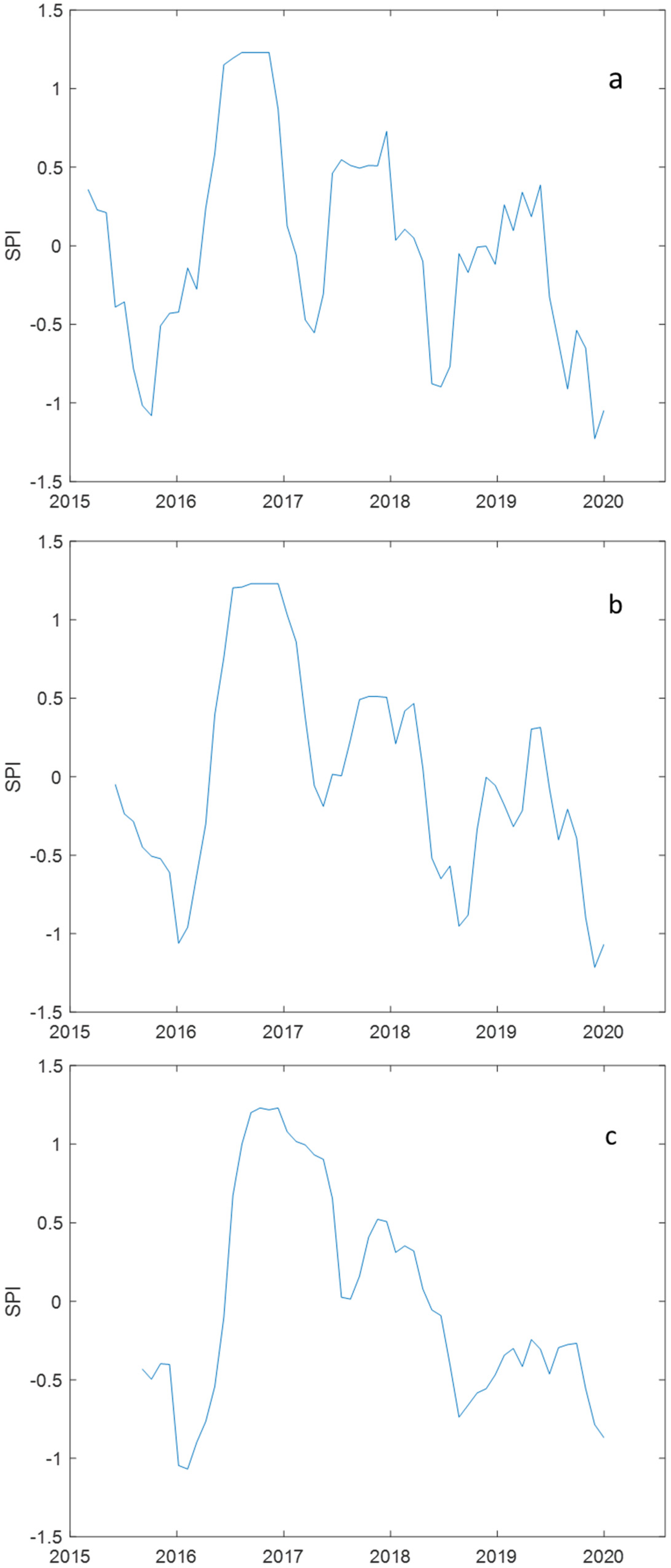
The satellite-based SPI was used to monitor drought condition and measure drought characteristics based on precipitation data. Figure 2 shows the time series of regional SPI 3, SPI 6, and SPI 9 from 2015 to 2019. Different durations of SPI reflected similar drought patterns, but such patterns had different functions. Based on similar SPI results at these time scales in this study, the serious drought severity occurred in 2015, 2018, and 2019. In 2018–2019, the severe drought condition occurred in August and September 2018 and from June to the end of 2019 [28]. The time periods 2014–2015 and 2018–2019 are classified as warm phases of El Niño [29]. The positive IOD in 2019 is the most extreme event over the past 40 years, with cooler-than-normal sea surface temperatures near Java. This IOD alters the temperature and rainfall patterns in the region [30]. In the latter, SPI 6 was selected as the index for a downscaling case as a proxy indicator of medium-term impacts in Java. SPI 3 shows short–medium conditions, whereas SPI 6 shows a medium condition across distinct seasons. If SPI 9 is less than −1.5 then substantial impacts can occur in agriculture [31]. SPI 9 has the smoothest graph compared with SPI 3 and SPI 6 because the more time accumulated, the smoother the graph of values; therefore, the lower the variation in the SPI.
4.2. Performance of Spatial and Nonspatial Downscaling
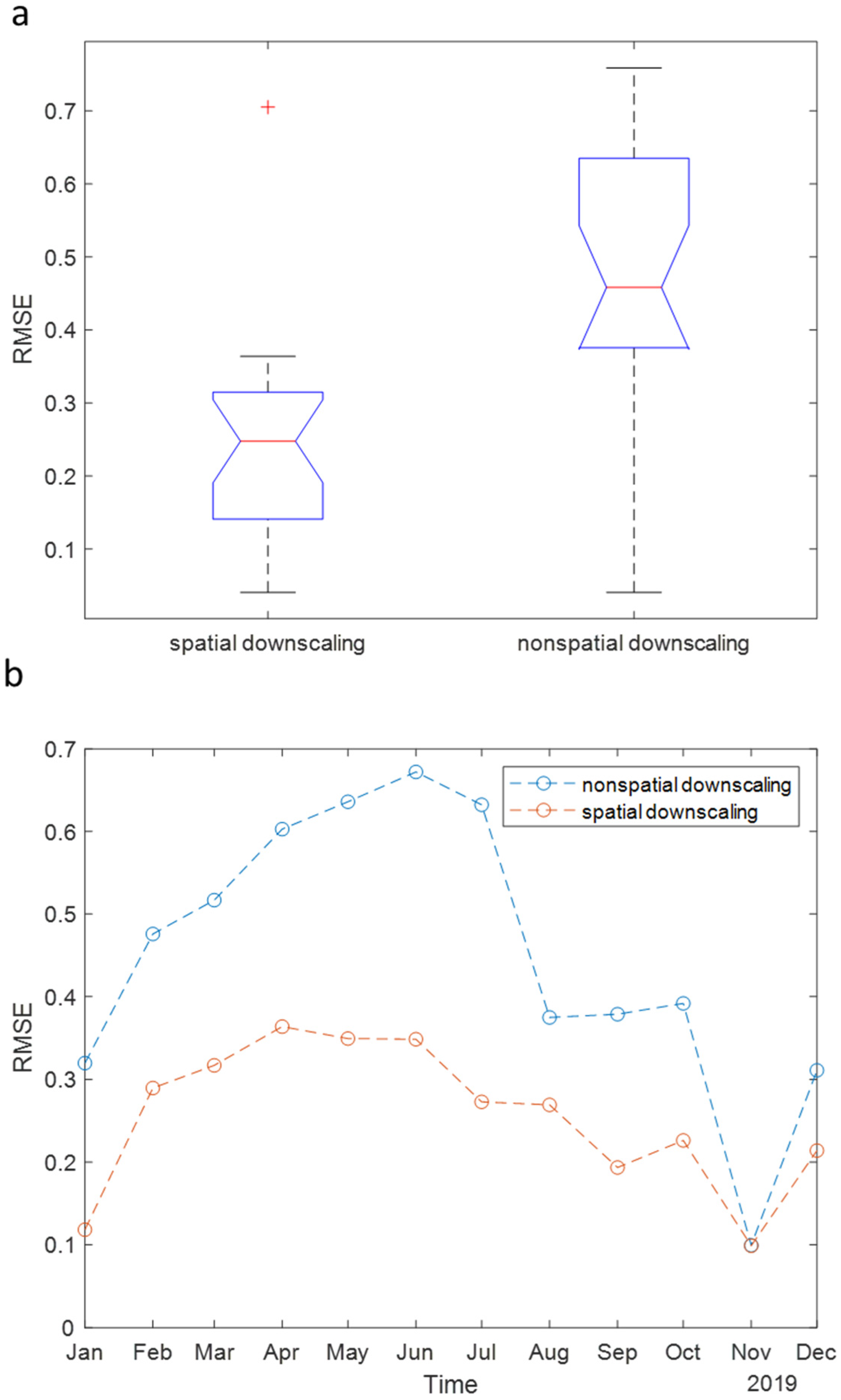
The result shows that the spatial downscaling model of the SPI 6 is superior to the nonspatial downscaling in 2018–2019 (Figure 3a). The mean values of RMSEs in 2018–2019 using spatial and nonspatial downscaling are 0.25 and 0.46, whereas the standard derivation values of RMSEs using spatial and nonspatial downscaling are 0.14 and 0.20. Considering the spatial downscaling model, the model performance is improved because the spatial scheme can generate the spatial-varying function of SPI and environmental observations. Half of the estimation errors can be reduced in spatial downscaling. In addition, the RMSE time series shows that spatial downscaling is better in the transition time for heterogeneous SPI when compared with the whole dry condition (November 2019, Figure 3b).
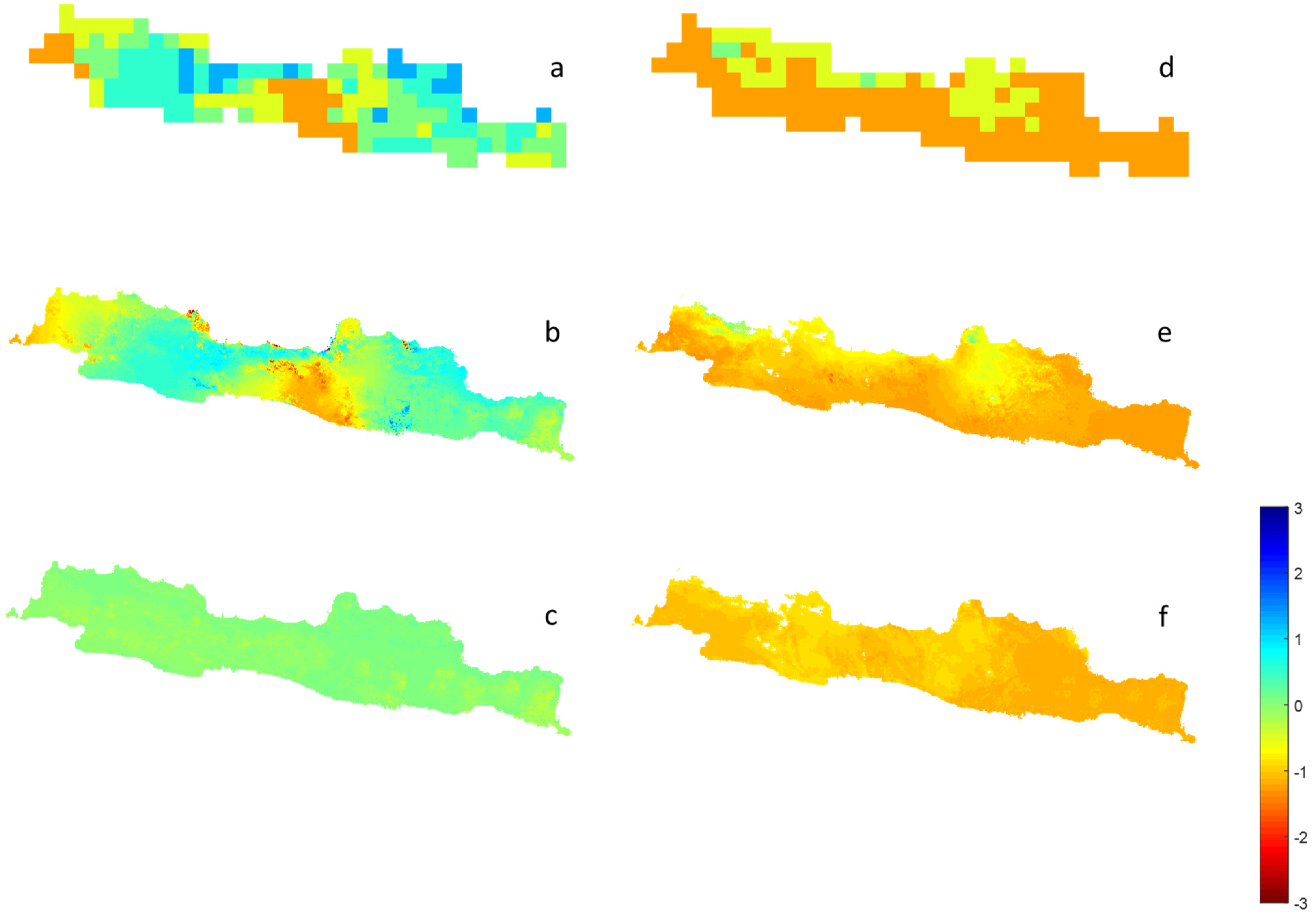
Figure 4 shows the observation and estimation of SPI 6 considering the spatial and nonspatial downscaling in June and December 2019. R values of the spatial and nonspatial downscaling models are 0.863 and 0.137 in June and 0.780 and 0.357 in December, respectively (Figure 4). SPI 6 estimation from spatial downscaling is better than that from nonspatial downscaling, especially in the transition time (June, here). In the nonspatial downscaling model, the estimated SPI in June, 2019 is close to zero whatever the values are from observations. The nonspatial downscaling model cannot catch the spatial variation of the SPI. Figure 5 shows the spatial patterns of original SPI observation from the TRMM data and spatial and nonspatial downscaling results in June (Figure 5a–c) and December (Figure 5d–f) 2019. The pattern of the spatial downscaling model (Figure 5b,e) is similar to that of original SPI (Figure 5a,d) but is more detailed. The result shows that spatial downscaling performs better than nonspatial downscaling (Figure 5c,f), e.g., RMSEs: 0.35 and 0.67 (June) and 0.21 and 0.31 (December) for spatial and nonspatial downscaling in June and December 2019, respectively. Nonspatial downscaling cannot provide any information of drought condition because of heterogenous nature of these variables. However, the nonspatial approach, that is, global linear transformation, can lead to biased estimations of regression model parameters because of the spatial samples [32]. This spatial downscaling approach is a local linear transformation used to model spatially varying relationships. The proposed spatial downscaling model is based on a local weighted fitting approximation to the function being estimated. The model adopted in this study can identify a spatial varying and nonlinear relation between SPI and environmental observations. This research can lead to a comprehensive understanding of the effects of drought using maps.
4.3. Comparison of before and after Downscaling, and SPI Maps of Spatial Downscaling
Figure 6 shows the average and standard deviation values of SPI 6 in 2018–2019 from the original and downscaling data. We have averaged monthly SPI over these years, thereby reducing temporal uncertainties and comparing the results with fine and original spatial resolutions. In general, both data captured similar patterns of SPI 6, e.g., average and standard deviation across Java. As shown in Figure 6a,b most parts of Java showed negative values of average SPI 6, indicating a moderate drought condition. In addition, the western and central parts of Java displayed higher negative values of average SPI 6, which indicated local drought impacts. In addition, the low standard deviation values observed in northwest Java indicated that the observed SPI 6 was consistent (Figure 6c,d). The drought conditions in Java can be identified and monitored based on the statistical description from spatio-temporal patterns of the SPI maps.
Figure 7a–l shows the fine-resolution monthly SPI 6 maps in 2019 using spatial downscaling. The result showed the spatio-temporal patterns of drought conditions in Java. The drought condition in the central Java started from May 2019 (Figure 7e). After July (Figure 7g), the drought condition became the worst. In November 2019 (Figure 7k), drought severity increased in all of Java. Droughts persistent in the dry season from June to November 2019 [28]. Moreover, the fine-resolution SPI maps can be used to understand the details of the drought condition. Based on the results, the drought condition should be managed with caution to ensure Indonesia’s food security and life stability because Java is the main rice-producing island in Indonesia, particularly the central region of the island.
5. Discussion
5.1. Downscaling Model, and Auxiliary Variable Selection
Downscaling refers to an increase of resolution or a decrease in the pixel size of remotely sensed images. Satellite-based precipitation has complete coverage, but fine-resolution precipitation is essential for meteorological, hydrological, and climatology research [16]. Two types of downscaling model can be discerned, such as dynamical model, which account for the different processes within catchments from simulations [33] or statistical models, which accounts for the processes within or across scales [34,35,36,37].
Most satellite precipitation downscaling studies were conducted by considering the auxiliary variables that were highly correlated with precipitation [16]. Auxiliary variables or environmental factors such as NDVI, LST, relative humidity, and geopotential heights were used as predictors; the simulated precipitation values were also considered [34,35]. Moreover, the SPI was highly correlated with the NDVI and LST [38,39], which can be used to forecast drought. Vegetation activity co-varied with remotely sensed meteorological drought along the expected patterns [7]. The relationship between precipitation and vegetation condition was complex [39,40]. Due to the time varying nature of these variables, the time varying downscaling approach is the better choice. Furthermore, rainfall was affected by terrain. In a previous study, a quadratic parabolic equation was used to measure the changes in precipitation with elevation [41]. However, elevation was not considered in this study. The effect of elevation was implicitly considered in this study because LST tended to decline with increasing elevation [42]. Furthermore, current and future satellite missions could develop multi-indicator and composite drought models [6]. Therefore, in the future we will consider more satellite-based variables such as soil moisture in the model [43]. Spatial regression will be available for merging and linking multiple drought-related data into one fine resolution composite map.
5.2. Strength of Time-Varying Spatial Downscaling, and Future Work
The time-dependent spatial regression model estimated the spatial heterogeneity of SPI in each period. The downscaling model developed for this investigation allowed for the spatial patterns of SPI to be estimated solely on the basis of NDVI and LST. The approach is a remote-sensing-based downscaling with spatial-weighted calibration. The model is an effective calibration process for the spatio-temporal mapping and estimation [27,32]. Spatial uncertainty of SPI characteristics can be conducted by spatially varying parameters using spatial regression. The spatial downscaling approach showed better performance when compared with nonspatial downscaling methods. The time-dependent spatial regression model is regarded as a practicable downscaling technique for refining SPI values. This downscaling method is suitable for remote sensing-based regional hydrological and agricultural applications. In this study, the original SPI was calculated based on TRMM data. The regional SPIs reflect reliable patterns of the drought conditions. After SPI downscaling, the fine-resolution SPI with the most serious drought, at transition time or at any time can be identified. The approach is more effective to understand the drought patterns and reduce computing loading. However, considering precipitation downscaling firstly, the SPI will be calculated from fine-resolution precipitation data. The SPI may inherit uncertainty from the massive downscaling data.
Previous studies indicate that precipitation-derived indicators, for example, SPI, are better for drought detection when compared with other indicators for drought early warning [6,38]. Early drought identification is necessary for proactive decision making and disaster preparedness [6]. In this study, the fine-resolution SPI information can be used for early drought detection and drought early warning. This monthly SPI maps provide detailed perspectives of the drought changes, for example, regional characteristics and variations. The drought monitoring is comprehensive for the spatio-temporal dimensions of drought and its severity. Global evaluation of drought indices remains challenging [44]. The global fine-resolution SPI maps will be accomplished in the future. We will effectively evaluate how the environmental effects of drought events evolved [45]. Furthermore, the multiple drought indices or composite drought index will be applied in the future study [46,47].
6. Conclusions
This study aims to refine the SPI maps using a time varying spatial downscaling approach. The SPI each time scale, e.g., SPI 3, SPI 6, or SPI 9 in Java, Indonesia is based on five-year TRMM satellite imagery (0.25° spatial resolution). The 1 km resolution SPI estimation in this study is generated by the time-dependent spatial regression considering the NDVI and LST auxiliary variables from Sentinel-3 images.
The spatial regression is available for linking and merging multiple drought-related data into one fine resolution composite map. Result shows that spatial downscaling was better than nonspatial downscaling (overall RMSEs: 0.25 and 0.46 in spatial and nonspatial downscaling). Considering the spatial function between SPI and environmental variables each period, this study shows that the drought monitoring information from NDVI and LST can be transformed to the fine-resolution SPI. The fine-resolution SPI maps composed of the environmental information match the spatial trend of the original SPI maps. Furthermore, this study detects the temporal drought conditions with fine spatial resolutions in Java Island. The heterogenous SPI patterns are identified by using this spatial downscaling approach when compared with the nonspatial downscaling approach. The spatial downscaling approach reserves the SPI details effectively in the transition time, for example, June 2019 (R: 0.863 and 0.137 in spatial and nonspatial downscaling). Using this model, we can obtain fine spatial resolution information for early drought detection and drought early warning. Moreover, future studies will be applied in the multiple drought indices or composite drought index.
Author Contributions
Conceptualization, H.-J.C.; methodology, R.F.W. and H.-J.C.; validation, R.F.W. and L.M.J.; formal analysis, R.F.W.; investigation, R.F.W.; data curation, L.M.J. and R.F.W.; writing—original draft preparation, H.-J.C.; writing—review and editing, L.M.J. and H.-P.T.; visualization, H.-J.C.; supervision, H.-J.C. and L.M.J. All authors have read and agreed to the published version of the manuscript.
Funding
The study was supported by Ministry of Education, Culture, Research, and Technology, Indonesia (3/E1/KP.PTNBH/2021; 885/PKS/ITS/2021), and Ministry of Science and Technology (MOST), Taiwan (109-2621-M-006 -003-).
Institutional Review Board Statement
Not applicable.
Informed Consent Statement
Not applicable.
Data Availability Statement
Precipitation TRMM data and Sentinel-3 level 2 image products are freely available from NASA and ESA.
Acknowledgments
The authors would like to thank the editors and anonymous reviewers for providing suggestions of paper improvement. We are grateful for the support from SATU joint research scheme and SDGs joint research project in NCKU.
Conflicts of Interest
The authors declare that they have no known competing financial interests or personal relationships that could have appeared to influence the work reported in this paper.
References
- Guttman, N.B. Comparing the palmer drought index and the standardized precipitation index. JAWRA J. Am. Water Resour. Assoc. 1998, 34, 113–121. [Google Scholar] [CrossRef]
- Van Loon, A.F. Hydrological drought explained. Wiley Interdiscip. Rev. Water 2015, 2, 359–392. [Google Scholar] [CrossRef]
- Chu, H.-J. Drought detection of regional nonparametric standardized groundwater index. Water Resour. Manag. 2018, 32, 3119–3134. [Google Scholar] [CrossRef]
- Narasimhan, B.; Srinivasan, R. Development and evaluation of Soil Moisture Deficit Index (SMDI) and Evapotranspiration Deficit Index (ETDI) for agricultural drought monitoring. Agric. For. Meteorol. 2005, 133, 69–88. [Google Scholar] [CrossRef]
- Patel, N.R.; Parida, B.R.; Venus, V.; Saha, S.K.; Dadhwal, V.K. Analysis of agricultural drought using vegetation temperature condition index (VTCI) from Terra/MODIS satellite data. Environ. Monit. Assess. 2012, 184, 7153–7163. [Google Scholar] [CrossRef] [PubMed]
- AghaKouchak, A.; Farahmand, A.M.; Melton, F.S.; Teixeira, J.P.; Anderson, M.; Wardlow, B.; Hain, C.R. Remote sensing of drought: Progress, challenges and opportunities. Rev. Geophys. 2015, 53, 452–480. [Google Scholar] [CrossRef] [Green Version]
- Nicolai-Shaw, N.; Zscheischler, J.; Hirschi, M.; Gudmundsson, L.; Seneviratne, S.I. A drought event composite analysis using satellite remote-sensing based soil moisture. Remote Sens. Environ. 2017, 203, 216–225. [Google Scholar] [CrossRef]
- Wan, Z.; Wang, P.; Li, X. Using MODIS land surface temperature and normalized difference vegetation index products for monitoring drought in the southern Great Plains, USA. Int. J. Remote Sens. 2004, 25, 61–72. [Google Scholar] [CrossRef]
- Weiying, C.; Qianguang, X.; Yongwei, S. Application of the anomaly vegetation index to monitoring heavy drought in 1992. Remote Sens. Environ. 1994, 9, 106–112. [Google Scholar]
- Kogan, F. World droughts in the new millennium from AVHRR-based vegetation health indices. Eos 2002, 83, 557–563. [Google Scholar] [CrossRef]
- Bai, J.-J.; Yu, Y.; Di, L. Comparison between TVDI and CWSI for drought monitoring in the Guanzhong Plain, China. J. Integr. Agric. 2017, 16, 389–397. [Google Scholar] [CrossRef] [Green Version]
- Trenberth, K.E.; Shea, D.J. Relationships between precipitation and surface temperature. Geophys. Res. Lett. 2005, 32, L14703. [Google Scholar] [CrossRef]
- Jia, S.; Zhu, W.; Lű, A.; Yan, T. A statistical spatial downscaling algorithm of TRMM precipitation based on NDVI and DEM in the Qaidam Basin of China. Remote Sens. Environ. 2011, 115, 3069–3079. [Google Scholar] [CrossRef]
- Shi, Y.; Song, L. Spatial downscaling of monthly TRMM precipitation based on EVI and other geospatial variables over the Tibetan Plateau from 2001 to 2012. Mt. Res. Dev. 2015, 35, 180–194. [Google Scholar] [CrossRef]
- Shi, Y.; Song, L.; Xia, Z.; Lin, Y.; Myneni, R.B.; Choi, S.; Wang, L.; Ni, X.; Lao, C.; Yang, F. Mapping annual precipitation across Mainland China in the period 2001–2010 from TRMM3B43 product using spatial downscaling approach. Remote Sens. 2015, 7, 5849–5878. [Google Scholar] [CrossRef] [Green Version]
- Chen, C.; Chen, Q.; Qin, B.; Zhao, S.; Duan, Z. Comparison of different methods for spatial downscaling of GPM IMERG V06B satellite precipitation product over a typical arid to semi-arid area. Front. Earth Sci. 2020, 8, 525. [Google Scholar] [CrossRef]
- Bai, L.; Shi, C.; Li, L.; Yang, Y.; Wu, J. Accuracy of CHIRPS satellite-rainfall products over Mainland China. Remote Sens. 2018, 10, 362. [Google Scholar] [CrossRef] [Green Version]
- Retalis, A.; Tymvios, F.; Katsanos, D.; Michaelides, S. Downscaling CHIRPS precipitation data: An artificial neural network modelling approach. Int. J. Remote Sens. 2017, 38, 3943–3959. [Google Scholar] [CrossRef]
- Neeti, N.; Murali, C.A.; Chowdary, V.; Rao, N.; Kesarwani, M. Integrated meteorological drought monitoring framework using multi-sensor and multi-temporal earth observation datasets and machine learning algorithms: A case study of central India. J. Hydrol. 2021, 601, 126638. [Google Scholar] [CrossRef]
- Lim, E.-P.; Hendon, H.H. Causes and predictability of the negative Indian Ocean dipole and its impact on La Niña during 2016. Sci. Rep. 2017, 7, 12619. [Google Scholar] [CrossRef] [Green Version]
- Dewi, Y.W.; Wirasatriya, A.; Sugianto, D.N.; Helmi, M.; Marwoto, J.; Maslukah, L. Effect of ENSO and IOD on the variability of sea surface temperature (SST) in java sea. IOP Conf. Series Earth Environ. Sci. 2020, 530, 012007. [Google Scholar] [CrossRef]
- Rismayatika, F.; Saraswati, R.; Shidiq, I.P. Taqyyudin identification of dry areas on agricultural land using normalized difference drought index in magetan regency. IOP Conf. Series: Earth Environ. Sci. 2020, 540, 012029. [Google Scholar] [CrossRef]
- Kummerow, C.D.; Simpson, J.; Thiele, O.; Barnes, W.; Chang, A.T.C.; Stocker, E.; Alder, R.F.; Hou, A.; Kakar, A.; Wentz, F.; et al. The status of the tropical rainfall measuring mission (TRMM) after two years in orbit. J. Appl. Meteorol. 2000, 39, 1965–1982. [Google Scholar] [CrossRef]
- Farahmand, A.; AghaKouchak, A. A generalized framework for deriving nonparametric standardized drought indicators. Adv. Water Resour. 2015, 76, 140–145. [Google Scholar] [CrossRef]
- Gringorten, I.I. A plotting rule for extreme probability paper. J. Geophys. Res. Space Phys. 1963, 68, 813–814. [Google Scholar] [CrossRef]
- Ali, M.Z.; Chu, H.-J.; Burbey, T.J. Mapping and predicting subsidence from spatio-temporal regression models of groundwater-drawdown and subsidence observations. Hydrogeol. J. 2020, 28, 2865–2876. [Google Scholar] [CrossRef]
- Chu, H.-J.; He, Y.-C.; Chusnah, W.; Jaelani, L.; Chang, C.-H. Multi-reservoir water quality mapping from remote sensing using spatial regression. Sustainability 2021, 13, 6416. [Google Scholar] [CrossRef]
- Climate Risk Profile: Indonesia 2021. The World Bank Group and Asian Development Bank. Available online: https://climateknowledgeportal.worldbank.org/sites/default/files/2021-05/15504-Indonesia%20Country%20Profile-WEB_0.pdf (accessed on 15 August 2021).
- Historical El Nino/La Nina Episodes (1950–Present). Available online: https://origin.cpc.ncep.noaa.gov/products/analysis_monitoring/ensostuff/ONI_v5.php (accessed on 6 September 2021).
- Meet ENSO’s neighbor, the Indian Ocean Dipole. Available online: https://www.climate.gov/news-features/blogs/enso/meet-enso%E2%80%99s-neighbor-indian-ocean-dipole (accessed on 6 September 2021).
- Pramudya, Y.; Onishi, T. Assessment of the Standardized Precipitation Index (SPI) in Tegal City, Central Java, Indonesia. IOP Conf. Series: Earth Environ. Sci. 2018, 129, 012019. [Google Scholar] [CrossRef]
- Chu, H.-J.; Ali, M.Z.; He, Y.-C. Spatial calibration and PM2.5 mapping of low-cost air quality sensors. Sci. Rep. 2020, 10, 22079. [Google Scholar] [CrossRef]
- Bowden, J.H.; Talgo, K.D.; Spero, T.L.; Nolte, C. Assessing the added value of dynamical downscaling using the standardized precipitation index. Adv. Meteorol. 2016, 2016, 8432064. [Google Scholar] [CrossRef] [Green Version]
- Tatli, H. Downscaling standardized precipitation index via model output statistics. Atmósfera 2015, 28, 83–98. [Google Scholar] [CrossRef]
- Hertig, E.; Tramblay, Y. Regional downscaling of Mediterranean droughts under past and future climatic conditions. Glob. Planet. Chang. 2017, 151, 36–48. [Google Scholar] [CrossRef]
- He, X.; Chaney, N.W.; Schleiss, M.; Sheffield, J. Spatial downscaling of precipitation using adaptable random forests. Water Resour. Res. 2016, 52, 8217–8237. [Google Scholar] [CrossRef]
- Zhang, H.; Loáiciga, H.A.; Ha, D.; Du, Q. Spatial and temporal downscaling of TRMM precipitation with novel algorithms. J. Hydrometeorol. 2020, 21, 1259–1278. [Google Scholar] [CrossRef]
- Bachmair, S.; Tanguy, M.; Hannaford, J.; Stahl, K. How well do meteorological indicators represent agricultural and forest drought across Europe? Environ. Res. Lett. 2018, 13, 034042. [Google Scholar] [CrossRef]
- Gidey, E.; Dikinya, O.; Sebego, R.; Segosebe, E.; Zenebe, A. Using drought indices to model the statistical relationships between meteorological and agricultural drought in Raya and its environs, Northern Ethiopia. Earth Syst. Environ. 2018, 2, 265–279. [Google Scholar] [CrossRef]
- Spracklen, D.V.; Baker, J.C.A.; Garcia-Carreras, L.; Marsham, J.H. The effects of tropical vegetation on rain-fall. Annu. Rev. Environ. Resour. 2018, 43, 193–218. [Google Scholar] [CrossRef]
- Zhang, T.; Li, B.; Yuan, Y.; Gao, X.; Sun, Q.; Xu, L.; Jiang, Y. Spatial downscaling of TRMM precipitation data considering the impacts of macro-geographical factors and local elevation in the Three-River Headwaters Region. Remote. Sens. Environ. 2018, 215, 109–127. [Google Scholar] [CrossRef]
- Peng, X.; Wu, W.; Zheng, Y.; Sun, J.; Hu, T.; Wang, P. Correlation analysis of land surface temperature and topo-graphic elements in Hangzhou, China. Sci. Rep. 2020, 10, 10451. [Google Scholar] [CrossRef]
- Peng, J.; Loew, A.; Merlin, O.; Verhoest, N.E.C. A review of spatial downscaling of satellite remotely sensed soil moisture. Rev. Geophys. 2017, 55, 341–366. [Google Scholar] [CrossRef]
- Hoffmann, D.; Gallant, A.J.E.; Arblaster, J.M. Uncertainties in drought from index and data selection. J. Geophys. Res. Atmos. 2020, 125, e2019JD031946. [Google Scholar] [CrossRef]
- Orimoloye, I.R.; Belle, J.A.; Ololade, O.O. Drought disaster monitoring using MODIS derived index for drought years: A space-based information for ecosystems and environmental conservation. J. Environ. Manag. 2021, 284, 112028. [Google Scholar] [CrossRef] [PubMed]
- Dyosi, M.; Kalumba, A.M.; Magagula, H.B.; Zhou, L.; Orimoloye, I.R. Drought conditions appraisal using geoinformatics and multi-influencing factors. Environ. Monit. Assess. 2021, 193, 365. [Google Scholar] [CrossRef] [PubMed]
- Bushra, N.; Rohli, R.V.; Lam, N.S.N.; Zou, L.; Bin Mostafiz, R.; Mihunov, V. The relationship between the normalized difference vegetation index and drought indices in the South Central United States. Nat. Hazards 2019, 96, 791–808. [Google Scholar] [CrossRef]
Figure 1.
Processing workflow for time varying spatial downscaling SPI maps: (1) pre-processing step; (2) TRMM SPI generation using standardized drought analysis; (3) nonspatial and spatial downscaling; (4) validation and comparison.
Figure 1.
Processing workflow for time varying spatial downscaling SPI maps: (1) pre-processing step; (2) TRMM SPI generation using standardized drought analysis; (3) nonspatial and spatial downscaling; (4) validation and comparison.

Figure 2.
Regional SPI time series from 2015–2019 TRMM monthly data in Java: (a) SPI 3, (b) SPI 6, and (c) SPI 9.
Figure 2.
Regional SPI time series from 2015–2019 TRMM monthly data in Java: (a) SPI 3, (b) SPI 6, and (c) SPI 9.

Figure 3.
(a) RMSE boxplots comparing spatial and nonspatial downscaling of SPI 6 in 2018 and 2019 (during drought periods). (b) RMSE time series comparing spatial and nonspatial downscaling of SPI 6 in 2019.
Figure 3.
(a) RMSE boxplots comparing spatial and nonspatial downscaling of SPI 6 in 2018 and 2019 (during drought periods). (b) RMSE time series comparing spatial and nonspatial downscaling of SPI 6 in 2019.

Figure 4.
Estimation and observation plots of spatial (a,c) and nonspatial (b,d) downscaling of SPI 6 in June (a,b) and December (c,d) 2019.
Figure 4.
Estimation and observation plots of spatial (a,c) and nonspatial (b,d) downscaling of SPI 6 in June (a,b) and December (c,d) 2019.

Figure 5.
Spatial patterns of original SPI 6 (a,d), spatial downscaling (b,e) and nonspatial downscaling (c,f) results in June (a–c) and December (d–f) 2019.
Figure 5.
Spatial patterns of original SPI 6 (a,d), spatial downscaling (b,e) and nonspatial downscaling (c,f) results in June (a–c) and December (d–f) 2019.

Figure 6.
Average (a,b) and standard derivation (c,d) maps of SPI 6 in 2018–2019 when compared with original data (a,c) and spatial downscaling results (b,d).
Figure 6.
Average (a,b) and standard derivation (c,d) maps of SPI 6 in 2018–2019 when compared with original data (a,c) and spatial downscaling results (b,d).

Figure 7.
Monthly fine-resolution SPI 6 maps from January to December (a–l), 2019.


Table 1.
Data information in this study.
| Dataset | Spatial Resolution | Temporal Resolution | Time Period | Sources |
|---|---|---|---|---|
| Precipitation | 0.25° | Monthly | 2015–2019 | TRMM 3B43 |
| NDVI | 1 km | Monthly | 2018–2019 | Sentinel-3 SLSTR |
| LST | 1 km | Monthly | 2018–2019 | Sentinel-3 SLSTR |
Publisher’s Note: MDPI stays neutral with regard to jurisdictional claims in published maps and institutional affiliations. |
© 2021 by the authors. Licensee MDPI, Basel, Switzerland. This article is an open access article distributed under the terms and conditions of the Creative Commons Attribution (CC BY) license (https://creativecommons.org/licenses/by/4.0/).
Share and Cite
MDPI and ACS Style
Chu, H.-J.; Wijayanti, R.F.; Jaelani, L.M.; Tsai, H.-P. Time Varying Spatial Downscaling of Satellite-Based Drought Index. Remote Sens. 2021, 13, 3693. https://doi.org/10.3390/rs13183693
AMA Style
Chu H-J, Wijayanti RF, Jaelani LM, Tsai H-P. Time Varying Spatial Downscaling of Satellite-Based Drought Index. Remote Sensing. 2021; 13(18):3693. https://doi.org/10.3390/rs13183693
Chicago/Turabian StyleChu, Hone-Jay, Regita Faridatunisa Wijayanti, Lalu Muhamad Jaelani, and Hui-Ping Tsai. 2021. "Time Varying Spatial Downscaling of Satellite-Based Drought Index" Remote Sensing 13, no. 18: 3693. https://doi.org/10.3390/rs13183693
Note that from the first issue of 2016, this journal uses article numbers instead of page numbers. See further details here.