Multi-Bernoulli Tracking Approach for Occupancy Monitoring of Smart Buildings Using Low-Resolution Infrared Sensor Array

Abstract

Knowledge about the indoor occupancy is one of the important sources of information to design smart buildings. In some applications, the number of occupants in each zone is required. However, there are many challenges such as user privacy, communication limit, and sensor’s computational capability in development of the occupancy monitoring systems. In this work, a people flow counting algorithm has been developed which uses low-resolution thermal images to avoid any privacy concern. Moreover, the proposed scheme is designed to be applicable for wireless sensor networks based on the internet-of-things platform. Simple low-complexity image processing techniques are considered to detect possible objects in sensor’s field of view. To tackle the noisy detection measurements, a multi-Bernoulli target tracking approach is used to track and finally to count the number of people passing the area of interest in different directions. Based on the sensor node’s processing capability, one can consider either a centralized or a full in situ people flow counting system. By performing the tracking part either in sensor node or in a fusion center, there would be a trade off between the computational complexity and the transmission rate. Therefore, the developed system can be performed in a wide range of applications with different processing and transmission constraints. The accuracy and robustness of the proposed method are also evaluated with real measurements from different conducted trials and open-source dataset.

1. Introduction

Occupancy detection is one of the preliminary requirements of smart buildings where its resolution level varies in different applications. Sometimes, it is enough to know whether a zone has been occupied or not. However, in many cases, such as high-level energy saving via demand-controlled heating, ventilation, and air conditioning (HVAC) systems, it is required to know the number of occupants in different zones and its variation during the day [1,2,3]. There exist many works in the occupancy detection of the building zones using different sensors such as passive infrared (PIR), carbon dioxide (CO₂) concentration, temperature, humidity, and light beam whose main goal is to figure out whether an area of interest (AoI) is occupied or not [4,5]. There are also some efforts to count the number of occupants through sensor fusion techniques over wireless sensor networks (WSNs).

By commercializing the concept of internet-of-things (IoT) in recent years and raising the interest of IoT integration with WSNs for smart building, there has been a remarkable research effort in occupancy monitoring of energy-efficient smart buildings [6]. However, in design of occupancy monitoring systems for smart buildings, occupant’s privacy is a crucial concern. Hence, approaches which utilize sensitive data (e.g., high-resolution visual data) are not suitable. On the other hand, and from the perspective of WSN, there are some constraints such as sensor’s lifetime and implementation cost, which should be taken into account in developing any algorithm integrated into WSNs for edge computing. Moreover, to apply IoT-based wireless protocols such as long range wide-area network (LoRaWAN) or narrow-band IoT (NB-IoT) in smart buildings, it is worth noting that the wireless transmission bandwidth available to a WSN is limited with the low duty cycles. Therefore, to address the above-mentioned requirements of an IoT-based occupancy monitoring via WSN, the computational complexity of detection and tracking algorithms and amount of reporting data by each sensor cannot be high. In this work, our goal is to develop a practical occupancy monitoring system for smart buildings, by considering the implementation challenges and privacy concerns.

2. Related Work and Contribution

Using artificial intelligence techniques, different occupancy detection methods are proposed in [3,7]. Nonetheless, to achieve the reported accuracies in these works, a huge amount of data is collected from different types of sensors such as ambient sound, light, PIR, temperature, humidity, CO₂, and even outside weather information as in [7].

Authors in [8] proposed a probabilistic fusion algorithm for occupancy estimation in different building zones, called PLCount. As the input of their occupancy algorithm, the people flow counts from all sensors are required. However, they have used 3D camera-based counting sensors which violates the privacy of building occupants.

Low-resolution infrared (IR) sensor array, also known as IR camera, is one of the sources of information in occupancy monitoring without any privacy concern. This is also suitable to be utilized in WSNs due to the low power consumption. However, a proper data preprocessing is still needed to be applicable in the IoT-based occupancy monitoring. In [2], an IR camera is utilized together with the optical camera to cover the detection failure of optical camera caused by darkness, optical foreground/background similarities, and partial occlusion. Nevertheless, the usage of optical camera is in contrast of privacy requirement. By using a 16 × 16 IR camera, the authors in [9] developed a counting method of the people appear in the sensor’s field of view (FoV). Their pure image processing counting scheme is based on the blob analysis, when a three-stage morphological algorithm with blob’s area adjustment is proposed to relax the issues of merged blob (due to the close people) and multiple blobs from a single person (i.e., head and hands are detected separately). However, their method is case sensitive and people with different heights might be missed easily since their detected blob areas may lie beyond the predefined range. In [10,11,12], an 8 × 8 IR array by Panasonic, called Grid-EYE [13], is used to record the bird’s eye view of AoI. Due to the computational complexity of the proposed supervised learning based methods in [10,11] and the amount of data to be transferred via wireless networks, they are not feasible for an IoT-based WSN. Moreover, their approaches are to monitor the occupancy within the covered region of each sensor. Based on the deployment height and the size of AoI, one may need several sensors to cover a desired zone which makes counting more challenging due to overlapping FoVs. By using 8 × 8 Grid-EYE, the authors in [12] proposed a method to count the number of people who passed the doorway by leveraging a combination of Otsu’s thresholding and modeling thermal noise distribution. For tracking the body(s) over series of frames, they have defined three features: spatial distance, temperature distance, and temporal distance. Nonetheless, they have considered a doorway where at most two people may pass simultaneously, and it is not suitable for more complicated cases with more passing people in different directions. Moreover, the proposed method is highly related to the detection part. If a person gets missed in one frame, the tracking part may lose it.

In this work, we aim to propose a people flow counting method feasible to be applied by sensor nodes in an IoT-based WSN where above-mentioned implementation constraints are met as well as occupant’s privacy. To do so, low-resolution thermal images, captured by 8 × 8 Grid-EYE IR camera, are used to count the number of people who pass the sensor’s FoV in different directions. The people flow counting of sensor nodes can be then used by other algorithms such as PLCount to monitor the occupancy of different building zones. Therefore, we would like to track the trajectories of unknown number of people which can be treated as multi-target tracking (MTT). The MTT has been one of the active areas of the signal processing for many decades with a wide range of applications, from aerospace to robotic and vehicular fields and even biology. The main objective of MTT is to jointly estimate unknown and time-varying number of targets and their states by using noisy measurements. Among all approaches for MTT, the multi-target Bayesian filtering approach has been developed widely in recent works by applying the concept of random finite set (RFS) for a collection of targets’ states. Moreover, several sequential Monte Carlo (SMC) based approaches have been proposed in [14,15,16] to enhance the performance of systems with joint model selection and tracking problems. To relax the numerical complexity of Bayesian MTTs, some approximations have been proposed, such as probability hypothesis density (PHD) and multi-Bernoulli filters. In [17], a multi-sensor multi-Bernoulli filter is used for group target tracking. However, their method is not strictly a tracker since it cannot provide the target trajectory. When one is talking about the tracking, it is required to distinguish the targets to be able to link each target’s states over the time. Therefore, labeled RFS [18,19] is introduced by Vo et al. to address the requirement of distinguishable targets and to find their trajectories.

In recent works, labeled RFSs have been considered in different visual MTT applications. The authors in [20] have applied labeled RFSs on the tracking of resident space objects (RSOs) via SMC-based multi-Bernoulli filtering framework by assuming that RSOs normally have a few pixels of images in size and they do not have any significant position changes between two consecutive frames. We will see that the position changes of targets are much higher in our case considering the size of FoV, number of pixels, and gait velocity of moving users. In [21], an MTT method within the framework of labeled RFS is presented using high-resolution thermal images. In these works, in addition to their main effort on image processing and pixel assignments of different targets (i.e., detection), the SMC-based tracking approaches increase the computational complexity, especially with a multinomial resampling approach as in [21].

To the best of our knowledge, this work is the first attempt to provide a labeled multi-Bernoulli (LMB) [22] based framework of visual MTT for occupancy monitoring of smart building while the mentioned practical constraints of IoT-based WSNs and privacy concerns are taken into account. Furthermore, although the computational cost of some LMB-based approaches can be high (e.g., cubic in both numbers of hypothesized labels and measurements), we will show that lower complexity of the Gibbs sampling-based LMB framework [23] used in this work is acceptable for our use case.

Throughout this paper, $\mathbb{X}$, $\mathbb{Z}$, and $\mathbb{L}$ are used to denote state, observation, and label spaces, respectively. $\mathbb{R}$ is used to denote the set of real numbers, and $\left|·\right|$ defines the cardinality of a set. We use boldfaced characters to denote vectors and matrices, and the superscript ${\left(·\right)}^T$ denotes matrix transpose.

3. System Model

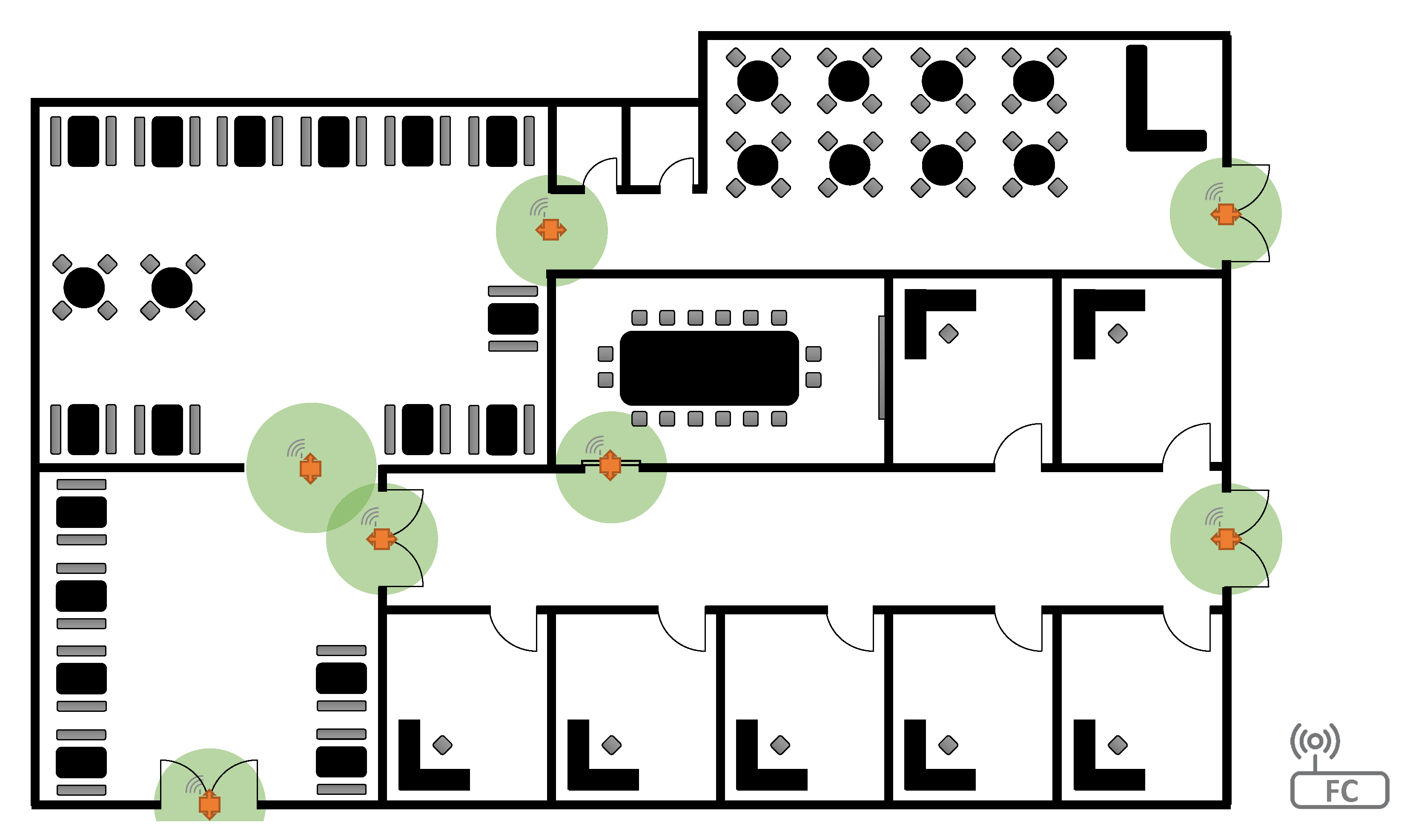
Suppose that a smart building has been divided to different zones and sensors are deployed in their connection points, as shown in Figure 1, where the area of each desired connection point is within FoV of a monitoring sensor. To count the number of people who travel between adjacent zones, each sensor only needs to monitor the people flow passing through connection points in two directions.

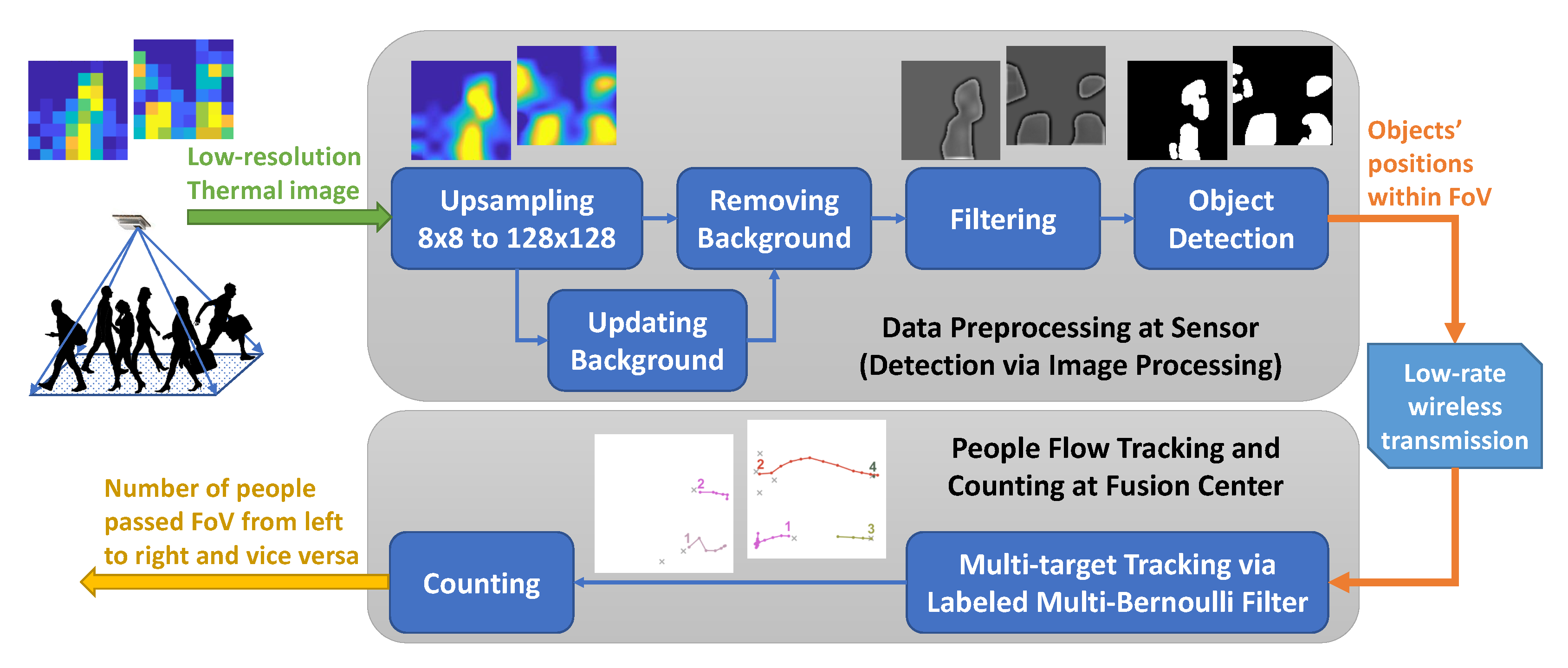
As already discussed, the low transmission rate of wireless communications and low computational capability of the sensors are two fundamental constraints in design of an indoor IoT-based people flow monitoring scheme on the WSN platform where one gets worse to ease the other one. That is, the sensor needs either to send raw/less-processed data (to meet the low computational capability) or to apply high-level data processing algorithms (to transmit a lower amount of data). Since we are talking about the counting of people flow, enough numbers of consecutive measurements are required to track the people in the sensor’s FoV. Considering the walking speed and the deployment height of the sensor (which defines the size of FoV), we may need a measurement rate up to a few frames per second (fps). To meet the occupant’s privacy, we utilize an 8 × 8 Grid-EYE IR array. It means that each sensor node must send 64 thermal values in each transmission, if no data processing is applied in the sensor node. Therefore, as shown in Figure 2, our proposed algorithm consists of two main stages: target detection via thermal image processing and multi-target tracking and counting algorithm. Since sending raw IR data with the enough measurement rate of tracking algorithms needs a high transmission duty cycle [24], the first part is integrated into the sensor to only report a lower amount of data consist of positions of detected objects within the sensor’s FoV. It is worth mentioning that the complexity of the in situ image processing algorithm must be low enough to guarantee the required sensor lifetime, from the perspective of WSNs. This results in erroneous measurements which may contain clutters. The detected positions will be then fed into the tracking algorithm. Although it is supposed that the tracking algorithm is implemented in a fusion center (FC), it is possible to have a full in situ people flow counting if the sensor nodes are capable of performing the tracking algorithm as well. Nonetheless, in this work, we suppose that there is an FC which is responsible to collect reported measurements from all nodes and to monitor the people flow of all building zones. Performing the tracking part in an FC results in a lower implementation cost at the expense of a higher transmission duty cycle of sensor nodes to have the required measurement rates by the tracking algorithm. Therefore, by performing the tracking part either in sensor node or in FC, there would be a trade off between the computational complexity and the transmission rate while both affect the sensor lifetime.

4. Target Detection via Image Processing

As discussed earlier, target detection is the first step to measure the position of possible targets in the scene. At this stage, the main goal is to detect valid objects with different thermal levels from a low-resolution IR image. The body temperature, width, height (which defines distance to the sensor), and cloths (e.g., with or without cap) are some parameters which affect the detection of targets from low-resolution thermal images. Designing an image processing algorithm capable of detecting all possible targets is quite challenging. Even through deep learning (DL) methods, it is not feasible due to the limited computational capability of the sensor nodes in a WSN and necessity of a dataset with a huge number of labeled data. Therefore, in this work, a simple detection method is utilized. The parameters of detecting algorithm and thermal thresholds are chosen to be able to detect objects with lower thermal level (i.e., those who might be short and/or their body temperature is low). In this way, the amount of false alarm (i.e., clutters) increases to reduce the possibility of missed detection. The clutters can then be handled by a proper tracking algorithm.

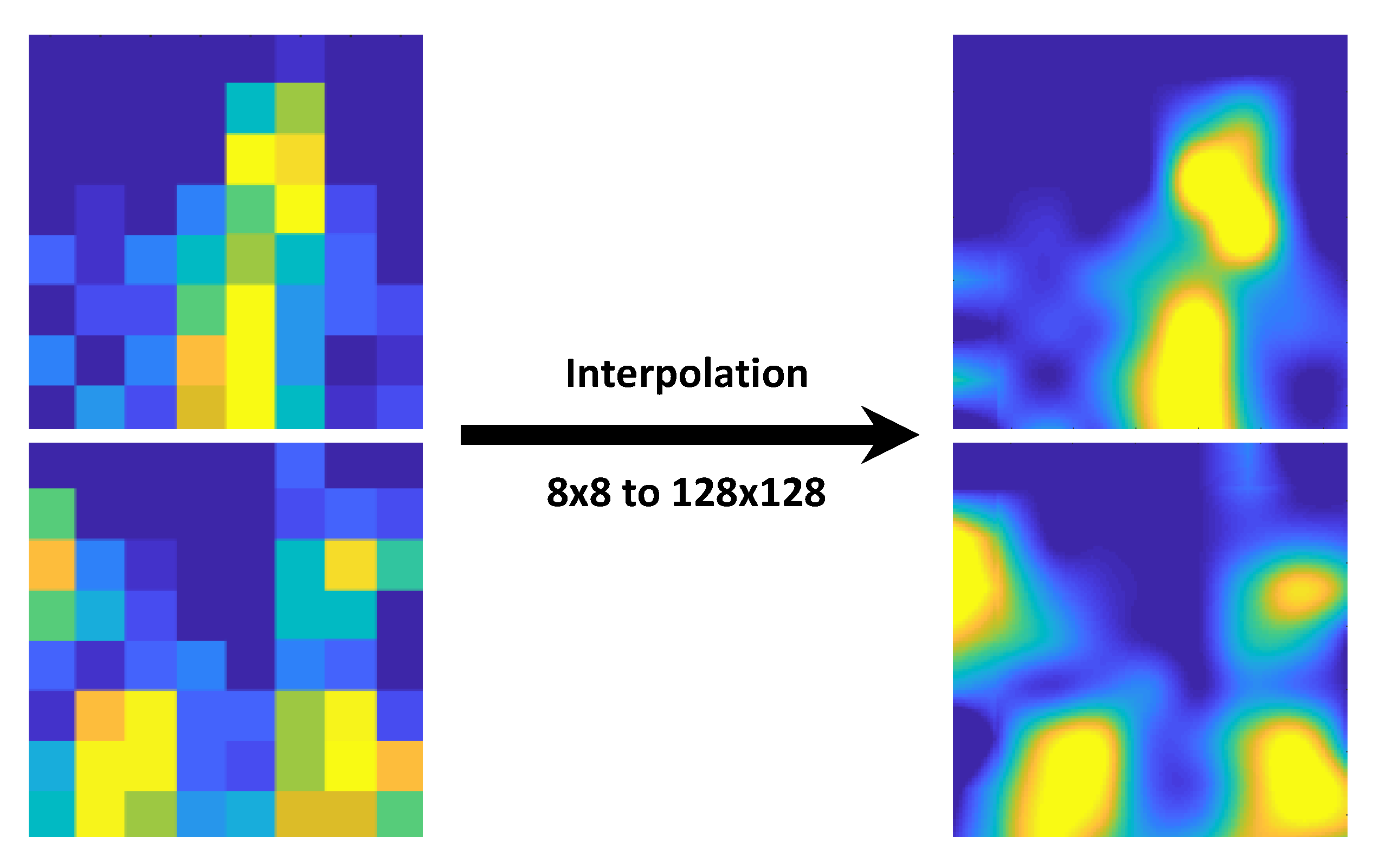
As shown in Figure 2, the low-resolution thermal image is first upsampled, and background image will then be deducted to obtain the foreground image. The update rate of background image is based on environmental changes. It can be scheduled for a predetermined time of the day when the building is empty. The wiser method is to use other motion detectors (e.g., PIR) in vicinity of the sensor and to update the background image when no motion has been detected for a certain period. In addition to the background subtraction, one can also consider a temperature range to have even more reliable foreground thermal image.

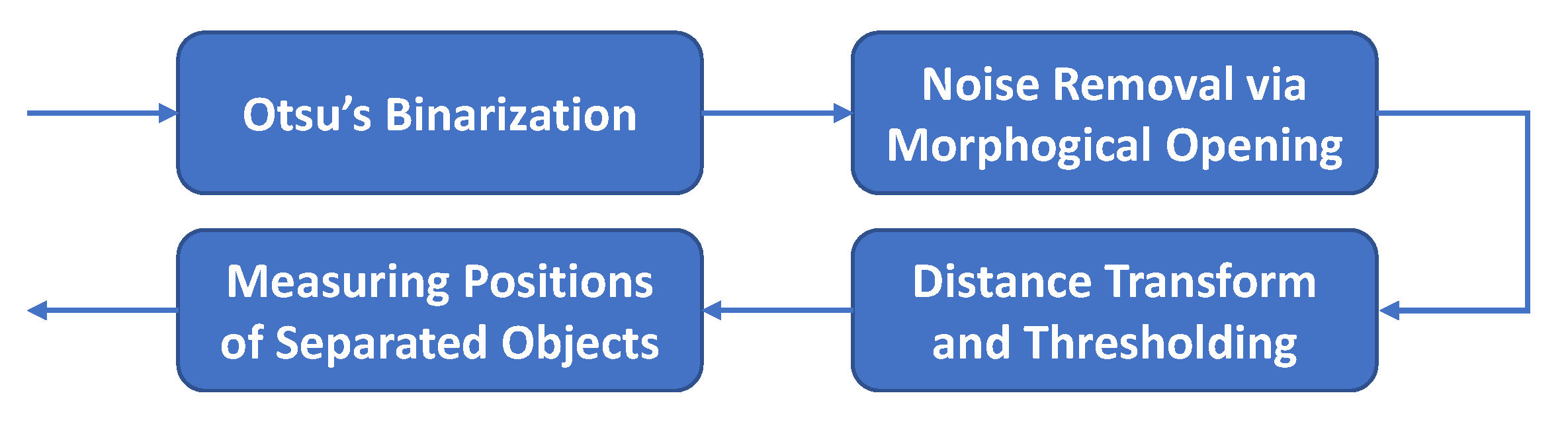
To separate the merged blobs, a Laplacian of Gaussian (LoG) filter is applied on the foreground image. It helps to distinguish passing people who are close to each other [9]. The filtered image is then fed into an object detector. Figure 3 depicts steps of the object detector. After binarization and noise removal, since the boundaries of objects may still touch each other, a distance transformation is applied together with a proper thresholding to have a more clear foreground image. Note that both thresholds, obtained by utilizing Otsu’s method (in binarization) and distance transformation of the binary images, are dynamically updated for each frame. Finally, the central positions of remaining objects in the foreground image are measured and reported.

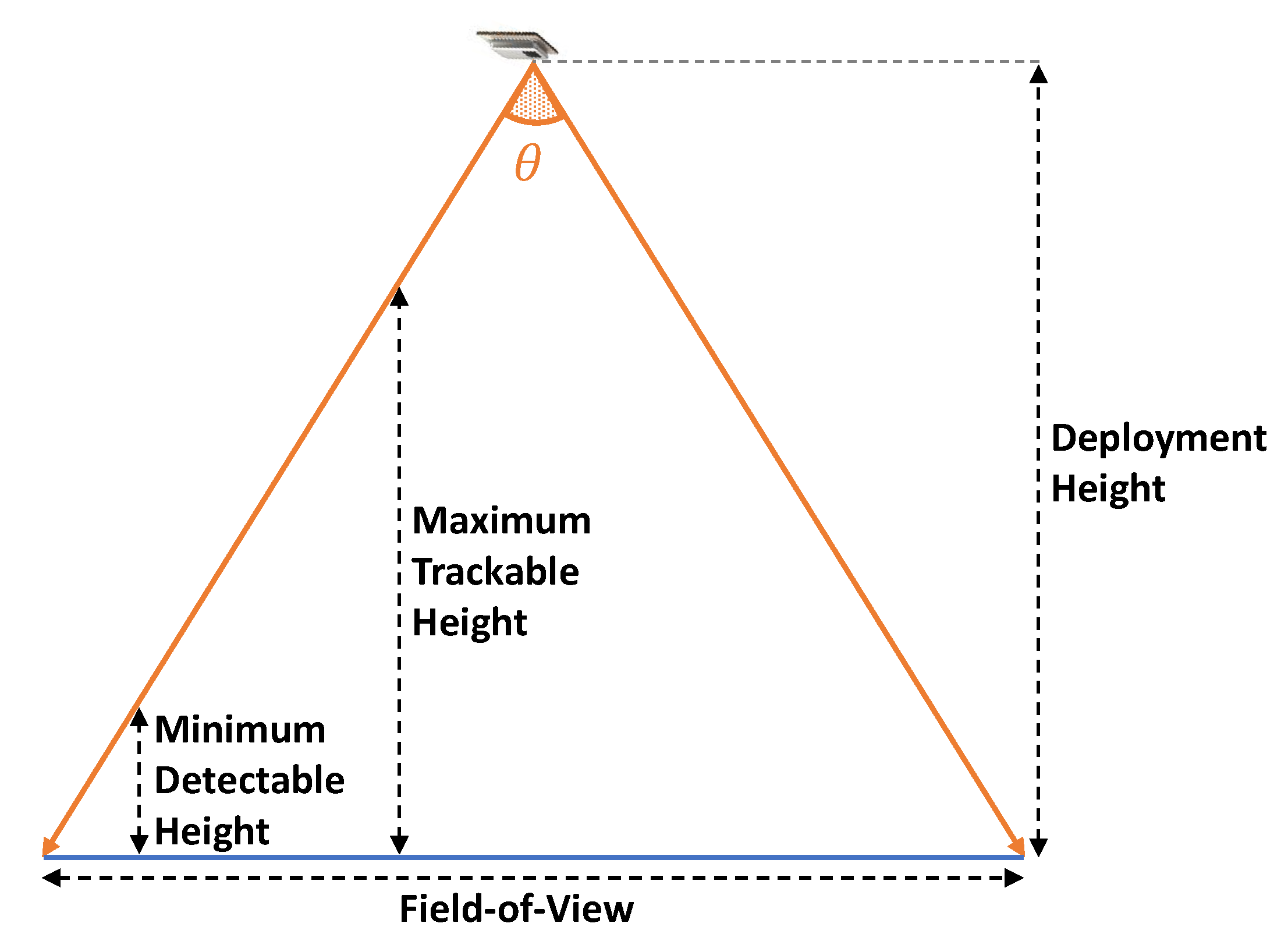
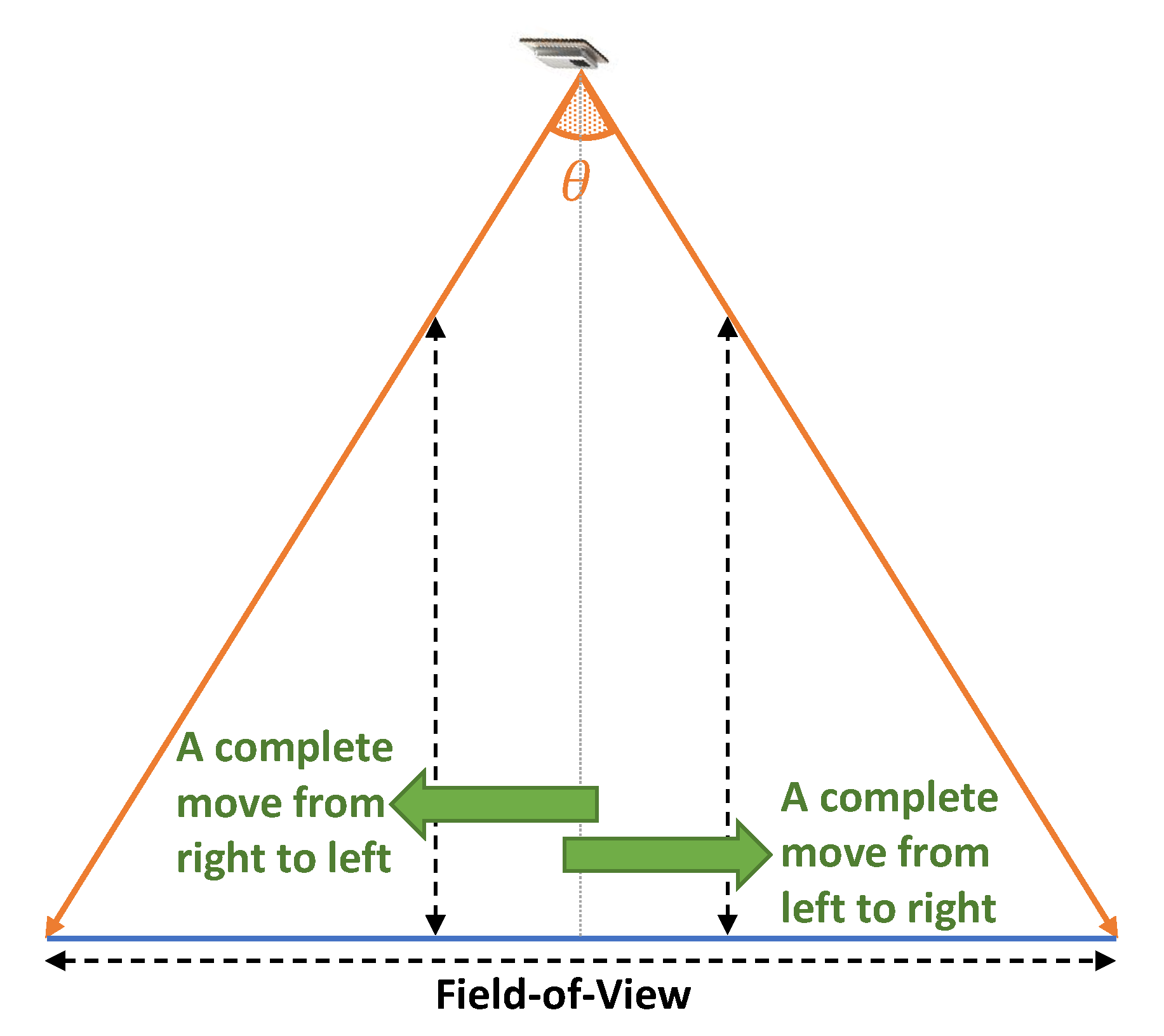
Among the mentioned constraints, the range of target’s height is a key parameter to define the detection parameters and sensor deployment. When the target is too short, its detection is challenging since it is far from the sensor and measured temperature level lies within a lower thermal range [12]. On the other hand, when the target is very tall, it can be easily detected but the number of consecutive frames in which the target appears might be reduced depending on its body temperature, cloths, and walking speed. Therefore, tracking of tall targets would be more difficult since it might be seen as a clutter due the small number of appearances (and being detected) over consecutive frames. It implies that there would be a minimum detectable and a maximum trackable height of target depending on the deployment height of the sensor, as shown in Figure 4. For the minimum detectable height, we may reduce the detection temperature threshold at the expense of more clutters. This issue can be then relaxed by tuning the parameters of tracking algorithm properly. However, the maximum trackable height still remains as a practical constraint, and it can be improved by deploying sensors in a higher ceiling or using sensors with a wider angle of view (AoV), which is defined as $\theta$ in Figure 4.

5. Multi-Target Tracking

To have a reliable tracking algorithm, we need to apply an algorithm which is robust enough to the level of clutters measured and reported by the first detection part. To do so, an LMB filter [22,23] has been utilized for the multi-target tracking part of this work. By using the Gibbs sampling and applying truncation in prediction and update stages jointly, an efficient implementation of LMB with linear complexity in the number of measurements has been introduced in [23]. Therefore, depending on the processing capability of the sensor node, it is possible to integrate the tracking part into the sensor node to have a complete in situ people flow monitoring.

Despite single-target tracking with only one target’s state $x_k\in \mathbb{X}$ at time k, there is a finite set of targets’ states, called multi-target state ${\mathrm{X}}_k=\{x_{k,1},\dots ,x_{k,{\mathcal{N}}_k}\}\in \mathbb{X}$, in the MTT. Note that the number of targets, ${\mathcal{N}}_k$ (also known as cardinality), is an unknown time-varying variable. The multi-target state evolves in time where some targets die (e.g., they leave the AoI) and new targets get born (e.g., they enter the AoI). On the other hand, there is a set of observations, called multi-target observation ${\mathrm{Z}}_k=\{z_{k,1},\dots ,z_{k,{\mathcal{M}}_k}\}\in \mathbb{Z}$, which includes both valid measurements from targets/objects and clutters. Note that there might be some missed detected targets. By treating both multi-target state and multi-target observation as RFSs, it would be possible to develop tracking algorithms based on the concept of Bayesian filtering. Therefore, given the measurement history ${\mathrm{Z}}_{1:k}=({\mathrm{Z}}_1,\dots ,{\mathrm{Z}}_k)$, if a multi-target state is distributed according to $\pi \left(·\right)$, the multi-target posterior at time k is recursively obtained by

$$\begin{array}{c}\hfill {\pi }_{k|k-1}\left({\mathrm{X}}_k\right|{\mathrm{Z}}_{1:k-1})=\int f_{k|k-1}\left({\mathrm{X}}_k\right|\mathcal{X}){\pi }_{k-1}\left(\mathcal{X}\right|{\mathrm{Z}}_{1:k-1})\delta \mathcal{X};\end{array}$$

(1)

and

$$\begin{array}{c}\hfill {\pi }_k\left({\mathrm{X}}_k\right|{\mathrm{Z}}_{1:k})={\displaystyle \frac{g_k\left({\mathrm{Z}}_k\right|{\mathrm{X}}_k){\pi }_{k|k-1}\left({\mathrm{X}}_k\right|{\mathrm{Z}}_{1:k-1})}{\int g_k\left({\mathrm{Z}}_k\right|\mathcal{X}){\pi }_{k|k-1}\left(\mathcal{X}\right|{\mathrm{Z}}_{1:k-1})\delta \mathcal{X}}},\end{array}$$

(2)

as prediction and update stages, where $f_{k|k-1}\left(·\right|·)$ and $g_k\left(·\right|·)$ define multi-target transition model and likelihood function at time k, respectively.

5.1. Labeled Multi-Bernoulli RFS

Based on definition of the Bernoulli trial, a Bernoulli RFS $\mathrm{X}\in \mathbb{X}$ has only two possible cases, $\mathrm{X}\subset \{\varnothing ,x:x\in \mathbb{X}\}$ (i.e., either empty or single-state set), where at most one target’s state can exist with probability r which is distributed based on the probability distribution $p\left(x\right)$. It implies that a Bernoulli RFS has distribution $\pi \left(\mathrm{X}\right)={\delta }_{\{1,|\mathrm{X}\left|\right\}}·r·p\left(x\right)+{\delta }_{\{0,|\mathrm{X}\left|\right\}}·(1-r)$. Note that ${\delta }_{\{·,·\}}$ is Kronecker delta function. Eventually, a multi-Bernoulli RFS can be defined as the union of a finite number of Bernoulli RFSs, $\mathrm{X}={\bigcup }_{i=1}^{\nu }{\mathrm{X}}^{\left(i\right)}$, whose cardinality probabilities, $r^{\left(i\right)}$, and distribution probabilities, $p^{\left(i\right)}\left(x\right)$, are independent. Hence, the probability density of a multi-Bernoulli RFS with n targets’ states from $\nu$ independent Bernoulli RFSs, ${\{r^{\left(i\right)},p^{\left(i\right)}\left(x\right)\}}_{i=1}^{\nu }$, is given by [18], [25] (Page 369)

$$\begin{array}{c}\hfill \pi \left(\{x_1,\dots ,x_n\}\right)=\prod _{j=1}^{\nu }(1-r_k^{\left(j\right)})\sum _{1⩽i_1\ne \cdots \ne i_n⩽\nu }\left(\prod _{j=1}^n{\displaystyle \frac{r^{\left(i_j\right)}{p}^{\left(i_j\right)}\left(x_j\right)}{1-r^{\left(i_j\right)}}}\right),\end{array}$$

(3)

with the summation over all possible permutation of n-variable subsets of a $\nu$-variable set ($n⩽\nu$). The cardinality distribution of a multi-Bernoulli RFS is then obtained by

$$\begin{array}{cc}\hfill \rho \left(n\right)=& \prod _{j=1}^{\nu }(1-r_k^{\left(j\right)})\sum _{1⩽i_1\ne \cdots \ne i_n⩽\nu }\left(\prod _{j=1}^n{\displaystyle \frac{r^{\left(i_j\right)}}{1-r^{\left(i_j\right)}}}\right).\hfill \end{array}$$

(4)

On the other hand, the concept of labeled RFS is introduced for multi-target scenarios to have distinguishable targets where they are marked with unique labels. By considering $\mathbb{X}$ as state space and $\mathbb{L}$ as label space, a labeled RFS is an RFS on $\mathbb{X}\times \mathbb{L}$ with distinct realizations of labels. It is worth noting that the labeling of an RFS does not affect its cardinality distribution since an unlabeled RFS can be easily obtained by discarding the labels from its labeled version [18]. Let $\mathrm{L}\triangleq \mathcal{L}\left(\mathbf{X}\right)$ be the label set of labeled RFS $\mathbf{X}=\{(x_1,{\ell }_1),\dots ,(x_n,{\ell }_n)\}\in \mathbb{X}\times \mathbb{L}$. Hence, $\left|\mathrm{L}\right|=\left|\mathbf{X}\right|$.

Finally, a labeled multi-Bernoulli RFS $\mathbf{X}$ with parameter set $\{(r^{\left(\zeta \right)},p^{\left(\zeta \right)}):\zeta \in \mathsf{\Psi }\}$, is a multi-Bernoulli RFS on $\mathbb{X}$ whose non-empty Bernoulli components are labeled from label space $\mathbb{L}$. Let us define $\alpha :\mathsf{\Psi }\to \mathbb{L}$ as a one-to-one mapping function. Then, for a non-empty Bernoulli component with parameter $(r^{\left(\zeta \right)},p^{\left(\zeta \right)})$, $\alpha \left(\zeta \right)$ provides the label of the corresponding state.

Eventually, the probability density of LMB RFS $\mathbf{X}$ with parameter set $\mathbf{\pi }={\{r^{(\ell )},p^{(\ell )}\}}_{\ell \in \mathbb{L}}$ is given by

$$\begin{array}{c}\hfill \mathbf{\pi }\left(\mathbf{X}\right)={\delta }_{\left\{\right|\mathbf{X}|,|\mathrm{L}\left|\right\}}\prod _{i\in \mathbb{L}}\left(1-r^{\left(i\right)}\right)\prod _{\ell \in \mathrm{L}}{\displaystyle \frac{1_{\{\mathbb{L},\ell \}}{r}^{(\ell )}{p}^{(\ell )}\left(x\right)}{1-r^{(\ell )}}},\end{array}$$

(5)

where

$$\begin{array}{cc}\hfill 1_{\{A,B\}}& \triangleq \left\{\begin{array}{cc}1,\hfill & B\subseteq A;\hfill \\ 0,\hfill & \mathrm{otherwise}.\hfill \end{array}\right.\hfill \end{array}$$

(6)

A general expression of the LMB filter, called generalized LMB (GLMB) filter or Vo-Vo filter, proposed by Vo et al. in [18]. Considering a district index set of components, $\mathbb{C}$, the probability density of a GLMB filter is given by

$$\begin{array}{c}\hfill \mathbf{\pi }\left(\mathbf{X}\right)={\delta }_{\left\{\right|\mathbf{X}|,|\mathrm{L}\left|\right\}}\sum _{c\in \mathbb{C}}{w}^{\left(c\right)}\left(\mathrm{L}\right)\prod _{(x,\ell )\in \mathbf{X}}{p}^{\left(c\right)}(x,\ell )\end{array}$$

(7)

where ${\sum }_{I\subseteq \mathbb{L}}{\sum }_{c\in \mathbb{C}}{w}^{\left(c\right)}\left(I\right)=1$ and $\int p^{\left(c\right)}(x,\ell )dx=1$ are satisfied [22].

By comparing (5) and (7), one can see that the LMB is a special case of GLMB with only one component where

$$\begin{array}{c}\hfill w^{\left(c\right)}\left(\mathrm{L}\right)=\prod _{i\in \mathbb{L}}\left(1-r^{\left(i\right)}\right)\prod _{\ell \in \mathrm{L}}{\displaystyle \frac{1_{\{\mathbb{L},\ell \}}{r}^{(\ell )}}{1-r^{(\ell )}}},\end{array}$$

(8)

and

$$\begin{array}{c}\hfill p^{\left(c\right)}(x,\ell )=p^{(\ell )}\left(x\right).\end{array}$$

(9)

5.2. Tracking via Labeled Multi-Bernoulli Filter

In some tracking applications, like in our case, it is necessary to monitor the target trajectory. Therefore, we need to mark them individually and monitor states of objects with the same mark (label) along the time to observe their trajectories. Therefore, LMB filter has been considered for the tracking part of our algorithm in this work.

One of the main issues of the MTT is data association, where it is difficult to distinguish which observation is related to which target. It is an advantage of the multi-Bernoulli filter-based tracking algorithm that there is no data association requirement. However, its computational complexity increases as the size of measurements goes higher since all survived and possible new born targets will be evaluated and weighted with all measurements at the update stage. Therefore, to relax the computational complexity, especially for the cases with a large number of measurements (which is not our case), Vo et al. have proposed a gating mechanism for the update stage [22], where each target is only evaluated with those measurements whose Mahalanobis distances to the target lie below a certain threshold. In this work, we use the method proposed in [23] where the authors have even improved it by integrating prediction and update stages of the tracking filter to apply only one truncation (instead of truncation at the end of each step) based on the Gibbs sampling. However, some modifications must be applied to fit our use case.

At each timestamp, there are three types of target tracks, those who are newly born (i.e., entered into the FoV at current timestamp), those who survived from the previous timestamp (with an updated state), and those who have just died (i.e., left the FoV).

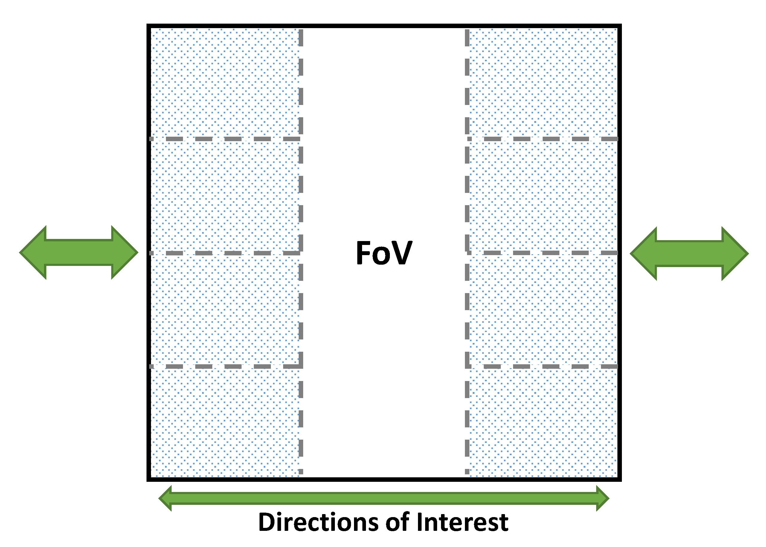
One advantage of utilizing the LMB filter in our use case is that the area of possible birth points is known and limited. The possible target’s birth points of the multi-Bernoulli filter lie within the trackable regions on both sides. Moreover, there is a minimum distance between two people who are walking side-by-side. Considering this minimum distance and the trackable regions, we can define the target’s birth regions as depicted in Figure 5. The number of birth regions depends on size of FoV and the minimum distance between two targets.

Another important difference is related to the possibility of having two people in the same birth region. Obviously, when a target reaches to its exit point, its position would be within one of the birth regions. Therefore, the possibility of having a new born target in that region is low. Hence, we can change weights of any birth in those regions or even omit the related birth points from the RFS. Dropping birth points can reduce the computational time. However, the first option is more reliable since it is still possible to have a new target in that region if big areas are chosen for the birth regions (e.g., two targets might be located in two extreme points of that region) or even a pre-tracked target is wrongly located in a birth region.

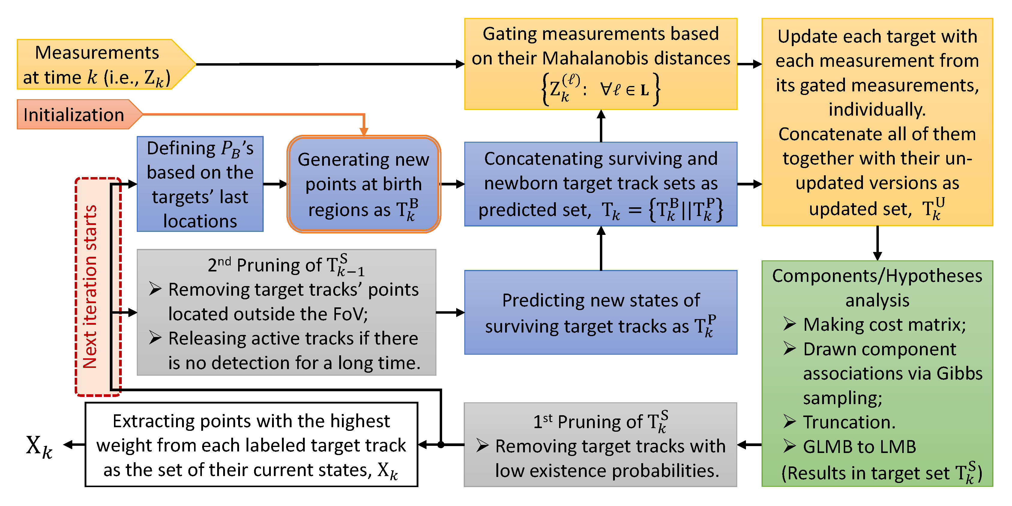
Figure 6 depicts the framework of our LMB-based tracking algorithm while it starts with a set of newborn points, ${\mathrm{T}}_k^{\mathrm{B}}$, (at $k=1$) including their initialized states, existence probabilities, weights, and given labels. For $k>1$, the set of newborn tracks is concatenated with the set of predicted surviving target tracks, ${\mathrm{T}}_k^{\mathrm{P}}$, as a new set, ${\mathrm{T}}_k=\{{\mathrm{T}}_k^{\mathrm{B}}\left|\right|{\mathrm{T}}_k^{\mathrm{P}}\}$. In the next step, all target tracks in ${\mathrm{T}}_k$ are updated with each measurement from their related gated measurements separately. They are then concatenated together and with their un-updated version as a set of updated tracks, ${\mathrm{T}}_k^{\mathrm{U}}$. With the help of Gibbs sampling, a components/hypotheses analysis is applied which results in a set of possible surviving target tracks, ${\mathrm{T}}_k^{\mathrm{S}}$. Note that each component refers to a possible assignment (or combination) of target tracks in ${\mathrm{T}}_k^{\mathrm{U}}$. Finally, the target tracks with the low existence probabilities are dropped in the first pruning attempt. The current states of the desired labeled targets are then extracted from the remain target tracks. The second pruning is applied at the beginning of the next iteration to remove target points located out of the FoV and to release all active tracks if there is no detected point over a predefined number of consecutive measurements. It depends on the data rate and average walking speed within the FoV and must be defined properly to avoid missed detection. This extra pruning is to relax unnecessary computational load of the prediction stage.

A linear Kalman filter (KF) is applied within the structure of an LMB filter. That is the new state of each target from the previous timestamp (as a possible surviving track) is first predicted via a linear transition model individually. They are then updated with the gated observations together with the newly generated birth tracks. In this work, the constant velocity model is considered for the dynamic model because of the low rate of change in speed of moving targets (i.e., change of walking speed) and there is no space to have sudden maneuvers due to the limited FoV. In our test, we observed that it is still able to track those who turn within the FoV since changes in velocities of the target in different directions are tolerable. i.e., ac/deceleration rates in x and y axes are small.

Let ${\tau }_k^{(\ell )}$ be set of histories of association maps for a labeled target track with label ℓ. Suppose that the state of t-th history of a target track with label $\ell \in \mathbb{L}$ at time k is defined as a four-dimensional vector ${\mathbf{x}}_{t,k}^{(\ell )}$, as follows:

$$\begin{array}{c}\hfill {\mathbf{x}}_{t,k}^{(\ell )}\triangleq (x_{t,k},{\ell }_k)\triangleq {[{{}^{\mathrm{x}}p}_{t,k}^{(\ell )},{{}^{\mathrm{y}}p}_{t,k}^{(\ell )},{{}^{\mathrm{x}}v}_{t,k}^{(\ell )},{{}^{\mathrm{y}}v}_{t,k}^{(\ell )}]}^T\in {\mathbb{R}}^4,\forall t=1,\dots ,\left|{\tau }_k^{(\ell )}\right|\end{array}$$

(10)

which includes positions, ${{}^{\left\{\mathrm{x},\mathrm{y}\right\}}p}_{t,k}^{(\ell )}$, and velocities, ${{}^{\left\{\mathrm{x},\mathrm{y}\right\}}v}_{t,k}^{(\ell )}$, of the t-th element of labeled target track ℓ in a two-dimensional plane (i.e., x and y) at time k with covariance $P_{t,k}^{(\ell )}$.

It can then be predicted and updated recursively via a linear KF, as follows:

$$\begin{array}{cc}\hfill x_{t,k|k-1}^{(\ell )}& =f_{k|k-1}\left(x_{t,k-1}^{(\ell )}\right)=\mathrm{F}{x}_{t,k-1}^{(\ell )};\hfill \end{array}$$

(11)

$$\begin{array}{cc}\hfill P_{t,k|k-1}^{(\ell )}& =\mathrm{F}{P}_{t,k-1}^{(\ell )}{\mathrm{F}}^T+\mathrm{Q};\hfill \end{array}$$

(12)

$$\begin{array}{cc}\hfill K_{t,k}^{(\ell )}& =P_{t,k|k-1}^{(\ell )}{\mathrm{H}}^T{(\mathrm{H}{P}_{t,k|k-1}^{(\ell )}{\mathrm{H}}^T+\mathrm{R})}^{-1};\hfill \end{array}$$

(13)

$$\begin{array}{cc}\hfill x_{t|z_j,k}^{(\ell )}& =x_{t,k|k-1}^{(\ell )}+K_{t,k}^{(\ell )}(z_{j,k}^{(\ell )}-\mathrm{H}{x}_{t,k|k-1}^{(\ell )});\hfill \end{array}$$

(14)

$$\begin{array}{cc}\hfill P_{t,k}^{(\ell )}& =P_{t,k|k-1}^{(\ell )}-K_{t,k}^{(\ell )}\mathrm{H}{P}_{t,k|k-1}^{(\ell )},\hfill \end{array}$$

(15)

where

$$\begin{array}{cc}\hfill \mathrm{F}& =\left[\begin{array}{cc}{\mathbf{I}}_2& T_s{\mathbf{I}}_2\\ {\mathbf{0}}_2& {\mathbf{I}}_2\end{array}\right],\hfill \end{array}$$

(16)

and

$$\begin{array}{cc}\hfill \mathrm{H}& =\left[\begin{array}{cc}{\mathbf{I}}_2& {\mathbf{0}}_2\end{array}\right],\hfill \end{array}$$

(17)

are, respectively, dynamic (transition) and observation models in which ${\mathbf{0}}_n$ and ${\mathbf{I}}_n$ represent $n\times n$ zero and identity matrices. The process noise, Q, and measurement noise, R, are given by

$$\begin{array}{c}\hfill \mathrm{Q}={\sigma }_v^2{\Sigma }_n{\Sigma }_n^T,{\Sigma }_n={\left[\begin{array}{cc}{\displaystyle \frac{T_s^2}{2}}{\mathbf{I}}_2& T_s{\mathbf{I}}_2\end{array}\right]}^T,\end{array}$$

(18)

and

$$\begin{array}{c}\hfill \mathrm{R}={\sigma }_z^2{\mathbf{I}}_2.\end{array}$$

(19)

Note that the predicted state of each history element (i.e., $x_{t,k|k-1}^{(\ell )},\forall t=1,\dots ,\left|{\tau }_k^{(\ell )}\right|$) will be updated, separately, with each measurement in the gated observation set of the related labeled target track (i.e., $z_{j,k}^{(\ell )},\forall j=1,\dots ,\left|Z_k^{(\ell )}\right|$). The gated observation set of a target includes all measurements whose Mahalanobis distances to at least one history element of the desired target track is less than a predetermined threshold. Moreover, the resulted RFS (after update stage) includes the un-updated version of all states as well. Let us define ${\mathcal{T}}_k=|{\mathrm{T}}_k|=|{\mathrm{T}}_k^{\mathrm{B}}|+|{\mathrm{T}}_k^{\mathrm{P}}|$ as total number of possibly survived and new born targets. Thus, without the observation gating, the size of RFS would be related to $(1+{\mathcal{M}}_k)\times {\mathcal{T}}_k$ after update stage, where ${\mathcal{M}}_k=\left|{\mathrm{Z}}_k\right|$ is number of observations at time k. It is worth mentioning that each survived target in ${\mathrm{T}}_k^{\mathrm{S}}$ (and then in the predicted set ${\mathrm{T}}_k^{\mathrm{P}}$ in the next iteration) has a set of state(s) history at time k (i.e., ${\tau }_k^{(\ell )}$ for labeled target ℓ) which may include more than one state vector. By applying the observation gating, the size of RFS reduces to

$$\begin{array}{c}\hfill \sum _{\ell \in {\mathrm{T}}_k}(1+|{\mathrm{Z}}_k^{(\ell )}\left|\right)\le (1+{\mathcal{M}}_k)\times {\mathcal{T}}_k,\end{array}$$

(20)

results in a lower computational complexity.

Another parameter, to determine the possibility of survival or death of a pre-detected target at time k, is the existence probability of target track, $r_{k|k-1}^{(\ell )}$, which is predicted based on the survival probability, $P_S$, at each timestamp. For the newborn tracks, it is initialized with the birth probability of the related birth region, $P_B$, as follows:

$$\begin{array}{cc}\hfill r_{k|k-1}^{(\ell )}& =\left\{\begin{array}{cc}{r}_{k-1}^{(\ell )}{P}_S,\hfill & \forall \ell \in {\mathrm{T}}_k^{\mathrm{P}};\hfill \\ P_B,\hfill & \forall \ell \in {\mathrm{T}}_k^{\mathrm{B}}.\hfill \end{array}\right.\hfill \end{array}$$

(21)

As it is already discussed, and shown in Figure 6, $P_B$ is dynamically updated for each region in our tracking algorithm, based on the possibility that a pre-detected target is located close to the related birth region.

Algorithms 1 and 2 depict pseudocodes of prediction and update stages. The weight $w_{t|z_j,k}^{(\ell )}$ is actually the marginal likelihood of observation $z_{j,k}^{(\ell )}$ (given filter parameters), which can recursively be obtained using the last normalized marginal likelihood of the same target’s history, $w_{t,k-1}^{(\ell )}$, and its marginal likelihood ratio for observation $z_{j,k}^{(\ell )}$, $q_{t|z_j,k|k-1}^{(\ell )}$, as follows:

$$\begin{array}{c}\hfill w_{t|z_j,k}^{(\ell )}=q_{t|z_j,k|k-1}^{(\ell )}{w}_{t,k-1}^{(\ell )},\forall t\in {\tau }_k^{(\ell )}\end{array}$$

(22)

where

$$\begin{array}{c}\hfill q_{t|z_j,k|k-1}^{(\ell )}=exp\left\{-0.5d_{z_{j,k}^{(\ell )}}ln\left(2\pi \right)-0.5ln\left(\left|S_{t,k}^{(\ell )}\right|\right)-0.5\left({y_{j,k}^{(\ell )}}^T{S_{t,k}^{(\ell )}}^{-1}{y}_{j,k}^{(\ell )}\right)\right\},\end{array}$$

(23)

in which $d_{z_{j,k}^{(\ell )}}=2$ is the dimension of measurement $z_{j,k}^{(\ell )}$, and

$$\begin{array}{cc}\hfill S_{t,k}^{(\ell )}& =\mathrm{H}{P}_{t,k|k-1}^{(\ell )}{\mathrm{H}}^T+\mathrm{R};\hfill \end{array}$$

(24)

$$\begin{array}{cc}\hfill y_{j,k}^{(\ell )}& =z_{j,k}^{(\ell )}-\mathrm{H}{x}_{t,k|k-1}^{(\ell )},\hfill \end{array}$$

(25)

are innovation covariance and residual.

Algorithm 1: Prediction of the surviving targets.

Algorithm 2: Update using gated observations.

In the next step, by considering all possible cases for each track (i.e., being either not survived, survived but misdetected, or survived and one of detected observations is from that track), a cost matrix is used to draw a few random combinations (associations) of target tracks using Gibbs sampling.

Let us define ${\mathcal{Z}}_k=\left|{\cup }_{\ell \in {\mathrm{T}}_k}{\mathrm{Z}}_k^{(\ell )}\right|$ as total number of measurements used in the update stage. The cost matrix is a ${\mathcal{T}}_k\times (2{\mathcal{T}}_k+{\mathcal{Z}}_k)$ matrix consisting of three parts: The first ${\mathcal{T}}_k\times {\mathcal{T}}_k$ part is related to probabilities of target tracks are not survived (either died or not born). Its diagonal elements are obtained from the non-existence probabilities of the target tracks, i.e., $1-r_{k|k-1}^{(\ell )}$; the second ${\mathcal{T}}_k\times {\mathcal{T}}_k$ part reflects the probability that the target track has been survived but it has not been detected whose diagonal elements are related to the existence probabilities of the track, $r_{k|k-1}^{(\ell )}$, and the missed detection probability of the system, $1-P_D$; and the last ${\mathcal{T}}_k\times {\mathcal{Z}}_k$ part reflects the probability of being survived and detecting whose element in ℓ-th row and j-th column is related to the predictive likelihood of j-th observation being from track ℓ (i.e., $w_{z_j,k}^{(\ell )}$ in Algorithm 2) and clutter intensity as well as existence probabilities of track ℓ and detection probability, $P_D$. One of the drawn target associations would be the case that all targets are supposed to be alive but not detected.

After drawing some combination samples, all possible survived cases (either misdetected or detected and updated with one of the observations) of target track ℓ that have appeared in different combination samples get merged together and form a new set of histories for target track ℓ. Note that each merging case might be a set of histories by itself. States and covariances are merged directly while the weight of each history element is first weighted by cost of its related combination sample before merging. The summation of the weights in the newly formed history set of track ℓ defines its updated existence probability, $r_{k|k}^{(\ell )}$. The marginal likelihoods of the target’s histories at time k, $w_{t,k}^{(\ell )}$, is then obtained by normalizing the weights of histories.

Finally, the new state of target track ℓ (if it is survived) is the state of $t^{\prime }$-th history element which has the maximum marginal likelihood. i.e., $x_k^{(\ell )}=x_{t^{\prime },k}^{(\ell )}$ where $t^{\prime }=\underset{t}{argmax}\left(w_{t,k}^{(\ell )}\right)$.

5.3. Counting

In the counting part of the system, as the final stage of the algorithm, a target’s move from one side to another side is considered complete if it begins before the middle of FoV and ends within the region that lies after the maximum trackable height, as shown in Figure 7. It can be more strict (to avoid false alarm) by considering that the starting point lies in the region which is before the maximum trackable height of the other side. However, it may increase the possibility of misdetection. The choice of starting region depends on the size of FoV and average walking speed.

5.4. Computational Complexity

As discussed earlier, to meet the low processing capability of sensor nodes, a simple image processing algorithm has been considered in the detection stage to avoid high computational complexity. The most complex part of the detection algorithm is Otsu’s thresholding method. However, since low-resolution images are used in this work and it is not aimed to use any high-resolution images due to the privacy concerns, its effect on the total computational complexity is not significant. In the next section, we will show its limited range of processing time since it is not related to the number of targets.

The computational complexity of the implemented LMB-based MTT method in this work is $O\left({\mathcal{T}}^2\mathcal{M}\right)$ which is quadratic in the number of target tracks and linear in the number of measurements [23]. As it is discussed, the limited possible birth points in our case is an important advantage that makes the use of this filter reasonable. The second pruning stage and gated measurements are further attempts to improve the processing time. Note that ${\sum }_{\ell \in {\mathrm{T}}_k}\left|{\mathrm{Z}}_k^{(\ell )}\right|\le {\mathcal{M}}_k{\mathcal{T}}_k$ and the second pruning stage minimizes the size of active target track set ${\mathrm{T}}_k$, ${\mathcal{T}}_k$, by eliminating unnecessary active tracks considering our main goal which is the people flow counting for occupancy monitoring.

6. Experimental Results

To record the required data, Elsys ERS Eye sensors [26] are used which are equipped with 8 × 8 Panasonic Grid-EYE IR arrays. Due to the lack of required network infrastructure and processing capability, the raw data has been recorded in a micro SD card in each sensor at an approximate effective rate of 8 fps. They are then processed off-line.

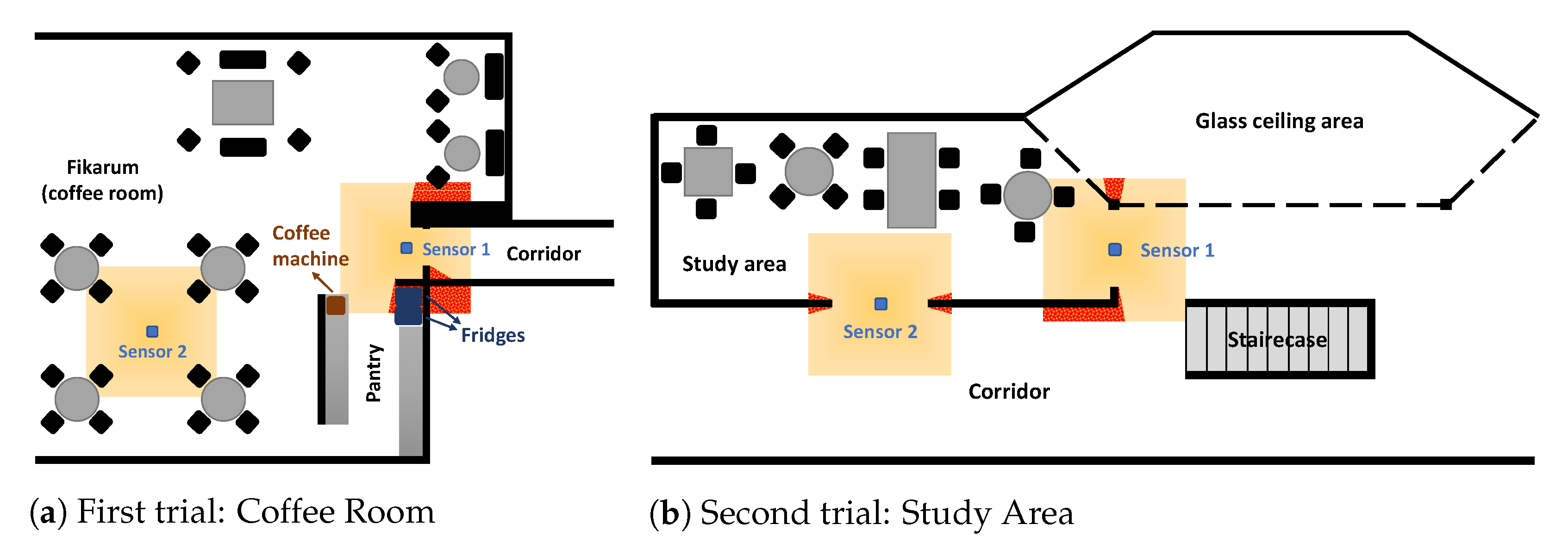
To evaluate the performance of the proposed scheme, two trials have been conducted with different levels of tracking complexity. Figure 8 depicts the layouts and sensor deployments of different trials. Note that the detectable area under each sensor’s FoV is highlighted in Figure 8. They are calculated roughly by considering the deployment height, the 60 degree FoV of sensors, and their maximum detectable distance. The patterned zones are those portions of FoV which are blocked by barriers (e.g., wall or column).

We further analyze the performance of our proposed framework by using an open-source dataset provided by Nagoya University. Finally, the measured processing times will be discussed.

6.1. Coffee Room

In the first trial, a sensor was deployed on the ceiling close to the entrance of the coffee room at department of applied physics and electronics, as shown in Figure 8a. It is not deployed exactly at the entrance (i.e., on or next to the door frame) since the ceiling height is shorter than the minimum required height at the entrance. This trial is considered as the less challenging case due to the following conditions:

• In general, the entry/exit rate is low with the maximum rate during the coffee breaks and lunch time;
• The light intensity of the coffee room was almost constant during the trial since it was lit only by lamps;
• Since the entrance door frame is narrow, users move in a row (when they are more than one) in the majority of the FoV. In the worst case, they may walk side-by-side after or before the entrance door.

However, it has its own challenges. As one may see in Figure 8a, the area around the coffee machine and the fridges, in which the movement is usually high, is within the FoV. Most of the users go directly to that area, after entering the room, to take either coffee or their food from the fridge. They usually spend a few minutes there, either standing or moving. Moreover, some users leave the room after taking coffee with a hot mug in their hand, which might be detected as another user (by target detection part), resulting in more clutters in the measured data.

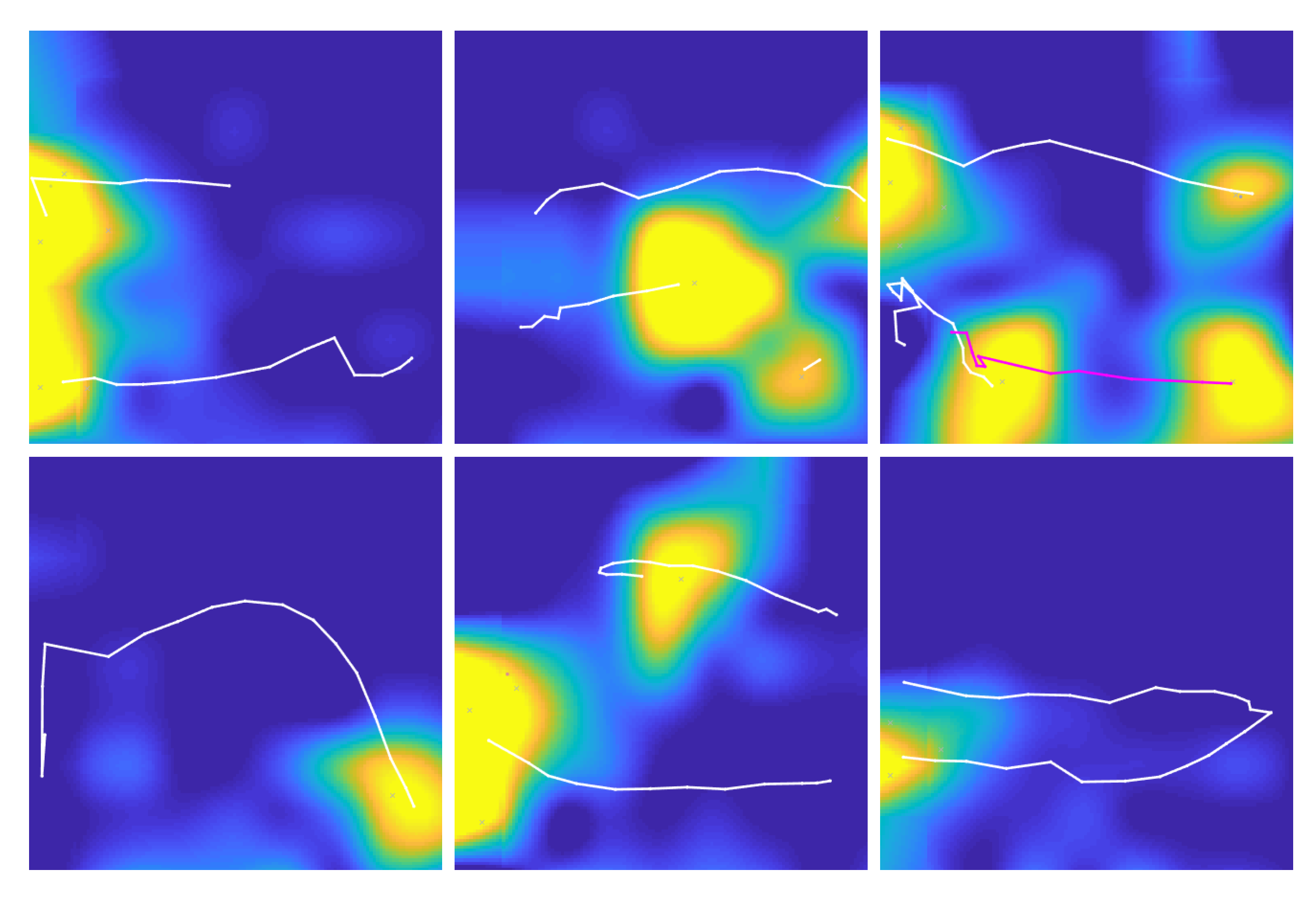
To make it more challenging, another sensor was deployed at the center of coffee room, as depicted as Sensor 2 in Figure 8a, where more users could pass through the FoV simultaneously and towards different directions. We also recorded different infrequent maneuvers, intentionally, for example, walking side-by-side and close to each other, with different walking speeds, diagonal walking, turning at the middle while others are passing FoV, and even when four users are in FoV at the same time walking towards both directions of interest (to simulate concurrent entry and exit). Figure 9 and Figure 10 depict some recorded frames and tracking results of different challenging maneuvers by using Sensor 2 in the coffee room.

For the controlled part (i.e., intentional maneuvers), there were both male and female users with different hair volumes, and their heights were within the range of $1.6$–$1.85$ $\mathrm{m}$.

In this trial, we could count the moving users (i.e., occupancy monitoring) and track different maneuvers (including turning) with an accuracy of 98%.

6.2. Study Area

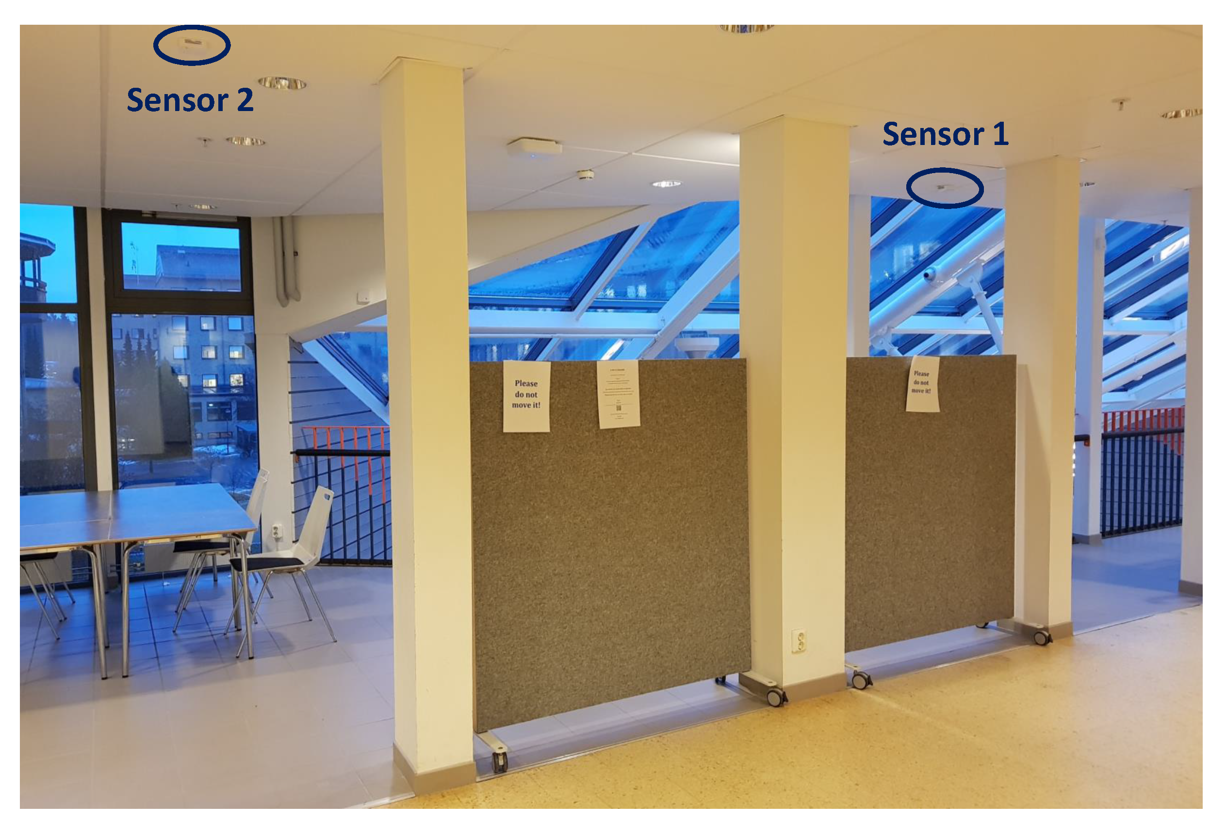
In the second trial, two sensors were deployed on the ceiling at two entrances of a study room at Natural Sciences Building, as shown in Figure 8b and Figure 11. This trial is considered as a more challenging case since

• The occupancy rate of this area is much higher than that of the coffee room;
• The entry/exit rate is also high;
• Some parts of the main corridor and area around the staircase are within the sensors’ FoV, where the movement is too high. Many people pass through those zones without entering or leaving the study area;
• A significant part of the study area is also within the sensors’ FoV. Many students may sit at FoV for a long time. This may increase the tracking error due to the higher clutters;
• Moreover, there is a glass ceiling area where the intensity of direct sun can interfere and reduce the detection ability of Sensor 1 as shown in Figure 11.

The data was collected on different days both in the morning and in the afternoon. The accuracy of tracking algorithm was 86%.

The results can be improved further by using a dynamically updated background data. It can be obtained by using another sensor such as PIR to inform the system when there is no movement in the scene for a predefined period of the time. It also helps to reduce power consumption of the sensor node. In both trials with Grid-EYE IR sensors, a thermal range of 20–$35{}^{°}$C has been considered in the detection stage to obtain more reliable measurements, considering the measurement error provided by the manufacturer in [27]. The chosen range is based on the average temperature of the human skin in indoor environments (considering hairs and cloths) [28,29] and our further investigation in the collected data to ensure that the maximum reasonable range has been considered. In [28] (Section 8.4.1.1), it is stated that “With normal clothing in a room at 15–$20{}^{°}$C, mean skin temperature is 32–$35{}^{°}$C”. Moreover, from [27], the measurement accuracy of the sensor in our operating range is $\pm 2$–$3{}^{°}$C in the worst case (without calibration) which can be reduced to $\pm 0.5$–$1.5{}^{°}$C by calibration.

6.3. Nagoya-OMRON Dataset

To evaluate the robustness of our tracking framework using different senors, we considered a dataset provided by Nagoya University using OMRON 16 × 16 IR array (OMRON D6T-1616L) [30]. This dataset includes low-resolution thermal images of daily human actions such as walking, sitting down, standing up, and falling down which are originally used by authors in [31] for a DL-based action recognition. Since the recorded frames of walking cases are related to our occupancy monitoring framework, they are used to evaluate the performance of our proposed method. Compared to our recorded data, the main differences can be listed as follows:

• A sensor array from another manufacturer is used;
• The original resolution is a bit higher (16 × 16). However, it can still be categorized as the low-resolution IR images;
• They include both dark and light situations;
• In general, the thermal contrast of recorded IR images is lower which results in generating much higher clutters by the image processing part.

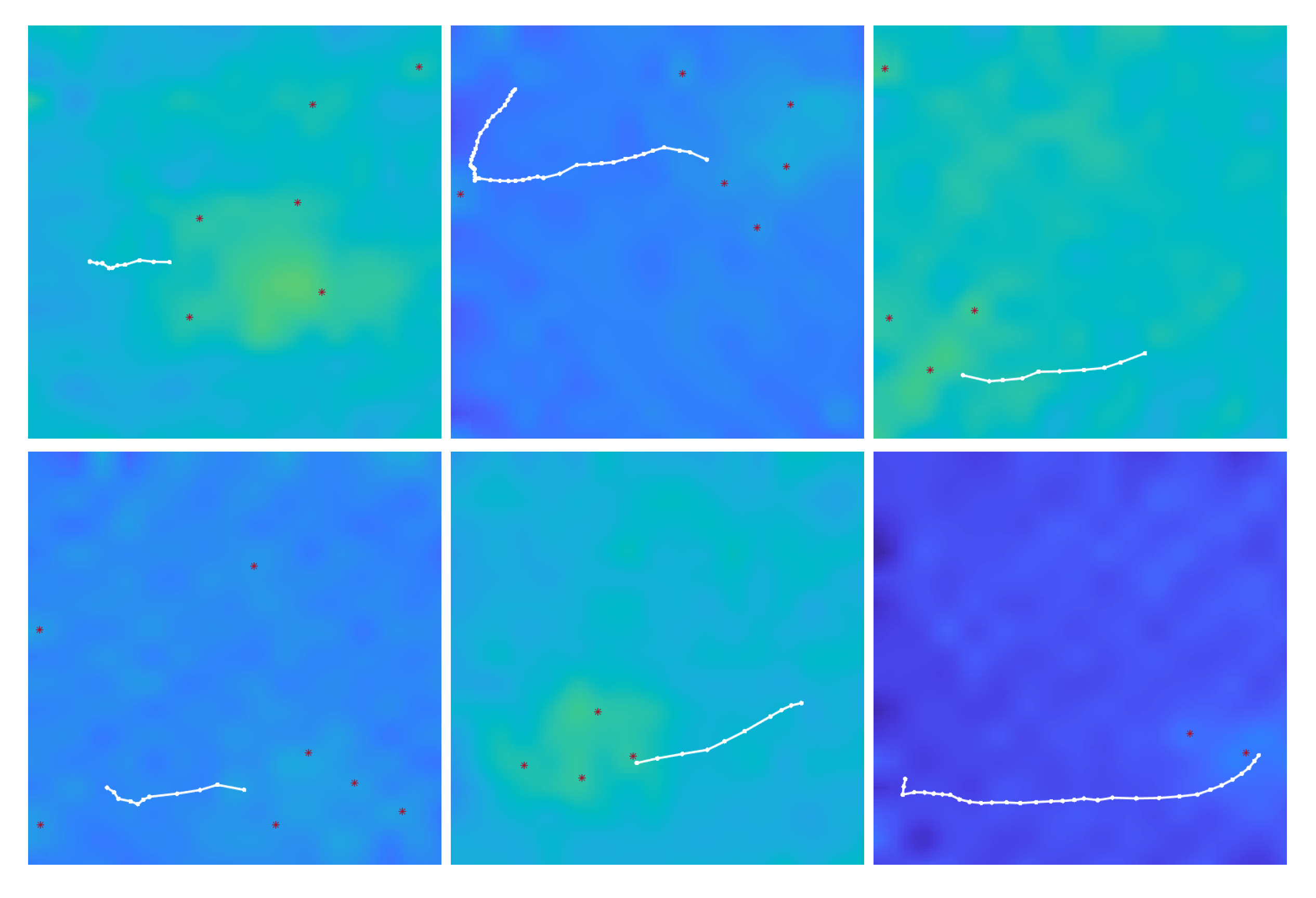
Some recorded frames and related tracking results are shown in Figure 12. From this figure, one can realize the challenges in target detection compared to that of our dataset as shown in Figure 10. Using this dataset, the accuracy of the proposed occupancy tracking method was 87%. It is worth noting that, in [31], their DL-based method has been compared with other methods in which the accuracy of detecting walking action is reported less than 84% when only thermal images are used for classification, a case similar to our framework. However, compared to our dataset, we experienced more false alarms, 3%, which was expected due to the higher clutter rate, and yet, it is still in an acceptable range.

The parameters settings and the performance of proposed people flow monitoring framework on different scenarios are summarized in

Table 1. Parameters settings.

Scenario	IR Array Model	Resolution (pixels)	Height (m)	Rate (fps)	Image Filter	${\mathit{P}}_{\mathit{D}}$ (%)	Min. Targets’ Distance (m)	Max. Trackable Height (m)	${\mathit{\sigma }}_{\mathit{v}}$ (m)	${\mathit{\sigma }}_{\mathit{z}}$ (m)	1st Pruning Threshold (%)	2nd Pruning Det. Gap (no. of Frames)
Coffee Room	Panasonic Grid-EYE	8 × 8	$2.4$	8	LoG	98	$0.7$–$0.75$	2 ${}^{♭}$	1	$0.15$	$0.01$	7
Study Area			$2.65$
Nagoya-OMRON	OMRON D6T-1616L	16 × 16	$2.2$	10	LoG	98	$0.7$–$0.75$	$1.8$	1	$0.22$	$0.01$	3 *

${}^{♭}$ It can be set higher for development height of $2.65$$\mathrm{m}$. However, it is kept 2 $\mathrm{m}$ for the challenging study area to be more safe against the false alarm. * Due to the higher clutter rate in this scenario, the number of invalid tracks increases while the detection gap reduces. Therefore, a shorter period of detection gap is considered to better release unnecessary active tracks.

and

Table 2. Performance of proposed occupancy monitoring method in different scenarios.

Scenario	Detection Accuracy	False Alarm
Coffee Room	98	<1%
Study Area	86	<1%
Nagoya-OMRON	87	3%

, respectively.

Table 3. Performance comparison of different occupancy monitoring methods.

Method	Controlled Environment	Uncontrolled Environment
Proposed Method	98	87
Doorway Method [12]	96	90

compares the accuracy of our method and that of the proposed method in [12] (we call it Doorway method). To do so, the measurements obtained from the controlled trail (i.e., intentional maneuvers recorded by Sensor 2 in coffee room) are evaluated separately, and our uncontrolled measurements in coffee room are evaluated together with the recorded data in study area. From this table, one can see that our tracking system outperforms in the controlled environment while more challenging maneuvers are tracked as explained in Section 6.1. Although the accuracy of Doorway method is about $3\%$ higher than that of our method in uncontrolled situations, their trials are conducted in a shorter duration (totally 6 hrs with many fewer events) in areas whose environmental parameters are more stable compared to our case (e.g., high entry/exit rate and glass ceiling of the study area). Note that the tracking part of the Doorway method is highly dependent to the performance of its detection part in consecutive frames which limits the flexibility of the system in different applications, especially in IoT-based WSNs.

6.4. Processing Time

In this work, both MATLAB 2018b and 2020a are tried on two different PCs with Intel Core i7 processors, one with clock speed of 2.4 GHz (5th Gen.) and the other one with clock speed of 3.2 GHz (8th Gen.). The average CPU time in each frame analysis is calculated in the range of 15–17 $\mathrm{m}\mathrm{s}$ and 35–47 $\mathrm{m}\mathrm{s}$ for detection and tracking steps, respectively. It implies that an average 50–64 $\mathrm{m}\mathrm{s}$ is required for off-line processing of each measured frame by executing non-optimized codes in a normal PC, which is quite enough for an occupancy tracking system with 8–10 fps measurement rate. The required CPU time can be further reduced by code optimization and using lower level programming languages to be suitable for embedded systems with lower processing capacities, in the case of complete in situ processing. If the required processing capability is still higher than that of the sensor node, we can only implement the detection part in the sensor node and let an FC be responsible for the tracking step.

7. Conclusions

In this work, a multi-Bernoulli-based occupancy monitoring scheme has been proposed for the smart buildings using low-resolution IR cameras. Privacy of the occupants and implementation constraints of the IoT-based wireless sensor networks are two main concerns which are tried to be met in the developed method. Sensor nodes with low processing capabilities, due to the required sensor’s lifetime and implementation cost, together with the limited transmission capacity of IoT wireless protocols, available to the reporting sensors, are main challenges which need to be addressed in applications with integration of IoT and wireless sensor networks. In the discussed framework, it is shown that the proposed scheme has potential to be utilized in the applications with the mentioned constraints. We have also conducted two separate experimental trials to evaluate the accuracy of the proposed algorithm in different scenarios. Although the required accuracy depends on the application, the obtained accuracy is still within an acceptable range for many applications of smart buildings such as space utilization management and demand-controlled HVAC systems. The robustness of the tracking framework is further evaluated by applying it on an open-source dataset using a different sensor. As future work, the integration of IR arrays with other sensors can be considered to enhance the performance of the system. One may consider the usage of PIR to improve both the accuracy and the sensor’s lifetime by doing measurement and background update in a more dynamic manner.

References

- Beltran, A.; Erickson, V.L.; Cerpa, A.E. ThermoSense: Occupancy Thermal Based Sensing for HVAC Control. In Proceedings of the 5th ACM Workshop on Embedded Systems For Energy-Efficient Buildings, Rome, Italy, 14–15 November 2013; ACM: New York, NY, USA, 2013. [Google Scholar]
- Cao, N.; Ting, J.; Sen, S.; Raychowdhury, A. Smart Sensing for HVAC Control: Collaborative Intelligence in Optical and IR Cameras. IEEE Trans. Ind. Electr. 2018, 65, 9785–9794. [Google Scholar] [CrossRef]
- Yang, Z.; Li, N.; Becerik-Gerber, B.; Orosz, M. A Multi-sensor Based Occupancy Estimation Model for Supporting Demand Driven HVAC Operations. In Proceedings of the 2012 Symposium on Simulation for Architecture and Urban Design, Orlando, FL, USA, 26–30 March 2012; Society for Computer Simulation International: San Diego, CA, USA, 2012; pp. 2:1–2:8. [Google Scholar]
- Papatsimpa, C.; Linnartz, J. Propagating sensor uncertainty to better infer office occupancy in smart building control. Energy Build. 2018, 179, 73–82. [Google Scholar] [CrossRef]
- Elkhoukhi, H.; NaitMalek, Y.; Berouine, A.; Bakhouya, M.; Elouadghiri, D.; Essaaidi, M. Towards a Real-time Occupancy Detection Approach for Smart Buildings. Procedia Comput. Sci. 2018, 134, 114–120. [Google Scholar] [CrossRef]
- Akkaya, K.; Guvenc, I.; Aygun, R.; Pala, N.; Kadri, A. IoT-based occupancy monitoring techniques for energy-efficient smart buildings. In Proceedings of the 2015 IEEE Wireless Communications and Networking Conference Workshops (WCNCW), New Orleans, LA, USA, 9–12 March 2015; pp. 58–63. [Google Scholar]
- Ekwevugbe, T.; Brown, N.; Fan, D. A design model for building occupancy detection using sensor fusion. In Proceedings of the 2012 6th IEEE International Conference on Digital Ecosystems and Technologies (DEST), Campione d′Italia, Italy, 18–20 June 2012; pp. 1–6. [Google Scholar] [CrossRef]
- Sangoboye, F.C.; Kjærgaard, M.B. PLCount: A Probabilistic Fusion Algorithm for Accurately Estimating Occupancy from 3D Camera Counts. In Proceedings of the 3rd ACM International Conference on Systems for Energy-Efficient Built Environments, Palo Alto, CA, USA, 16–17 November 2016; ACM: New York, NY, USA, 2016; pp. 147–156. [Google Scholar] [CrossRef] [Green Version]
- Berger, M.; Armitage, A. Room occupancy measurement using low-resolution infrared cameras. In Proceedings of the IET Irish Signals and Systems Conference (ISSC 2010), Cork, Ireland, 23–24 June 2010; pp. 249–254. [Google Scholar] [CrossRef] [Green Version]
- Basu, C.; Rowe, A. Tracking Motion and Proxemics using Thermal-sensor Array. arXiv 2015, arXiv:1511.08166. [Google Scholar]
- Yuan, Y.; Li, X.; Liu, Z.; Guan, X. Occupancy Estimation in Buildings Based on Infrared Array Sensors Detection. IEEE Sens. J. 2020, 20, 1043–1053. [Google Scholar] [CrossRef]
- Mohammadmoradi, H.; Munir, S.; Gnawali, O.; Shelton, C. Measuring People-Flow through Doorways Using Easy-to-Install IR Array Sensors. In Proceedings of the 2017 13th International Conference on Distributed Computing in Sensor Systems (DCOSS), Ottawa, ON, Canada, 5–7 June 2017; pp. 35–43. [Google Scholar]
- Panasonic Industry. Infrared Array Sensor—Grid-EYE. Available online: https://eu.industrial.panasonic.com/products/sensors-optical-devices/sensors-automotive-and-industrial-applications/infrared-array (accessed on 6 August 2021).
- Carvalho, C.M.; Johannes, M.S.; Lopes, H.F.; Polson, N.G. Particle Learning and Smoothing. Stat. Sci. 2010, 25, 88–106. [Google Scholar] [CrossRef] [Green Version]
- Urteaga, I.; Bugallo, M.F.; Djurić, P.M. Sequential Monte Carlo methods under model uncertainty. In Proceedings of the 2016 IEEE Statistical Signal Processing Workshop (SSP), Palma de Mallorca, Spain, 26–29 June 2016; pp. 1–5. [Google Scholar] [CrossRef]
- Martino, L.; Read, J.; Elvira, V.; Louzada, F. Cooperative parallel particle filters for online model selection and applications to urban mobility. Digit. Signal Process. 2017, 60, 172–185. [Google Scholar] [CrossRef] [Green Version]
- Zhang, Z.; Sun, J.; Zhou, H.; Xu, C. Group Target Tracking Based on MS-MeMBer Filters. Remote Sens. 2021, 13, 1920. [Google Scholar] [CrossRef]
- Vo, B.T.; Vo, B.N. Labeled Random Finite Sets and Multi-Object Conjugate Priors. IEEE Trans. Signal Process. 2013, 61, 3460–3475. [Google Scholar] [CrossRef]
- Vo, B.T.; Vo, B.N.; Phung, D. Labeled Random Finite Sets and the Bayes Multi-Target Tracking Filter. IEEE Trans. Signal Process. 2014, 62, 6554–6567. [Google Scholar] [CrossRef] [Green Version]
- Javanmardi, M.; Qi, X. Visual tracking of resident space objects via an RFS-based multi-Bernoulli track-before-detect method. Mach. Vis. Appl. 2018, 29, 1191–1208. [Google Scholar] [CrossRef]
- Li, C.; Wang, W. Detection and Tracking of Moving Targets for Thermal Infrared Video Sequences. Sensors 2018, 18, 3944. [Google Scholar] [CrossRef] [PubMed] [Green Version]
- Reuter, S.; Vo, B.T.; Vo, B.N.; Dietmayer, K. The Labeled Multi-Bernoulli Filter. IEEE Trans. Signal Process. 2014, 62, 3246–3260. [Google Scholar]
- Vo, B.N.; Vo, B.T.; Hung, H. An Efficient Implementation of the Generalized Labeled Multi-Bernoulli Filter. IEEE Trans. Signal Process. 2017, 65, 1975–1987. [Google Scholar] [CrossRef] [Green Version]
- Shallari, I.; Krug, S.; O’Nils, M. Communication and computation inter-effects in people counting using intelligence partitioning. J. Real-Time Image Process. 2020, 17, 1869–1882. [Google Scholar] [CrossRef] [Green Version]
- Mahler, R.P.S. Statistical Multisource-Multitarget Information Fusion; Artech House, Inc.: Norwood, MA, USA, 2007. [Google Scholar]
- Elektroniksystem i Umeå AB (ELSYS). Elsys—ERS Eye. Available online: https://www.elsys.se/en/ers-eye/ (accessed on 10 December 2020).
- Panasonic Automotive & Industrial Systems Europe. Grid-EYE Characteristics (2020-10-15). Available online: https://industry.panasonic.eu/components/sensors/grid-eye (accessed on 10 December 2020).
- Freitas, R.A. Nanomedicine, Volume 1: Basic Capabilities; Landes Bioscience: Austin, TX, USA, 1999. [Google Scholar]
- Montgomery, L.D.; Williams, B.A. Effect of ambient temperature on the thermal profile of the human forearm, hand, and fingers. Ann. Biomed. Eng. 1976, 4, 209–219. [Google Scholar] [CrossRef] [PubMed]
- Kawanishi, Y. Nagoya University Extremely Low-Resolution FIR Image Action Dataset (Ver. 2018). Available online: https://www.murase.m.is.nagoya-u.ac.jp/~kawanishiy/en/datasets.html (accessed on 16 December 2020).
- Kawashima, T.; Kawanishi, Y.; Ide, I.; Murase, H.; Deguchi, D.; Aizawa, T.; Kawade, M. Action recognition from extremely low-resolution thermal image sequence. In Proceedings of the 14th IEEE International Conference on Advanced Video and Signal Based Surveillance, Lecce, Italy, 29 August–1 September 2017; pp. 1–6. [Google Scholar]
Figure 1.
Possible sensor deployment (in orange) and their FoVs (green areas) to monitor occupancy of different zones in a smart building using the proposed method.
Figure 2.
People flow monitoring framework.
Figure 3.
Object detection.
Figure 4.
Sensor’s deployment and its corresponding heights.
Figure 5.
Possible birth regions (patterned) within the FoV.
Figure 6.
LMB-based tracking framework.
Figure 7.
Complete target’s trajectory.
Figure 8.
Layout and sensor deployment in different trials.
Figure 9.
Some frames recorded by Sensor 2 in coffee room.
Figure 10.
Some tracking results using Sensor 2 in coffee room.
Figure 11.
The trial’s environmental condition (e.g., sunlight and location of entrances) and sensor deployment in the study area.
Figure 12.
Some tracking results using Nagoya-OMRON Dataset.