Comparison and Evaluation of Different Pit-Filling Methods for Generating High Resolution Canopy Height Model Using UAV Laser Scanning Data

Abstract

As a common form of light detection and ranging (LiDAR) in forestry applications, the canopy height model (CHM) provides the elevation distribution of aboveground vegetation. A CHM is traditionally generated by interpolating all the first LiDAR echoes. However, the first echo cannot accurately represent the canopy surface, and the resulting large amount of noise (data pits) also reduce the CHM quality. Although previous studies concentrate on many pit-filling methods, the applicability of these methods in high-resolution unmanned aerial vehicle laser scanning (UAVLS)-derived CHMs has not been revealed. This study selected eight widely used, recently developed, representative pit-filling methods, namely first-echo interpolation, smooth filtering (mean, medium and Gaussian), highest point interpolation, pit-free algorithm, spike-free algorithm and graph-based progressive morphological filtering (GPMF). A comprehensive evaluation framework was implemented, including a quantitative evaluation using simulation data and an additional application evaluation using UAVLS data. The results indicated that the spike-free algorithm and GPMF had excellent visual performances and were closest to the real canopy surface (root mean square error (RMSE) of simulated data were 0.1578 m and 0.1093 m, respectively; RMSE of UAVLS data were 0.3179 m and 0.4379 m, respectively). Compared with the first-echo method, the accuracies of the spike-free algorithm and GPMF improved by approximately 23% and 22%, respectively. The pit-free algorithm and highest point interpolation method also have advantages in high-resolution CHM generation. The global smooth filter method based on the first-echo CHM reduced the average canopy height by approximately 7.73%. Coniferous forests require more pit-filling than broad-leaved forests and mixed forests. Although the results of individual tree applications indicated that there was no significant difference between these methods except the median filter method, pit-filling is still of great significance for generating high-resolution CHMs. This study provides guidance for using high-resolution UAVLS in forestry applications.

1. Introduction

As an active remote sensing technology, light detection and ranging (LiDAR) can penetrate the canopy to obtain the vertical structure of a forest, and it has been widely used in forest inventory analyses [1,2]. LiDAR has two common data formats: one is the original discrete point cloud, and the other is the spatially continuous raster surface obtained from raw laser points, such as the digital elevation model (DEM) and digital surface model (DSM) [3]. The canopy height model (CHM) is usually constructed by subtracting the DEM from the DSM or by interpolating the normalized point cloud, which is a direct manifestation of the absolute height distribution of the vegetation canopy above the ground [4]. Compared with the original point cloud data, the storage volume of the CHM is smaller, the raster is more convenient to process (there are many fast and mature image processing technologies), and it is more visually friendly and easier to combine with other remote sensing data [5]. At the same time, the CHM also has important value in individual tree crown segmentation, tree height measurement, biomass and stock volume estimation [6,7,8].

In the CHM generation process, a common problem that seriously affected the CHM quality was the unnatural black holes (pits exhibited within the tree crown) distributed in the CHM [7,9]. Data pits are pixels whose heights are significantly lower than those of their neighbours, and these data pits are typically visible in the CHM [10,11]. Many studies have analysed the potential causes of data pits, such as natural intracrown gaps from sparse foliage [12]. Laser beams penetrate the surface of the tree crown and hit the intracrown, trunk or ground [12,13,14], indicating that data pits are also caused by merging multiple flight lines and overlapping laser beams. Simultaneously, pits may even appear in single flight lines at off-nadir scan angles [11]. In addition, the planimetric and vertical errors caused by global navigation satellite system (GNSS) and inertial measurement unit (IMU) measurements also create pits, particularly for small-footprint LiDAR [15,16]. These invalid values will not only greatly reduce the CHM quality but also have a negative impact on the subsequent application of the CHM.

Many studies have claimed that data pits create issues in data. First, pits can affect the visual appearance of the CHM, and it is difficult to recognize the tree crown [9]. Such data will increase the complexity of individual tree crown segmentation [13] and increase the commission and omission errors of tree top detection [17,18]. Most importantly, the height of the canopy surface will be underestimated [10], as will the individual tree height and crown diameter [17,19]. Additionally, using the statistical attributes of these invalid pixels in the noisy CHM to estimate biochemical parameters related to the forest inventory may be inaccurate [9]. To avoid these problems, Reuter et al. [20] suggested detecting and removing problem pixels. Therefore, accurate representations of canopy surfaces are needed to ensure high-quality CHMs.

Researchers have proposed a variety of methods to improve the quality of CHMs. These methods can be divided into two categories: raster-based (post-processing) and point cloud-based (pre-processing). The raster-based method generates the CHM first and then eliminates pits by image filtering algorithms. There are many commonly used global filters that can be used to smooth CHMs, such as mean, median and Gaussian filters [14,21,22,23]. These filters are simple and fast, but the heights of all pixels in the CHM (including normal pixels) are altered, and the size of the kernel lacks sensitivity [7,9]. Ben-Arie et al. [10] used a Laplacian operator to detect data pits and used a median filter (kernel 3 × 3) to replace the pit values in the original CHM. Zhao et al. [24] combined the Laplacian operator and the morphological closing operator to determine and rescue invalid values. Shamsoddini et al. [9] proposed an adaptive mean filter (AMF) to detect and fill pits. Although these local filling algorithms improve the abovementioned problems, the error in the original CHM generation process is not considered [25].

The other category involves direct processing of the point cloud and generation of a pit-free CHM, which is pre-processing. First, some studies have attempted to filter out the part of the point cloud that best represents the canopy surface in the point cloud to construct a CHM. For example, Gaveau and Hill [19] used only first returns to generate CHMs. Leckie et al. [12] used the highest points in each pixel to generate a CHM. Liu et al. [25] used a selection and sorting mechanism followed by spatial interpolation to generate CHMs. Chen et al. [11] used a robust locally weighted regression and robust z-scores to remove pits. Khosravipour et al. [4] generated a series of partial CHMs from different height intervals of the first returns and then combined these CHMs by selecting the maximum value of each corresponding pixel to form the final CHM. Zhang et al. [26] developed a cloth simulation algorithm for constructing a pit-free CHM and used post-processing to rectify the edge of the tree crown. However, first returns may sometimes be false representations of canopy surfaces [9,10] and these processed selections may miss points that represent accurate canopy surfaces [27]. Khosravipour et al. [17] proposed a spike-free method considering all laser returns for generating DSMs, and they found that compared with using only the first return DSM, the accuracy of treetop detection, especially for small trees, was significantly improved. Hao et al. [27] developed a canopy surface point filtering algorithm called graph-based progressive morphological filtering (GPMF), and they found that the CHM generated with the GPMF method produced few pits while retaining canopy details. These methods usually require several parameters to drive the model, and the effect of applying them to specific data sets requires further evaluation.

In recent years, as an emerging remote sensing dataset, unmanned aerial vehicle laser scanning (UAVLS) data have been widely used in the estimation of forest canopy structure and forest parameters in small-scale forest inventories [28,29]. UAVLS can generate data with point densities of 100–300 points per square metre, or even up to 1000 points per square metre, representing a significant increase in point density compared with the data provided by airborne laser scanning (ALS) [30]. High-density point clouds create high-resolution CHMs because the CHM resolution is usually determined by considering the average point cloud density [31]. A high-resolution (~10 cm) CHM can describe the morphological structure of tree crowns in detail [17,32], and more small trees can be seen compared with lower resolution data [7]. However, the high-resolution CHM has more complex height variations [9] and will create more data noise [33,34]. Although a considerable amount of literature focuses on the pit-filling method, to our knowledge, most UAVLS studies ignore this point, and few studies have used the first return [35] and highest point interpolation techniques [33,36,37] to generate CHMs. Moreover, the applicability of the abovementioned pit-free methods in a CHM derived from high-resolution UAVLS requires discussion.

The main purpose of this study is to compare and evaluate the performances of eight different pit-filling methods to generate high-resolution CHMs derived from UAVLS. The most widely used, recently developed and representative CHM generation methods are selected, including the first-echo interpolation method, smooth filtering (mean, medium and Gaussian) method, highest points interpolation method [12], pit-free algorithm [10], spike-free algorithm [17] and GPMF algorithm [27]. Furthermore, this study aimed to select the most representative raster to describe the upper canopy surface to further improve the accuracy of using high-resolution CHM data in individual tree detection and tree height estimation. Finally, we provide guidance for improving the quality of UAV-LiDAR-derived CHMs in forest inventory applications.

2. Materials

To quantitatively and accurately evaluate the differences between different CHM generation methods and the real canopy surface, both simulated and real-world UAVLS point clouds were employed for testing.

2.1. Simulated Data

We used two geometric models to generate simulated point clouds: cone and hemisphere [38]. In the range of 50 m × 50 m, 50 cones and 50 hemispheres are randomly distributed. The geometric surface points are randomly generated according to Equations (1) and (2), and the average point space is 0.08 m.

$$\mathrm{Cone}:\mathrm{z}=l-\frac{\sqrt{x^2+y^2}}{r/l} , x^2+y^2\le r^2$$

(1)

$$\mathrm{Hemisphere}:\mathrm{z}=\sqrt{\left|r^2-x^2-y^2\right|}, x^2+y^2\le r^2$$

(2)

where $x$, $y$ and $z$ are the spatial coordinates of geometric surface points, $r$ is the radius of the cone and hemisphere and $l$ is the height of a cone. The $r$ and $l$ values are set to 1.5–3.5 and 2–6 m, respectively, and a basic height of 2–6 m is added to the simulated geometry. The average height of the cone is 8.6 m, while that of the hemisphere is 8.8 m. If the simulated geometry overlaps horizontally, the highest point in the vertical direction of the overlapped part is retained to ensure that the sunlit part is the crown surface. In addition, ground points with the same density are added to the non-projection area of the simulated geometry, and the z-value of these ground points is set to 0. Thus, two simulated surface points are created (see Figure 1a,b). Moreover, the surface points were interpolated to the reference CHM (CHM_Reference) for subsequent comparison. Then, different proportions (10–60%) of noise points are randomly added below the simulated surface to create pits with different sizes. The final simulated point clouds are shown in Figure 1c,d. It is worth noting that the simulated points do not follow the laser scanning sensor geometry, so the distributions of these under-canopy points will not be distributed as the simulated along vertical strata in real data.

2.2. Real-World Data

2.2.1. Study Area

The study area is the Maoershan Forest Farm, Shangzhi, Heilongjiang Province, Northeast China, ranging from 127°18′0″ to 127°41′6″E and 45°2′20″ to 45°18′16″N (Figure 2). The slope ranges from 5° to 25°, the terrain is high in the south and low in the north and the average altitude above mean sea level is approximately 400 m. The forest type is a typical natural secondary forest of Northeast China that is mainly composed of precious broad-leaved forest, poplar birch forest and oak forest, as well as a small number of coniferous plantations, such as Korean pine, larch and Scotch pine. In this study, a total of 3 sites, which represent three forest stand types (broadleaf forest, coniferous forest and coniferous and broad-leaved mixed forest), were established.

2.2.2. UAV-LiDAR Data

The UAV-borne LiDAR equipment used in this study was an extremely lightweight RIEGL mini VUX-1UAV LiDAR scanner (www.riegl.com/products/unmanned-scanning/riegl-minivux-1uav, accessed on 8 June 2021) carried by a Feima D200 UAV platform (www.feimarobotics.com/en/productDetailD200, accessed on 8 June 2021). The laser scanner operated at a pulse repetition rate of 100 kHz with scan speeds up to 100 scans per second. The maximum measurement range is 250 m and the range measurement accuracy is 15 mm. The footprint size is 160 mm × 50 mm at 100 m and the beam divergence is 1.6 × 0.5 mrad. The field of view is up to 360° and the angle measurement resolution is 0.001°. The scanner has multiple target capabilities and can generate up to 5 target echoes per laser shot. In addition to the laser sensor, the UAV platform is also composed of a GNSS antenna, a high-precision inertial measurement unit (IMU) and a high-speed storage control unit (see Figure 2). Three parallel batteries ensure the safe landing although two out of three are off, which could support a 48 min hover.

UAVLS data were acquired in August 2019 at three sites. All flights were designed as crossing transects with 80 m swath overlaps at 80 m altitude and 5.0 m/s speed. The average point density for each site ranged from 150 to 250 pt/m². The point clouds of these three sites are shown in Figure 2.

2.2.3. Field-Measured Data

Three 100 m × 100 m plots were established across three sites. Each plot was divided into 25 square sample subplots measuring 20 m × 20 m, and a total of 75 subplots were obtained. The height of all trees in each subplot was measured using a Vertex IV instrument with a height resolution of 0.1 m (Haglöfs, Sweden). Four corners of each subplot were determined with a real-time kinetic (RTK) GNSS (UniStrong G10A, Beijing, China) with a positioning error of approximately 0.1 m. The tree coordinates were recorded by measuring their relative positions from the edges of the subplots by using a hand-held laser rangefinder. Finally, 1456, 1157 and 1372 trees were observed among the three plots. The average heights of Plot 1, Plot 2 and Plot 3 were 12.7 m, 12.5 m and 12.5 m, respectively, and the standard deviations were 3.3 m, 4.0 m and 5.2 m, respectively.

3. Methodology

3.1. UAVLS Data Pre-Processing

The raw UAVLS data are processed by a series of noise removal processes to remove many air points, points below the ground and isolated points in the canopy [29]. Air points and low points were removed manually, and isolated points were determined by the number of points inside the search neighbourhood for a given search radius (5 m). Subsequently, the remaining points were classified into ground and nonground points using the progressive triangulated irregular network (TIN) densification method developed by Axelsson [39]. Then, the ground points were interpolated into a digital terrain model (DTM) using kriging interpolation with a 1 m pixel size [40]. According to the DTM, the average slopes of the three sites were approximately 9°, 11° and 7°. The normalized height of point clouds was obtained by subtracting the DTM value from the elevations of all points [41].

3.2. Description of CHM Generation Algorithms

The most widely used, recently developed and representative eight pit-filling methods are selected to generate CHMs, including the first-echo (FE) interpolation method, smooth filtering (mean, medium and Gaussian) method, highest point (HP) interpolation method [12], pit-free algorithm [10], spike-free algorithm [17] and GPMF algorithm [27]. The smooth filtering method and pit-free algorithm are post-processing methods, while the other four methods are pre-processing methods. Figure 3 shows the process of generating CHMs by these eight methods. FE interpolation is a common CHM generation method that is generated by interpolating all the first echoes in the normalized point cloud. Then, the mean filter, median filter and Gaussian filter are used to smooth the FE CHM. HP interpolation first generates 0.1 m grid cells and then extracts the highest point of each cell for interpolation. The pit-free method, spike-free method and GPMF method are described below.

3.2.1. Pit-Free Algorithm

The pit-free method is a semiautomated pit-filling algorithm that uses a user-defined threshold to detect pits and automatically fill them. Specifically, a Laplacian operator is first applied to the FE CHM and a percentage of the cumulative histogram of the Laplacian image is defined to determine the percent of pits. Then, the data pits are marked as one and the non-data pits are marked as zero to generate a binary mask. At the same time, a median filter (kernel 3 × 3) is used to smooth the FE CHM to generate a pit-filled CHM. Finally, the pixel marked data pits (one) were replaced with the corresponding 3 × 3 median filter CHM value, while the non-data pits (zero) were retained as the original value of the FE CHM.

3.2.2. Spike-Free Algorithm

This algorithm uses all laser returns to generate a TIN and then rasterizes it. The TIN generation starting from the HP and the Delaunay triangle increment is constrained by the lengths of triangle edges and vertical spaces of returns, which suggests that triangles with small edges are more relevant for accurately representing the canopy surface than those with long edges in TIN. Hence, the triangles satisfying the three edge constraints (“freeze distance”) will be frozen in the Delaunay triangle increment. If the elevation of the next candidate point is smaller than the elevation of the triangle, it will be ignored to prevent the appearance of pits. To prevent the triangle from being frozen in advance and causing the pits to be overfilled, a height threshold called the “insertion buffer” is introduced. Before the triangle freezes, the insertion buffer defines a vertical zone to ensure that all triangles that still have points in the buffer will not be frozen. Thus, freeze distance and insertion buffer jointly determine the generation of a spike-free TIN.

3.2.3. Graph-Based Progressive Morphological Filtering

This algorithm uses an adaptive morphological operation to filter surface points from all normalized points in progressive filtering. First, a graph is constructed from all normalized points to model the relationships within these points. Second, adaptive morphological filtering is used to “pull up” the depression in the graph. In general, the more depressed the connected neighbourhoods of points in the graph are, the more likely there are data pits. A sharpness index (SI) is introduced to quantify concave tapering and construct the alterable height threshold adaptive to the spacing value between a certain point and its neighbourhood. The adaptive height threshold in graph-based morphological filtering can filter out non-surface points. Then, a progressive process is conducted to improve the adaptive morphological filter for eliminating spikes of various sizes until no points are excluded. The remaining points are regarded as canopy surface points. Finally, the pit-filled CHM is generated by interpolating the surface points.

To avoid errors caused by spatial interpolation methods, all methods used linear interpolation to generate CHMs. According to previous studies, the spatial resolution of a CHM is finer than one-fourth of the crown diameter [33], and it is determined by considering the mean point space [31,42,43]. In our study, the minimum pulse density was approximately 150 pulses/m², which corresponds to a point spacing of 0.08 m. Therefore, the resolution of the CHM was set to 0.1 m. All subsequent processing was performed on the basis of CHM with 0.1 m resolution. The performance of the pit-free method was analysed by the graphical user interface (GUI) developed by Ben-Arie et al. [10], and the other methods were coded in MATLAB R2019b.

3.3. Accuracy Assessment

First, the CHM quality can be judged by its visual effect. A high-quality CHM not only has no or few unnatural black pixels within the crown area but also has clear edges and sufficient crown surface details, and this CHM can even reflect the crowns of small trees [27]. Second, the difference between the optimized CHM and the real canopy surface height is also an indicator of CHM quality [7]. Finally, the CHM application performance should be evaluated, such as the accuracy of individual tree detection (ITD) and tree height estimation [4,7]. Herein, we evaluate the CHM generated by the eight methods in a simulated dataset and a real-world dataset.

3.3.1. Accuracy Assessment of Simulated CHMs

The main purpose of constructing a simulated point cloud is to obtain an exact canopy surface height (the upper surface points of the cone and hemisphere, see Figure 1a,b), which can be used as a reference, and it can accurately quantify the height difference from these processed CHMs. We introduced root mean square error (RMSE), mean bias error (Bias), relative RMSE (RMSE%) and relative Bias (Bias%) as evaluation indicators [7,44] (Equations (3)–(6)). A paired t-test was also used to examine whether there were significant differences between the means of the eight CHMs and between them and the reference CHM.

$$RMSE=\sqrt{\frac{1}{n}\underset{i=1}{\sum ^n}{\left(y_i-{\widehat{y}}_i\right)}^2}$$

(3)

$$Bias=\frac{1}{n}\underset{i=1}{\sum ^n}\left(y_i-{\widehat{y}}_i\right)$$

(4)

$$RMSE\%=\frac{RMSE}{{\overline{y}}_i}\times 100$$

(5)

$$Bias\%=\frac{Bias}{{\overline{y}}_i}\times 100$$

(6)

where $n$ is the number of observations (pixels), $y_i$ is the reference height value of the i-th observation, ${\widehat{y}}_i$ is the i-th pixel value in the processed CHM and ${\overline{y}}_i$ is the mean of the observations.

3.3.2. Accuracy Assessment of UAVLS-Derived CHMs

In addition to visual interpretation of the CHM generated by the UAVLS, a cross comparison was carried out in pairs. The RMSE and Bias were calculated among these CHMs derived from the eight methods. Unlike the simulated point cloud, the laser scanning point cloud has no exact actual surface points [27]. Thus, a surface point selection process was conducted to validate the accuracies of various CHMs. We interpreted canopy surface points from the normalized point clouds in each subplot of three sites, including two types: one is the peak of the canopy, and the other is the valley of the canopy. These two types represent the ability of CHMs to express crown heights and crown edges, respectively. A total of 454 points were eventually selected as reference canopy surface points. The coefficient of determination (R²), RMSE and Bias were calculated to evaluate the performances of different methods to express the canopy surface. Additionally, the application of CHMs was evaluated by the accuracy of ITD and tree height estimation from the CHMs generated by different methods. For ITD, a traditional local maximum (LM) algorithm was introduced to automatically detect trees, which was the most commonly used ITD method [6]. The detected trees were matched with field measurement trees based on matching criteria developed by Hao et al. [28]. Both the horizontal distance constraint (less than the reference crown radius) and the height constraint (less than 20% of the top height of the plot) are used to determine the detected tree that matches the reference tree. All correctly matched trees are true positives (TP). Detected trees without a link to references were commission errors (false positives, FP), while reference trees that were not matched to any detected trees were classified as omission errors (false negative, FN). Accuracy assessments in terms of precision (Pr), recall (Re) and Fscore (F_score) were calculated as Equations (7)–(9). For the tree height estimation, RMSE% was used to evaluate the difference between matched trees.

$$Pr=\frac{TP}{TP+FP}$$

(7)

$$Re=\frac{TP}{TP+FN}$$

(8)

$$F_{score}=2\times \frac{Pr\times Re}{Pr+Re}$$

(9)

4. Results

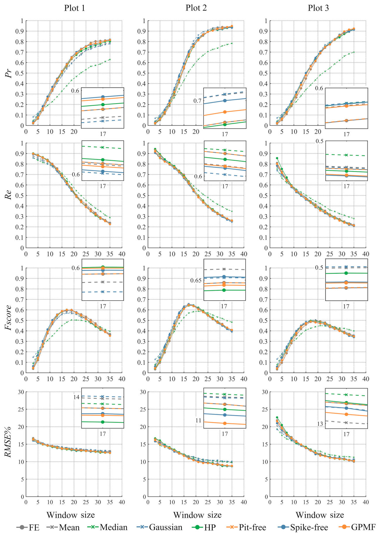
4.1. Sensitivity Analysis

Among the eight CHM generation methods, only the FE method and the HPs methods are parameter-free, and the other six methods require at least one user-defined parameter. These parameters will indeed impact the performance of the methods. To obtain the optimal result of each method and enable a fair comparison, a sensitivity analysis of the parameters was carried out using simulated point clouds with pits of different proportions.

For the global filtering method, mean, medium and Gaussian filtering were performed on CHM_FE with 3 × 3, 5 × 5 and 7 × 7 window sizes, respectively. The results of the comparison of the CHM_Reference against filtered CHMs are shown in Supplementary S1 in the Supplementary Materials, Table S1. The results showed that the median filter and Gaussian filter have the highest accuracies in the 5 × 5 window size, while the mean filter has the highest accuracy in the 3 × 3 window size. The accuracies of the mean filter and median filter were not affected by the proportion of pits or the geometric shape (cone or hemisphere). For a hemisphere with 10% pits, a smaller window is more suitable for Gaussian filtering, and large pits use a large window for Gaussian filtering with higher accuracy.

A user-defined threshold of the pit-free method was controlled from 1% to 30%. The results showed that the accuracy of CHM_pit-free was progressively increased by gradually increasing the threshold (starting from 1 at 5% intervals) (Supplementary S1 in the Supplementary Materials, Table S2). The threshold corresponding to a small proportion of pits reached the optimal solution earlier than the large proportion of pits. When the threshold was 20%, the accuracy reached the highest and remained unchanged.

For the spike-free method, the “freeze distance” and the “insertion buffer” constrained the construction of the TIN. When the freeze distance is increasing, filtered pits also increase, and when the insertion buffer is increased, the constraints loosen. We tested the two parameters through the control variables, and the results showed that although the accuracy was nearly the highest when the freezing distance and the insertion buffer were 0.3 and 0.3 (Supplementary S1 in the Supplementary Materials, Table S3), the visual effect of CHM_Spike-free was the best when the freezing distance and the insertion buffer were 0.4 and 0.5, respectively (Supplementary S1 in the Supplementary Materials, Figure S1).

As the core parameter of the GPMF method, an SI was used to express the depression degree between a point and its neighbourhoods. Here, we adjusted the SI from 0 to 10 with a step of 1 to test the changes in RMSE between the CHM_Reference and the CHM_GPMF. The results showed that the accuracy of the cone gradually decreased from SI = 4, while that of the hemispherical sphere first increased and then decreased with increasing SI (Supplementary S1 in the Supplementary Materials, Table S4). Since the accuracy difference between SI = 3 and 4 was only one in ten thousand, we chose 4 as the optimal parameter of SI.

The comparison of the accuracy of CHMs generated by various methods with optimal parameters and reference CHMs with different proportions of pits is shown in

Table 1. The RMSE (m) of the comparison of CHM_Reference against processed CHMs.

	Proportion of Pits	FE	Mean	Median	Gaussian	HP	Pit-Free	Spike-Free	GPMF
Cone	10%	0.6624	0.4681	0.2547	0.4503	0.4320	0.2195	0.1613	0.0952
	20%	0.9114	0.6601	0.4087	0.6425	0.5461	0.3896	0.1602	0.1096
	30%	1.0808	0.8103	0.5732	0.7935	0.6143	0.5254	0.1648	0.1161
	40%	1.2115	0.9336	0.7214	0.9178	0.6521	0.6437	0.1737	0.1283
	50%	1.3074	1.0294	0.8360	1.0146	0.6656	0.7355	0.1707	0.1337
	60%	1.3933	1.1202	0.9507	1.1061	0.6808	0.8271	0.1707	0.1370
Hemisphere	10%	0.6350	0.4520	0.2421	0.4339	0.4338	0.2124	0.1481	0.0975
	20%	0.8789	0.6277	0.3715	0.6093	0.5497	0.3563	0.1554	0.1090
	30%	1.0392	0.7683	0.5218	0.7511	0.6013	0.4817	0.1579	0.1149
	40%	1.1699	0.8897	0.6578	0.8732	0.6429	0.5956	0.1605	0.1220
	50%	1.2721	0.9901	0.7803	0.9747	0.6721	0.6920	0.1660	0.1311
	60%	1.3612	1.0803	0.8928	1.0656	0.6897	0.7805	0.1659	0.1351

. Notably, the accuracy of all methods decreases with the increase in the proportion of pits. The trend of different methods in different proportions of pits is consistent, which indicates that the data quality has no significant influence on the performance of different methods. Overall, the GPMF method had the lowest RMSE among all the methods, and the spike-free method was the second lowest. The FE method was undoubtedly the worst. The optimal parameters of these methods were used for subsequent applications.

4.2. Comparison of Simulated CHMs

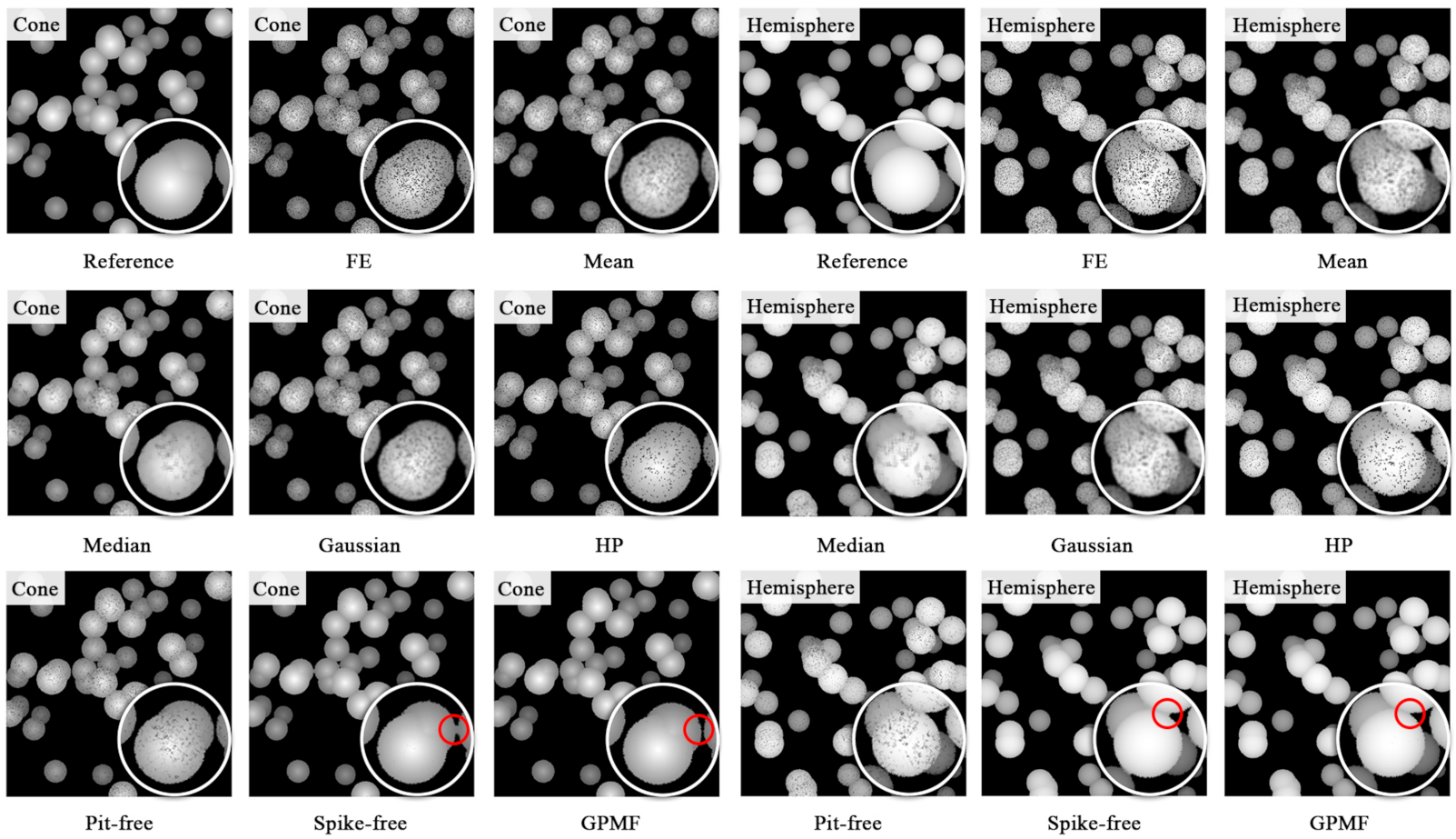
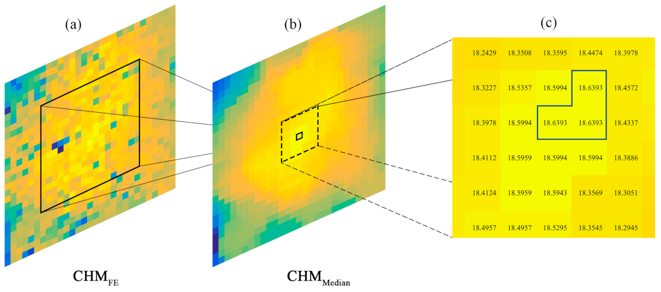
4.2.1. Visual Performance

Taking the data with 20% pits as an example, the 0.1 m resolution CHMs generated by the simulated surface points and the eight processing methods are shown in Figure 4. A visual comparison of these CHMs was implemented. In general, CHM_FE has the largest number of randomly distributed dark pixels, while other CHMs have different degrees of pit-filling. Among them, the visual performance of CHM_Spike-free and CHM_GPMF are closest to that of CHM_Reference. The smooth filtered CHM (CHM_Mean, CHM_Median and CHM_Maussian) made the image blurry, and the pits did not disappear. The performance of CHM_HP and CHM_Pit-free were also not satisfactory. The small pits in the CHM_Pit-free sample were removed, but clustered pits still occurred. A further comparison of CHM_Spike-free and CHM_GPMF found that CHM_GPMF has a clearer crown edge, and the connection between adjacent canopies is also better processed, while there is adhesion at the adjacent canopy of CHM_Spike-free (see the red circle in Figure 4). In addition, we found that there are many pits in the overlapping crown of the hemispherical model, and only the spike-free and GPMF methods can filter these pits well.

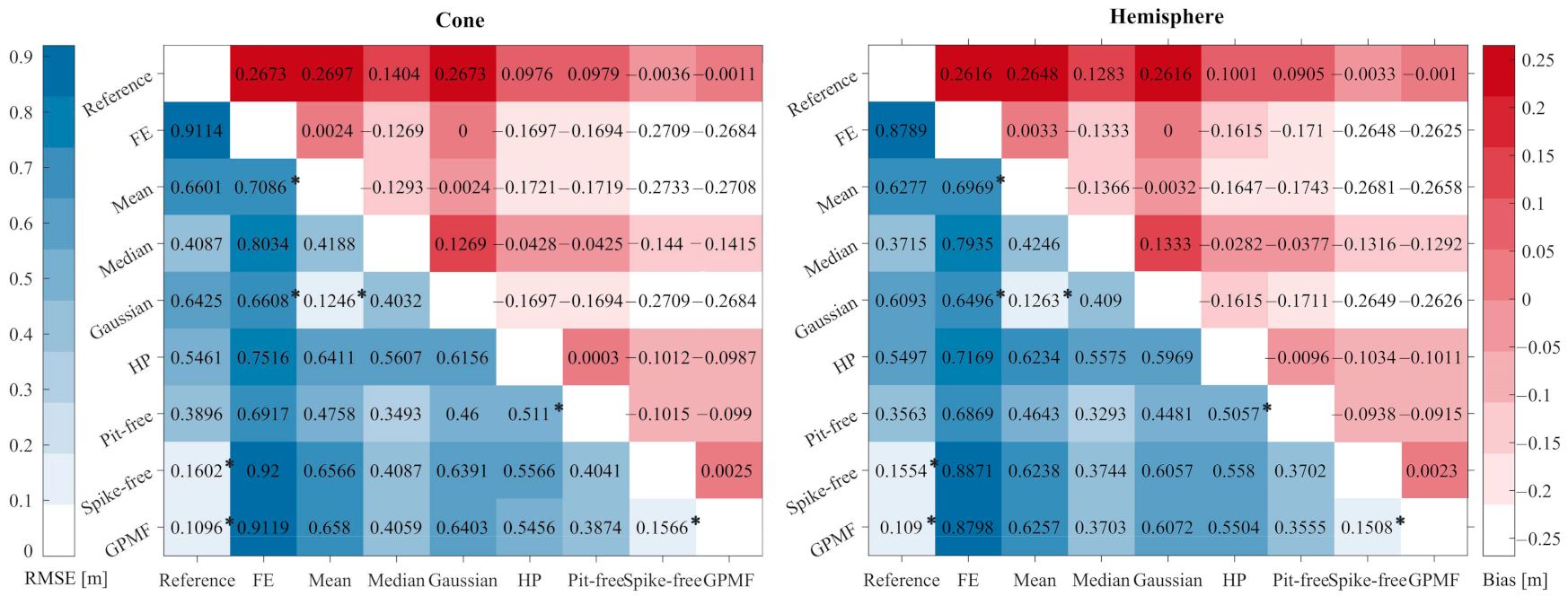
4.2.2. Quantitative Analysis

A further quantitative comparison of the differences between these methods is shown in Figure 5. The results indicated that only CHM_Spike-free and CHM_GPMF have no significant difference from CHM_Reference (RMSEs are 0.1602 m and 0.1096 m, and RMSE% values are 1.86% and 1.27% of cone, respectively). The difference between CHM_Reference and CHM_FE was the largest (RMSE = 0.9114 m, RMSE% = 10.6%), which was approximately 9% lower than CHM_Spike-free and CHM_GPMF. There was no significant difference between the mean heights of CHM_Mean and CHM_Gaussian and that of CHM_FE. Additionally, the mean heights of CHM_HP and CHM_Pit-free showed no significant difference. In terms of Bias, we found that the spike-free and GPMF methods slightly overestimated the crown surface height, and the other six methods underestimated it. The results also showed that the median filtering method has the highest accuracy among the three smooth filtering methods. The application of the eight processing methods was not different in the cone and hemisphere.

4.3. Comparison of UAVLS-Derived CHMs

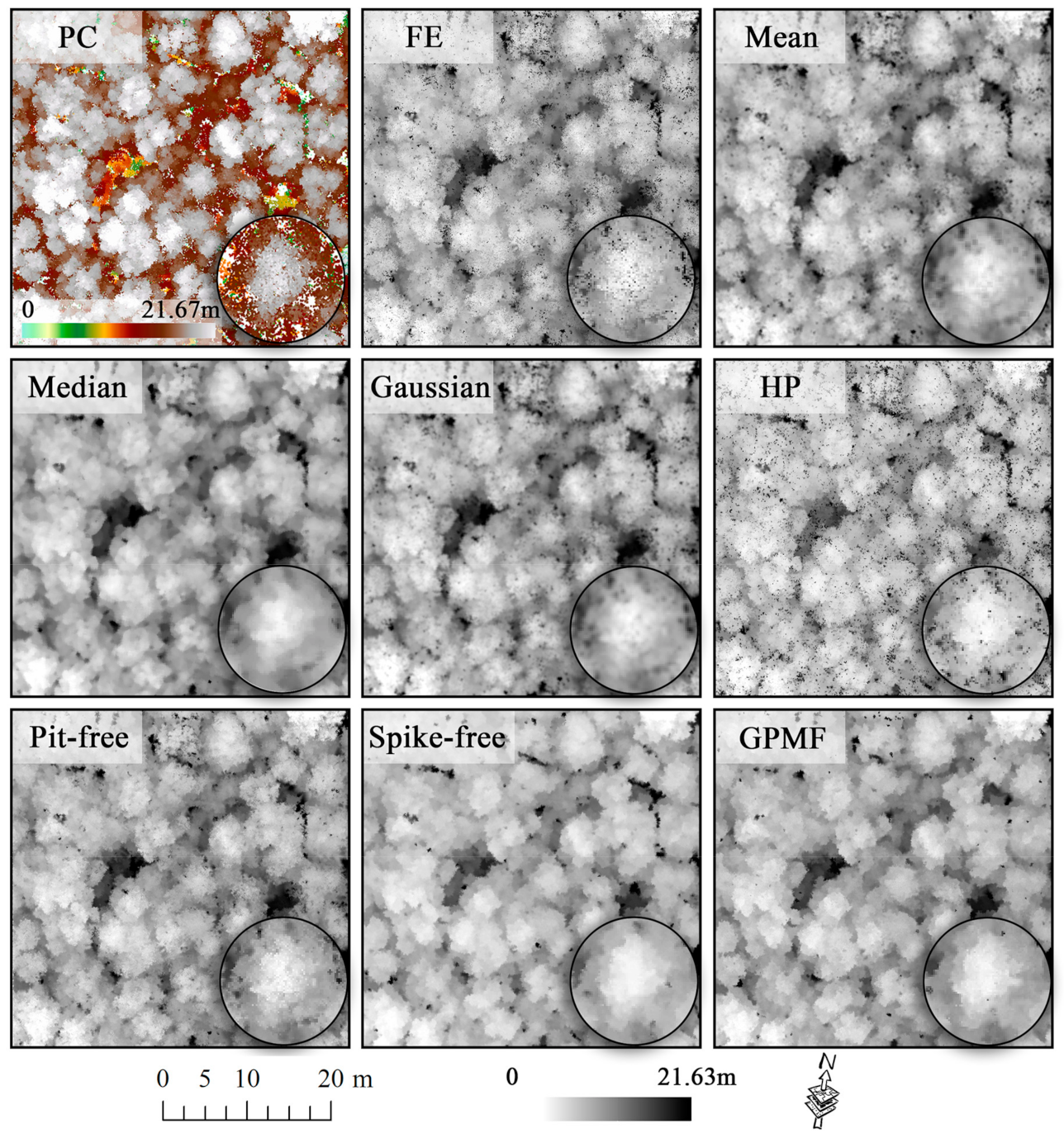
4.3.1. Visual Performance

For clarity, the CHMs of four subplot sizes in Plot 3 were selected as examples and are shown in Figure 6. The median filter method eliminates almost all the pits, but the image is excessively smooth and the crown shape is blurred. Although the HP method makes the crown clearly visible, it produces more clumps and black pits than the FE method. The Gaussian filter is more blurred than the mean filter, and at the same time, it does not improve the pit problem. Overall, the spike-free and GPMF methods achieved the best visual performances of all the methods, followed by the pit-free method.

Figure 7 provides an example of a 0.1 m wide canopy profile highlighting the difference between laser points and the CHMs generated by eight methods. The FE points are not only distributed on the surface of the canopy but also distributed in the canopy or even on the ground, which directly leads to CHM_FE with many depressions. Among all the methods, we first noticed the HP profile because it produced sharper and deeper peaks than FE. The pit-free method only fills in the local pits, and the other parts are consistent with the FE profile. In general, the CHM_Spike-free and CHM_GPMF were closest to the surface of the point cloud, while the smoothed CHMs were seriously underestimated. Notably, the GPMF pulled up some valleys between the two crowns, but this phenomenon is likely due to the influence of the Y-axis neighbourhood and not just the X-axis neighbourhood; thus, the GPMF accuracy needs to be further evaluated.

4.3.2. Quantitative Analysis

Table 2. Differences across all the CHMs generated by the UAVLS point cloud. The lower left corner of the matrix is the RMSE (m), and the upper right corner of the matrix is the Bias (m).

	Method	FE	Mean	Median	Gaussian	HP	Pit-Free	Spike-Free	GPMF
Plot1	FE	-	0.0000	−0.2798	0.0000	0.0105	−0.3264	−0.6280	−0.6273
	Mean	1.1291 *	-	−0.2799	0.0000	0.0104	−0.3264	−0.6280	−0.6273
	Median	1.4089	0.7120	-	0.2798	0.2903	−0.0466	−0.3482	−0.3475
	Gaussian	1.0650 *	0.1650 *	0.6608	-	0.0105	−0.3264	−0.6280	−0.6273
	HP	1.8070	1.7031	1.7973	1.6789	-	−0.3369	−0.6385	−0.6378
	Pit-free	1.1468	0.6940	0.6323	0.6647	1.6962	-	−0.3016	−0.3009
	Spike-free	1.7900	1.3391	1.0497	1.3102	1.8219	1.0789	-	0.0007
	GPMF	1.7425	1.2841	0.9677	1.2494	1.9408	1.0216	0.9356 *	-
Plot2	FE	-	0.0000	−0.3070	0.0000	0.1037	−0.4020	−0.8574	−0.9324
	Mean	1.3112 *	-	−0.3069	0.0000	0.1038	−0.4019	−0.8574	−0.9323
	Median	1.6450	0.8114	-	0.3070	0.4107	−0.0950	−0.5505	−0.6254
	Gaussian	1.2459 *	0.1938 *	0.7492	-	0.1037	−0.4020	−0.8574	−0.9324
	HP	2.1693	2.0782	2.2074	2.0526	-	−0.5057	−0.9612	−1.0361
	Pit-free	1.2624	0.8422	0.8646	0.8174	2.0750	-	−0.4555	−0.5304
	Spike-free	2.2619	1.7930	1.5187	1.7636	2.2716	1.5274	-	−0.0749
	GPMF	2.2495	1.7740	1.4720	1.7382	2.4812	1.5107	1.3075	-
Plot3	FE	-	-0.0001	−0.2580	0.0000	0.1854	−0.3489	−0.7381	−0.7485
	Mean	1.1884 *	-	−0.2580	0.0001	0.1854	−0.3488	−0.7380	−0.7484
	Median	1.4536	0.7054	-	0.2580	0.4434	−0.0909	−0.4801	−0.4905
	Gaussian	1.1215 *	0.1748 *	0.6497	-	0.1854	−0.3489	−0.7381	−0.7485
	HP	2.4499	2.3126	2.3662	2.2942	-	−0.5343	−0.9234	−0.9339
	Pit-free	1.1670	0.7407	0.7105	0.7126	2.3038	-	−0.3892	−0.3996
	Spike-free	2.1171	1.7104	1.4729	1.6850	2.2822	1.4845	-	−0.0104
	GPMF	2.0048	1.5767	1.3130	1.5450	2.4923	1.3449	1.2313	-

* t-test shows no significant difference.

shows the RMSE and Bias values between the eight CHM generation methods. The cross-comparison results showed that there was no significant difference between CHM_Mean and CHM_Gaussian. The mean heights of the CHM_Spike-free and CHM_GPMF were not significantly different in broad-leaved forests. The difference between FE and other CHMs was higher than 1 m, of which the largest was HP (2.4499 m of Plot 3). The Bias between mean filtering and median filtering and FE is 0, indicating that these two filtering methods have not changed the average height of the CHM. Among the eight CHMs, CHM_Spike-free had the highest average height in broadleaf forests, while CHM_GPMF had the highest average height in coniferous and mixed forests. The average value of CHM_HP is the lowest, which may be because too many extremely deep pits reduce the average HP based on the abovementioned canopy profile (Figure 7). In coniferous forests, the difference between the eight methods was the largest.

When the reference surface points were introduced to evaluate the performance of the eight methods, the results are shown in

Table 3. Verification results of different CHMs and reference canopy surface points.

	Method	Peak			Valley			Overall
		R2	Bias (m)	RMSE (m)	R2	Bias (m)	RMSE (m)	R2	Bias (m)	RMSE (m)
Plot1	FE	0.82	0.5703	0.9928	0.93	0.3427	0.6356	0.88	0.4543	0.8301
	Mean	0.86	0.8258	1.0654	0.84	0.8002	1.1172	0.86	0.8128	1.0921
	Median	0.91	0.7139	0.8832	0.98	0.3715	0.4494	0.95	0.5393	0.6967
	Gaussian	0.86	0.8668	1.0908	0.89	0.7329	0.9747	0.89	0.7986	1.0332
	HP	0.98	0.1585	0.3037	0.91	0.2112	0.6318	0.94	0.1854	0.4987
	Pit-free	0.95	0.4140	0.5773	0.95	0.2827	0.5053	0.95	0.3470	0.5418
	Spike-free	0.99	0.1801	0.2766	1.00	0.0829	0.1315	0.99	0.1306	0.2152
	GPMF	0.99	0.2186	0.2998	0.98	0.1453	0.3269	0.98	0.1812	0.3139
Plot2	FE	0.52	1.0193	2.1159	0.70	0.7952	1.6607	0.67	0.9058	1.8990
	Mean	0.72	1.4988	1.8005	0.83	1.1116	1.4945	0.83	1.3026	1.6526
	Median	0.87	1.1726	1.3415	0.88	0.8567	1.2020	0.90	1.0126	1.2727
	Gaussian	0.75	1.4979	1.7743	0.85	1.1134	1.4524	0.84	1.3031	1.6192
	HP	0.90	0.3282	0.6553	0.88	0.4779	0.9246	0.92	0.4041	0.8031
	Pit-free	0.91	0.5997	0.8012	0.87	0.5869	1.0497	0.91	0.5932	0.9354
	Spike-free	0.99	0.2139	0.2895	0.97	0.2245	0.4448	0.98	0.2193	0.3763
	GPMF	0.99	0.3037	0.3710	0.95	0.2375	0.5728	0.97	0.2702	0.4839
Plot3	FE	0.53	0.5059	1.6823	0.74	0.4354	1.5109	0.70	0.9414	1.5983
	Mean	0.69	0.6556	1.5872	0.82	0.6037	1.5287	0.81	1.2594	1.5580
	Median	0.80	0.5384	1.2751	0.89	0.4986	1.2282	0.89	1.0370	1.2517
	Gaussian	0.71	0.6597	1.5690	0.83	0.6127	1.5212	0.83	1.2724	1.5451
	HP	0.94	0.1181	0.4526	0.77	0.2761	1.1566	0.86	0.3942	0.8804
	Pit-free	0.80	0.3717	1.0157	0.89	0.3299	0.9703	0.89	0.7016	0.9931
	Spike-free	0.97	0.1188	0.3450	0.98	0.1066	0.3785	0.98	0.2255	0.3622
	GPMF	0.97	0.1521	0.4043	0.94	0.1733	0.6063	0.96	0.3254	0.5160
Avg.	FE	0.62	0.6985	1.5970	0.79	0.5244	1.2691	0.75	0.7672	1.4425
	Mean	0.76	0.9934	1.4844	0.83	0.8385	1.3801	0.83	1.1249	1.4342
	Median	0.86	0.8083	1.1666	0.92	0.5756	0.9599	0.91	0.8630	1.0737
	Gaussian	0.77	1.0081	1.4780	0.86	0.8197	1.3161	0.85	1.1247	1.3992
	HP	0.94	0.2016	0.4705	0.85	0.3217	0.9043	0.91	0.3279	0.7274
	Pit-free	0.89	0.4618	0.7981	0.90	0.3998	0.8418	0.92	0.5473	0.8234
	Spike-free	0.98	0.1709	0.3037	0.98	0.1380	0.3183	0.98	0.1918	0.3179
	GPMF	0.98	0.2248	0.3584	0.96	0.1854	0.5020	0.97	0.2589	0.4379

. Overall, the spike-free method showed the best performance in terms of overall accuracy, and the GPMF was suboptimal. The HP method showed good performance in the peak canopy but poor performance in the valley. In contrast, the median performed well in the valley of the canopy but poorly in the peak. The mean filter performed the worst not only in the peak of the canopy but also in the valley. Compared with the canopy valley, the accuracy loss of the canopy peak was the main disadvantage of FE. The spike-free and GPMF methods have a strong ability to explain canopy surface height variation (R² close to 1, and RMSE% less than 3%). Overall, all the methods underestimated the reference surface (Bias > 0), of which the mean filter method underestimated the surface the most (Bias% = 7.73%) and the spike-free method underestimated the surface the least (Bias% = 1.32%).

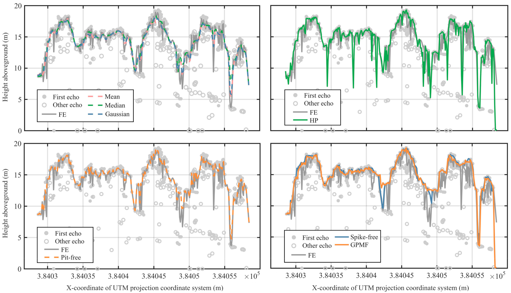
4.3.3. Individual Tree Application Evaluation

The local maxima algorithm was applied to all the processed CHMs. Figure 8 illustrates the accuracy of ITD and tree height estimation plotted against window size (WS) of the local maxima algorithm. Overall, with the increase in WS, the Pr of all the methods increases, the Re and RMSE% decrease and F_score presents a “mountain” shape, which first increases to a maximum value and then decreases. That is, the commission error always increases with increasing WS, while the omission error is the opposite. When the commission and omission errors become balanced, the overall accuracy reaches the maximum value. The accuracy of tree height estimation decreased with increasing WS.

Further analysis showed that the sensitivity of different CHMs to the LM of different WSs was slightly different. In terms of the accuracy of ITD, the median method was the main outlier in the eight methods. Basically, the median filtering CHM performed best in controlling omission errors, but mass commission errors led to the lowest Pr and F_score values. In addition, almost all methods achieved the highest overall accuracy (F_score) when WS was 17 × 17 (1.7 m × 1.7 m). Therefore, the small window in Figure 8 is partially enlarged when WS is equal to 17. The dotted line and the solid line represent four post-processing methods and four pre-processing methods, respectively. As there is little difference between these methods, we evaluated them by 50% of the rankings. Specifically, for broadleaf forest, the HP, GPMF and spike-free methods were in the top 50% due to their excellent performances in controlling the commission error. For coniferous and mixed forests, the mean and Gaussian filter showed remarkable performances. For the spike-free method, even if there is an enormous omission error, the extremely high commission error control gives it a high overall accuracy in each stand type. In addition, we found that the post-processing method (mean, median, Gaussian and pit-free method) had a small omission error (Re is usually high), which may benefit from excessive detection.

In terms of tree height estimation (RMSE%), we found that coniferous forest has the highest accuracy compared with broad-leaved forest and mixed forest, and the WS has the greatest influence on the estimation accuracy of mixed forest. The GPMF and spike-free method always achieved high accuracy regardless of the forest stand. The HP method performed well in broadleaf and coniferous forests, and the mean filter performed well in mixed forests. In coniferous forests, when WS gradually increases, the tree height estimation accuracies of the three smooth filtering methods become increasingly lower, and the difference compared with other methods increases significantly. The accuracy of the median filter method was significantly lower than that of the other methods in mixed forests. In addition, the difference from other methods was not obvious.

5. Discussion

In recent years, an increasing number of studies have directly used UAVLS as a measurement tool due to the high-density point cloud data, which requires data processing to minimize the loss of accuracy. As one of the inherent problems in the processing of LiDAR data, pits will seriously affect the quality of the CHM [9]. Although many studies focus on pit-filling of the CHMs, most of these algorithms were developed and applied to low-density ALS (0.7–8 pt/m²) to generate CHMs from 0.2 m to 0.5 m [7,9,11,12,25,26,27]. In the present study, we evaluated the performances of several pit-filling methods for generating 0.1 m resolution CHMs by using both high-density simulated data and UAVLS data. A comprehensive visual performance, quantitative analysis and application evaluation framework was used to compare these CHMs.

Compared with real laser scanning data, artificially constructed simulated PCs can define the exact canopy surface to intuitively and quantitatively compare the effects of different methods [11,26]. In terms of the simulated data results, we obtained a clear ranking of the advantages and disadvantages in the eight methods (the order is GPMF, spike-free, pit-free, median, HP, Gaussian, and mean). In contrast, there are many uncertainties in the real UAV point cloud, which makes the results more complicated. In particular, the UAVLS data for this study were collected from natural secondary forests with diverse tree species, high stand density and complex forest layers. The sources of data pits may vary, and it is difficult to find a true canopy surface as a reference to verify different CHMs. Previous studies have used different techniques to assess the accuracy of these pit-filling algorithms. Ben-Arie et al. [10] visually compared the efficacy of the pit-filling algorithm through CHM and its X-axis profile. Khosravipour et al. [4,17] evaluated the spike-free method using the accuracy of ITD. Hao et al. [27] first segmented individual trees and then selected convex hull vertices above the maximum crown diameter of each individual tree as reference surface points. Mielcarek et al. [7] tested and evaluated five CHM generation methods by the accuracy of tree height estimation. Chen et al. [11] and Zhang et al. [26] evaluated the accuracy of only plot-level maximum tree height estimation. By comparison, the evaluation framework we used can comprehensively and systematically compare the effects of different methods.

Regarding the results of the UAVLS-derived CHM evaluation, the GPMF and spike-free method showed optimal visual performances, similar to the simulated data, and they produced few pits while preserving details of the crown. The verification of canopy surface points indicated that the spike-free method performed slightly better than the GPMF method. The accuracy of ITD for broadleaf forest and tree height estimation of the GPMF method was slightly better than that of the spike-free method. For the FE method, since the first return not only exists on the canopy surface but is also distributed inside the canopy and on the surface (Figure 7), it produced the most data pits among all methods. This confirmation is consistent with the results from [9,10,28]. For the global filtering method, the accuracy of the median filter CHM construction was better than that of mean and Gaussian, but the accuracy of the median filter CHM application showed outliers. Further analysis found that the median filter produced many consecutive equal pixel values, which led to multiple continuous treetops in the LM filter and significantly increased the commission error (shown in Figure 9). The canopy height was significantly underestimated, and this method produced a mass commission error [27]. For the pit-free method, the ITD and tree height estimation results are almost consistent with those of the FE method because it only fills the filtered pits based on FE [7,27]. Thus, although the post-processing methods based on the original CHM have eliminated partial pits in the visual effect, they show limited improvement in the quality of the CHM and are even lower than the original CHM [27]. For the HP method, although it eliminates some small pits, this method produces deeper pits compared with the FE method, which will greatly reduce the average height. However, a small number of deep pits do not affect LM detection, so it is not restricted to individual tree applications. Hao et al. [27] claimed that the HP method is sensitive to the density of the point cloud; when the pixel is too large, the details of the crown are missed. Leckie et al. [12] set the grid pixel size at 25 cm according to the average point spacing. Our average point spacing was between 0.06 m and 0.08 m, so a 0.1 m resolution was appropriate.

According to the description of Shamsoddini et al. [9], a robust pit-filling algorithm needs to satisfy the following criteria: identify pits using an adaptive threshold, perform oriented detection of pits without changing the maximum value, fill the pits with suitable values to represent the crown shape as closely as possible and preserve canopy gaps. Considering the driving parameters of the algorithm, the GPMF method and pit-free algorithm are parameter-driven algorithms, the spike-free method has two user-defined parameters, the filter method requires the WS be set, and the FE and HP methods have no parameters. The spike-free and GPMF differ fundamentally from the others; they used all laser returns to generate CHMs while improving the potential pits. Using all returns avoids the loss of crown information and eliminates some errors caused by using only the first return [7,45]. The difference between them is that the spike-free algorithm prevents spike formation during TIN construction [17], while GPMF excludes non-surface points from all returns in a progressive filtering process [27]. GPMF is similar to ground point filtering [11]; it screens surface points from laser scanning data and can be used for other canopy surface studies. Compared with other methods, the spike-free method was developed based on high-density PCs, which is beneficial to the application of this method in high-resolution CHM generation. Although the CHM filtering method underestimates the canopy height, it is simple to process and could prove useful for other applications. For example, Shamsoddini et al. [9] pointed out that CHM filtering combined with linear regression has an excellent performance in estimating tree height. The error of the post-processing method mainly comes from the canopy peak, and the error of the pre-processing method mainly comes from the valley (Table 3), which proves that the pre-processing method can orient the detection of pits without changing the maximum value.

By comparing the results of different forest types, the average height difference in the CHM generated by different methods in coniferous forests is the largest (Figure 5 and Table 2), indicating that the impact of pits is worth consideration when generating a CHM of coniferous forests. The FE and filter CHM severely underestimated the heights of coniferous forests, especially for the peak canopy (Table 3), because coniferous crowns are conical and easy to wear during filtration. The accuracy difference between the GPMF method and spike-free algorithm mixed forests is larger than that of the other forest types, which indicates that the adaptability of the GPMF method in complex forests is not as good as that in spike-free forests. Regarding the detection of individual trees, coniferous forests have higher overall accuracies than broad-leaved forests and mixed forests because of their lower commission errors (Figure 8). Likewise, the tree height estimation accuracy of coniferous forest was the highest among the three forest types when the detection WS was the same. The accuracies of ITD and tree height estimation of mixed forest were the lowest.

This study demonstrated that the effect of the pit-filling method on individual tree applications of high-resolution CHMs is small. The outliers of the median filter in broad-leaved forest, coniferous forest and mixed forest were 12%, 9% and 8%, respectively. The differences from other methods for different forest types are very small (the difference of F_score was 1–3%), while the accuracies of different methods for estimating tree height in any forest was less than 0.1%. This result indicated that the effect of data pits on individual tree applications (ITD and tree height estimation) is not significant when using a high-resolution CHM. Perhaps with the decrease in resolution, the difference will be more obvious. For example, the results of Mielcarek et al. [7] showed that the difference in tree height estimation accuracy between spike-free and Gaussian filters is 3.29% when using a 0.5 m resolution CHM. Hao et al. [27] showed that the difference in the overall accuracy of ITD between GPMF and FE is 17.43%. The results of Khosravipour et al. [4] show that the accuracy difference between the pit-free CHM developed by Khosravipour et al. [4] and the Gaussian smoothed CHM is 3.6% when using a 0.15 m resolution CHM, while the difference is 32% when using a 0.5 m resolution CHM.

This study aims to compare and evaluate the performances of different pit-filling methods to generate high-resolution CHMs. To reduce the uncertainty of complex parameter selection in the ITD algorithm, a single parameter and commonly used local maxima detection method are used. Although there is little difference in the application of individual trees, notably, CHMs without artefacts are more useful and reliable, with better reproductions of crown shapes [7]. Other CHM applications should be further evaluated, such as crown delineation and other tree metric estimations, and more data set from complicated natural forests would be recommended to take into account for evaluating the effectiveness of the framework on the diverse tree species, high stand density, and complex forest layers. Notably, this study area is a natural secondary forest with high-density stems, and it is difficult to measure individual tree position and height. Due to many uncertainties in field measurements [7], many studies suggest that LiDAR be directly used as a measurement tool [46,47]. Based on the topography of the study area (7° to 11°), there is no significant difference between the CHM generated by normalized PCs and the CHM obtained by the DSM minus DEM, regardless of the method used.

6. Conclusions

The high sampling density near-ground UAVLS system can extract fine forest canopy structures. Quantifying the accuracy of high-resolution CHM construction derived from UAVLS is an important precursor to the use of UAVLS data to obtain other forest parameters. This study compared and evaluated several CHM generation methods from multiple aspects. The results demonstrated that different processing methods can affect the quality of the CHMs generated by high-resolution UAVLS data. The GPMF [27] and spike-free [17] methods have excellent performance in generating CHMs; they effectively remove data pits and preserve crown details, while minimizing the loss of canopy height under complex stand conditions. Using the first echo of laser scanning will produce massive amounts of data noise and result in the incorrect expression of the canopy surface. Although the global filtering method (mean, median and Gaussian filter) of the CHM decreases the noise visually, it significantly reduces the canopy surface height. A median filter is not suitable for individual tree applications based on LM detection when using a high-resolution CHM. The pit-free method [10] detects and fills pits locally in the original CHM, and it can improve limited accuracy, similar to other post-processing methods. The HP interpolation method [12] has a good performance in the generation of high-resolution CHMs, but a small number of deep points are introduced. In high-density and complex forests, the suppressed tree crown is also an important source of CHM pits. Compared with broad-leaved and mixed forests, coniferous forests are more sensitive to data pits, so selection of the CHM generation method should be considered. Although these high-resolution CHM generation methods show little difference in the application of ITD and tree height estimation, a CHM without noise is also valuable. This study provides a comprehensive reference for CHM generation using high-resolution LiDAR data and demonstrates the potential of UAVLS as a forest measurement tool in obtaining forest inventories.

References

1. Hyyppä, J.; Hyyppä, H.; Leckie, D.; Gougeon, F.; Yu, X.; Maltamo, M. Review of methods of small-footprint airborne laser scanning for extracting forest inventory data in boreal forests. Int. J. Remote Sens. 2008, 29, 1339–1366. [Google Scholar] [CrossRef]
2. Lim, K.; Treitz, P.; Wulder, M.; St-Onge, B.; Flood, M. LiDAR remote sensing of forest structure. Prog. Phys. Geogr. 2003, 27, 88–106. [Google Scholar] [CrossRef] [Green Version]
3. Popescu, S.C.; Wynne, R.H.; Nelson, R.F. Estimating plot-level tree heights with lidar: Local filtering with a canopy-height based variable window size. Comput. Electron. Agric. 2002, 37, 71–95. [Google Scholar] [CrossRef]
4. Khosravipour, A.; Skidmore, A.K.; Isenburg, M.; Wang, T.; Hussin, Y.A. Generating Pit-free Canopy Height Models from Airborne Lidar. Photogramm. Eng. Remote Sens. 2014, 80, 863–872. [Google Scholar] [CrossRef]
5. Zhang, C.; Zhou, Y.; Qiu, F. Individual Tree Segmentation from LiDAR Point Clouds for Urban Forest Inventory. Remote Sens. 2015, 7, 7892–7913. [Google Scholar] [CrossRef] [Green Version]
6. Zhen, Z.; Quackenbush, L.; Zhang, L. Trends in Automatic Individual Tree Crown Detection and Delineation—Evolution of LiDAR Data. Remote Sens. 2016, 8, 333. [Google Scholar] [CrossRef] [Green Version]
7. Mielcarek, M.; Stereńczak, K.; Khosravipour, A. Testing and evaluating different LiDAR-derived canopy height model generation methods for tree height estimation. Int. J. Appl. Earth Obs. Geoinf. 2018, 71, 132–143. [Google Scholar] [CrossRef]
8. Yao, W.; Krzystek, P.; Heurich, M. Tree species classification and estimation of stem volume and DBH based on single tree extraction by exploiting airborne full-waveform LiDAR data. Remote Sens. Environ. 2012, 123, 368–380. [Google Scholar] [CrossRef]
9. Shamsoddini, A.; Turner, R.; Trinder, J.C. Improving lidar-based forest structure mapping with crown-level pit removal. J. Spat. Sci. 2013, 58, 29–51. [Google Scholar] [CrossRef]
10. Ben-Arie, J.R.; Hay, G.J.; Powers, R.P.; Castilla, G.; St-Onge, B. Development of a pit filling algorithm for LiDAR canopy height models. Comput. Geosci. 2009, 35, 1940–1949. [Google Scholar] [CrossRef]
11. Chen, C.; Wang, Y.; Li, Y.; Yue, T.; Wang, X. Robust and Parameter-Free Algorithm for Constructing Pit-Free Canopy Height Models. ISPRS Int. J. Geo Inf. 2017, 6, 219. [Google Scholar] [CrossRef] [Green Version]
12. Leckie, D.; Gougeon, F.; Hill, D.; Quinn, R.; Armstrong, L.; Shreenan, R. Combined high-density lidar and multispectral imagery for individual tree crown analysis. Can. J. Remote Sens. 2003, 29, 633–649. [Google Scholar] [CrossRef]
13. Persson, Å.; Holmgren, J.; Söderman, U. Detecting and measuring individual trees using an airborne laser scanner. Photogramm. Eng. Remote Sens. 2002, 68, 925–932. [Google Scholar]
14. Puttonen, E.; Litkey, P.; Hyyppä, J. Individual Tree Species Classification by Illuminated—Shaded Area Separation. Remote Sens. 2010, 2, 19–35. [Google Scholar] [CrossRef] [Green Version]
15. Vosselman, G. Analysis of planimetric accuracy of airborne laser scanningsurveys. ISPRS Arch. 2008, 37, 99–104. [Google Scholar]
16. Goulden, T.; Hopkinson, C. The Forward Propagation of Integrated System Component Errors within Airborne Lidar Data. Photogramm. Eng. Remote Sens. 2010, 76, 589–601. [Google Scholar] [CrossRef]
17. Khosravipour, A.; Skidmore, A.K.; Isenburg, M. Generating spike-free digital surface models using LiDAR raw point clouds: A new approach for forestry applications. Int. J. Appl. Earth Obs. Geoinf. 2016, 52, 104–114. [Google Scholar] [CrossRef]
18. Reitberger, J.; Schnörr, C.; Krzystek, P.; Stilla, U. 3D segmentation of single trees exploiting full waveform LIDAR data. ISPRS J. Photogramm. Remote 2009, 64, 561–574. [Google Scholar] [CrossRef]
19. Gaveau, D.; Hill, R.A. Quantifying canopy height underestimation by laser pulse penetration in small-footprint airborne laser scanning data. Can. J. Remote Sens. 2003, 29, 650–657. [Google Scholar] [CrossRef]
20. Reuter, H.I.; Hengl, T.; Gessler, P.; Soille, P. Chapter 4 Preparation of DEMs for Geomorphometric Analysis. Dev. Soil Sci. 2009, 33, 87–120. [Google Scholar]
21. Priestnall, G.; Jaafar, J.; Duncan, A. Extracting urban features from LiDAR digital surface models. Comput. Environ. Urban Syst. 2000, 24, 65–78. [Google Scholar] [CrossRef]
22. Macmillan, R.A.; Martin, T.C.; Earle, T.J.; Mcnabb, D.H. Automated analysis and classification of landforms using high-resolution digital elevation data: Applications and issues. Can. J. Remote Sens. 2003, 29, 592–606. [Google Scholar] [CrossRef]
23. Koch, B.; Heyder, U.; Weinacker, H. Detection of Individual Tree Crowns in Airborne Lidar Data. Photogramm. Eng. Remote Sens. 2006, 72, 357–363. [Google Scholar] [CrossRef] [Green Version]
24. Zhao, D.; Pang, Y.; Li, Z.; Sun, G. Filling invalid values in a lidar-derived canopy height model with morphological crown control. Int. J. Remote Sens. 2013, 34, 4636–4654. [Google Scholar] [CrossRef]
25. Liu, H.; Dong, P. A new method for generating canopy height models from discrete-return LiDAR point clouds. Remote Sens. Lett. 2014, 5, 575–582. [Google Scholar] [CrossRef]
26. Zhang, W.; Cai, S.; Liang, X.; Shao, J.; Hu, R.; Yu, S.; Yan, G. Cloth simulation-based construction of pit-free canopy height models from airborne LiDAR data. For. Ecosyst. 2020, 7. [Google Scholar] [CrossRef] [Green Version]
27. Hao, Y.; Zhen, Z.; Li, F.; Zhao, Y. A graph-based progressive morphological filtering (GPMF) method for generating canopy height models using ALS data. Int. J. Appl. Earth Obs. Geoinf. 2019, 79, 84–96. [Google Scholar] [CrossRef]
28. Hao, Y.; Widagdo, F.R.A.; Liu, X.; Quan, Y.; Dong, L.; Li, F. Individual Tree Diameter Estimation in Small-Scale Forest Inventory Using UAV Laser Scanning. Remote Sens. 2020, 13, 24. [Google Scholar] [CrossRef]
29. Quan, Y.; Li, M.; Zhen, Z.; Hao, Y.; Wang, B. The Feasibility of Modelling the Crown Profile of Larix olgensis Using Unmanned Aerial Vehicle Laser Scanning Data. Sensors 2020, 20, 5555. [Google Scholar] [CrossRef] [PubMed]
30. Jaakkola, A.; Hyyppä, J.; Kukko, A.; Yu, X.; Kaartinen, H.; Lehtomäki, M.; Lin, Y. A low-cost multi-sensoral mobile mapping system and its feasibility for tree measurements. ISPRS J. Photogramm. Remote 2010, 65, 514–522. [Google Scholar] [CrossRef]
31. Liu, Q.; Fu, L.; Chen, Q.; Wang, G.; Luo, P.; Sharma, R.P.; He, P.; Li, M.; Wang, M.; Duan, G. Analysis of the Spatial Differences in Canopy Height Models from UAV LiDAR and Photogrammetry. Remote Sens. 2020, 12, 2884. [Google Scholar] [CrossRef]
32. Wulder, M.; Niemann, K.O.; Goodenough, D.G. Local Maximum Filtering for the Extraction of Tree Locations and Basal Area from High Spatial Resolution Imagery. Remote Sens. Environ. 2000, 73, 103–114. [Google Scholar] [CrossRef]
33. Yin, D.; Wang, L. Individual mangrove tree measurement using UAV-based LiDAR data: Possibilities and challenges. Remote Sens. Environ. 2019, 223, 34–49. [Google Scholar] [CrossRef]
34. Bater, C.W.; Coops, N.C. Evaluating error associated with lidar-derived DEM interpolation. Comput. Geosci. 2009, 35, 289–300. [Google Scholar] [CrossRef]
35. Hu, T.; Sun, X.; Su, Y.; Guan, H.; Sun, Q.; Kelly, M.; Guo, Q. Development and Performance Evaluation of a Very Low-Cost UAV-Lidar System for Forestry Applications. Remote Sens. 2020, 13, 77. [Google Scholar] [CrossRef]
36. Ota, T.; Ogawa, M.; Mizoue, N.; Fukumoto, K.; Yoshida, S. Forest Structure Estimation from a UAV-Based Photogrammetric Point Cloud in Managed Temperate Coniferous Forests. Forests 2017, 8, 343. [Google Scholar] [CrossRef]
37. Jaakkola, A.; Hyyppä, J.; Yu, X.; Kukko, A.; Kaartinen, H.; Liang, X.; Hyyppä, H.; Wang, Y. Autonomous Collection of Forest Field Reference—The Outlook and a First Step with UAV Laser Scanning. Remote Sens. 2017, 9, 785. [Google Scholar] [CrossRef] [Green Version]
38. Dong, P. Characterization of individual tree crowns using three-dimensional shape signatures derived from LiDAR data. Int. J. Remote Sens. 2009, 30, 6621–6628. [Google Scholar] [CrossRef]
39. Axelsson, P. DEM generation from laser scanner data using adaptive TIN models. ISPRS Arch. 2000, 33, 110–117. [Google Scholar]
40. Guo, Q.; Li, W.; Yu, H.; Alvarez, O. Effects of Topographic Variability and Lidar Sampling Density on Several DEM Interpolation Methods. Photogramm. Eng. Remote Sens. 2010, 76, 701–712. [Google Scholar] [CrossRef] [Green Version]
41. Li, W.; Guo, Q.; Jakubowski, M.K.; Kelly, M. A New Method for Segmenting Individual Trees from the Lidar Point Cloud. Photogramm. Eng. Remote Sens. 2012, 78, 75–84. [Google Scholar] [CrossRef] [Green Version]
42. Chen, Q.; Baldocchi, D.; Gong, P.; Kelly, M. Isolating Individual Trees in a Savanna Woodland using Small Footprint LIDAR data. Photogramm. Eng. Remote Sens. 2006, 72, 923–932. [Google Scholar] [CrossRef] [Green Version]
43. Zhen, Z.; Quackenbush, L.J.; Stehman, S.V.; Zhang, L. Agent-based region growing for individual tree crown delineation from airborne laser scanning (ALS) data. Int. J. Remote Sens. 2015, 36, 1965–1993. [Google Scholar] [CrossRef]
44. Neuenschwander, A.; Guenther, E.; White, J.C.; Duncanson, L.; Montesano, P. Validation of ICESat-2 terrain and canopy heights in boreal forests. Remote Sens. Environ. 2020, 251. [Google Scholar] [CrossRef]
45. Khosravipour, A.; Skidmore, A.K.; Wang, T.; Isenburg, M.; Khoshelham, K. Effect of slope on treetop detection using a LiDAR Canopy Height Model. ISPRS J. Photogramm. Remote 2015, 104, 44–52. [Google Scholar] [CrossRef]
46. Liang, X.; Hyyppä, J.; Kaartinen, H.; Lehtomäki, M.; Pyörälä, J.; Pfeifer, N.; Holopainen, M.; Brolly, G.; Francesco, P.; Hackenberg, J.; et al. International benchmarking of terrestrial laser scanning approaches for forest inventories. ISPRS J. Photogramm. Remote 2018, 144, 137–179. [Google Scholar] [CrossRef]
47. Liang, X.; Wang, Y.; Pyörälä, J.; Lehtomäki, M.; Yu, X.; Kaartinen, H.; Kukko, A.; Honkavaara, E.; Issaoui, A.E.I.; Nevalainen, O.; et al. Forest in situ observations using unmanned aerial vehicle as an alternative of terrestrial measurements. For. Ecosyst. 2019, 6. [Google Scholar] [CrossRef] [Green Version]
Figure 1. Simulated point clouds: (a,b) are the surface points and (c,d) are the simulated point clouds with 20% pits added to the cone and hemisphere, respectively.
Remotesensing 13 02239 g001
Figure 2. Location of the study area and distribution of UAVLS data.
Remotesensing 13 02239 g002
Figure 3. An overview of the workflow of CHMs generated by eight methods.
Remotesensing 13 02239 g003
Figure 4. Comparison of CHMs generated by different methods based on simulated point clouds with 20% pits.
Remotesensing 13 02239 g004
Figure 5. Differences across all the CHMs generated by the simulated point cloud. The lower left corner of the matrix is the RMSE, and the upper right corner of the matrix is the Bias. The asterisk indicates that the t-test was not significantly different.
Remotesensing 13 02239 g005
Figure 6. Visual comparison between CHMs generated by different methods and UAVLS normalized point clouds (PCs).
Remotesensing 13 02239 g006
Figure 7. Profile of the UAVLS point cloud against the CHMs generated by eight methods (slice thickness is 0.1 m).
Remotesensing 13 02239 g007
Figure 8. Accuracies of individual tree detections and tree height estimations using different window sizes (each cell size is 0.1 m) in the local maxima algorithm.
Remotesensing 13 02239 g008
Figure 9. An example of median filtering: (a,b) the filtering process with a 17 × 17 window size; (c) the obtained continuous local maxima are shown in the blue box.
Remotesensing 13 02239 g009