
Simulating Imaging Spectroscopy in Tropical Forest with 3D Radiative Transfer Modeling
by
 , , , and
Dav M. Ebengo
1,* ,
,
Florian de Boissieu
1,2,3,
Grégoire Vincent
4,
Christiane Weber
1 and
Jean-Baptiste Féret
1 1
TETIS, INRAE, AgroParisTech, CIRAD, CNRS, Université Montpellier, 500 Rue Jean-François Breton, 34000 Montpellier, France
2
CIRAD, UMR Eco&Sols, F-34398, 34000 Montpellier, France
3
Eco&Sols, Univ Montpellier, CIRAD, INRAE, IRD, Montpellier SupAgro, 34000 Montpellier, France
4
AMAP, Univ Montpellier, CIRAD, CNRS, INRAE, IRD, 34000 Montpellier, France
*
Author to whom correspondence should be addressed.
Remote Sens. 2021, 13(11), 2120; https://doi.org/10.3390/rs13112120
Submission received: 22 April 2021
/
Revised: 20 May 2021
/
Accepted: 22 May 2021
/
Published: 28 May 2021
(This article belongs to the Special Issue Remote Sensing for Biodiversity Mapping and Monitoring)
Abstract
:Optical remote sensing can contribute to biodiversity monitoring and species composition mapping in tropical forests. Inferring ecological information from canopy reflectance is complex and data availability suitable to such a task is limiting, which makes simulation tools particularly important in this context. We explored the capability of the 3D radiative transfer model DART (Discrete Anisotropic Radiative Transfer) to simulate top of canopy reflectance acquired with airborne imaging spectroscopy in a complex tropical forest, and to reproduce spectral dissimilarity within and among species, as well as species discrimination based on spectral information. We focused on two factors contributing to these canopy reflectance properties: the horizontal variability in leaf optical properties (LOP) and the fraction of non-photosynthetic vegetation (NPVf). The variability in LOP was induced by changes in leaf pigment content, and defined for each pixel based on a hybrid approach combining radiative transfer modeling and spectral indices. The influence of LOP variability on simulated reflectance was tested by considering variability at species, individual tree crown and pixel level. We incorporated NPVf into simulations following two approaches, either considering NPVf as a part of wood area density in each voxel or using leaf brown pigments. We validated the different scenarios by comparing simulated scenes with experimental airborne imaging spectroscopy using statistical metrics, spectral dissimilarity (within crowns, within species, and among species dissimilarity) and supervised classification for species discrimination. The simulation of NPVf based on leaf brown pigments resulted in the closest match between measured and simulated canopy reflectance. The definition of LOP at pixel level resulted in conservation of the spectral dissimilarity and expected performances for species discrimination. Therefore, we recommend future research on forest biodiversity using physical modeling of remote-sensing data to account for LOP variability within crowns and species. Our simulation framework could contribute to better understanding of performances of species discrimination and the relationship between spectral variations and taxonomic and functional dimensions of biodiversity. This work contributes to the improved integration of physical modeling tools for applications, focusing on remotely sensed monitoring of biodiversity in complex ecosystems, for current sensors, and for the preparation of future multispectral and hyperspectral satellite missions.
1. Introduction
Tropical forest ecosystems host at least two-thirds of the terrestrial biodiversity and contain about 25% of the carbon in the terrestrial biosphere [1,2]. The loss of biodiversity currently observed worldwide strongly impacts tropical forests [3]. This decline of biodiversity is induced by anthropogenic factors including land-use change, exploitation of natural resources, and climate change, leading to forest disturbance and disappearance [4,5,6,7], with potential feedback due to climate-biosphere interactions [8].
Many studies have reported the relationship between ecosystem functions and biodiversity [9,10,11,12], others highlight ecosystem services provided by the biodiversity of such forest ecosystems and their importance to sustaining life on Earth [13,14]. Thus in order to monitor biodiversity and ensure their conservation, a set of so-called Essential Biodiversity Variables (EBVs) has been defined by the Group on Earth Observations—Biodiversity Observation Network (GEOBON) [15]. EBVs enable the study, reporting and integration of change in biodiversity into local- to global-scale management plans [16]. The difficulty to collect ecological information from ground observation over large spatial scales and in a consistent and repeatable manner led to the use of remote sensing [17], and the identification of remote-sensing enabled EBVs (RS-EBVs) and satellite remote sensing (SRS) EBVs [18].
Remote sensing has been shown to be a powerful tool to track biodiversity [19,20,21]. As such, studies focusing on remote sensing of terrestrial plant diversity have been classified into four categories according to Wang and Gamon [22]: (i) indirect estimation of biodiversity derived from habitat mapping performed at moderate spatial resolution; (ii) fine scale mapping of species distribution [23,24,25] or functional types [26] (iii) estimation of functional diversity through leaf traits estimated from remote-sensing information [27,28,29]; (iv) estimation of diversity based on the spectral variation hypothesis (SVH). The SVH initially formulated by Palmer et al. [30] relates the spatial variability of spectral data (spectral heterogeneity or variation) to environmental heterogeneity, a major factor explaining species distribution and functional diversity. Reviews on this hypothesis stated that this assumption, however, overlooks a number of factors such as sensor specifications, target vegetation types or metrics derived from remotely sensed data [31,32,33].
Imaging spectroscopy has shown strong potential for diversity mapping using the aforementioned approaches [25,28,34,35], as these methods can take advantage of fine spatial scale, high spectral sampling and high signal-to-noise ratio (SNR) provided by airborne acquisitions. Despite the potential of airborne imaging spectroscopy for the study of biodiversity, its use for regional- to global-scale monitoring of ecosystems is currently impossible for logistical and financial reasons. Current and forthcoming spaceborne imaging spectroscopy sensors open perspectives for improved capacity to transfer methodologies developed to monitor biodiversity based on airborne imaging spectroscopy at broader scales. In this perspective, we need to better understand the influence of key drivers linking vegetation diversity to spectral diversity, and understand the contribution of multiple factors which can be intrinsic and extrinsic to vegetation. Such understanding will contribute to preparing, testing, and identifying limitations of methodologies dedicated to forest diversity mapping and applicable to spaceborne imaging spectroscopy. Optical remote-sensing information acquired from forest ecosystems is driven by interactions between incoming sunlight in the visible and infrared domains, and biophysical, biochemical and structural properties of vegetation [36]. These include leaf traits (chemical constituents, morphological properties), foliage density and orientation, and the structural properties of woody elements (trunks, branches, twigs). In addition to these factors intrinsic to vegetation, other factors such as background (ground reflectance), and the conditions of acquisition, including atmospheric properties, geometry of acquisition, as well as sensor configuration also influence the signal acquired with an airborne or spaceborne sensor [36,37].
In order to better understand the influence of the different factors influencing canopy reflectance measured with an optical sensor, simulation tools based have been developed during the past 50 years. These models usually rely on simulations of bi-directional reflectance factor (BRF) [38]. Three major types of BRF model are used to simulate canopy reflectance. Empirical models give a mathematical description of BRF without attempting to explain the biophysical and chemical processes that govern BRF [39]. Geometric optical (GO) reflectance models consider physical dimension and structure of forest to understand the BRF [40,41]. Radiative transfer models (RTMs), also known as physical modeling, describe interactions between incident solar radiation and physical environments such as tropical forests [42]. They allow explicit description of interactions between incoming sun radiation and vegetation through structural and biochemical properties based on the fundamental equations of radiative transfer. RTMs are more robust than empirical methods and GO reflectance models.
Numerous approaches have been implemented to model radiative transfer in terrestrial environments. One-dimensional models such as PROSAIL [43] have been widely used to simulate radiative transfer in spatially homogeneous canopies like crops, grasslands, and closed forests [44,45]. In complex and spatially heterogeneous scenes such as tropical forests, 3D models are more suitable since they account for vertical and horizontal heterogeneity, and include shading and multiple scattering [46]. Three-dimensional (3D) RTMs reconstruct the architecture of a medium through geometric primitives such as triangles, cubes, cones, spheres or cylinders [47]. The combination of these elements with the other inputs of the RTMs allows generating 3D scenes of different levels of complexity.
Simple geometric structures derived from dendrometric measurements were initially used to approximate the forest structure in the first studies using 3D RTM [47]. The recent development of light detection and ranging (LiDAR) provided an unprecedented level of detail to characterize forest 3D architecture [48]. Schneider et al. [49] evidenced the interest of using detailed 3D structure of vegetation derived from LiDAR compared to simpler 3D representations of individual trees defined as geometric shapes and located in the scene based on field inventories: they obtained increased accuracy when comparing experimental imaging spectroscopy with simulations using LiDAR-derived 3D structure.
In the current era of deep learning, RTMs are also strong candidates in the perspectives of data augmentation [50] to alleviate challenges related to data sparsity in order to understand interactions between vegetation and solar radiation, to test potential and limits of methods, and to prepare future missions. DART (Discrete Anisotropic Radiative Transfer) [51,52] is currently one of the most comprehensive 3D RTMs for simulating remotely sensed data, in particular in the context of forest studies [42,53]. However, the proper parameterization of DART in order to account for forest structural and radiometric properties requires particular care, and needs to be tuned for the application considered. Malenovský et al. [54] showed the influence of including woody elements in 3D simulations in order to retrieve Leaf Area Index (LAI) and simulate canopy reflectance for a Norway spruce forest. Strong assumptions on the homogeneity of leaf optical properties (LOP) within species or individuals are also usually made when using 3D models to study heterogeneous vegetation. Schneider et al. [49] simulated imaging spectroscopy with DART on a temperate mixed forest in order to study the potential of upscaling leaf level observations, and put efforts on characterization of the vertical heterogeneity of LOP for each tree species, but used the same LOP for a given layer and all individual trees from the same species. Ferreira et al. [55] studied the contribution of DART simulations to the retrieval of structural and chemical properties of individual tree crowns (ITCs) in dry tropical forests, and assumed homogeneity of LOP in ITCs. The assumptions made by the authors were appropriate to meet their objective. However, accounting for intra-species and intra-crown variability of LOP is potentially crucial for the production of realistic simulations aiming at exploring the potential of methods dedicated to biodiversity monitoring since there is spectral variability within crowns, within species and among species in tropical forest [56]. Thus, the hypothesis of uniform LOP at either crown or species scale may lead to dramatic underestimation of spectral heterogeneity in simulation of forest stand scale remotely sensed data, making these simulations unsuitable for applications built upon the fine analysis of spatial heterogeneity of spectral information, such as biodiversity mapping.
The lack of information on the non-photosynthetic vegetation fraction (NPVf) and an inadequate characterization of the diversity of LOP have been shown to contribute to the relatively low radiometric agreement between simulation and experimental data [49,54,57]. Simulating the variability in canopy reflectance is challenging in many ways, as it requires definition of fine scale 3D structure and heterogeneity of LOP. While airborne laser scanning (ALS) potentially fulfills the requirements for the definition of the 3D structure, the definition of LOP also needs to be addressed using indirect estimation, as sampling within and among species variability in optical properties in hyperdiverse ecosystems is not feasible. To address those challenges, we designed a methodology aiming at simulating spatial heterogeneity in spectral data over a complex tropical forest using the DART model. We used ALS data in order to reconstruct 3D forest architecture. Then, we defined scenarios to account for NPVf using different proxies based on 3D structure or canopy reflectance. Once an optimal scenario to characterize NPVf was defined, we performed simulations accounting for LOP variability at different scales (pixel, crown, species). Finally, we compared simulations to airborne imaging spectroscopy using statistical metrics, dissimilarity metric and supervised classification methods. The main objective of this study was to define a framework for producing realistic simulations in the perspective of supporting methodological development for biodiversity assessment using 3D modeling, considering: (i) the effects of incorporation of NPVf into simulation and (ii) the influence of LOP variability on the spectral response simulated by the DART model.
2. Materials
2.1. Study Area
The study area is located in the coastal part of French Guiana at Paracou research station (5°18′ N, 52°53′ W). It is characterized by a lowland terra firme rainforest. The forest is dominated by Leguminosae-Caesalpinioideae, Lecythidaceae, Chrysobalanaceae, and Sapotaceae families. Field plot network inventories carried out almost every year for more than 35 years highlight a large specific diversity with more than 750 tree species identified over 118.75 ha. A complete description of the Paracou experimental site can be found on https://paracou.cirad.fr/website (accessed on 2 March 2021).
2.2. Remotely Sensed Data
In September 2016, an airborne campaign funded by the Centre National d’Etudes Spatiales (CNES) and the Center for the study of biodiversity in Amazonia (labex CEBA) led to the acquisition of imaging spectroscopy, LiDAR data, and very high spatial resolution red, green and blue (RGB) imagery. The acquisitions were performed in clear sky conditions at an average flying altitude of 890 m.
2.2.1. Imaging Spectroscopy
Imaging spectroscopy data were acquired with a Hyspex VNIR-1600 sensor (Hyspex NEO, Skedsmokorset, Norway) over 160 spectral bands in the visible and near infrared (VNIR) regions, ranging from 415 nm to 993 nm. Spectral information corresponding to spectral bands > 902 nm were discarded because of the low signal-to-noise ratio. Images were orthorectified and geo-referenced using the PARGE software (http://www.rese.ch/products/parge/ accessed on 4 March 2021) with the canopy DSM (Digital Surface Model) produced from the LiDAR point cloud. Atmospheric corrections were performed using ATCOR-4 software [58] to produce top of canopy (TOC) reflectance with 1-m spatial resolution. Airborne acquisition over the full site and its surroundings resulted in 23 flight lines covering 14 Km2.
2.2.2. Airborne Laser Scanning (ALS)
ALS data were acquired with a RIEGL LMS Q780 simultaneously with imaging spectroscopy data. The sensor operated with a frequency of 400 kHz and a scanning angle of ±30° which ensured an average pulse density of 33 pulses/m2. A point cloud filtering was applied to remove points classified as Low point (noise) according to the ASPRS Standard LIDAR Point classification [59].
2.2.3. Red, Green and Blue (RGB) Imagery
Very high spatial resolution (VHSR) imagery was acquired during the same airborne campaign using an iXU 180 Phase One camera. This imagery includes red, green and blue channels and the final spatial resolution of the orthorectified mosaic was 10 cm.
2.3. Ground Information
2.3.1. Field Plot Network and Selected Sites for Simulation
The Paracou site hosts an experimental setup including multiple permanent plots contributing to long-term monitoring of the influence of human induced disturbances since 1986 [60]. Species inventories combined with accurate tree trunk location have been performed every 1–2 years for each plot for more than 35 years for the oldest plots.
We selected two subplots in the control undisturbed forest plots, dimensioned to fulfill the different aspects of our analysis:
- A plot of 80 × 80 m, hereafter referred to as Site A was dedicated to the adjustment of statistical models for the estimation of vegetation biochemical properties;
- A plot of 300 × 300 m, hereafter referred to as Site B, was dedicated to the comparison of the simulations with experimental data.
The extent of the airborne imaging spectroscopy acquisition and the location of the plot network as well as Sites A and B are presented in Figure 1.
2.3.2. Individual Tree Crown Delineation
Manual delineation of emerging crowns identified from the inventories was conducted, based on visual interpretation of the VHSR image, combined with a canopy height model derived from ALS. This delineation was validated during field surveys [61,62,63]. More than 2500 ITCs were delineated in the area covered by the imaging spectroscopy acquisition, but our analysis focused on ITCs used as support to the modeling activities performed on site B. We selected the nine most abundant species from these delineated crowns in site B, corresponding to 162 ITCs and 10,262 pixels. Table 1 provides basic statistics on size and distribution of ITCs per species in sites A and B.
3. Methods
3.1. Overview of the Methodology
Our main objective was to define a simulation framework aiming at simulating realistic remote sensing data measured with optical sensors over tropical forests. To reach this goal, we focused on identifying the optimal method for the introduction of two major contributors to the heterogeneity measured with remote sensing, NPVf and LOP. Figure 2 provides the general workflow of our study. During the first step, the global parameterization of DART simulations was defined for all the factors remaining unchanged for all simulations, based on experimental data. This global parameterization included sensor characteristics, geometry of acquisition, topography definition as well as 3D forest reconstruction from ALS data. The second step aimed at building different scenarios for the integration of two factors into the simulations, NPVf and spatial variability in leaf optical properties. NPVf was based either on the introduction of woody elements (wood area density, WAD) into the 3D reconstruction, or on the addition of brown pigments (Cbrown) into leaf constituents. The spatial variability in leaf optical properties was defined at different levels of organization (pixel, crown, species) based on inventoried and delineated tree crowns. The third step consisted in running the DART model in order to produce simulated imaging spectroscopy data for each scenario. Finally, the fourth step aimed at comparing simulations with airborne acquisitions at different levels: we compared experimental airborne acquisitions with simulations based on pixel reflectance, spectral dissimilarity within and among species, and species discrimination performed with a supervised approach.
3.2. Presentation of Leaf and Canopy Models
3.2.1. Leaf Optical Properties Modeling with PROSPECT
We used the leaf model PROSPECT [64,65] to simulate leaf optical properties. PROSPECT is a leaf model simulating directional-hemispherical reflectance using biophysical and biochemical parameters. It is based on Allen’s generalized plate model [66]: a leaf is modeled as a pile of identical elementary layers characterized by an absorption coefficient and a refractive index defined over the optical domain from 400 nm to 2500 nm. Here, we used PROSPECT-D [64] including three main pigments that control the absorptive properties of fresh leaves in the visible (VIS) domain, i.e., chlorophylls a + b (Cab), carotenoids (xanthophylls and carotenes) (Cxc), and anthocyanins (Canth). Additional constituents accounted for by PROSPECT-D include brown pigments (Cbrown), which is used to simulate senescent leaves, and contributes to leaf absorption in the VNIR, leaf mass per area (LMA) and equivalent water thickness (EWT), which are mainly contributing to leaf absorption in the short wave infrared domain. The scattering properties of the leaf are controlled by the leaf structural parameter (N), which corresponds to the number of elementary layers in the leaf, separated by N-1 air layers.
3.2.2. Three-Dimensional (3D) Modeling of Canopy Reflectance with DART (Discrete Anisotropic Radiative Transfer)
The DART model [51,52] was used to simulate airborne imaging spectroscopy. DART simulates the radiative transfer in the 3D “Earth-Atmosphere” system from the visible to thermal infrared domain of the electromagnetic spectrum. It is used to study both natural and urban landscapes, and allows for the integration of atmospheric and topographic effects. The DART scenes were based on 3D representations made of individual volume elements (voxels), each of them characterized by a set of properties such as vegetation density, leaf angle distribution, optical properties corresponding to leaves, trunk and branches, soil and any relevant elements included in the scene. Simulations were performed with the package pytools4dart (https://pytools4dart.gitlab.io/pytools4dart/ accessed on 12 March 2021) a python API (Application Programming Interface) aiming at preparing, running and analyzing DART simulations, specially dedicated to the design of large and complex simulations.
DART was set in flux tracking mode to simulate TOC reflectance, with the sun and the atmosphere as the only radiation sources. Topography was defined with a digital surface model produced from ALS point clouds. A generic litter spectrum was used for the optical properties of the soil/background. Simulations were performed for 135 bands ranging from 415 nm to 902 nm, following instrumental characteristics of the airborne acquisition for sites A and B. Sensor height, solar zenith and azimuth angles as well as spatial resolution were set according to the geometry of acquisition during the airborne campaign. Simulations were performed using nadir viewing geometry for all pixels. Hence, no effects induced by the field of view of the sensor and the angles of rotation of the aircraft were accounted for in the simulated reflectance.
3.3. Defining Scenarios for the Integration of Leaf Optical Properties (LOP) Heterogeneity in 3D Modeling
Spectral variability in canopy reflectance among species, within species, and within individual trees has been documented [56] and multiple factors such as position in canopy or topography contribute to this variability. In our study, we specifically focused on the influence of spatial variations in LOP on this spectral variability: we defined three scenarios for the integration of LOP in radiative transfer simulations at pixel level (LOPpixel), crown level (LOPITC), or species level (LOPspecies). Then we compared simulated canopy reflectance with corresponding experimental acquisitions in order to describe the influence of LOP variability on spectral heterogeneity of canopy reflectance and assess the degree of realism of the simulation.
The definition of LOP at different scales could not be performed using field sampling for logistic reasons. Instead, we implemented a method to estimate a set of relevant chemical constituents from canopy reflectance: here we focused on leaf pigments, and estimated the combination of pigment content for each pixel (see Section 3.6 for details). Then we used the pigment content estimation at pixel level, or its average at crown or species level using the species inventory and the crown delineation, to simulate and assign LOP values in the simulation scene depending on the scenario.
3.4. Definition of 3D Structure of the Canopy
The 3D forest structure was derived from ALS acquisition: the ALS point cloud and associated trajectory file were voxelized using the AMAPvox v.1.7.3-BETA software (http://amap-dev.cirad.fr/projects/amapvox accessed on 3 April 2021). AMAPvox tracks every laser pulse through a 3D grid (voxelized space) from the top of the canopy to the last recorded hit. The effective sampling area of each laser pulse (or fraction of pulse in case of multiple hits) is computed from the theoretical beam section (a function of distance from laser and divergence of laser beam) and the remaining beam fraction entering a voxel. In case more than one hit is recorded for a given pulse then it is assumed that the surface intercepted by each hit (the “hit area”) is equal to the inverse of the total number of hits times the beam section. This information is combined with the optical path length of each pulse entering a voxel to compute the local transmittance per voxel. Different estimation procedures are provided in the AMAPVox software [67]. In the present study we used a numerical resolution to compute for each voxel the transmittance, or gap probability Pgap, from the equation below:
with the optical potential path length of pulse i (from entry point to the expected exit point).
the cross section of pulse i, computed at voxel center.
and being the beam surface fraction entering and outgoing the voxel.
The equation above expresses that the estimated per unit length of a voxel is the value that yields the light transmission rate (given the actual path length and effective surface of all contributing pulses) equal to the observed transmission rate.
The gap fraction probability per unit path length per view direction θ depends only on the foliage projection ratio and the plant area density (PAD, m2·m−3).
G(θ) projection function will depend on the leaf inclination distribution function (LIDF) which is also an important factor among canopy structure properties influencing canopy reflectance [48,49,68]. However available data did not allow us to include estimated LIDF in our simulations, and we used a unique LIDF corresponding to spherical distribution, the most widely used since it offers straightforward computation of the projection function, equal to 0.5 in any direction [68].
Here, we used a uniform 1 × 1 × 1 m voxel size matching with the spatial resolution and pixel grid of the imaging spectroscopy acquisition. Some post-processing steps are required to adjust the raw 3D distribution of PAD obtained from AMAPvox [69,70,71,72] and ensure accurate description of horizontal and vertical structure. These adjustments were performed as follows:
- A hierarchical re-estimation of the transmittance based on a mixed linear model was performed in order to minimize the uncertainty associated with poor sampling of lower canopy voxels resulting from the gradual extinction of the laser beam (occlusion) [72].
- A reduction factor of 0.8 was applied to the re-estimated PAD in order to compensate for the limited penetration achieved by the LMSQ780 LiDAR when flying at 900 m. This factor was set to fit the extinction profile obtained over the same area while operating at lower altitude (450 m) (G. Vincent, in prep).
3.5. Integration of Non-Photosynthetic Vegetation Fraction (NPVf) into Simulations
Each voxel in the 3D scene is characterized by a specific PAD. PAD is an important factor driving the interactions of electromagnetic radiation with vegetation [36,73], which combines the contribution of various elements including leaves of all development stages (from juvenile to senescent and dead leaves), branches and stems. The vertical integration of the PAD corresponds to the Plant Area Index (PAI). PAI is defined as the sum of Leaf Area Index (LAI) and Wood Area Index (WAI) [74]. LAI is a key parameter to consider for physiological, ecological and climatological studies [75]. Old-growth forests are characterized by a non-negligible fraction of NPVf corresponding to dead leaves and woody components like standing deadwood, twigs and branches distributed within tree crowns [76]. Zhu et al. [77] showed an overestimation of LAI estimated by terrestrial LiDAR of 3.0 to 31.9%, caused by woody elements, with differences observed among forest types. Calders et al. [78] analyzed the relationship between effective PAI (ePAI), effective LAI (eLAI), and effective WAI (eWAI), which corrects for clumping effect, using the librat Monte Carlo ray tracing model. They obtained a linear relationship between eLAI and ePAI–eWAI. However, no strict complementarity was obtained between these three area indices, as woody structure is preferentially obscured by the leaves. Accounting for the relative effect of these woody elements is particularly challenging when using radiative transfer modeling [79] since they are important photon-absorbing and -scattering components [36], hence both their spectral response and their 3D distribution in a forest scene should be considered in radiative transfer approaches.
In our study, we compared two approaches to take into account NPVf in our simulations, based on different hypotheses: the first approach is based on the disaggregation of PAD into LAD and WAD, while the second approach assumes equality between PAD and LAD and uses brown pigment content in leaves to account for the influence of NPVf on canopy reflectance. The former will be referred to as NPVfWAD, while the latter will be referred to as NPVfCbrown. We also compared these two scenarios accounting for NPVf with the case where PAD is exclusively defined as leaf materials without brown pigments, hereafter referred to as NPVf0.
3.5.1. Estimation of NPVfWAD
The definition of WAI from the voxelized mock-up is based on two hypotheses. First, PAD is assumed to be the sum of WAD and LAD: although literature showed that this hypothesis is incorrect when accounting for clumping [74,80], we used 3D forest representation based on individual voxels characterized by turbid medium with no clumping. Second, the contribution of WAD was assumed to be a fix proportion of PAD. This assumption is not validated by experimental observations, but this simplification is imposed by the impossibility to accurately differentiate wood and leaves from ALS data.
In order to adjust the proportion of WAD to be applied to all voxels, we first identified a set of ITC corresponding to defoliated and foliated individuals based on visual analysis of VHSR imagery. This visual identification resulted in 10 ITCs unambiguously identified as defoliated, and 20 ITCs unambiguously identified as fully foliated and non-senescent. The visual identification was not assisted by inventory data, so our selection included a random selection of species. Then, we extracted the PAD corresponding to the three uppermost voxels from the 3D mockup, and we computed the mean PAD from foliated and defoliated voxels. We defined the reference NPVfWAD as the ratio between the mean PAD from defoliated voxels and the mean PAD from foliated voxels, assuming that on average the WAD of the defoliated crowns is similar to the WAD of foliated crowns. In order to account for woody structure being preferentially obscured by the leaves, we also tested an intermediate scenario in which NPVf is half of NPVfWAD. This intermediate scenario will be referred to as NPVfWAD/2.
3.5.2. Estimation of Leaf Brown Pigment Content
In the second approach, we assumed equality between PAD and LAD, and used a spectral index in order to estimate the brown pigment content (Cbrown) corresponding to each pixel. This approach is based on the hypothesis that the radiometric contribution of non-photosynthetic elements in a voxel can be compared to the radiometric contribution of Cbrown, which absorbs in the VNIR domain. Brown pigments are characterized by a broad absorption domain, with maximum absorption in lower wavelengths of the VIS domain, gently decreasing until 1100 nm [81]. The introduction of brown pigments results in smoothing of the green reflectance peak, and more remarkably a less abrupt increase in reflectance in the red-edge. The influence of Cbrown in the red-edge domain can be used to define a spectral index linking canopy reflectance to leaf brown pigment content. The definition of this spectral index and the procedure used to adjust the regression model linking canopy reflectance to leaf pigment content is described in the next section.
3.6. Simulation of Leaf Optical Properties through the Estimation of Leaf Pigment Content
Leaf pigment content controls LOP and canopy reflectance in the VIS region of the electromagnetic spectrum as well as in the red-edge domain and first part of the NIR domain [36]. Here, our first goal was to define a strategy to assign pigment content to each pixel, crown or species in our simulations, based on canopy reflectance. A variety of methods can be used to assess foliar pigment content from remotely sensed canopy reflectance acquired with imaging spectroscopy. Verrelst et al. [82] categorized these methods into four categories: (i) parametric regression, including vegetation indices, shape indices and spectral transformations, and assuming a simple relationship between spectral data and vegetation biophysical variable, such as a linear monovariate relationship; (ii) non-parametric regression, based on data-driven techniques that directly link spectral data and biophysical variables (e.g., linear and non-linear machine learning regression algorithms); (iii) inversion of RTM using numerical optimization and look-up table approaches; and (iv) hybrid methods, which combine RTM for the simulation of a training dataset with parametric or non-parametric regression methods.
Parametric regressions based on vegetation indices and linear or polynomial models are the most straightforward means of estimating pigment content [83,84,85]. However, the adjustment of such empirical models requires a large amount of field data. Hybrid approaches provide a means to overcome this dependency on field data: they are based on the simulation of a training dataset (corresponding to LOP or canopy reflectance) using appropriate physical models and sampling strategy, in order to adjust a regression model applicable to experimental data. Therefore, we chose a hybrid approach in this study, in order to train regression models linking spectral indices with leaf pigment contents, including Cab, Cxc, Canth and Cbrown. This approach is based on two steps: First, the regression models were adjusted based on a simulation including a broad range of pigment content. Here, we adjusted a linear model specific to each pigment and each NPVf scenario, based on simulations performed on Site A. Then the linear models were applied on experimental data corresponding to Site B, in order to define specific pigment content for each NPVf scenario. Figure 3 illustrates the procedure used to adjust regression models for the estimation of leaf pigment content from spectral indices, and to estimate pigment content from airborne imaging spectroscopy on site B based on these regression models.
3.6.1. Adjustment of Models for the Estimation of Leaf Pigments (Site A)
We used three spectral indices to estimate Cab, Cxc and Canth from remotely sensed data: the Chlorophyll Index (CI) (Equation (3)), the Carotenoids Reflectance Index (CRI) (Equation (4)) and the Anthocyanin Reflectance Index (ARI) (Equation (5)) [86]. These spectral indices were applied on imaging spectroscopy for various ecosystems including forest [28,29,87]. Due to the lack of documented spectral index for Cbrown in the literature, we defined a Brown Pigment Reflectance Index (BPI) (Equation (6)) based on reflectance measured in the red-edge and NIR domains. The spectral band selected in the red-edge was centered on 750 nm, which is characterized by negligible absorption of Cab compared to Cbrown.
where corresponds to the mean reflectance in the spectral domain defined by λ1 and λ2.
DART was used to simulate the hyperspectral acquisitions on site A coupled with PROSPECT-D to simulate LOP. We followed the global parameterization setting for instrumental configuration, the structure of the 3D mockup was parameterized as described in Section 3.4. A sampling strategy based on experimental distribution and co-distribution of leaf chemistry [88] was designed in order to define a combination of leaf pigments to be associated with each pixel, i.e., vertical column of voxels, of the 3D mockup. We then generated 6400 combinations of Cab, Cxc, Canth and Cbrown following a normal multivariate distribution for Cab and Cxc, a log normal distribution for Canth, and a normal distribution for Cbrown. Each of these 6400 combinations was assigned to a pixel from the simulation corresponding to site A.
The other input parameters of PROSPECT-D, N, EWT and LMA, were set to a constant value. The leaf structure parameter N influences leaf scattering properties and the ratio between reflectance and transmittance, but does not influence leaf absorption. Hence, the N parameter was set to 1.8, assuming that the vegetation scattering induced by the detailed canopy structure would provide sufficient variability. The influence of EWT and LMA on canopy reflectance is limited in the VNIR spectral domain, thus they were set to 12.9 mg·cm−2 and 12 mg·cm−2 respectively, which correspond to the average values reported by Féret et al. [88] for a leaf dataset collected at the Paracou research station.
The linear regression models between leaf pigment content and the spectral indices (computed from simulated canopy reflectances) were trained using sunlit pixels only, i.e., pixels with more than 20% reflectance in the NIR spectral band centered on 800 nm, in order to reduce confusions induced by low illumination in further comparisons [23].
3.6.2. Application of Models for the Estimation of Leaf Pigments (Site B)
The regression models adjusted on site A were applied to the pixel of the airborne hyperspectral observations of Site B in order to estimate pigment content site B 3D mockup. Same as for site A, all voxels in the same vertical columns shared the same pigment content. The pixel-scale pigment content was then aggregated at crown scale following delineated ITCs and at species scale using the taxonomic identification of these ITCs, using the average value of sunlit pixels. A generic spectrum simulated using a combination of canopy pigment was used to characterize pixels of non-delineated ITCs in species and ITC scenarios. Finally, for each level of LOP heterogeneity (pixel, crown, species), the four NPVf scenarios (NPVf0, NPVfWAD, NPVfWAD/2, NPVfCbrown) were produced, resulting in 12 simulations of imaging spectroscopy data corresponding to Site B.
3.7. Comparing Simulations with Airborne Acquisitions
We compared airborne acquisitions with simulated imaging spectroscopy data based on different levels of information. They included radiometric comparison between measured and estimated canopy reflectance, as well as comparison of crown/species scale spectral variability between measured and estimated canopy reflectance, species discrimination using supervised classification algorithms and spectral dissimilarity within ITCs, between ITCs of the same species and between ITCs of different species using spectral angle metrics.
3.7.1. Radiometric Comparison
Different statistical criteria were used to compare the observed () and simulated TOC reflectance () in the VNIR spectral domain. These included the root mean square error (RMSE) (Equation (7)) and the coefficient of determination (R2) (Equation (8)), computed as follows for each spectral band of the sensor:
3.7.2. Analysis of Spectral Dissimilarity
Tropical tree species discrimination using supervised methods remains challenging, and assuming a direct link with within- and among-species variability of canopy reflectance is a simplification [89]. A number of statistical metrics of variability such as the coefficient of variation, the spectral angle or the minimum distance from the spectral centroid can be used to relate spectral diversity to plant diversity [22]. In this study, the spectral angle [90], defined in (Equation (9)), was used to compare spectral dissimilarity between experimental data and simulated data. The spectral angle was computed on sunlit pixels at three level using the 135 spectral bands: (i) within crown for all pairwise combinations of pixels of a given crown, (ii) within species for all pairwise combinations of crowns of a given species, and (iii) among species, for all pairwise combinations of species. The comparison between the dissimilarity matrices of observations and simulations was done at each level with Pearson’s correlation coefficient and RMSE.
where Si and Sj are the spectra of elements i and j, and λa and λb are the wavelength boundaries i.e., 415 to 902 nm in this study.
3.7.3. Species Discrimination
A large number of publications evidenced the interest of imaging spectroscopy data for the discrimination among species, even for tropical forests showing strong diversity [24,62,89,91,92,93,94]. On a higher ecological level, this capacity to discriminate among species based on spectral information is also a fundamental property for methods aiming at estimating diversity indices based on the heterogeneity of spectral information [28,29,34]. In this study, we used the performances of species discrimination based on supervised classification as an indicator of the realism of our simulated imaging spectroscopy data. Species discrimination applied in real situations inherently leads to successful classification for species characterized by high discriminability, and confusion between species showing lower discriminability. This capacity to accurately identify a species or misidentify it as another species is explained by the expression of vegetation traits. In our study, we applied supervised classification for species identification on both experimental and simulated imaging spectroscopy data, hypothesizing that realistic simulations would lead to similarity in the confusion matrix derived from classification when compared to the confusion matrix derived from experimental data. We used linear discriminant analysis (LDA) as a supervised classification algorithm in order to perform species classification [62,89,92].
LDA is a parametric classification algorithm based on the hypothesis of multivariate normality of input variables, and aims to maximize the between-class variance and minimize the within-class variance, through a linear discriminant function. In our study, we performed classification on ITCs corresponding to the nine most abundant species detailed in Table 1. For each species the ITCs were randomly distributed between two folds of equal size: one for training and the other for testing. The split is made at the crown level instead of the pixel level in order to avoid using pixels from the same crown in both training and test datasets. Sampling pixels from the same crown in both training and test dataset may lead to overestimated scores due to spatial correlation among neighboring pixels and possibly lower variability within crown than among crowns. This resulted in 4 to 23 ITCs/species used to train the LDA model, and 4 to 22 ITCs/species used to test the model. The procedure was applied on imaging spectroscopy data, with training and test datasets built from the same pixel selection for experimental and simulated data, and repeated 100 times in order to account for the influence of the random selection. The Pearson’s correlation coefficient was used to compare the average confusion matrices of tests on observations against simulations. Two correlation analyses were performed, one to compare the success of classification using the diagonal elements of the confusion matrix, and another one comparing confusion rate between species and using off-diagonal elements.
4. Results
4.1. Definition of the 3D Structure of the Forest
The PAI was computed for each pixel in site B, first from the initial 3D mock-up produced with AMAPVox, after application of the hierarchical re-estimation of transmittance, and finally after application of the attenuation factor. The mean PAI following was 9.71 m2/m2 for Site A and 9.4 m2/m2 for Site B.
4.2. Estimation of NPVf
4.2.1. NPVf Derived from Wood Area Density (WAD)
The PAD of three uppermost voxels of the selection of foliated and defoliated ITCs was averaged in order to analyze their distribution. The mean PAD corresponding to defoliated and foliated tree crowns was 0.33 m2·m−3 and 1.54 m2·m−3, respectively (Figure 4). NPVfWAD, defined as the ratio of these two mean densities, was then set to 21% in simulations. Other studies reported NPVf ranging between 10% and 50% depending on forest type and stage [55,95,96]. In order to account for potential shadowing of woody elements by leaves [62], we also tested a scenario corresponding to 50% of NPVfWAD hereafter referred to as NPVfWAD/2. For each of these scenarios, the optical properties corresponding to generic wood optical properties were assigned to a constant proportion of PAD defined as NPVfWAD or NPVfWAD/2. The complementary fraction of PAD corresponding to LAD was characterized by LOP with pigment content defined as described in Section 4.3.
4.2.2. NPVf Derived from Leaf Brown Pigment Content
A linear regression model was adjusted in order to describe the relationship between BPI and Cbrown based on DART simulation over Site A. The Pearson’s correlation coefficient (r) corresponding to this linear relationship was 0.67 (Figure 5a). The linear model was then applied to sunlit pixels from Site B in order to account for non-photosynthetic vegetation in the scenario considering the PAD as equivalent to LAD. The value of Cbrown ranged between 0 and 0.6 arbitrary units (Figure 5b). The scenario accounting for NPVf through Cbrown is referred to as NPVfCbrown hereafter.
4.3. Influence of NPVf on the Pigment Content Estimate
4.3.1. Impact on the Adjustment of the Relationship between Spectral Indices and Pigment Content
Once DART simulations were performed on Site A for the different scenarios accounting for NPVf, the relationships between pigments content and their corresponding spectral indices were studied (Figure 6). Overall, a linear relationship with a positive correlation was observed between pigment content and corresponding spectral index, for all pigments and all scenarios accounting for NPVf. The relationship between Cab and CI showed the strongest correlation, with Pearson correlation coefficient ranging between 0.89 and 0.93. However, the correspondence between Cab and CI strongly varied depending on the scenario used to account for NPVf: NPVfWAD and NPVfWAD/2 resulted in a dramatic decrease in the range of CI (Figure 6, X-axis), which is explained by the decreased effect of chlorophyll absorption on the signal when mixing photosynthetic elements with non-photosynthetic elements.
The relationship between Cxc and CRI showed lower correlation, with Pearson’s correlation coefficient ranging between 0.55 and 0.65, with maximum correlation obtained for NPVf0, and comparable correlation for the three other scenarios. As for CI, the range of variation observed for CRI decreased with NPVfWAD and NPVfWAD/2 due to reduced contribution of photosynthetic vegetation.
Finally, the relationship between Canth and ARI showed relatively different behavior: The Pearson’s correlation coefficient was similar for NPVf0 and NPVfCbrown (Pearson’s r = 0.83–0.82), while it increased to 0.91–0.90 when including wood optical properties in the voxels, along with a reduced range of variation of ARI, as for the two other indices.
While all spectral indices appeared to be sensitive to the pigment content they were initially designed to be used with, the linear models adjusted based on DART simulations are expected to result in very different pigment content when applied to experimental data, depending on the method used to account for NPVf.
4.3.2. Implication of the Application of the Models on Experimental Data
The regression models adjusted based on DART simulations performed on Site A (Figure 7) were applied to sunlit pixels from Site B in order to estimate pigment content for each NPVf scenario. The distribution obtained for Cab and Cxc was very similar for NPVf0 and NPVfCbrown. Cab ranged from 2.9 to 82.7 µg·cm−2 with mean of 35.2 ± 10.1 µg·cm−2 for NPVf0 and from 0.9 to 93.7 µg·cm−2 with a mean value of 38.5 ± 11.7 µg·cm−2 for NPVfCbrown. The two scenarios NPVfWAD and NPVfWAD/2 resulted in increase in Cab ranging from 1.6 to 105.4 µg·cm−2 with a mean of 43.7 ± 13.1 µg·cm−2, and from 1.1 to 133.6 µg·cm−2 with a mean value of 54.8 ± 16.7 µg·cm−2, respectively.
The influence of the different NPVf scenarios on the estimation of Cxc was comparable to the results obtained with Cab. Cxc ranged from 1.5 to 17.9 µg·cm−2 with a mean value of 7 ± 2.4 µg·cm−2 for NPVf0 and from 1.7 to 23.7 µg·cm−2 with a mean value of 9.1 ± 3.2 µg·cm−2 for NPVfCbrown. The distribution of Cxc strongly increased for NPVfWAD and NPVfWAD/2 scenarios.
The influence of the different NPVf scenarios on the estimation of Canth differed from the influence observed for photosynthetic pigments. Canth distributions including negative values were obtained for all scenarios with various occurrences, suggesting discrepancies between simulated and measured reflectance for the spectral domain used to compute ARI. These negative values were set to zero when introduced into DART simulations.
4.4. Influence of NPVf on Simulated Reflectance
Imaging spectroscopy and DART simulations were compared using spectral R2 and the RMSE for each NPVf scenario (Figure 8). We assumed that higher R2 and lower RMSE would indicate higher radiometric realism. Overall, NPVfCbrown and NPVf0 scenarios resulted in similar R2 over all the spectral domain, with stronger correlations than those obtained for NPVfWAD and NPVfWAD/2 over the full spectral domain. The scenario corresponding to NPVfWAD resulted in lowest R2 overall. The spectral profile of R2 was similar among NPVf scenarios: lower correlations were obtained in the far-blue (<450 nm), green (520 nm), red-edge and NIR domains, while higher correlations were obtained between blue and green domains (500 nm), and in the yellow-red domains (570–680 nm).
The choice of NPVf scenario resulted in strong differences in RMSE between measured and simulated reflectance in the red-edge/NIR domains. The NPVfCbrown scenario resulted in lower RMSE compared to other scenarios in the full spectral domain, except in the red domain.
Spectral bands located in the blue, green, red, red edge and NIR spectral domains were selected in order to analyze the influence of NPVf on the simulated reflectance (Figure 9). The influence of NPVf on reflectance was particularly strong at 491 nm (blue) and 666 nm (red), corresponding to domains of absorption of photosynthetic vegetation. In these regions, an underestimation of reflectance was observed for NPVf0. The integration of NPVf using WAD led to an increase of simulated reflectance up to an overestimation for NPVfWAD. For NPVfCbrown, reflectance was underestimated at 491 nm and 666 nm. In the green domain (560 nm), the effect of NPVf was moderate, except for NPVfCbrown which removes the positive bias observed with the other scenarios. An overestimation of reflectance was observed for NPVf0 at 720 nm (red edge) compared to scenarios where NPVf were considered. Simulated reflectance was overestimated at 800 nm overall but no significant effect of NPVf was detected. Given these results, we decided to only use the NPVfCbrown in the following analyses.
4.5. Influence of LOP Variability on Simulated Reflectance
Spectral R2 and RMSE were used to compare reflectance from airborne acquisitions and DART simulations for each spectral band and each LOP level, when selecting NPVfCbrown. LOPpixel outperformed LOPITC and LOPspecies in the visible region based on R2 and in the NIR based on the RMSE (Figure 10). Relatively similar results were obtained for other NPVf scenarios (results not shown).
4.6. Analysis of Spectral Dissimilarity
The spectral dissimilarity was computed within crowns, among crowns corresponding to the same species and among crowns corresponding to different species using the spectral angle. DART simulations were compared to imaging spectroscopy to test if the spectral dissimilarity observed in imaging spectroscopy data was correctly simulated for the different LOP scenarios (Figure 11 and Table 2). When defining LOP per species in DART (LOPspecies), low agreement was obtained between spectral dissimilarity computed from imaging spectroscopy and from simulations for all levels (within crowns, within species and among species), with systematic underestimation. Intermediate performances were obtained when defining LOP per ITC in DART simulations. LOPITC scenario showed a systematic underestimation of spectral dissimilarity within crowns and a good agreement between spectral dissimilarities within species and among species. The definition of LOP per pixel in DART simulations outperformed other scenarios, with strong agreement of spectral dissimilarity when comparing experimental data with simulations for all levels.
4.7. Assessing the Potential of Species Discrimination
Performances for species classification based on LDA were compared when applied on airborne imaging spectroscopy and DART simulations (Figure 12 and Table 3). The simulation corresponding to LOPspecies resulted in an overestimation of the potential of species discrimination compared to airborne imaging spectroscopy, with close to 100% overall classification accuracy. The confusion matrix derived from classification applied on LOPITC and LOPpixel scenarios showed stronger consistency with the confusion matrix derived from classification applied on experimental. Overall, LOPpixel outperformed LOPITC, with particular ability to reproduce confusion among species.
4.8. Visual Comparison
Figure 13 allows for visual comparison between imaging spectroscopy and the DART simulation of site B with the LOPpixel/NPVfCbrown scenario. Similar patterns and object dimensions were observed after stretching the nadir true color composites of DART simulation (Figure 13b) and imaging spectroscopy (Figure 13e). The nadir true color composites (Figure 13a) and imaging spectroscopy (Figure 13d) highlight the need for spectral characterization of defoliated crowns. This aspect was not considered in this study. In addition, the comparison in Figure 13f highlights the need for accurate characterization of biophysical and structural parameters which particularly affect the NIR region. This, in addition to the improvement of pigment contents estimates, will potentially increase radiometric agreement between simulations and imaging spectroscopy.
5. Discussion
5.1. Three-Dimensional (3D) Forest Reconstruction
The 3D forest structure was reconstructed by discretizing ALS data in 3D space using AMAPVox software. By applying Beer-Lambert’s turbid medium approximation, local transmittance enables estimation of PAD and PAI. Infravoxel clumping may have caused an underestimation of LAI and PAI [77,97]. Qu et al. [98] estimated the PAI of a moist tropical forest at Fazenda Cauaxi in the Paragominas Municipality of Pará State, Brazil. They reported a mean PAI of 6.94 m2/m2. Another study was conducted by Pimmasarn et al. [69] in Khao Yai National Park in central Thailand. They obtained a mean PAI of 8.02 m2/m2. These results are slightly lower than the PAI reported here (mean PAI of 9.4 m2/m2). By contrast, Vincent et al. [72] mapped PAI at the same site (Paracou experimental station) by ALS (using a different laser system, i.e., a Riegl LMSQ560) and reported a mean PAI of 13.2 m2/m2. In that study the authors also compared simulated and measured light levels below canopy which revealed a slight underestimation of the ALS estimated transmittance [72]. Moreover, it is worth noting that the formula used to compute voxel transmittance from ray tracing in Vincent et al. [72] (Equation (7)) can be shown to be biased by the fact that it considered an average optical path length rather than the actual path lengths as was done here. The bias might be responsible for the underestimation in transmittance (and overestimation of PAI) observed at that time. This may indicate that the present estimate is more accurate than the one previously published for the site.
An independent measurement of PAI on site A (80 × 80 m) was conducted using high density TLS in 2016 (G. Vincent and F. Heuschmidt (2018) unpublished). The plot was voxelized at 50 cm resolution using AMAPvox. The estimated plot level PAI was found to be equal to 11.4 m2/m2.
Finally, it should be noted that the uncertainty in PAI which to a large extent is related to the limited sampling density in the lower canopy due to occlusion. The upper canopy is much better sampled and the PAD of the top canopy layers which indeed are of prime interest here are probably more accurately estimated than PAI (PAD integrated over the entire profile).
5.2. Influence of NPVf on Leaf Chemistry Estimate
A set of linear models was adjusted to estimate pigment contents from spectral indices, for each of the scenarios accounting for NPVf. The relationship between leaf pigment content and spectral indices varied depending on the scenario, due to the contribution of woody elements or brown pigments to the canopy reflectance. Therefore, these statistical models aiming at estimating leaf pigment content integrated different mixtures of materials assumed to be found in experimental data (wood, senescent leaves).
Despite differences in these relationships, a strong correlation was obtained between Cab and the Chlorophyll Index, and between Canth and the Anthocyanin Reflectance Index, for all scenarios accounting for NPVf in Site A. We found a moderate correlation between carotenoid content and the Carotenoid Reflectance Index. The main influence of NPVf was on the range of spectral indices, thus revealing different distributions of pigment content expected when applying Site A regressions to Site B. The poor suitability of some of these models (such as the models leading to negative anthocyanin content) highlights weaknesses in the integration of some of the factors influencing canopy reflectance into simulations.
Further work would be required in order to perform direct validation of these models for the estimation of leaf pigments based on imaging spectroscopy. However, it was expected that such a straightforward approach based on spectral indices would lead to inaccurate estimation when applied to such complex ecosystems. The main purpose of our approach was to provide a basis for the integration of relative variations in pigment content on our study site, and more refined multivariate approaches may be needed to minimize absolute bias in simulated values, that we could not control or correct here.
We compared the estimated pigment contents following NPVf scenarios with those reported in the literature in the context of tropical forests in order to determine their realism for our purposes. Arellano et al. [99] reported Cab ranging from 19.2 to 105.4 µg·cm−2 and Cxc ranging from 1.0 to 44.2 µg·cm−2 in an Amazon rainforest of Ecuador. The ranges obtained for the different simulations then remained in a realistic range for Cab and Cxc. Canth showed discrepancies in some cases, with negative values. Ranges for Canth reported in the literature can reach higher values than those derived from our hybrid models [64,86], but such high values correspond to leaves which are unlikely to be found as main contributors to canopy reflectance in tropical forests. In tropical forests, anthocyanins mainly accumulate in juvenile leaves during the expansion phase and in vegetation found in the shaded parts of the forest. Further investigations on the definition of optimal NPVf could be relevant for improving the matching between estimated and expected pigment contents in tropical forests.
Despite the ubiquity of spectral indices in remote sensing, there are some issues when upscaling from leaf to canopy level since other factors such as canopy architecture, solar geometry, background properties and LAI also affect the relationship between pigment content and vegetation index [100]. Intensive sampling in situ combined with the partial least square (PLS) method, which has proved to be a successful empirical approach to retrieve leaf traits from canopy spectral data [101,102,103], could be relevant for local calibration and improvement of pigment content estimation.
5.3. Influence of NPVf on Simulation of Canopy Reflectance
The consideration of woody elements within forest architecture is one of the main issues in forest RTM [49]. In this respect, all DART NPVf scenarios were compared to imaging spectroscopy in order to investigate the influence of NPVf on simulation of canopy reflectance. Particularly important influence of NPVf was observed in the blue and red parts of the VIS domain, corresponding to the main domains of absorption of photosynthetic pigments with a major contribution of Cab. Pigments are major contributors of pixel’s reflectance in the visible region [37,104]. Our results showed that the introduction of NPVf from WAD (NPVfWAD and NPVfWAD/2) resulted in an increase of reflectance in the blue and the red domains (Figure 8). This observation is due to the mixture effect of green vegetation (strong absorption in the blue and red domains) with non-photosynthetic vegetation (lower absorption in the visible) which leads to an increase of reflectance. These findings were in agreement with Malenovský et al. [54] who evidenced an increase of 2% of canopy reflectance in the red domain when woody elements were integrated into simulations. The introduction of NPVf based on brown pigments only resulted in the addition of absorbing constituents to the leaves in the simulation, and no mixture with elements of higher reflectance. Consistent with previous observations [54,105], the introduction of NPVf led to a decrease of simulated reflectance in the red edge and NIR, either using WAD or Cbrown. Overall, we found lower agreement between imaging spectroscopy and DART simulations in the NIR.
The reflectance in the red region was underestimated for NPVf0 and our optimal scenario (NPVfCbrown) compared to their counterpart in the imaging spectroscopy. Defining NPVf as a fraction of PAD (NPVfWAD) needs further attention. Combining the integration of woody elements through WAD and senescent materials through brown pigments in simulations may further improve the agreement between imaging spectroscopy and DART simulations.
Two assumptions made when considering NPVf as a uniform fraction of PAD should be discussed. First, this leaf-to-wood area ratio is known to be spatially heterogeneous (across species, with canopy depth, etc.). Second, the turbid medium assumption is expected to lead to discrepancies when introducing woody elements which are spatially hierarchically organized and interact with light as volumes instead of surfaces. The additional implicit assumption of homogenous mixing between leaf and wood is also not met. Improved representation of tree branching structure based on connected cylinders may contribute to improve the integration of woody elements [106,107]. A mixed representation using voxels for foliage and meshed volumes for woody parts is entirely compatible with the DART model, however the ALS point cloud alone does not provide sufficient resolution to achieve such level of detail of canopy geometry description. Leaf and wood are virtually inseparable in ALS point clouds as many returns are mixed points (with both leaves and wood contributing to a particular return) due to the laser footprint size (around 25 cm diameter here). Tree geometry reconstruction would further be hampered by the limited pulse density, the geometric accuracy (limited by the laser footprint size), and the high occlusion rate occurring in dense forests. Finally, small woody elements such as the twigs have been shown to significantly affect the reflectance more than large woody parts such as branches or trunks [54], which suggests that the improved integration of the main wood structure in a mixed representation, which could be considered with TLS measurements, should also be refined with a procedure allocating small elements.
5.4. Influence of LOP Variability on Species Separability and Discrimination
The inadequate representation of LOP spatial variability within crowns, among crowns or species was reported as one of the main sources of error in RTM studies [49,108,109]. To solve these issues, we tested three scenarios accounting for LOP spatial variability: LOPspecies, LOPITC and LOPpixel.
Agreement between imaging spectroscopy and DART simulations was assessed by comparing the whole spectrum using statistical metrics, species separability using spectral dissimilarity metrics and potential of species discrimination using discriminant analysis. The lowest agreement was obtained by LOPspecies representation. This scenario led to overestimation of species separability. The LOPITC representation showed intermediate results while the most faithful scenario was LOPpixel.
The efforts made in the definition of LOPs turned out to be an important discriminating axis of species. However, we were constrained by the lack of detailed description of other sources of variability of the LOPs such as the foliar clumping, N, LIDF or LMA homogenized on the whole 3D mockup. This potentially explain the lower discrimination of species in simulated images (LOPpixel and LOPITC).
The fine scale definition of leaf optical properties partly allows conservation of the spatial heterogeneity of reflectance, and appears to be a promising framework to explore the spectral variation hypothesis by means of remote-sensing simulations.
6. Conclusions
DART RTM was used to simulate imaging spectroscopy in tropical forests. We took advantage of ALS to reconstruct a detailed forest 3D architecture. With the aim of defining a framework for producing realistic simulation in tropical forest, the influence of NPVf and LOP variability on simulated reflectance was explored. Analyses were performed using sunlit pixels of a set of ITCs. In order to estimate pigment content used as input for LOP characterization of each pixel, we used a hybrid approach combining 3D RTM and spectral indices.
NPVf were incorporated into simulations either considering WAD or Cbrown as proxies. Three scenarios including LOPspecies, LOPITC and LOPpixel enabled the assessment of the effect of LOP variability on simulated reflectance. Comparison between imaging spectroscopy and DART simulated images was performed using statistical metrics, spectral dissimilarity metric and supervised classification.
Results showed that simulations which did not account for NPVf resulted in moderate correlation (R2 0.10–0.62) between measured and simulated canopy reflectance in the VIS domain, and consistently low correlation (R2 0.08–0.18) in the red edge and NIR domain, associated with relatively high RMSE. Using Cbrown as a proxy for NPVf resulted in similar performances in the VIS domain, lower RMSE between measured and simulated canopy reflectance in the red edge and NIR domains, but still relatively low correlation. Since good agreement between imaging spectroscopy and DART simulation were obtained for NPVfCbrown, the underestimation of the reflectance observed in the blue and the red spectral domains when including Cbrown suggested the possibility to combine the two approaches, with an appropriate value of NPVfWAD in order to optimize the agreement between measured and simulated reflectance over the full VNIR range.
The definition of specific LOP for each pixel in a DART simulation resulted in more realistic simulations than when using the same LOP for all pixels in a tree crown, or when using the same LOP for all pixels in all tree crowns of a species. This was observed for radiometry, spectral dissimilarity and performances when applying supervised classification. We conclude that the strategy usually adopted in the literature, consisting in assigning one set of LOP per species results in strong overestimation of the capacity of supervised approaches to perform species discrimination. Simulations of remote sensing data based on physical modeling should put more efforts into accounting for variations of leaf optical properties within species, and within individual crowns when relevant regarding the spatial resolution of the simulations. Spectral variation hypothesis needs to consider the large variability within species when inferring species diversity patterns from spectral diversity.
Overall, results showed that the incorporation of NPVf combined with LOP variability are relevant for simulating spatial heterogeneity in remotely sensed data in tropical forests. However, the improvement of leaf trait definition and characterization of structural parameters should be addressed in order to increase radiometric agreement between simulation and imaging spectroscopy data. Our simulation framework (LOP per pixel approach) showed an interesting potential for benchmarking remote-sensing applications dedicated to biodiversity monitoring when applied to satellite missions currently operational as well as for future missions currently in preparation [110,111,112].
Author Contributions
Conceptualization, D.M.E., C.W. and J.-B.F.; formal analysis, D.M.E., F.d.B., G.V. and J.-B.F.; methodology, D.M.E. and J.-B.F.; supervision, C.W. and J.-B.F.; visualization, D.M.E.; writing—original draft preparation, D.M.E.; writing—review and editing, F.d.B., G.V., C.W. and J.-B.F.; project administration, J.-B.F. All authors have read and agreed to the published version of the manuscript.
Funding
This research received no external funding.
Institutional Review Board Statement
Not applicable.
Informed Consent Statement
Not applicable.
Data Availability Statement
Not applicable.
Acknowledgments
D. Ebengo, F. de Boissieu and J.-B. Féret acknowledged financial support from Agence Nationale de la Recherche (BioCop project—ANR-17-CE32-0001-01) and from TOSCA program grant of the French Space Agency (CNES) (HyperTropik/HyperBIO projects). We thank the Region Occitanie for funding of D. Ebengo doctoral researches. Vincent has benefited from Investissement d’Avenir grants of the ANR (CEBA: ANR-10-LABX-0025). We also acknowledge Jean-Philippe Gastellu-Etchegorry, Nicolas Lauret and the DART Team for their advice and support in using the DART model. Thanks to A. Laybros, M. Aubry-Kientz, R. Dutrieux and C. Baltzer for field support and data cleaning and preparation Hyperspectral imagery acquisition was funded by the CNES (Centre National des Etudes Spatiales) and acquired by Hi-Tech Imaging.
Conflicts of Interest
The authors declare no conflict of interest.
References
- Bonan, G.B. Forests and Climate Change: Forcings, Feedbacks, and the Climate Benefits of Forests. Science 2008, 320, 1444–1449. [Google Scholar] [CrossRef] [Green Version]
- Mulatu, K.A.; Mora, B.; Kooistra, L.; Herold, M. Biodiversity Monitoring in Changing Tropical Forests: A Review of Approaches and New Opportunities. Remote Sens. 2017, 9, 1059. [Google Scholar] [CrossRef] [Green Version]
- Hill, S.L.L.; Arnell, A.; Maney, C.; Butchart, S.H.M.; Hilton-Taylor, C.; Ciciarelli, C.; Davis, C.; Dinerstein, E.; Purvis, A.; Burgess, N.D. Measuring Forest Biodiversity Status and Changes Globally. Front. Glob. Chang. 2019, 2, 25. [Google Scholar] [CrossRef]
- Cusack, D.F.; Karpman, J.; Ashdown, D.; Cao, Q.; Ciochina, M.; Halterman, S.; Lydon, S.; Neupane, A. Global Change Effects on Humid Tropical Forests: Evidence for Biogeochemical and Biodiversity Shifts at an Ecosystem Scale. Rev. Geophys. 2016, 54, 523–610. [Google Scholar] [CrossRef] [Green Version]
- García-Montiel, D.C.; Scatena, F.N. The Effect of Human Activity on the Structure and Composition of a Tropical Forest in Puerto Rico. For. Ecol. Manag. 1994, 63, 57–78. [Google Scholar] [CrossRef]
- Miles, L.; Grainger, A.; Phillips, O. The Impact of Global Climate Change on Tropical Forest Biodiversity in Amazonia. Glob. Ecol. Biogeogr. 2004, 13, 553–565. [Google Scholar] [CrossRef]
- Wright, S.J.; Muller-Landau, H.C. The Future of Tropical Forest Species1. Biotropica 2006, 38, 287–301. [Google Scholar] [CrossRef]
- Lade, S.J.; Norberg, J.; Anderies, J.M.; Beer, C.; Cornell, S.E.; Donges, J.F.; Fetzer, I.; Gasser, T.; Richardson, K.; Rockström, J.; et al. Potential Feedbacks between Loss of Biosphere Integrity and Climate Change. Glob. Sustain. 2019, 2. [Google Scholar] [CrossRef] [Green Version]
- Bengtsson, J. Which Species? What Kind of Diversity? Which Ecosystem Function? Some Problems in Studies of Relations between Biodiversity and Ecosystem Function. Appl. Soil Ecol. 1998, 10, 191–199. [Google Scholar] [CrossRef]
- Clarke, D.A.; York, P.H.; Rasheed, M.A.; Northfield, T.D. Does Biodiversity–Ecosystem Function Literature Neglect Tropical Ecosystems? Trends Ecol. Evol. 2017, 32, 320–323. [Google Scholar] [CrossRef]
- Duffy, J.E. Biodiversity and Ecosystem Function: The Consumer Connection. Oikos 2002, 99, 201–219. [Google Scholar] [CrossRef] [Green Version]
- Hiddink, J.G.; Davies, T.W.; Perkins, M.; Machairopoulou, M.; Neill, S.P. Context Dependency of Relationships between Biodiversity and Ecosystem Functioning Is Different for Multiple Ecosystem Functions. Oikos 2009, 118, 1892–1900. [Google Scholar] [CrossRef]
- Brockerhoff, E.G.; Barbaro, L.; Castagneyrol, B.; Forrester, D.I.; Gardiner, B.; González-Olabarria, J.R.; Lyver, P.O.; Meurisse, N.; Oxbrough, A.; Taki, H.; et al. Forest Biodiversity, Ecosystem Functioning and the Provision of Ecosystem Services. Biodivers Conserv 2017, 26, 3005–3035. [Google Scholar] [CrossRef] [Green Version]
- Ferraz, S.F.B.; Ferraz, K.M.P.M.B.; Cassiano, C.C.; Brancalion, P.H.S.; da Luz, D.T.A.; Azevedo, T.N.; Tambosi, L.R.; Metzger, J.P. How Good Are Tropical Forest Patches for Ecosystem Services Provisioning? Landsc. Ecol 2014, 29, 187–200. [Google Scholar] [CrossRef]
- Pereira, H.M.; Ferrier, S.; Walters, M.; Geller, G.N.; Jongman, R.H.G.; Scholes, R.J.; Bruford, M.W.; Brummitt, N.; Butchart, S.H.M.; Cardoso, A.C.; et al. Essential Biodiversity Variables. Science 2013, 339, 277–278. [Google Scholar] [CrossRef] [PubMed] [Green Version]
- Proença, V.; Martin, L.J.; Pereira, H.M.; Fernandez, M.; McRae, L.; Belnap, J.; Böhm, M.; Brummitt, N.; García-Moreno, J.; Gregory, R.D.; et al. Global Biodiversity Monitoring: From Data Sources to Essential Biodiversity Variables. Biol. Conserv. 2017, 213, 256–263. [Google Scholar] [CrossRef] [Green Version]
- Turner, W.; Spector, S.; Gardiner, N.; Fladeland, M.; Sterling, E.; Steininger, M. Remote Sensing for Biodiversity Science and Conservation. Trends Ecol. Evol. 2003, 18, 306–314. [Google Scholar] [CrossRef]
- Pettorelli, N.; Wegmann, M.; Skidmore, A.; Mücher, S.; Dawson, T.P.; Fernandez, M.; Lucas, R.; Schaepman, M.E.; Wang, T.; O’Connor, B.; et al. Framing the Concept of Satellite Remote Sensing Essential Biodiversity Variables: Challenges and Future Directions. Remote Sens. Ecol. Conserv. 2016, 2, 122–131. [Google Scholar] [CrossRef]
- Rocchini, D.; Hernández-Stefanoni, J.L.; He, K.S. Advancing Species Diversity Estimate by Remotely Sensed Proxies: A Conceptual Review. Ecol. Inform. 2015, 25, 22–28. [Google Scholar] [CrossRef]
- Seeley, M.; Asner, G.P. Imaging Spectroscopy for Conservation Applications. Remote Sens. 2021, 13, 292. [Google Scholar] [CrossRef]
- Skidmore, A.K.; Pettorelli, N.; Coops, N.C.; Geller, G.N.; Hansen, M.; Lucas, R.; Mücher, C.A.; O’Connor, B.; Paganini, M.; Pereira, H.M.; et al. Environmental Science: Agree on Biodiversity Metrics to Track from Space. Nat. News 2015, 523, 403. [Google Scholar] [CrossRef] [Green Version]
- Wang, R.; Gamon, J.A. Remote Sensing of Terrestrial Plant Biodiversity. Remote Sens. Environ. 2019, 231, 111218. [Google Scholar] [CrossRef]
- Asner, G.P. Hyperspectral Remote Sensing of Canopy Chemistry, Physiology, and Biodiversity in Tropical Rainforests. Hyperspectral Remote Sens. Trop. Sub Trop. For. 2008, 261–296. [Google Scholar]
- Baldeck, C.A.; Asner, G.P.; Martin, R.E.; Anderson, C.B.; Knapp, D.E.; Kellner, J.R.; Wright, S.J. Operational Tree Species Mapping in a Diverse Tropical Forest with Airborne Imaging Spectroscopy. PLoS ONE 2015, 10, e0118403. [Google Scholar] [CrossRef] [PubMed]
- Somers, B.; Asner, G.P. Multi-Temporal Hyperspectral Mixture Analysis and Feature Selection for Invasive Species Mapping in Rainforests. Remote Sens. Environ. 2013, 136, 14–27. [Google Scholar] [CrossRef]
- Ustin, S.L.; Gamon, J.A. Remote Sensing of Plant Functional Types. New Phytol. 2010, 186, 795–816. [Google Scholar] [CrossRef] [PubMed]
- Durán, S.M.; Martin, R.E.; Díaz, S.; Maitner, B.S.; Malhi, Y.; Salinas, N.; Shenkin, A.; Silman, M.R.; Wieczynski, D.J.; Asner, G.P.; et al. Informing Trait-Based Ecology by Assessing Remotely Sensed Functional Diversity across a Broad Tropical Temperature Gradient. Sci. Adv. 2019, 5, eaaw8114. [Google Scholar] [CrossRef] [PubMed] [Green Version]
- Schneider, F.D.; Morsdorf, F.; Schmid, B.; Petchey, O.L.; Hueni, A.; Schimel, D.S.; Schaepman, M.E. Mapping Functional Diversity from Remotely Sensed Morphological and Physiological Forest Traits. Nat. Commun. 2017, 8, 1441. [Google Scholar] [CrossRef] [Green Version]
- Zheng, Z.; Zeng, Y.; Schneider, F.D.; Zhao, Y.; Zhao, D.; Schmid, B.; Schaepman, M.E.; Morsdorf, F. Mapping Functional Diversity Using Individual Tree-Based Morphological and Physiological Traits in a Subtropical Forest. Remote Sens. Environ. 2021, 252, 112170. [Google Scholar] [CrossRef]
- Palmer, M.W.; Earls, P.G.; Hoagland, B.W.; White, P.S.; Wohlgemuth, T. Quantitative Tools for Perfecting Species Lists. Environmetrics 2002, 13, 121–137. [Google Scholar] [CrossRef]
- Rocchini, D.; Chiarucci, A.; Loiselle, S.A. Testing the Spectral Variation Hypothesis by Using Satellite Multispectral Images. Acta Oecologica 2004, 26, 117–120. [Google Scholar] [CrossRef]
- Rocchini, D.; Balkenhol, N.; Carter, G.A.; Foody, G.M.; Gillespie, T.W.; He, K.S.; Kark, S.; Levin, N.; Lucas, K.; Luoto, M.; et al. Remotely Sensed Spectral Heterogeneity as a Proxy of Species Diversity: Recent Advances and Open Challenges. Ecol. Inform. 2010, 5, 318–329. [Google Scholar] [CrossRef]
- Rocchini, D.; Luque, S.; Pettorelli, N.; Bastin, L.; Doktor, D.; Faedi, N.; Feilhauer, H.; Féret, J.-B.; Foody, G.M.; Gavish, Y.; et al. Measuring β-Diversity by Remote Sensing: A Challenge for Biodiversity Monitoring. Methods Ecol. Evol. 2018, 9, 1787–1798. [Google Scholar] [CrossRef] [Green Version]
- Féret, J.-B.; Asner, G.P. Mapping Tropical Forest Canopy Diversity Using High-Fidelity Imaging Spectroscopy. Ecol. Appl. 2014, 24, 1289–1296. [Google Scholar] [CrossRef]
- Laurin, G.V.; Chan, J.C.-W.; Chen, Q.; Lindsell, J.A.; Coomes, D.A.; Guerriero, L.; Frate, F.D.; Miglietta, F.; Valentini, R. Biodiversity Mapping in a Tropical West African Forest with Airborne Hyperspectral Data. PLoS ONE 2014, 9, e97910. [Google Scholar] [CrossRef]
- Asner, G.P. Biophysical and Biochemical Sources of Variability in Canopy Reflectance. Remote Sens. Environ. 1998, 64, 234–253. [Google Scholar] [CrossRef]
- Ollinger, S.V. Sources of Variability in Canopy Reflectance and the Convergent Properties of Plants. New Phytol. 2011, 189, 375–394. [Google Scholar] [CrossRef]
- Schaepman-Strub, G.; Schaepman, M.E.; Painter, T.H.; Dangel, S.; Martonchik, J.V. Reflectance Quantities in Optical Remote Sensing—Definitions and Case Studies. Remote Sens. Environ. 2006, 103, 27–42. [Google Scholar] [CrossRef]
- Suits, G.H. The Calculation of the Directional Reflectance of a Vegetative Canopy. Remote Sens. Environ. 1971, 2, 117–125. [Google Scholar] [CrossRef] [Green Version]
- Li, C.; Song, J.; Wang, J. Modifying Geometric-Optical Bidirectional Reflectance Model for Direct Inversion of Forest Canopy Leaf Area Index. Remote Sens. 2015, 7, 11083–11104. [Google Scholar] [CrossRef] [Green Version]
- Li, X.; Strahler, A.H. Geometric-Optical Bidirectional Reflectance Modeling of the Discrete Crown Vegetation Canopy: Effect of Crown Shape and Mutual Shadowing. IEEE Trans. Geosci. Remote Sens. 1992, 30, 276–292. [Google Scholar] [CrossRef]
- Olpenda, A.S.; Stereńczak, K.; Będkowski, K. Modeling Solar Radiation in the Forest Using Remote Sensing Data: A Review of Approaches and Opportunities. Remote Sens. 2018, 10, 694. [Google Scholar] [CrossRef] [Green Version]
- Jacquemoud, S.; Verhoef, W.; Baret, F.; Bacour, C.; Zarco-Tejada, P.J.; Asner, G.P.; François, C.; Ustin, S.L. PROSPECT+SAIL Models: A Review of Use for Vegetation Characterization. Remote Sens. Environ. 2009, 113, S56–S66. [Google Scholar] [CrossRef]
- Atzberger, C.; Darvishzadeh, R.; Schlerf, M.; Maire, G.L. Suitability and Adaptation of PROSAIL Radiative Transfer Model for Hyperspectral Grassland Studies. Remote Sens. Lett. 2013, 4, 55–64. [Google Scholar] [CrossRef]
- Berger, K.; Atzberger, C.; Danner, M.; D’Urso, G.; Mauser, W.; Vuolo, F.; Hank, T. Evaluation of the PROSAIL Model Capabilities for Future Hyperspectral Model Environments: A Review Study. Remote Sens. 2018, 10, 85. [Google Scholar] [CrossRef] [Green Version]
- Govaerts, Y.M.; Verstraete, M.M. Raytran: A Monte Carlo Ray-Tracing Model to Compute Light Scattering in Three-Dimensional Heterogeneous Media. IEEE Trans. Geosci. Remote Sens. 1998, 36, 493–505. [Google Scholar] [CrossRef]
- Chen, J.M.; Li, X.; Nilson, T.; Strahler, A. Recent Advances in Geometrical Optical Modelling and Its Applications. Remote Sens. Rev. 2000, 18, 227–262. [Google Scholar] [CrossRef]
- Li, W.; Guo, Q.; Tao, S.; Su, Y. VBRT: A Novel Voxel-Based Radiative Transfer Model for Heterogeneous Three-Dimensional Forest Scenes. Remote Sens. Environ. 2018, 206, 318–335. [Google Scholar] [CrossRef]
- Schneider, F.D.; Leiterer, R.; Morsdorf, F.; Gastellu-Etchegorry, J.-P.; Lauret, N.; Pfeifer, N.; Schaepman, M.E. Simulating Imaging Spectrometer Data: 3D Forest Modeling Based on LiDAR and in Situ Data. Remote Sens. Environ. 2014, 152, 235–250. [Google Scholar] [CrossRef]
- Yan, Y.; Tan, Z.; Su, N. A Data Augmentation Strategy Based on Simulated Samples for Ship Detection in RGB Remote Sensing Images. ISPRS Int. J. Geo Inf. 2019, 8, 276. [Google Scholar] [CrossRef] [Green Version]
- Gastellu-Etchegorry, J.P.; Demarez, V.; Pinel, V.; Zagolski, F. Modeling Radiative Transfer in Heterogeneous 3-D Vegetation Canopies. Remote Sens. Environ. 1996, 58, 131–156. [Google Scholar] [CrossRef] [Green Version]
- Gastellu-Etchegorry, J.-P.; Yin, T.; Lauret, N.; Cajgfinger, T.; Gregoire, T.; Grau, E.; Feret, J.-B.; Lopes, M.; Guilleux, J.; Dedieu, G.; et al. Discrete Anisotropic Radiative Transfer (DART 5) for Modeling Airborne and Satellite Spectroradiometer and LIDAR Acquisitions of Natural and Urban Landscapes. Remote Sens. 2015, 7, 1667–1701. [Google Scholar] [CrossRef] [Green Version]
- Sobrino, J.A.; Mattar, C.; Gastellu-Etchegorry, J.P.; Jiménez-Muñoz, J.C.; Grau, E. Evaluation of the DART 3D Model in the Thermal Domain Using Satellite/Airborne Imagery and Ground-Based Measurements. Int. J. Remote Sens. 2011, 32, 7453–7477. [Google Scholar] [CrossRef] [Green Version]
- Malenovský, Z.; Martin, E.; Homolová, L.; Gastellu-Etchegorry, J.-P.; Zurita-Milla, R.; Schaepman, M.E.; Pokorný, R.; Clevers, J.G.P.W.; Cudlín, P. Influence of Woody Elements of a Norway Spruce Canopy on Nadir Reflectance Simulated by the DART Model at Very High Spatial Resolution. Remote Sens. Environ. 2008, 112, 1–18. [Google Scholar] [CrossRef] [Green Version]
- Ferreira, M.P.; Féret, J.-B.; Grau, E.; Gastellu-Etchegorry, J.-P.; Shimabukuro, Y.E.; de Souza Filhod, S.F. Retrieving Structural and Chemical Properties of Individual Tree Crowns in a Highly Diverse Tropical Forest with 3D Radiative Transfer Modeling and Imaging Spectroscopy. Remote Sens. Environ. 2018, 211, 276–291. [Google Scholar] [CrossRef]
- Zhang, J.; Rivard, B.; Sánchez-Azofeifa, A.; Castro-Esau, K. Intra- and Inter-Class Spectral Variability of Tropical Tree Species at La Selva, Costa Rica: Implications for Species Identification Using HYDICE Imagery. Remote Sens. Environ. 2006, 105, 129–141. [Google Scholar] [CrossRef]
- Morton, D.C.; Rubio, J.; Cook, B.D.; Gastellu-Etchegorry, J.-P.; Longo, M.; Choi, H.; Hunter, M.; Keller, M. Amazon Forest Structure Generates Diurnal and Seasonal Variability in Light Utilization. Biogeosciences 2016, 13, 2195–2206. [Google Scholar] [CrossRef] [Green Version]
- Schläpfer, D.; Richter, R. Atmospheric Correction of Imaging Spectroscopy Data Using Shadow-Based Quantification of Aerosol Scattering Effects. Earsel Eproceedings 2017, 16, 21–28. [Google Scholar] [CrossRef]
- LASer (LAS) File Format Exchange Activities–ASPRS. Available online: https://www.asprs.org/divisions-committees/lidar-division/laser-las-file-format-exchange-activities (accessed on 20 May 2021).
- Gourlet-Fleury, S.; Guehl, J.-M.J.-M.; Laroussinie, O. Ecology and Management of a Neotropical Rainforest. Lessons Drawn from Paracou, a Long-Term Experimental Research Site in French Guiana; Elsevier: New York, NY, USA, 2004. [Google Scholar]
- Aubry-Kientz, M.; Dutrieux, R.; Ferraz, A.; Saatchi, S.; Hamraz, H.; Williams, J.; Coomes, D.; Piboule, A.; Vincent, G. A Comparative Assessment of the Performance of Individual Tree Crowns Delineation Algorithms from ALS Data in Tropical Forests. Remote Sens. 2019, 11, 1086. [Google Scholar] [CrossRef] [Green Version]
- Laybros, A.; Schläpfer, D.; Féret, J.-B.; Descroix, L.; Bedeau, C.; Lefevre, M.-J.; Vincent, G. Across Date Species Detection Using Airborne Imaging Spectroscopy. Remote Sens. 2019, 11, 789. [Google Scholar] [CrossRef] [Green Version]
- Laybros, A.; Aubry-Kientz, M.; Féret, J.-B.; Bedeau, C.; Brunaux, O.; Derroire, G.; Vincent, G. Quantitative Airborne Inventories in Dense Tropical Forest Using Imaging Spectroscopy. Remote Sens. 2020, 12, 1577. [Google Scholar] [CrossRef]
- Féret, J.-B.; Gitelson, A.A.; Noble, S.D.; Jacquemoud, S. PROSPECT-D: Towards Modeling Leaf Optical Properties through a Complete Lifecycle. Remote Sens. Environ. 2017, 193, 204–215. [Google Scholar] [CrossRef] [Green Version]
- Jacquemoud, S.; Baret, F. PROSPECT: A Model of Leaf Optical Properties Spectra. Remote Sens. Environ. 1990, 34, 75–91. [Google Scholar] [CrossRef]
- Allen, W.; Gausman, H.; Richardson, A.J.; Thomas, J. Interaction of Isotropic Light with a Compact Plant Leaf. Josa 1969. [Google Scholar] [CrossRef]
- Vincent, G.; Pimont, F.; Verley, P. A note on PAD/LAD estimators implemented in AMAPVox 1.7. 2021. Available online: https://amap-dev.cirad.fr/projects/amapvox (accessed on 26 May 2021).
- Liu, J.; Skidmore, A.K.; Wang, T.; Zhu, X.; Premier, J.; Heurich, M.; Beudert, B.; Jones, S. Variation of Leaf Angle Distribution Quantified by Terrestrial LiDAR in Natural European Beech Forest. ISPRS J. Photogramm. Remote Sens. 2019, 148, 208–220. [Google Scholar] [CrossRef]
- Pimmasarn, S.; Tripathi, N.K.; Ninsawat, S.; Sasaki, N. Applying LiDAR to Quantify the Plant Area Index Along a Successional Gradient in a Tropical Forest of Thailand. Forests 2020, 11, 520. [Google Scholar] [CrossRef]
- Schneider, F.D.; Kükenbrink, D.; Schaepman, M.E.; Schimel, D.S.; Morsdorf, F. Quantifying 3D Structure and Occlusion in Dense Tropical and Temperate Forests Using Close-Range LiDAR. Agric. For. Meteorol. 2019, 268, 249–257. [Google Scholar] [CrossRef]
- Tang, H.; Dubayah, R.; Swatantran, A.; Hofton, M.; Sheldon, S.; Clark, D.B.; Blair, B. Retrieval of Vertical LAI Profiles over Tropical Rain Forests Using Waveform Lidar at La Selva, Costa Rica. Remote Sens. Environ. 2012, 124, 242–250. [Google Scholar] [CrossRef]
- Vincent, G.; Antin, C.; Laurans, M.; Heurtebize, J.; Durrieu, S.; Lavalley, C.; Dauzat, J. Mapping Plant Area Index of Tropical Evergreen Forest by Airborne Laser Scanning. A Cross-Validation Study Using LAI2200 Optical Sensor. Remote Sens. Environ. 2017, 198, 254–266. [Google Scholar] [CrossRef]
- Grau, E.; Durrieu, S.; Fournier, R.; Gastellu-Etchegorry, J.-P.; Yin, T. Estimation of 3D Vegetation Density with Terrestrial Laser Scanning Data Using Voxels. A Sensitivity Analysis of Influencing Parameters. Remote Sens. Environ. 2017, 191, 373–388. [Google Scholar] [CrossRef]
- Bréda, N.J.J. Ground-based Measurements of Leaf Area Index: A Review of Methods, Instruments and Current Controversies. J. Exp. Bot. 2003, 54, 2403–2417. [Google Scholar] [CrossRef] [PubMed]
- Chen, J.M.; Black, T.A. Defining Leaf Area Index for Non-Flat Leaves. Plant Cell Environ. 1992, 15, 421–429. [Google Scholar] [CrossRef]
- Siitonen, J. Forest Management, Coarse Woody Debris and Saproxylic Organisms: Fennoscandian Boreal Forests as an Example. Ecol. Bull. 2001, 49, 11–41. [Google Scholar]
- Zhu, X.; Skidmore, A.K.; Wang, T.; Liu, J.; Darvishzadeh, R.; Shi, Y.; Premier, J.; Heurich, M. Improving Leaf Area Index (LAI) Estimation by Correcting for Clumping and Woody Effects Using Terrestrial Laser Scanning. Agric. For. Meteorol. 2018, 263, 276–286. [Google Scholar] [CrossRef]
- Calders, K.; Origo, N.; Disney, M.; Nightingale, J.; Woodgate, W.; Armston, J.; Lewis, P. Variability and Bias in Active and Passive Ground-Based Measurements of Effective Plant, Wood and Leaf Area Index. Agric. For. Meteorol. 2018, 252, 231–240. [Google Scholar] [CrossRef]
- Woodgate, W.; Armston, J.D.; Disney, M.; Jones, S.D.; Suarez, L.; Hill, M.J.; Wilkes, P.; Soto-Berelov, M. Quantifying the Impact of Woody Material on Leaf Area Index Estimation from Hemispherical Photography Using 3D Canopy Simulations. Agric. For. Meteorol. 2016, 226–227, 1–12. [Google Scholar] [CrossRef]
- Calders, K.; Origo, N.; Burt, A.; Disney, M.; Nightingale, J.; Raumonen, P.; Åkerblom, M.; Malhi, Y.; Lewis, P. Realistic Forest Stand Reconstruction from Terrestrial LiDAR for Radiative Transfer Modelling. Remote Sens. 2018, 10, 933. [Google Scholar] [CrossRef] [Green Version]
- Ustin, S.L.; Jacquemoud, S. How the Optical Properties of Leaves Modify the Absorption and Scattering of Energy and Enhance Leaf Functionality. In Remote Sensing of Plant Biodiversity; Cavender-Bares, J., Gamon, J.A., Townsend, P.A., Eds.; Springer International Publishing: Cham, Switzerland, 2020; pp. 349–384. ISBN 978-3-030-33157-3. [Google Scholar]
- Verrelst, J.; Malenovský, Z.; Van der Tol, C.; Camps-Valls, G.; Gastellu-Etchegorry, J.-P.; Lewis, P.; North, P.; Moreno, J. Quantifying Vegetation Biophysical Variables from Imaging Spectroscopy Data: A Review on Retrieval Methods. Surv. Geophys. 2019, 40, 589–629. [Google Scholar] [CrossRef] [Green Version]
- Blackburn, G.A. Spectral Indices for Estimating Photosynthetic Pigment Concentrations: A Test Using Senescent Tree Leaves. Int. J. Remote Sens. 1998, 19, 657–675. [Google Scholar] [CrossRef]
- Gitelson, A.; Solovchenko, A. Non-Invasive Quantification of Foliar Pigments: Possibilities and Limitations of Reflectance- and Absorbance-Based Approaches. J. Photochem. Photobiol. B Biol. 2018, 178, 537–544. [Google Scholar] [CrossRef]
- Gitelson, A.A.; Chivkunova, O.B.; Merzlyak, M.N. Nondestructive Estimation of Anthocyanins and Chlorophylls in Anthocyanic Leaves. Am. J. Bot. 2009, 96, 1861–1868. [Google Scholar] [CrossRef] [PubMed]
- Gitelson, A.A.; Keydan, G.P.; Merzlyak, M.N. Three-Band Model for Noninvasive Estimation of Chlorophyll, Carotenoids, and Anthocyanin Contents in Higher Plant Leaves. Geophys. Res. Lett. 2006, 33. [Google Scholar] [CrossRef] [Green Version]
- Viña, A. Evaluating Vegetation Indices for Assessing Productivity along a Tropical Rain Forest Chronosequence in Western Amazonia. Isr. J. Plant Sci. 2012, 60, 123–133. [Google Scholar] [CrossRef]
- Féret, J.-B.; François, C.; Gitelson, A.; Asner, G.P.; Barry, K.M.; Panigada, C.; Richardson, A.D.; Jacquemoud, S. Optimizing Spectral Indices and Chemometric Analysis of Leaf Chemical Properties Using Radiative Transfer Modeling. Remote Sens. Environ. 2011, 115, 2742–2750. [Google Scholar] [CrossRef] [Green Version]
- Ferreira, M.P.; Zortea, M.; Zanotta, D.C.; Shimabukuro, Y.E.; de Souza Filho, C.R. Mapping Tree Species in Tropical Seasonal Semi-Deciduous Forests with Hyperspectral and Multispectral Data. Remote Sens. Environ. 2016, 179, 66–78. [Google Scholar] [CrossRef]
- Price, J.C. How Unique Are Spectral Signatures? Remote Sens. Environ. 1994, 49, 181–186. [Google Scholar] [CrossRef]
- Cao, L.; Coops, N.C.; Innes, J.L.; Dai, J.; Ruan, H.; She, G. Tree Species Classification in Subtropical Forests Using Small-Footprint Full-Waveform LiDAR Data. Int. J. Appl. Earth Obs. Geoinf. 2016, 49, 39–51. [Google Scholar] [CrossRef]
- Clark, M.L.; Roberts, D.A.; Clark, D.B. Hyperspectral Discrimination of Tropical Rain Forest Tree Species at Leaf to Crown Scales. Remote Sens. Environ. 2005, 96, 375–398. [Google Scholar] [CrossRef]
- Féret, J.-B.; Asner, G.P. Spectroscopic Classification of Tropical Forest Species Using Radiative Transfer Modeling. Remote Sens. Environ. 2011, 115, 2415–2422. [Google Scholar] [CrossRef]
- Féret, J.-B.; Asner, G.P. Semi-Supervised Methods to Identify Individual Crowns of Lowland Tropical Canopy Species Using Imaging Spectroscopy and LiDAR. Remote Sens. 2012, 4, 2457–2476. [Google Scholar] [CrossRef] [Green Version]
- Verrelst, J.; Schaepman, M.E.; Malenovský, Z.; Clevers, J.G.P.W. Effects of Woody Elements on Simulated Canopy Reflectance: Implications for Forest Chlorophyll Content Retrieval. Remote Sens. Environ. 2010, 114, 647–656. [Google Scholar] [CrossRef] [Green Version]
- Gower, S.T.; Kucharik, C.J.; Norman, J.M. Direct and Indirect Estimation of Leaf Area Index, FAPAR, and Net Primary Production of Terrestrial Ecosystems. Remote Sens. Environ. 1999, 70, 29–51. [Google Scholar] [CrossRef]
- Wang, Y.; Fang, H. Estimation of LAI with the LiDAR Technology: A Review. Remote Sens. 2020, 12, 3457. [Google Scholar] [CrossRef]
- Qu, Y.; Shaker, A.; Silva, C.A.; Klauberg, C.; Pinagé, E.R. Remote Sensing of Leaf Area Index from LiDAR Height Percentile Metrics and Comparison with MODIS Product in a Selectively Logged Tropical Forest Area in Eastern Amazonia. Remote Sens. 2018, 10, 970. [Google Scholar] [CrossRef] [Green Version]
- Arellano, P.; Tansey, K.; Balzter, H.; Boyd, D.S. Field Spectroscopy and Radiative Transfer Modelling to Assess Impacts of Petroleum Pollution on Biophysical and Biochemical Parameters of the Amazon Rainforest. Env. Earth Sci 2017, 76, 217. [Google Scholar] [CrossRef] [Green Version]
- Blackburn, G.A. Hyperspectral Remote Sensing of Plant Pigments. J Exp Bot 2007, 58, 855–867. [Google Scholar] [CrossRef] [Green Version]
- Asner, G.P.; Martin, R.E.; Anderson, C.B.; Knapp, D.E. Quantifying Forest Canopy Traits: Imaging Spectroscopy versus Field Survey. Remote Sens. Environ. 2015, 158, 15–27. [Google Scholar] [CrossRef]
- Asner, G.P.; Martin, R.E. Spectral and Chemical Analysis of Tropical Forests: Scaling from Leaf to Canopy Levels. Remote Sens. Environ. 2008, 112, 3958–3970. [Google Scholar] [CrossRef]
- Smith, M.; Martin, M.E.; Plourde, L.; Ollinger, S.V. Analysis of Hyperspectral Data for Estimation of Temperate Forest Canopy Nitrogen Concentration: Comparison between an Airborne (AVIRIS) and a Spaceborne (Hyperion) Sensor. IEEE Trans. Geosci. Remote Sens. 2003, 41, 1332–1337. [Google Scholar] [CrossRef]
- Sims, D.A.; Gamon, J.A. Relationships between Leaf Pigment Content and Spectral Reflectance across a Wide Range of Species, Leaf Structures and Developmental Stages. Remote Sens. Environ. 2002, 81, 337–354. [Google Scholar] [CrossRef]
- Danner, M.; Berger, K.; Wocher, M.; Mauser, W.; Hank, T. Fitted PROSAIL Parameterization of Leaf Inclinations, Water Content and Brown Pigment Content for Winter Wheat and Maize Canopies. Remote Sens. 2019, 11, 1150. [Google Scholar] [CrossRef] [Green Version]
- Hackenberg, J.; Morhart, C.; Sheppard, J.; Spiecker, H.; Disney, M. Highly Accurate Tree Models Derived from Terrestrial Laser Scan Data: A Method Description. Forests 2014, 5, 1069–1105. [Google Scholar] [CrossRef] [Green Version]
- Raumonen, P.; Kaasalainen, M.; Åkerblom, M.; Kaasalainen, S.; Kaartinen, H.; Vastaranta, M.; Holopainen, M.; Disney, M.; Lewis, P. Fast Automatic Precision Tree Models from Terrestrial Laser Scanner Data. Remote Sens. 2013, 5, 491–520. [Google Scholar] [CrossRef] [Green Version]
- Melendo-Vega, J.R.; Martín, M.P.; Pacheco-Labrador, J.; González-Cascón, R.; Moreno, G.; Pérez, F.; Migliavacca, M.; García, M.; North, P.; Riaño, D. Improving the Performance of 3-D Radiative Transfer Model FLIGHT to Simulate Optical Properties of a Tree-Grass Ecosystem. Remote Sens. 2018, 10, 2061. [Google Scholar] [CrossRef] [Green Version]
- Réjou-Méchain, M.; Barbier, N.; Couteron, P.; Ploton, P.; Vincent, G.; Herold, M.; Mermoz, S.; Saatchi, S.; Chave, J.; de Boissieu, F.; et al. Upscaling Forest Biomass from Field to Satellite Measurements: Sources of Errors and Ways to Reduce Them. Surv. Geophys. 2019, 40, 881–911. [Google Scholar] [CrossRef]
- Lee, C.M.; Cable, M.L.; Hook, S.J.; Green, R.O.; Ustin, S.L.; Mandl, D.J.; Middleton, E.M. An Introduction to the NASA Hyperspectral InfraRed Imager (HyspIRI) Mission and Preparatory Activities. Remote Sens. Environ. 2015, 167, 6–19. [Google Scholar] [CrossRef]
- Michel, S.; Gamet, P.; Lefevre-Fonollosa, M. HYPXIM—A Hyperspectral Satellite Defined for Science, Security and Defence Users. In Proceedings of the 2011 3rd Workshop on Hyperspectral Image and Signal Processing: Evolution in Remote Sensing (WHISPERS), Lisbon, Portugal, 6–9 June 2011; pp. 1–4. [Google Scholar]
- Nieke, J.; Rast, M. Towards the Copernicus Hyperspectral Imaging Mission For The Environment (CHIME). In Proceedings of the IGARSS 2018—2018 IEEE International Geoscience and Remote Sensing Symposium, Valencia, Spain, 22–27 July 2018; pp. 157–159. [Google Scholar]
Figure 1.
Red, green and blue (RGB) composite of airborne imaging spectroscopy acquired (R: 665 nm, G: 560 nm, B: 490 nm): (a) over the study site; (b) Site A; (c) Site B. Delineated individual tree crowns (ITCs) are represented by yellow polygons.
Figure 1.
Red, green and blue (RGB) composite of airborne imaging spectroscopy acquired (R: 665 nm, G: 560 nm, B: 490 nm): (a) over the study site; (b) Site A; (c) Site B. Delineated individual tree crowns (ITCs) are represented by yellow polygons.

Figure 2.
Flowchart of the approach proposed to test the influence of different scenarios for the integration of non-photosynthetic vegetation fraction (NPVf) and heterogeneity in leaf optical properties (LOP) when simulating imaging spectroscopy of complex canopies.
Figure 2.
Flowchart of the approach proposed to test the influence of different scenarios for the integration of non-photosynthetic vegetation fraction (NPVf) and heterogeneity in leaf optical properties (LOP) when simulating imaging spectroscopy of complex canopies.

Figure 3.
Procedure followed to assign leaf pigment content to simulations. The panel on the left side describes the adjustment of the linear models linking pigment content () to its corresponding spectral index () based on DART (Discrete Anisotropic Radiative Transfer) simulations from site A. The panel on the right side describes the computation of the pigment content from airborne imaging spectroscopy acquired over site B, based on the linear models adjusted on site A.

Figure 4.
Distribution of mean plant area density (PAD) of the three uppermost voxels corresponding to foliated and defoliated tree crowns delineated from VHSR data interpretation.
Figure 4.
Distribution of mean plant area density (PAD) of the three uppermost voxels corresponding to foliated and defoliated tree crowns delineated from VHSR data interpretation.

Figure 5.
(a) Relationship between Brown Pigment Reflectance Index (BPI) and Cbrown obtained from DART simulation on site A: the plain line corresponds to the linear relationship, and the dashed lines correspond to the standard deviation for this relationship; (b) Cbrown computed for Site B, based on linear models relating BPI to Cbrown, adjusted from the NPVfCbrown scenarios applied on Site A.

Figure 6.
Relationship between spectral indices and leaf chemistry obtained from DART simulation on site A. (a) NPVf0; (b) NPVfWAD; (c) NPVfWAD/2 and (d) NPVfCbrown. Top: Cab and CI; middle: Cxc and CRI: and bottom: Canth and Anthocyanin Reflectance Index (ARI).
Figure 6.
Relationship between spectral indices and leaf chemistry obtained from DART simulation on site A. (a) NPVf0; (b) NPVfWAD; (c) NPVfWAD/2 and (d) NPVfCbrown. Top: Cab and CI; middle: Cxc and CRI: and bottom: Canth and Anthocyanin Reflectance Index (ARI).

Figure 7.
Pigment distribution computed for Site B, based on linear models relating spectral indices to pigment content, adjusted from the four NPVf scenarios applied on Site A. (a) Cab; (b) Cxc (c) Canth.
Figure 7.
Pigment distribution computed for Site B, based on linear models relating spectral indices to pigment content, adjusted from the four NPVf scenarios applied on Site A. (a) Cab; (b) Cxc (c) Canth.

Figure 8.
Spectral variation of (a) R2 and (b) root mean square error (RMSE) for the different scenarios accounting for NPVf, and accounting for pixel-specific leaf optical properties.
Figure 8.
Spectral variation of (a) R2 and (b) root mean square error (RMSE) for the different scenarios accounting for NPVf, and accounting for pixel-specific leaf optical properties.

Figure 9.
Relationship between Imaging spectroscopy and DART simulations top of canopy (TOC) reflectance. (a) 491 nm; (b) 560 nm; (c) 666 nm; (d) 702 nm and (e) 800 nm. From top to bottom: NPVf0; NPVfWAD/2; NPVfWAD and NPVfCbrown.
Figure 9.
Relationship between Imaging spectroscopy and DART simulations top of canopy (TOC) reflectance. (a) 491 nm; (b) 560 nm; (c) 666 nm; (d) 702 nm and (e) 800 nm. From top to bottom: NPVf0; NPVfWAD/2; NPVfWAD and NPVfCbrown.

Figure 10.
Spectral variation of (a) R2 and (b) RMSE derived from NPVfCbrown for the different scenarios accounting for LOP variability.
Figure 10.
Spectral variation of (a) R2 and (b) RMSE derived from NPVfCbrown for the different scenarios accounting for LOP variability.

Figure 11.
Relationship between spectral dissimilarity computed for experimental imaging spectroscopy and DART simulations based on spectral angle. (a) LOPspecies level; (b) LOPITC level; (c) LOPpixel level.
Figure 11.
Relationship between spectral dissimilarity computed for experimental imaging spectroscopy and DART simulations based on spectral angle. (a) LOPspecies level; (b) LOPITC level; (c) LOPpixel level.

Figure 12.
Confusion matrix obtained from linear discriminant analysis (LDA) performed for the classification of the nine most abundant species reported in in situ data for Site B. (a) imaging spectroscopy; (b) LOPspecies; (c) LOPITC; (d) LOPpixel.
Figure 12.
Confusion matrix obtained from linear discriminant analysis (LDA) performed for the classification of the nine most abundant species reported in in situ data for Site B. (a) imaging spectroscopy; (b) LOPspecies; (c) LOPITC; (d) LOPpixel.

Figure 13.
RGB composite Color. Top: imaging spectroscopy: (a) True color (R: 640 nm, G: 549 nm, B: 458 nm); (b) True color stretched (R: 640 nm, G: 549 nm, B: 458 nm); (c) False color stretched (R: 800 nm, G: 640 nm, B: 549 nm). Bottom: NPVfCbrown: (d) True color (R: 640 nm, G: 549 nm, B: 458 nm); (e) True color stretched (R: 640 nm, G: 549 nm, B: 458 nm); (f) False color stretched (R: 800 nm, G: 640 nm, B: 549 nm).


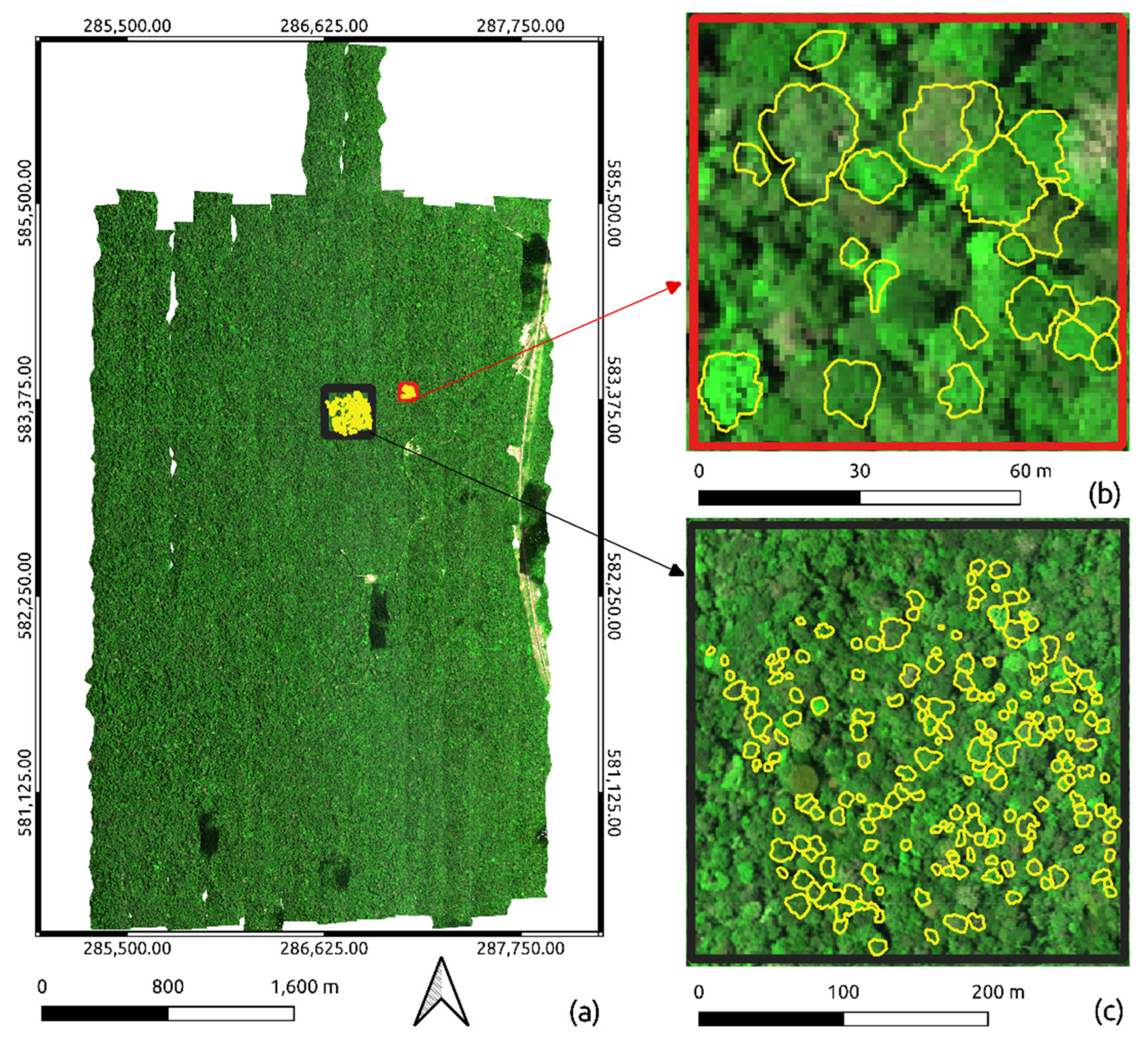
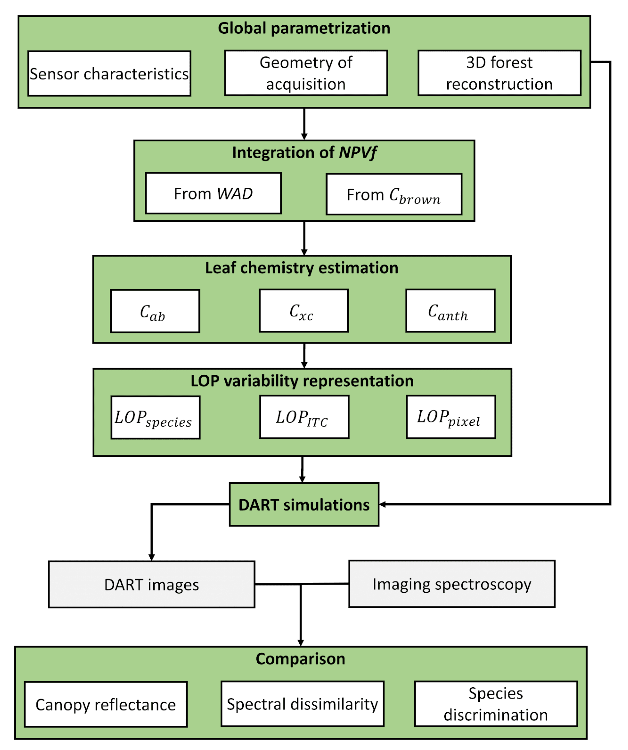
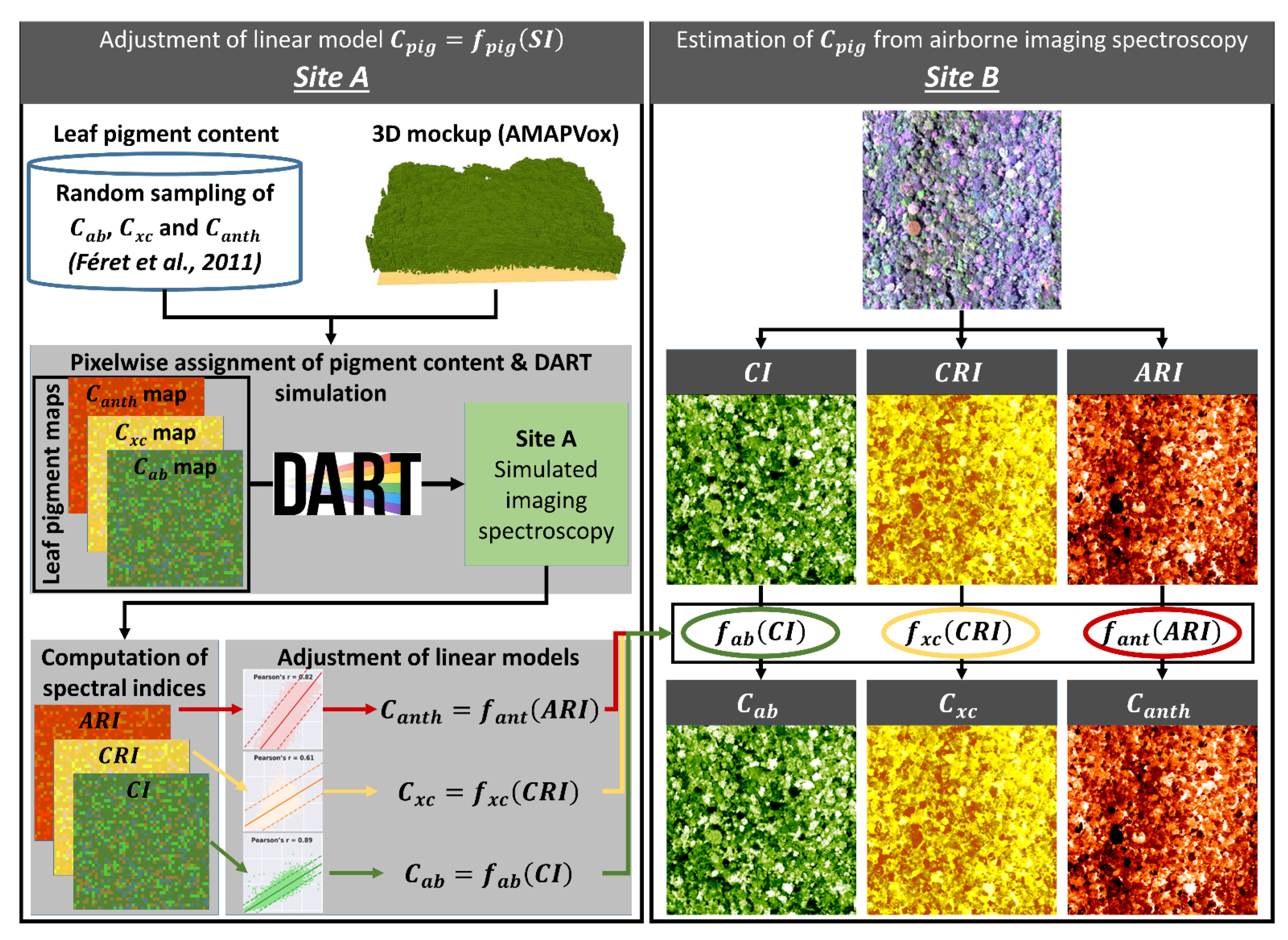
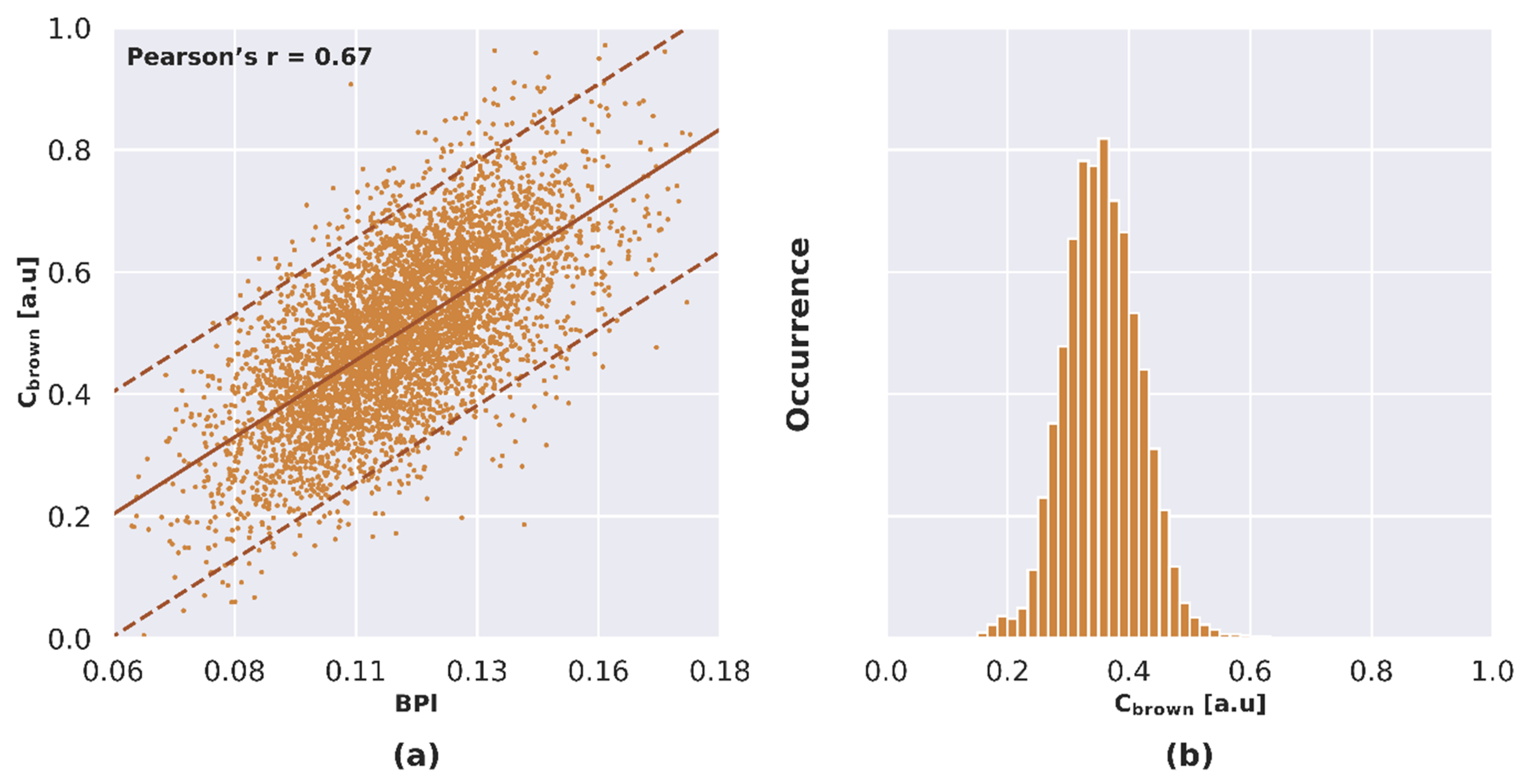
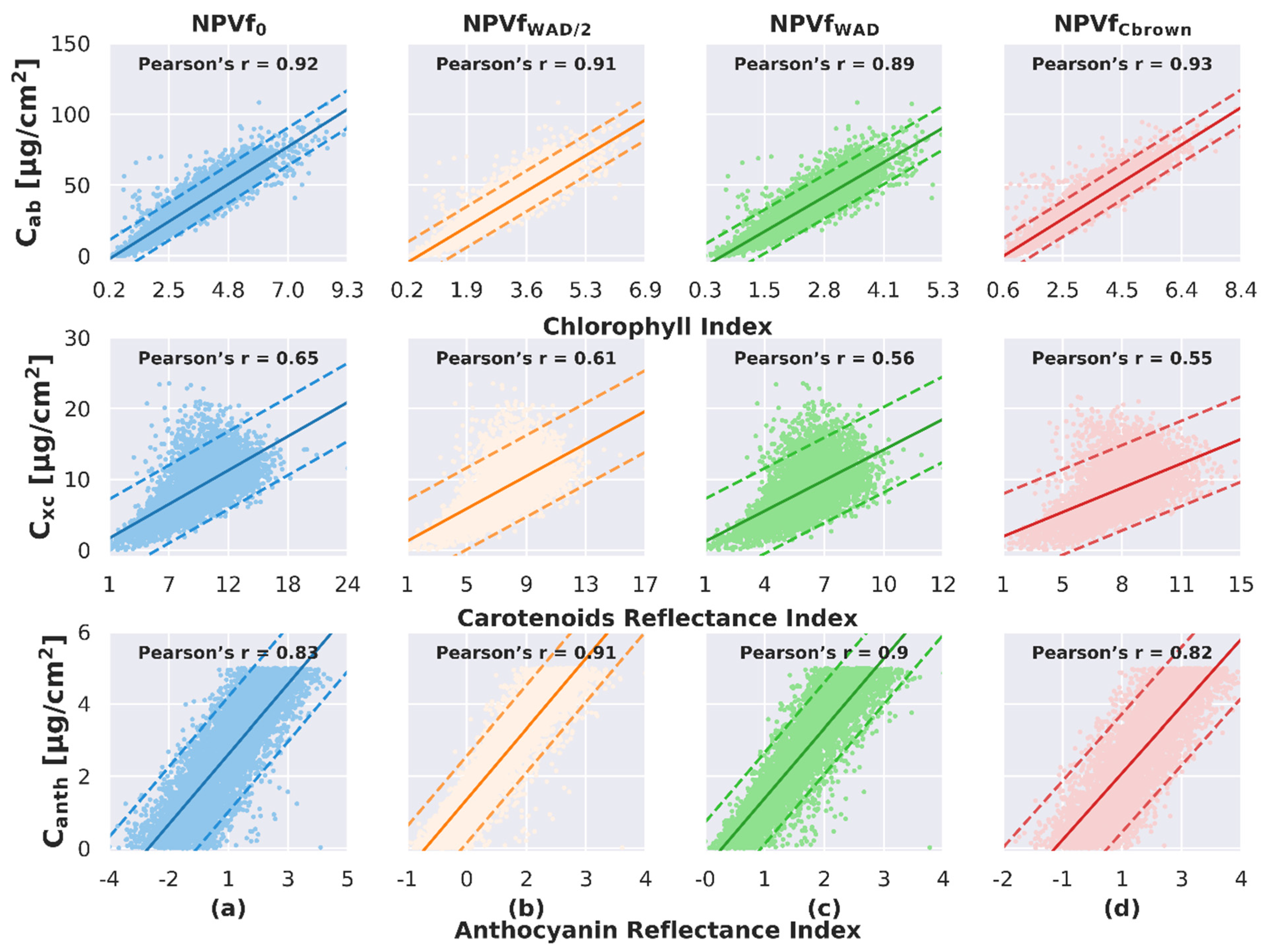
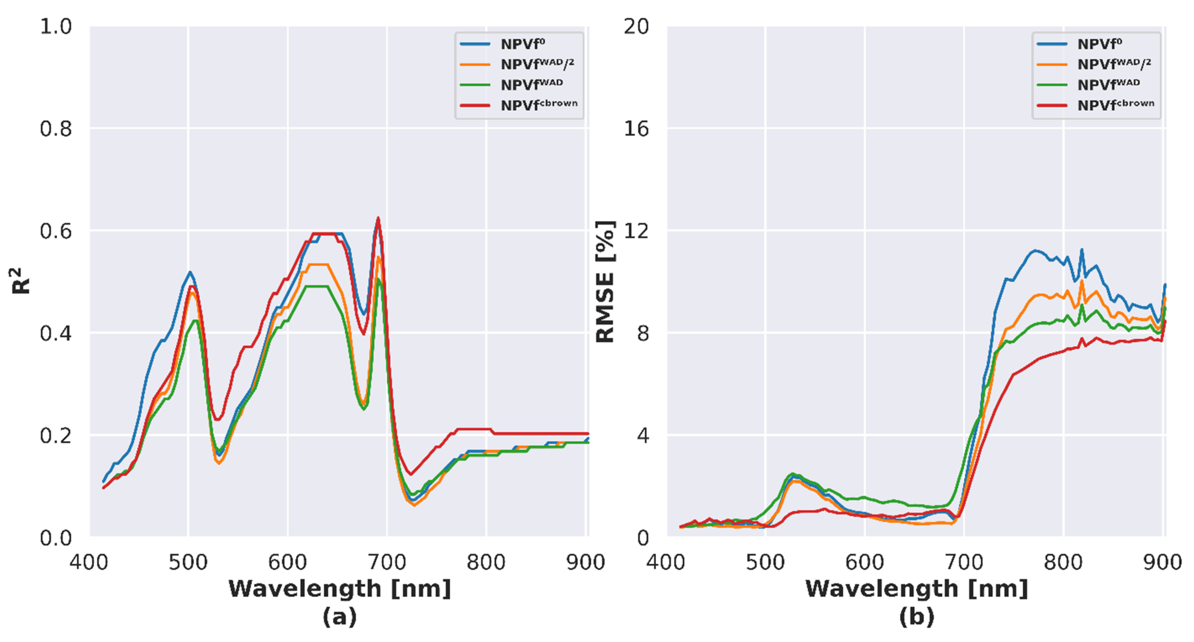
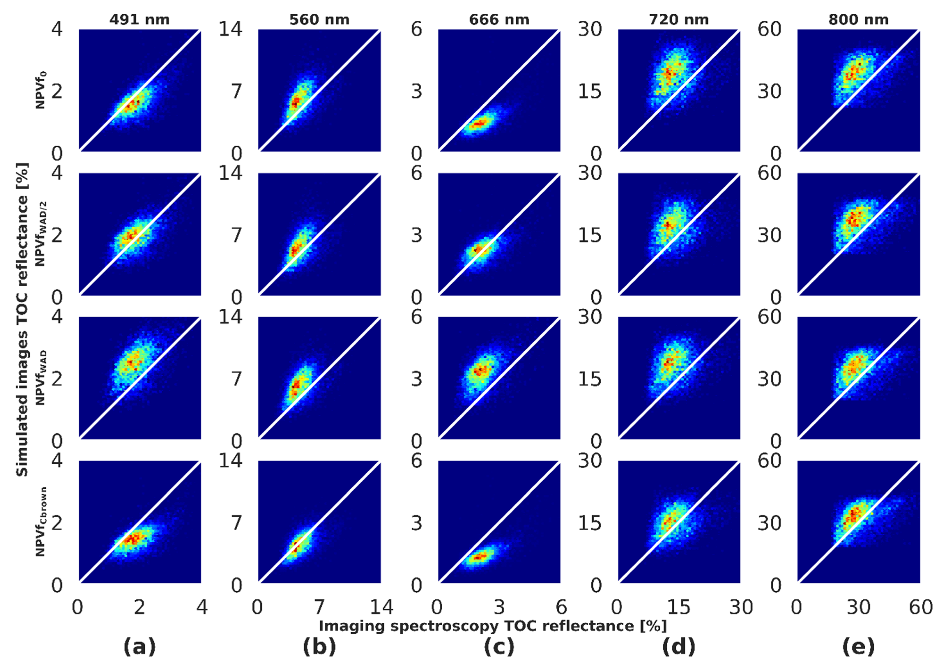
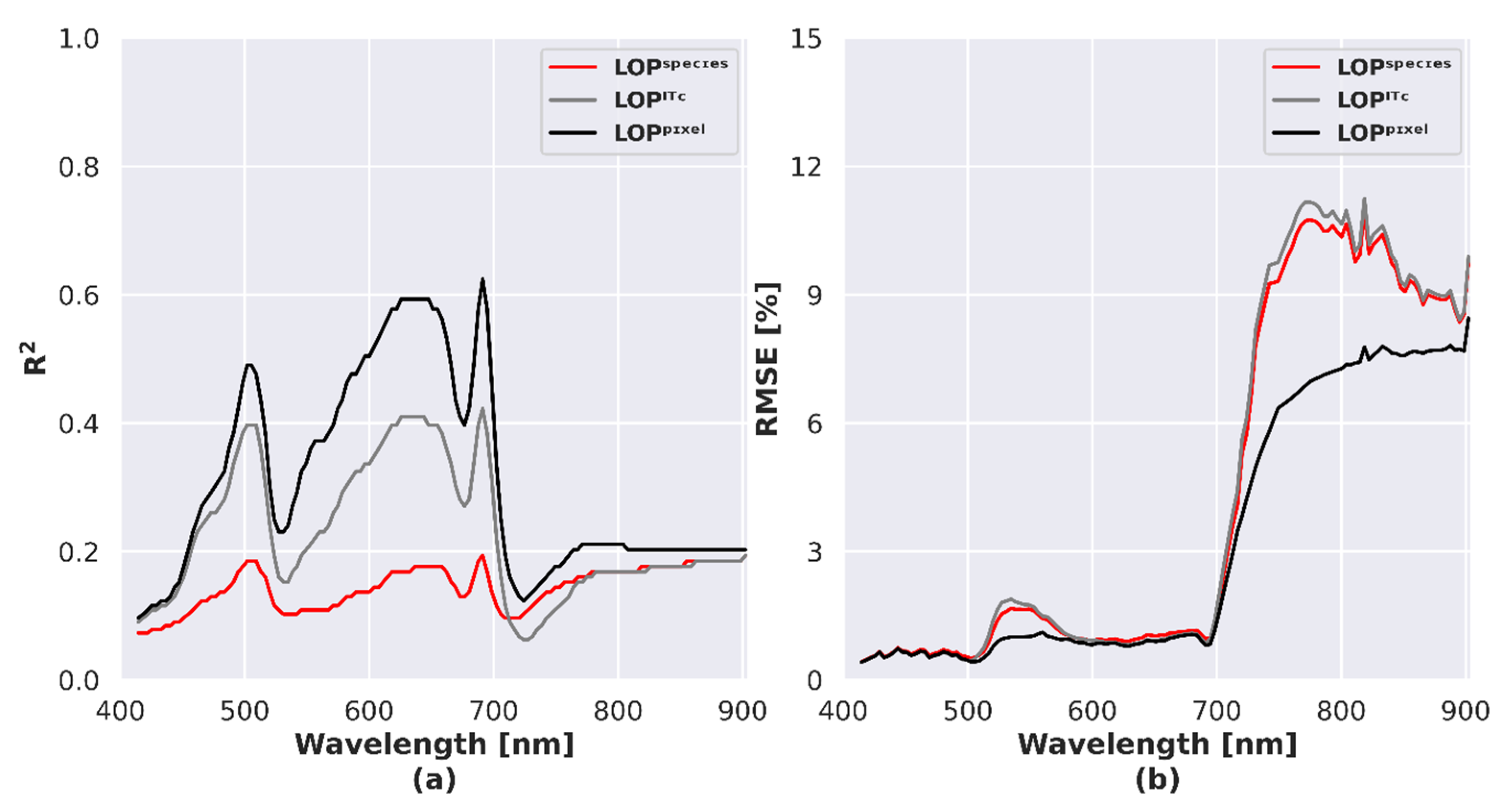
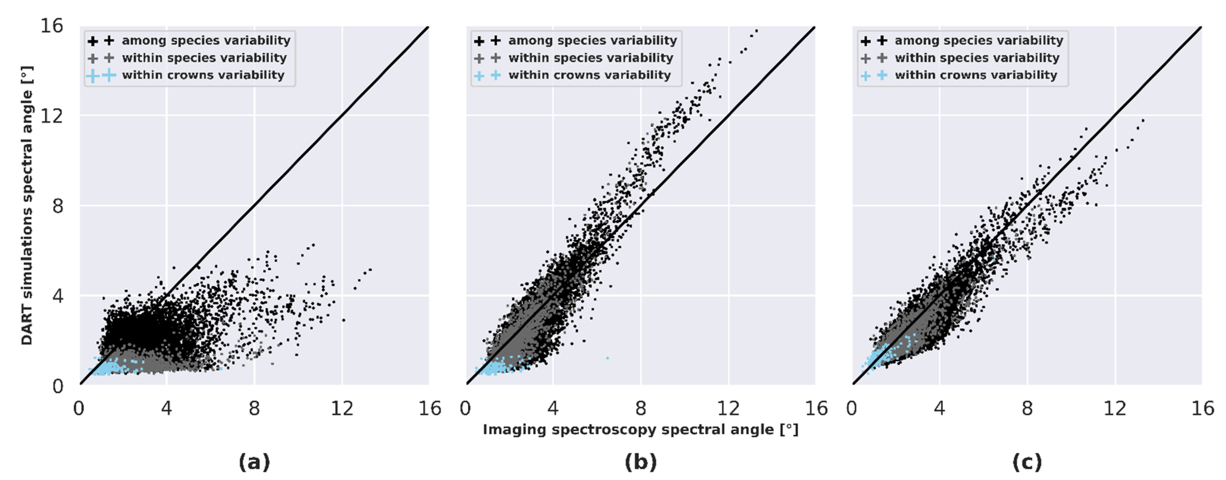
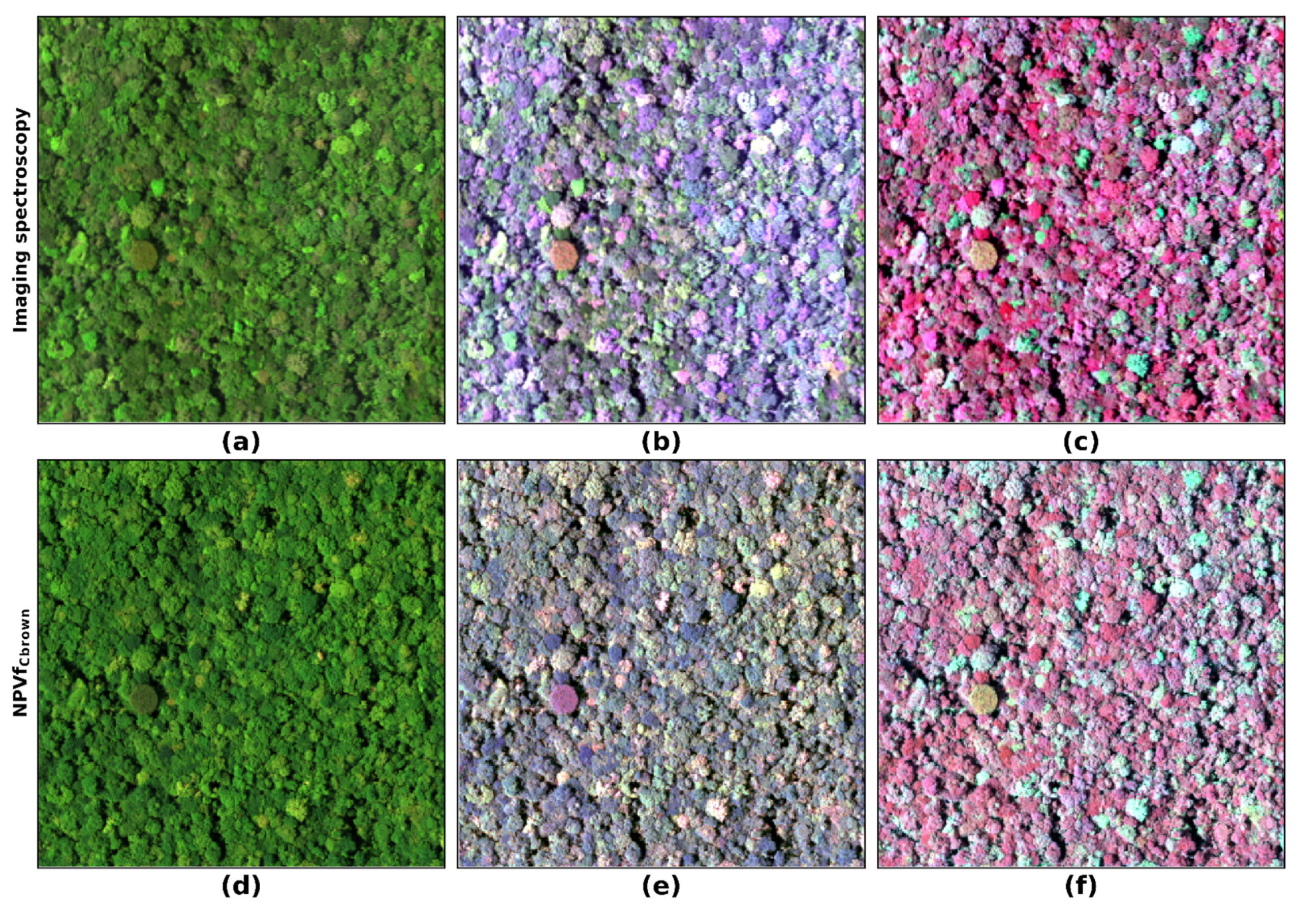
Table 1.
Statistical description of ITCs corresponding to the nine most abundant species delineated in site A and B.
Table 1.
Statistical description of ITCs corresponding to the nine most abundant species delineated in site A and B.
| Species | Number of ITCs | Number of Pixels | Mean Number of Pixels Per ITC |
|---|---|---|---|
| Site A | |||
| Bocoa prouacensis | 1 | 72 | 72 |
| Dicorynia guianensis | 1 | 53 | 53 |
| Eschweilera sagotiana | 5 | 286 | 57 |
| Licania alba | 1 | 83 | 83 |
| Licania heteromorpha | 2 | 44 | 22 |
| Pradosia cochlearia | 2 | 433 | 216 |
| Sextonia rubra | 2 | 223 | 111 |
| Vouacapoua americana | 6 | 387 | 64 |
| Total | 20 | 1581 | 85 |
| Site B | |||
| Dicorynia guianensis (DG) | 11 | 1147 | 104 |
| Eperua falcata (EF) | 45 | 3102 | 68 |
| Eperua grandiflora (EG) | 8 | 694 | 86 |
| Eschweilera sagotiana (ES) | 30 | 1270 | 42 |
| Licania heteromorpha (LH) | 8 | 251 | 31 |
| Moronobea coccinea (MC) | 12 | 609 | 50 |
| Pradosia cochlearia (PC) | 14 | 1538 | 109 |
| Recordoxylon speciosum (RS) | 14 | 944 | 67 |
| Tapura capitulifera (TC) | 20 | 707 | 35 |
| Total | 162 | 10262 | 66 |
Table 2.
Pearson’s correlation coefficient and RMSE computed when comparing spectral dissimilarity from imaging spectroscopy and from DART simulations for the different LOP variability scenarios. Spectral dissimilarity is compared within crowns, within species and among species.
Table 2.
Pearson’s correlation coefficient and RMSE computed when comparing spectral dissimilarity from imaging spectroscopy and from DART simulations for the different LOP variability scenarios. Spectral dissimilarity is compared within crowns, within species and among species.
| Pearson’s r | RMSE [°] | ||||||
|---|---|---|---|---|---|---|---|
| LOP Scenario | LOPspecies | LOPITC | LOPpixel | LOPspecies | LOPITC | LOPpixel | |
| Spectral Dissimilarity | |||||||
| Within Crowns | 0.10 | 0.34 | 0.88 | 0.84 | 0.80 | 0.30 | |
| Within Species | 0.28 | 0.91 | 0.91 | 1.84 | 0.69 | 0.54 | |
| Among Species | 0.48 | 0.93 | 0.92 | 1.75 | 0.81 | 0.67 | |
Table 3.
Pearson’s correlation coefficient comparing LDA classification of DART simulations to imaging spectroscopy for LOP level scenarios. The consistency in correct classification and misclassification is compared between classification results obtained from airborne acquisition and classification results obtained from simulations.
| Confusion Matrix Elements | LOPspecies | LOPITC | LOPpixel |
|---|---|---|---|
| Correct classification | 0.05 | 0.86 | 0.92 |
| Misclassification | −0.04 | 0.71 | 0.79 |
Publisher’s Note: MDPI stays neutral with regard to jurisdictional claims in published maps and institutional affiliations. |
© 2021 by the authors. Licensee MDPI, Basel, Switzerland. This article is an open access article distributed under the terms and conditions of the Creative Commons Attribution (CC BY) license (https://creativecommons.org/licenses/by/4.0/).
Share and Cite
MDPI and ACS Style
Ebengo, D.M.; de Boissieu, F.; Vincent, G.; Weber, C.; Féret, J.-B. Simulating Imaging Spectroscopy in Tropical Forest with 3D Radiative Transfer Modeling. Remote Sens. 2021, 13, 2120. https://doi.org/10.3390/rs13112120
AMA Style
Ebengo DM, de Boissieu F, Vincent G, Weber C, Féret J-B. Simulating Imaging Spectroscopy in Tropical Forest with 3D Radiative Transfer Modeling. Remote Sensing. 2021; 13(11):2120. https://doi.org/10.3390/rs13112120
Chicago/Turabian StyleEbengo, Dav M., Florian de Boissieu, Grégoire Vincent, Christiane Weber, and Jean-Baptiste Féret. 2021. "Simulating Imaging Spectroscopy in Tropical Forest with 3D Radiative Transfer Modeling" Remote Sensing 13, no. 11: 2120. https://doi.org/10.3390/rs13112120
Note that from the first issue of 2016, this journal uses article numbers instead of page numbers. See further details here.