
High-Resolution Rice Mapping Based on SNIC Segmentation and Multi-Source Remote Sensing Images


1
Institute of Applied Remote Sensing and Information Technology, Zhejiang University, Hangzhou 310058, China
2
Institute of Agricultural Resources and Regional Planning, Chinese Academy of Agricultural Sciences, Beijing 100081, China
*
Author to whom correspondence should be addressed.
Remote Sens. 2021, 13(6), 1148; https://doi.org/10.3390/rs13061148
Submission received: 14 December 2020
/
Revised: 4 March 2021
/
Accepted: 16 March 2021
/
Published: 17 March 2021
Abstract
:High-resolution crop mapping is of great significance in agricultural monitoring, precision agriculture, and providing critical information for crop yield or disaster monitoring. Meanwhile, medium resolution time-series optical and synthetic aperture radar (SAR) images can provide useful phenological information. Combining high-resolution satellite data and medium resolution time-series images provides a great opportunity for fine crop mapping. Simple Non-Iterative Clustering (SNIC) is a state-of-the-art image segmentation algorithm that shows the advantages of efficiency and high accuracy. However, the application of SNIC in crop mapping based on the combination of high-resolution and medium-resolution images is unknown. Besides, there is still little research on the influence of the superpixel size (one of the key user-defined parameters of the SNIC method) on classification accuracy. In this study, we employed a 2 m high-resolution GF-1 pan-sharpened image and 10 m medium resolution time-series Sentinel-1 C-band Synthetic Aperture Radar Instrument (C-SAR) and Sentinel-2 Multispectral Instrument (MSI) images to carry out rice mapping based on the SNIC method. The results show that with the increase of the superpixel size, the classification accuracy increased at first and then decreased rapidly after reaching the summit when the superpixel size is 27. The classification accuracy of the combined use of optical and SAR data is higher than that using only Sentinel-2 MSI or Sentinel-1 C-SAR vertical transmitted and vertical received (VV) or vertical transmitted and horizontal received (VH) data, with overall accuracies of 0.8335, 0.8282, 0.7862, and 0.7886, respectively. Meanwhile, the results also indicate that classification based on superpixels obtained by SNIC significantly outperforms classification based on original pixels. The overall accuracy, producer accuracy, and user accuracy of SNIC superpixel-based classification increased by 9.14%, 17.16%, 27.35% and 1.36%, respectively, when compared with the pixel-based classification, based on the combination of optical and SAR data (using the random forest as the classifier). The results show that SNIC superpixel segmentation is a feasible method for high-resolution crop mapping based on multi-source remote sensing data. The automatic selection of the optimal superpixel size of SNIC will be focused on in future research.
1. Introduction
High-resolution satellite images can provide a more precise and accurate spatial distribution of crop planting plots, thus providing important reference information for the implementation of precision agriculture and the formulation of agricultural policies [1,2]. However, crop mapping based on high-resolution satellite images is restricted by the difficulties in obtaining time-series high-resolution satellite data and appropriate classification methods [3].
High-resolution satellite imagery can provide clearer and richer ground details, thus providing advantages for crop mapping. However, it generally has a narrower width and a long revisit period, making it difficult to obtain high-resolution images with long time series, especially in cloud-prone environments [4,5]. On the contrary, a medium resolution satellite generally has a short revisit period, which can be used to acquire multi-temporal remote sensing images that will provide phenological information for crop mapping, especially synthetic aperture radar (SAR) data has the ability to obtain images under all-weather conditions [6,7]. The combination of high-resolution imagery and medium resolution multi-temporal remote sensing imagery can provide a reliable satellite data source for fine crop mapping [8].
In addition, the traditional pixel-based classification method used for high-resolution satellite image classification suffers from the salt and pepper phenomenon of the classification results, which reduces the integrity of the crop field [9,10]. Image segmentation is a kind of technology that partitions an image into multiple segments. Many studies have shown that image segmentation technologies such as Multi-Resolution Segmentation (MRS), Simple Linear Iterative Clustering (SLIC), and Simple Non-Iterative Clustering (SNIC) provide a new and evolving paradigm specifically for high-resolution remote sensing images compared to the pixel-based classification [9,11,12,13,14]. According to the segmentation results, image segmentation can be classified into two types: one is to extract field boundaries, which provide basic data for parcel-level crop monitoring [15,16]; the other is to simply an image into small clusters of connected pixels that shared common characteristics, namely those of objects or superpixels [11,17,18]. It avoids the struggle with semantics as it does not need to consider the meaning of the object or superpixel. Taking advantage of its simplicity and efficiency, more attention has been paid to superpixel segmentation lately [12,19]. Simple Non-Iterative Clustering (SNIC) is the state-of-the-art superpixel segmentation algorithm developed from Simple Linear Iterative Clustering (SLIC). It has the advantages of less memory consumption and faster speed. It shows great potential in crop mapping [20,21], land use–land cover classification [22,23], hyperspectral data classification [24] and wetland inventory [25]. Zhang et al. [26] mapped up-to-date paddy rice extent at 10 m resolution through the integration of optical and SAR images and the SLIC method was used to improve the pixel-based classification. Csillik [11] found that SLIC superpixel-based classification had similar or better performance when compared to multi-resolution segmentation (MRS) based classification. However, the research on high-resolution satellite image segmentation using the SNIC method is still insufficient. Especially, the research of superpixel-based crop mapping based on combining high-resolution satellite images and multi-source medium resolution imagery is still lacking. In addition, the influence of the superpixel size, which is the key parameter of the SNIC method, on the classification accuracy, is still unknown. Previous studies mainly focused on obtaining the optimal value from several alternative values [22,23], and to the best of our knowledge, there are still no detailed studies on the change of classification accuracy with the change of superpixel size.
In this study, a high-resolution GF-1 pan-sharpened image was partitioned into multiple superpixels based on the SNIC method and then the features of each superpixel were calculated by averaging the values of all pixels of multi-source time-series medium resolution images contained in the superpixel, to carry out rice mapping in the study area based on a random forest (RF) classifier. The objectives of this study are as follows: (1) Studying the variation of classification accuracy with the increase of the superpixel size parameter of the SNIC method. (2) Exploring the influence of different combinations of remote sensing data on the classification accuracy based on the SNIC method. (3) Comparing the performance of superpixel-based classification and pixel-based classification to study the necessity of superpixel-based crop mapping based on multi-source satellite images.
2. Materials
2.1. Study Area
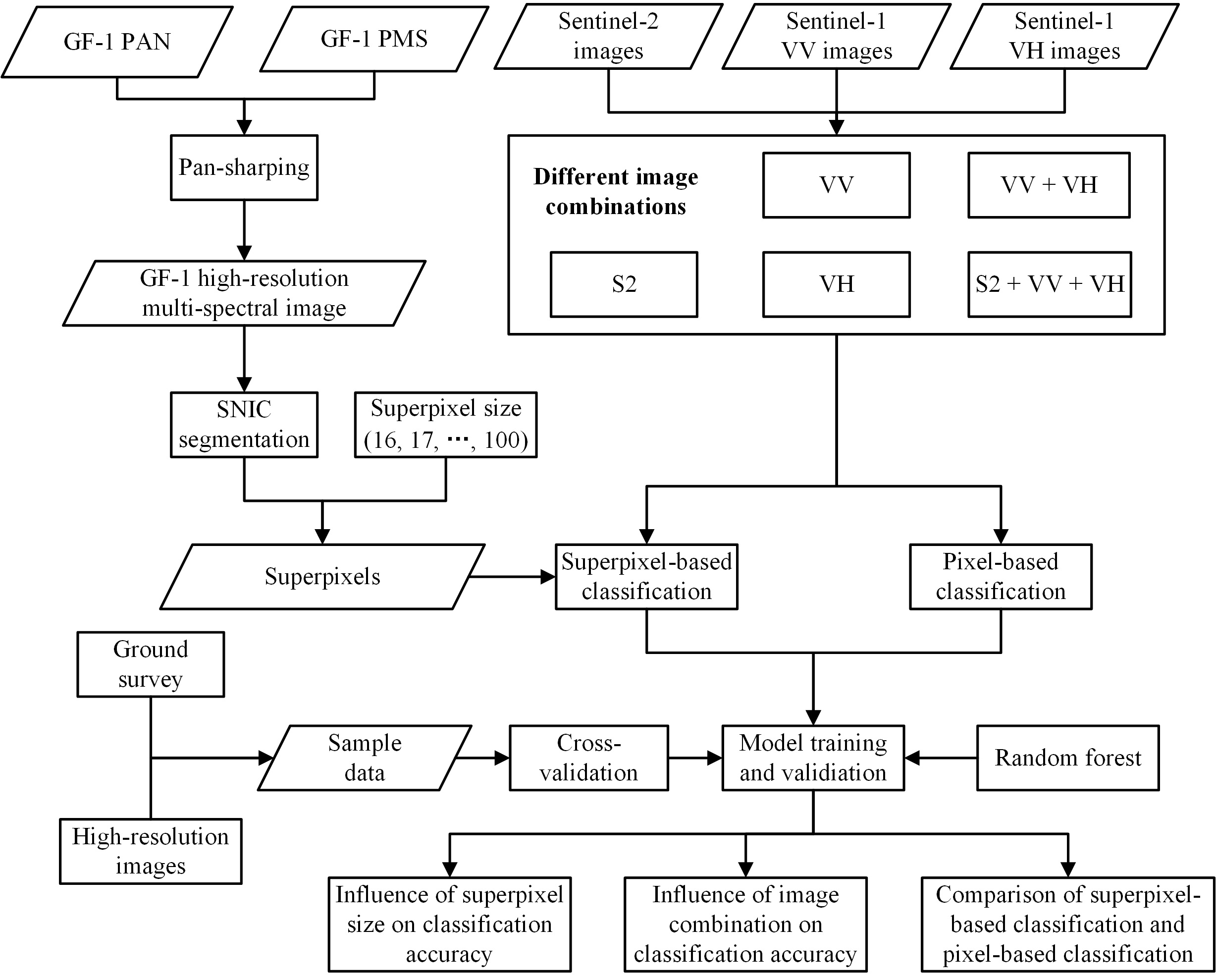
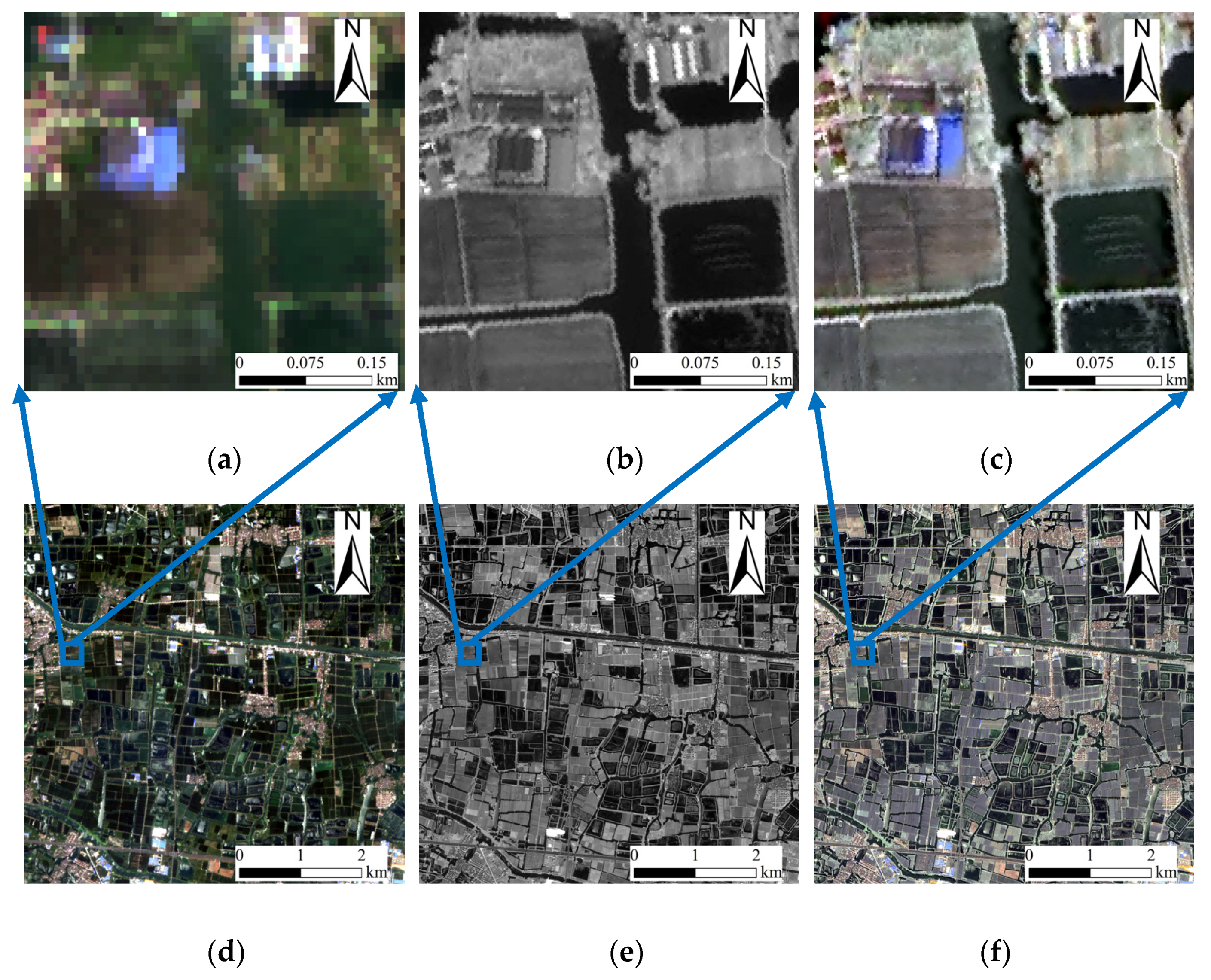
The study area is located in Xinghua City, Jiangsu Province, East China (Figure 1). The total area is about 33 km². The cropping system in the study area is mainly characterized by two crops a year and paddy rice is the main summer crop whose growing season starts from May to November. The average sowing date of paddy rice in the study area is May 26, the average elongation date is August 6, the average heading date is September 1, and the average maturity date is October 16.
2.2. Remote Sensing Data and Pre-Processing
Three kinds of remote sensing images were selected and pre-processed in order to carry out rice mapping. These include high-resolution GF-1 panchromatic/multi-spectral (PMS) images, Sentinel-2 Multispectral Instrument (MSI) images, and Sentinel-1 C-band synthetic aperture radar (SAR) instrument (C-SAR) images.
2.2.1. Remote Sensing Data
GF-1 PMS data were acquired from the China Center for Resources Satellite Data and Application (CRESDA). In this study, the image acquired on 24 July 2020, was used. The characteristics of the GF-1 PMS data are shown in Table 1.
Sentinel-2 is one of the Earth Observation (EO) missions launched by the European Space Agency (ESA). The mission comprises the twin’s satellite (Sentinel-2A and 2B) with a temporal resolution of five days. All the Sentinel-2 MSI data employed over the study area were provided by ESA. These data are freely available at (https://scihub.copernicus.eu, accessed on 10 December 2020). The images used were from 1 May 2017 to 10 December 2017. As the coastal aerosol (B1), water vapor (B9), and cirrus bands (B10) have a coarse resolution, they were abandoned in this study (Table 2). Finally, a total of 43 Sentinel-2 MSI images were collected and used in the study.
Sentinel-1 is a two-satellite constellation (Sentinel-1A and Sentinel-1B) performing C-band SAR imaging of the Earth regardless of the weather condition. It operates in Interferometric Wide (IW) swath mode in the study area that allowing combining a large swath width (250 km) with a moderate geometric resolution (5 m by 20 m). The vertical transmitting and vertical receiving (VV) and vertical transmitting and horizontal receiving (VH) polarisation data from the IW swath mode were used over the study area. A total of 44 Sentinel-1 C-SAR images over the study area from April 2017 to December 2017 were provided by ESA.
2.2.2. Pre-Processing of Remote Sensing Data
The pre-processing steps of GF-1 PMS images include geometric and atmospheric corrections, and pan-sharpening of multi-spectral and PAN images. The Rational Polynomial Coefficients (RPC) model was used for geometric correction of GF-1 images, and the parameters of the RPC model was downloaded together with the GF-1 images [27]. Shuttle Radar Topography Mission (SRTM) data were employed as the source of Digital Elevation Model (DEM) for geometric correction based on the RPC model. As the study area is located in a plain area with an attitude between 1 and 2 m, the 30-m resolution SRTM DEM is accurate enough for the RPC orthorectification of GF-1 PMS data. The Fast Line-of-sight Atmospheric Analysis of Spectral Hypercubes (FLAASH) was applied to GF-1 images for atmospheric correction. CRESDA provides the parameters used for FLAASH (flight time, scene center location et al.) and sensors’ spectral response functions.
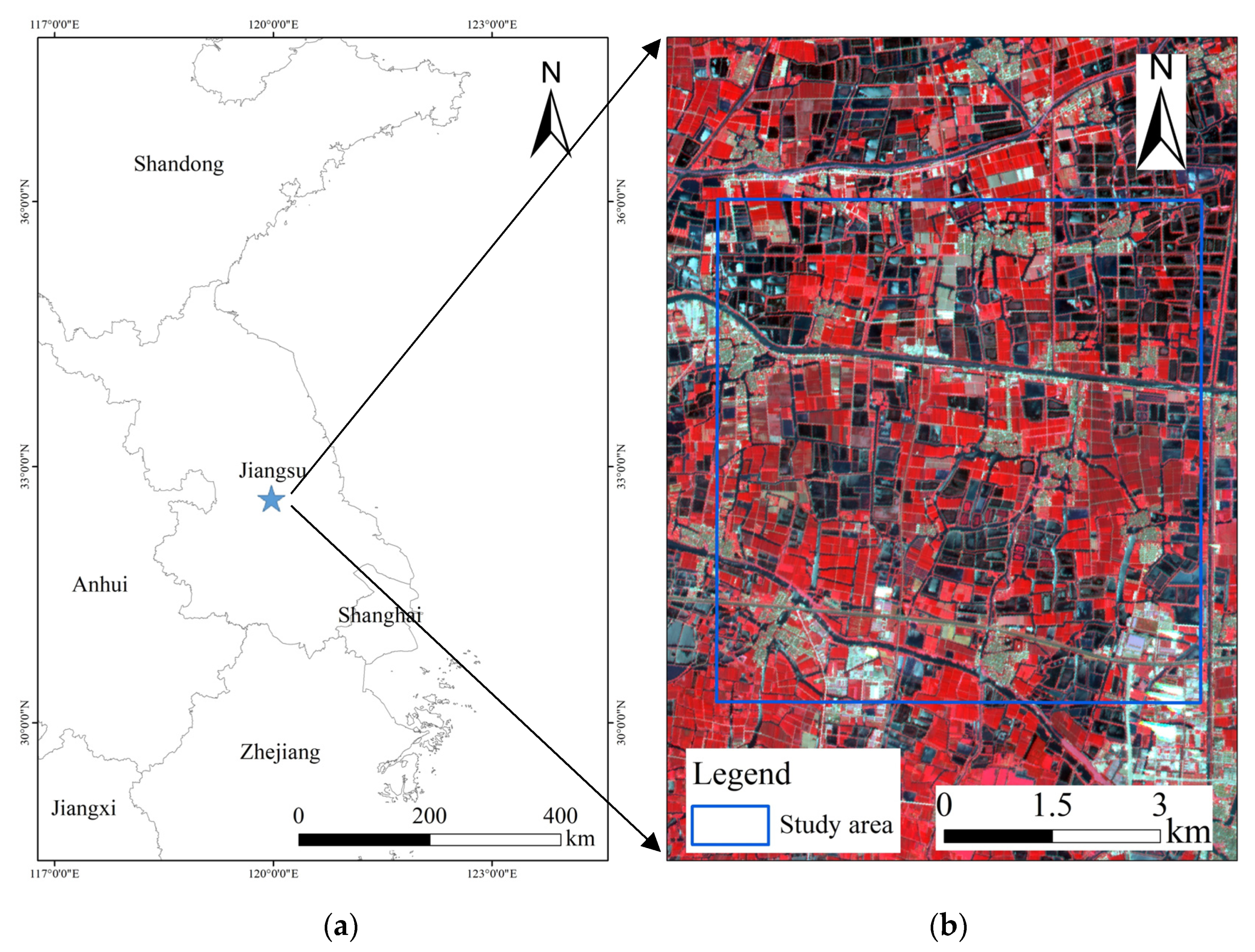
Pan-sharpening is a widely used image fusion method. It projects the original multi-spectral image into a new space and replaces the component that represents the spatial information with the high-resolution panchromatic image. It performs back projection to obtain a pan-sharpened high-resolution multi-spectral image [28]. The Gram–Schmidt method was selected to perform pan-sharpening in this study. The method uses the spectral response functions of a given sensor to create an accurate pan-sharpened image [29]. The final pan-sharpened 2 m resolution multi-spectral GF-1 image is provided in Figure 2. It clearly illustrates that the pan-sharpened image has more accurate boundary information about the croplands, buildings, water bodies and other objects, which significantly improves the ability to distinguish ground objects compared with the raw GF-1 multi-spectral image. All the pre-processing steps of GF-1 PMS images were carried out in ENVI software (Exelis Visual Information Solutions., Broomfield, CO, USA) 5.3.1.
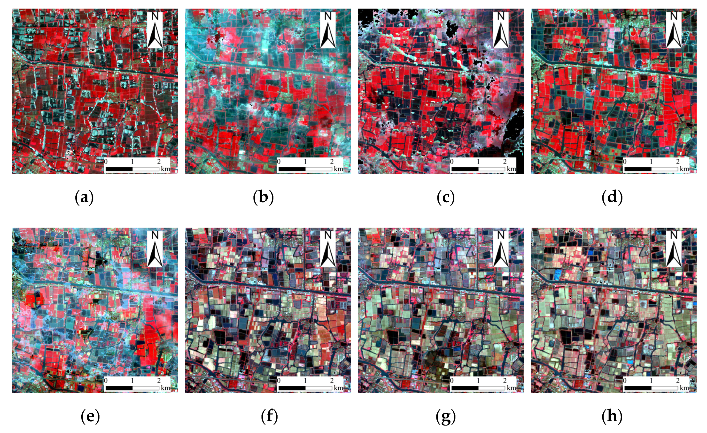
The original data of Sentinel-2 MSI are level-1C top of atmosphere reflectance data, which were then converted into surface reflectance data using the sen2cor (v2.4.0) tool provided by ESA [9]. Then, based on the quality assessment (QA) bands, we carried out a cloud mask of the Sentinel-2 MSI surface reflectance data. Then, a full coverage of clear-sky image was produced using the mean value of all the masked images in a certain period. Based on clear-sky from April to December, we obtained the clear-sky composite images of the following months (July, August, and September). The first half of October, the second half of October, the first mid-November, the second half of November, and finally, the first ten days of December were also acquired (Figure 3).
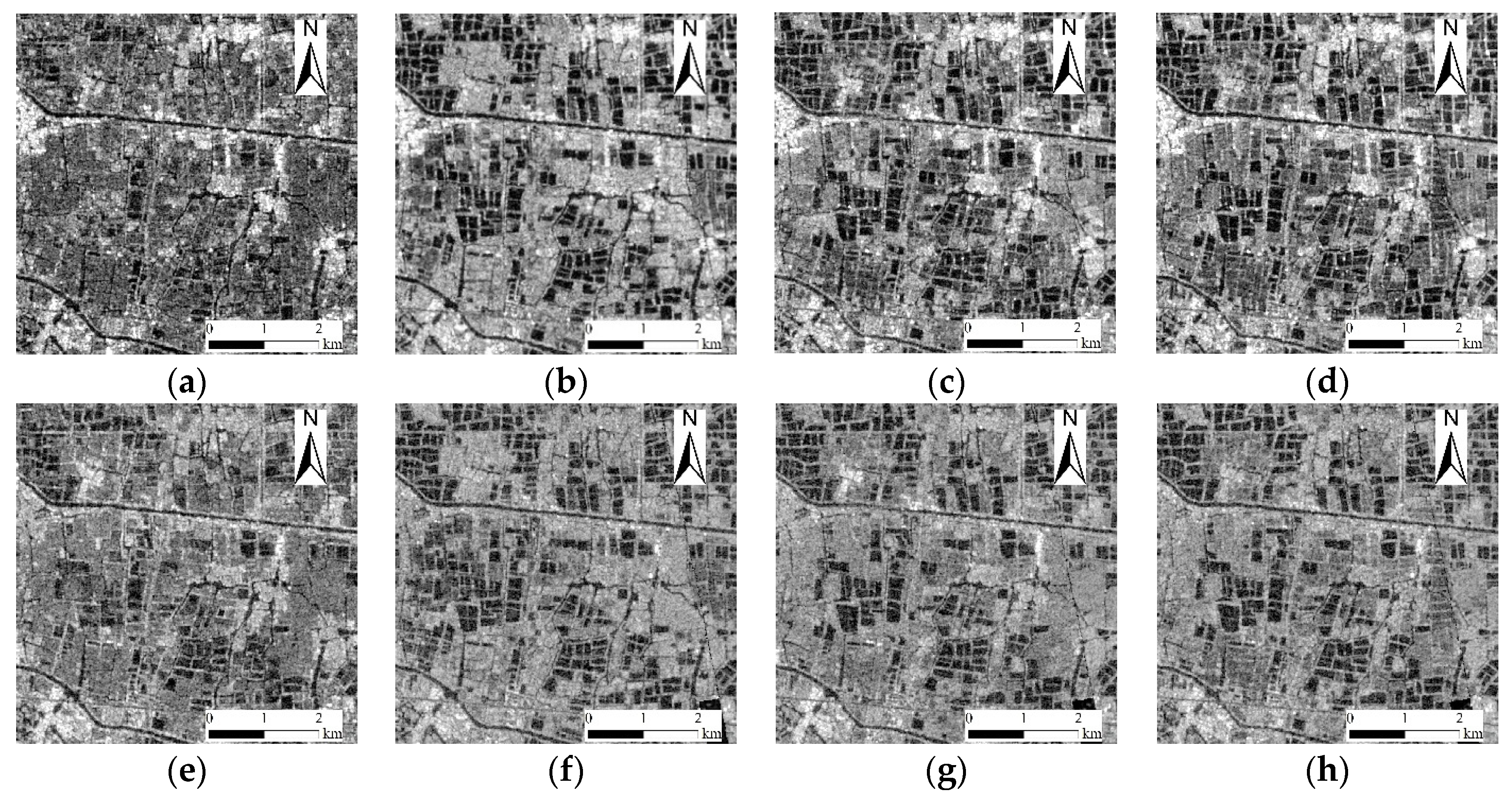
All the Sentinel-1 C-SAR data were pre-processed using Sentinel Application Platform (SNAP) software provided by ESA [6]. Firstly, we applied precise orbit files gotten from the metadata to all images. Then, thermal noise removal and a Refined Lee speckle filtering was used to reduce the speckle noise. Then, we calibrated the images to obtain sigma naught (σ0) backscatter coefficients (dB). Finally, we performed a Range Doppler terrain correction based on SRTM DEM data and the resolution of the images was converted to 10 m. In this study, we divided each month from April to December into three periods: the first ten days, the second ten days, and the rest of the month. Based on the mean value composite technology, the mean VV and VH image for each period was produced to reduce the speckle noise of the raw images and the number of input images. Finally, 27 Sentinel-1 VV and VH images were produced and used in this study (Figure 4).
2.3. Ground Survey and Sampling
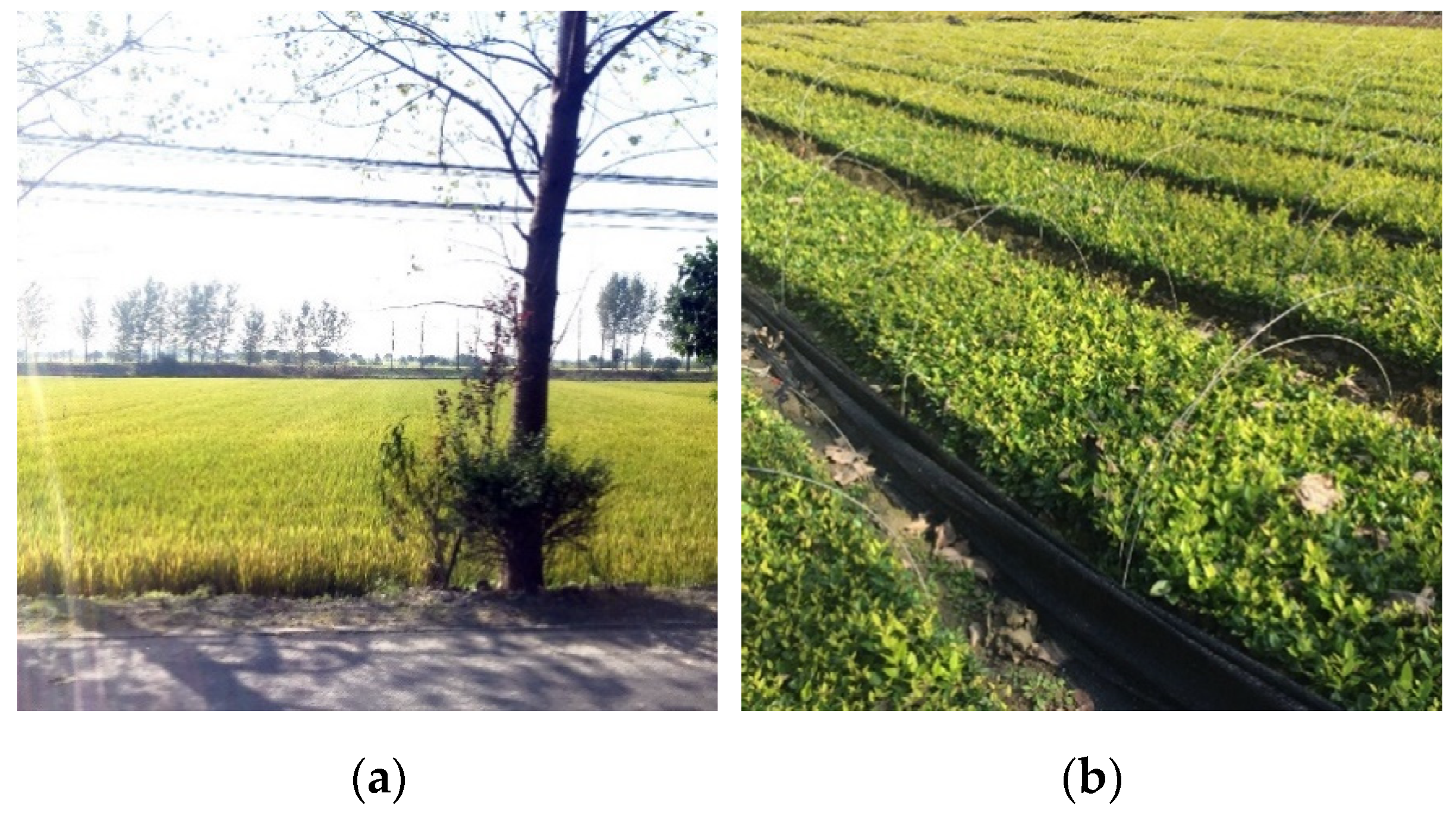
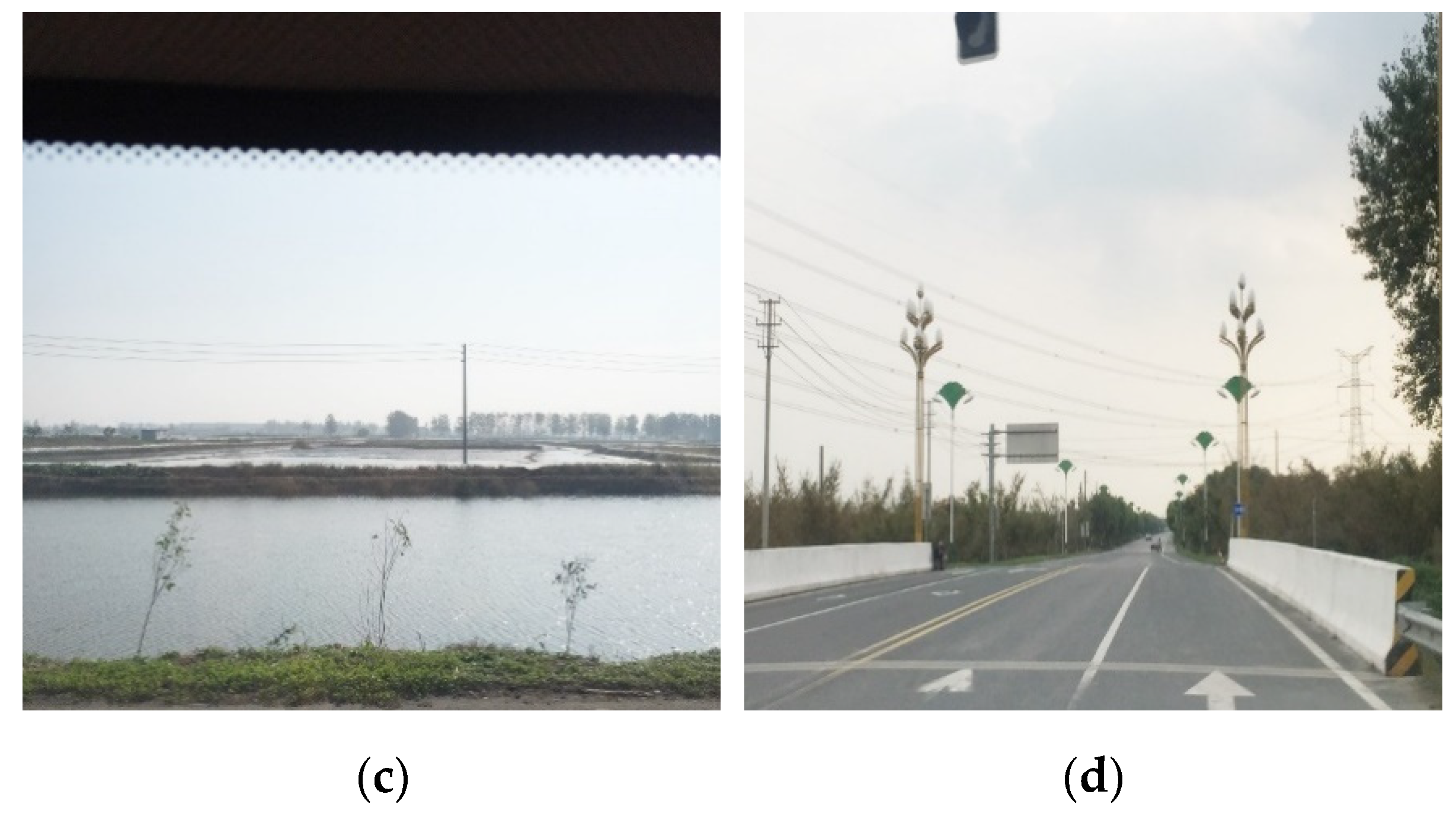
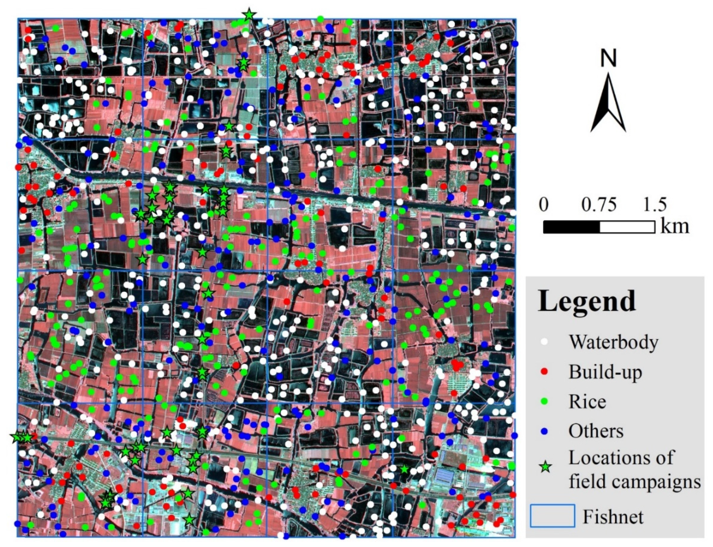
Field campaigns were carried out in October 2017 and a series of ground survey data were collected which includes accurate GPS locations, crop types, and photos (Figure 5). Based on the knowledge obtained from the field survey, as well as the use of high-resolution GF-1 pan-sharpened image and Google Earth data, we selected a large number of sample points in the study area (Figure 6). A fishnet covering the whole study area was created to assist in generating random sample points. The fishnet consists of 16 rectangles of the same size. In total, 63 random points were generated randomly inside each rectangle. Thus, a total of 1008 sample points were generated. These sample points were classified based on broad land-cover classes such as waterbody, built-up area, paddy rice, and others. The numbers of sample points for each class are 431, 121, 213, and 243, respectively.
3. Methodology
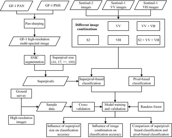
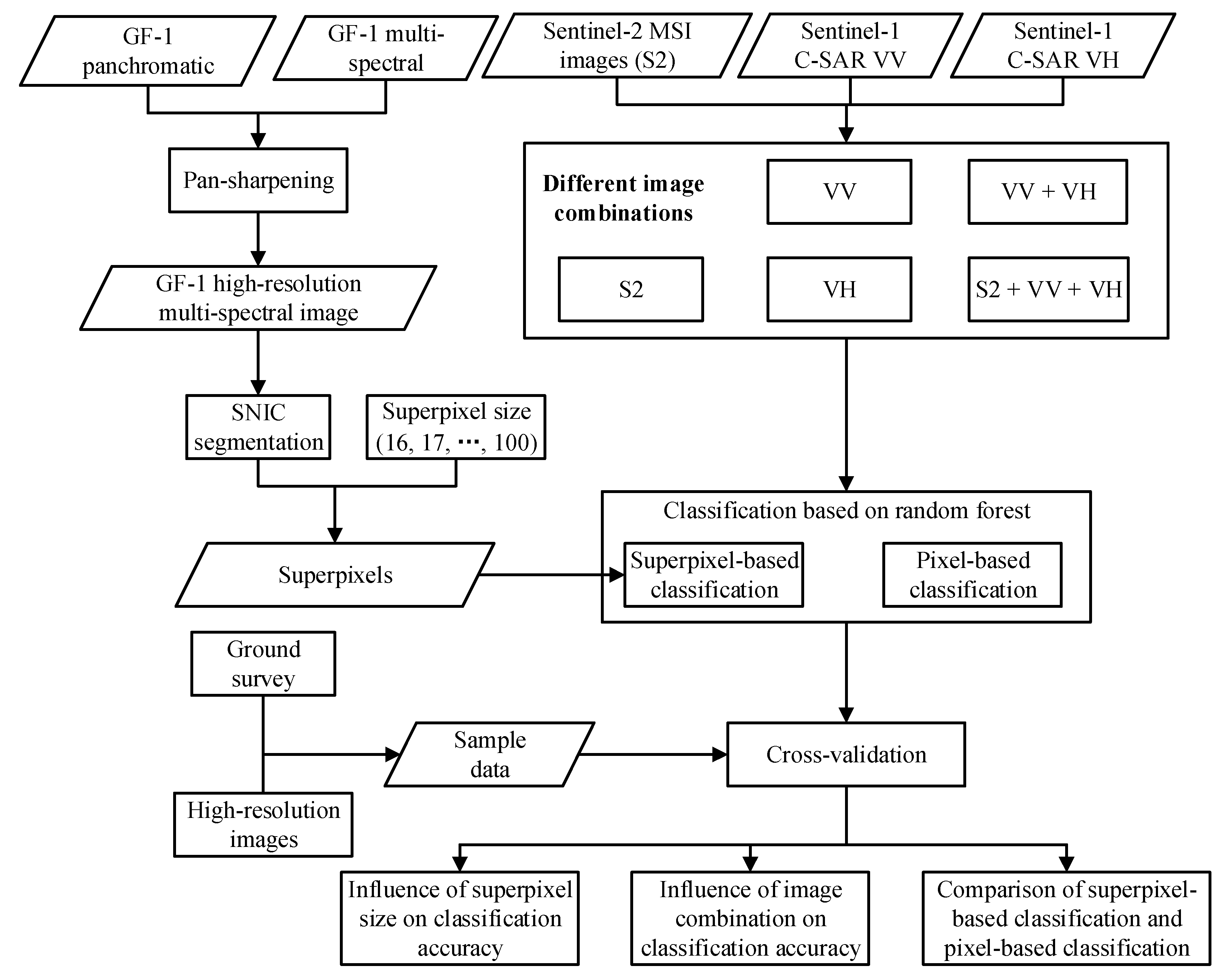
Five image classification schemes (Table 3) were designed to learn the influence of image combinations on classification accuracy based on SNIC (Figure 7). GF-1 pan-sharpened image was used for SNIC segmentation and segmented into a series of superpixels based on different superpixel sizes from 16 to 100 with an interval of 1. The features of each superpixel were obtained from images of each image combination. The value of each feature of each superpixel was calculated by averaging the values of all the pixels contained in the superpixel. Random forest was used as the classifier. The accuracies of each image combination and each superpixel size were calculated by sample data. Thus, the optimal image combination and superpixel size for rice mapping could be obtained.
Besides, in order to compare the performance of the SNIC superpixel-based classification with the pixel-based classification, we also carried out pixel-based classification based on these five image combinations and applied a random forest classifier. We evaluated their accuracies to explore the impact of SNIC on remote sensing image classification.
Several accuracy metrics were selected to evaluate the accuracies of classification results, including overall accuracy (OA), user accuracy (UA), and producer accuracy (PA) [30]. Four-fold cross-validation was used as the evaluation method, namely that of randomly partitioning the original sample dataset into 4 equally sized sub-datasets [31]. Then, one sub-dataset was retained as the test dataset, and the remaining three sub-datasets were used as training data. This process is repeated four times, with each of the four sub-datasets used exactly once as the validation dataset. A final accuracy was calculated by averaging all four results.
3.1. Superpixel Segmentation Based on Simple Non-Iterative Clustering (SNIC)
SNIC is the state-of-the-art superpixel segmentation algorithm based on SLIC [32]. It has the advantages of non-iterative, requiring lesser memory, and faster and enforcing connectivity from the start. It owes its success as a preprocessing algorithm to its simplicity, its computational efficiency, and its ability to generate superpixels that satisfy the requirements of good boundary adherence and limited adjacency [17].
SNIC uses a regular grid to generate K initial centroids in the image plane, and then K corresponding elements are created [24]. Each element in the SNIC includes spatial position, CIELAB color, superpixel label and the distance of the superpixel centroid to the candidate pixel. The K elements are then pushed into a priority queue Q. While Q is not empty, it always pops out the element whose distance is the smallest. For each connected neighbor pixel of the popped element, a new element is created if the pixel has not been labeled yet and assigning to it the distance from the connected centroid and the label of the connected centroid. Then, it is pushed into the queue. Each new element pushed into the queue is used to perform an online update of the corresponding centroid value. When all the pixels of the image have been labeled and Q has been emptied, the SNIC algorithm then terminates [17].
The number of the initial centroids K is the main user user-defined parameter of SNIC. It determines the size s of a superpixel, which could be calculated as follows:
where N is the number of pixels in the image.
3.2. Classification Based on Random Forest
Random forest (RF) is a classification and regression model; it consists of a large number of individual uncorrelated decision trees [33]. The final result is an average of all individual tree outputs. It applies the bagging technique in both samples and features. It repeatedly selects a random subset with the replacement of the training set and trains a decision tree based on the randomly selected samples and a random subset of the features. The remaining samples could be used to calculate the accuracy of the decision tree. The importance of each individual tree could be assessed by the Gini index. Random forest is a robust and easy to use machine learning algorithm which has been proved accurate and has the ability to overcome overfitting [34].
4. Results
4.1. Rice Mapping Based on SNIC and Multi-Source Remote Sensing Images
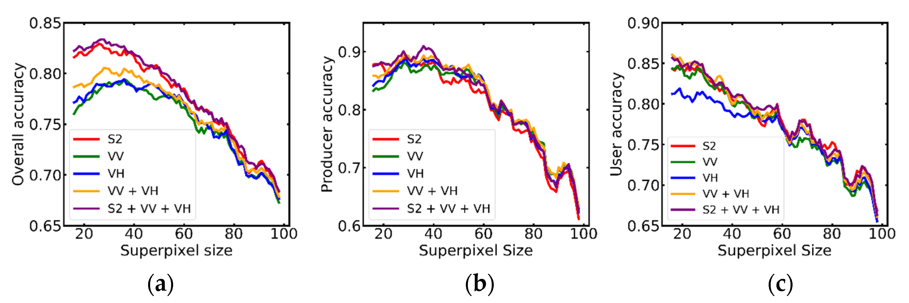
The classification accuracies of all the five image combinations increase at first, then reach a peak when the size of the superpixel is around 30, and then progressively decrease (Figure 8). A smaller SNIC superpixel size caused an over-segmentation phenomenon; that is, one object which is composed of a collection of pixels with similar attributes is segmented into several different superpixels. In addition, a smaller superpixel makes it hard to integrate the information from coarse resolution optical images and SAR images, thus reducing the classification accuracy. On the other hand, a larger superpixel size caused an under-segmentation phenomenon, that is, the objects with different attributes are wrongly segmented into the same superpixel, which will cause serious misclassification.
Figure 8 also indicates that the SNIC superpixel-based classification based on the combination of optical and SAR images achieves the highest classification accuracy. It reaches its highest accuracy when the superpixel size is 27. Its overall accuracy, producer accuracy, and user accuracy reach 0.8335, 0.8478, 0.8930, respectively. The performance of S2 + VV + VH is better than that of S2 optical images alone. This is mainly because June and July were the key periods of rice transplanting in this area, as well as the critical phenological period of rice mapping. However, due to cloud obstruction, there are no clear-sky optical images in this period. This gives the SAR data an advantage over optical to obtain images under all weather conditions. The combination of optical and SAR images can improve the classification accuracy in the cloud-prone area.
4.2. Comparison of SNIC Superpixel-Based Classification and Pixel-Based Classification
Based on the optimal superpixel size achieved above (27), SNIC superpixel-based classification in the study area was carried out based on the five image combinations. Meanwhile, the pixel-based classification was performed using the same datasets. Cross-validation was used to assess the accuracy of the classification.
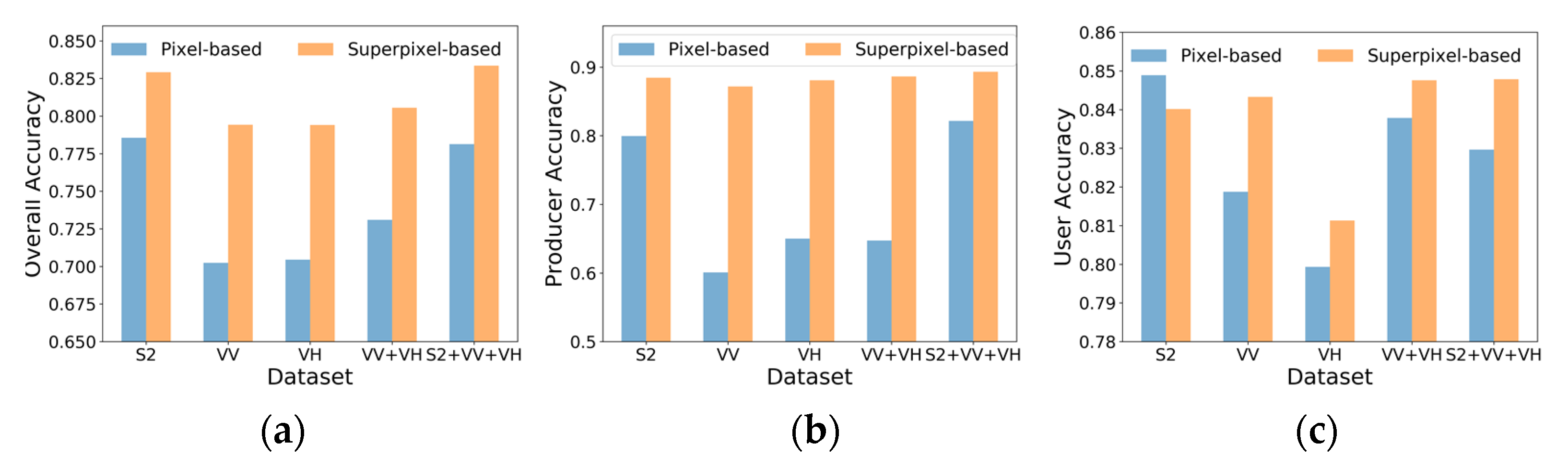
Figure 9 shows that the SNIC superpixel-based classification is significantly outperformed the pixel-based classification for all five datasets. The OA, PA and UA increased by 9.14%, 27.35% and 1.36% on average, respectively. Especially for the rice mapping based on SAR data, the OA, PA and UA of the superpixel-based classification method are improved by 11.20%, 39.14% and 1.89% on average, respectively. This is due to the pixel-based classification method is significantly affected by the speckle noise of the SAR images (Figure 4). Meanwhile, the superpixel uses the average value of all pixels inside the superpixel, thus reducing the negative impact of speckle noise and improving the accuracy.
5. Discussion
Superpixel size has a great impact on the classification accuracy of crop mapping based on SNIC and should be chosen carefully. If the superpixel size is too large, a superpixel may contain more than one class, which will reduce the classification accuracy (Figure 8). When the superpixel size is too small, the efficiency of superpixel segmentation will be reduced, and a too-small superpixel generated from a high-resolution satellite image may only contain a few or even only one pixel of medium resolution satellite images.
Figure 8 implies that the classification of S2 optical satellite images is more robust than that of SAR images. The overall accuracy of S2 is significantly higher than that of VV, VH or VV + VH. This is essential because the optical images contain more spectral information than SAR images which can effectively improve ground object recognition. Moreover, speckle noise is usually evident in SAR images even after speckle filtering, which degrades the quality of the SAR images and, consequently affected crop classification.
The overall accuracy of VV + VH is also higher than that of VV or VH alone (Figure 8), which implies the necessity of using multi-polarization data for rice mapping. The overall accuracy of VH is almost the same as that of VV channel. However, the user accuracy of VH is significantly higher than that of VV when the superpixel size is less than 50, which implies that VH has a better performance on rice mapping than that of VV. This is because that VH backscatter is more sensitive to rice growth than VV backscatter [36]. The user accuracy decreases gradually with the increase of superpixel size, showing a different trend from the OA and PA. This is because more non-rice pixels are classified as rice with the increase of superpixel size, even if the superpixel size is very small.
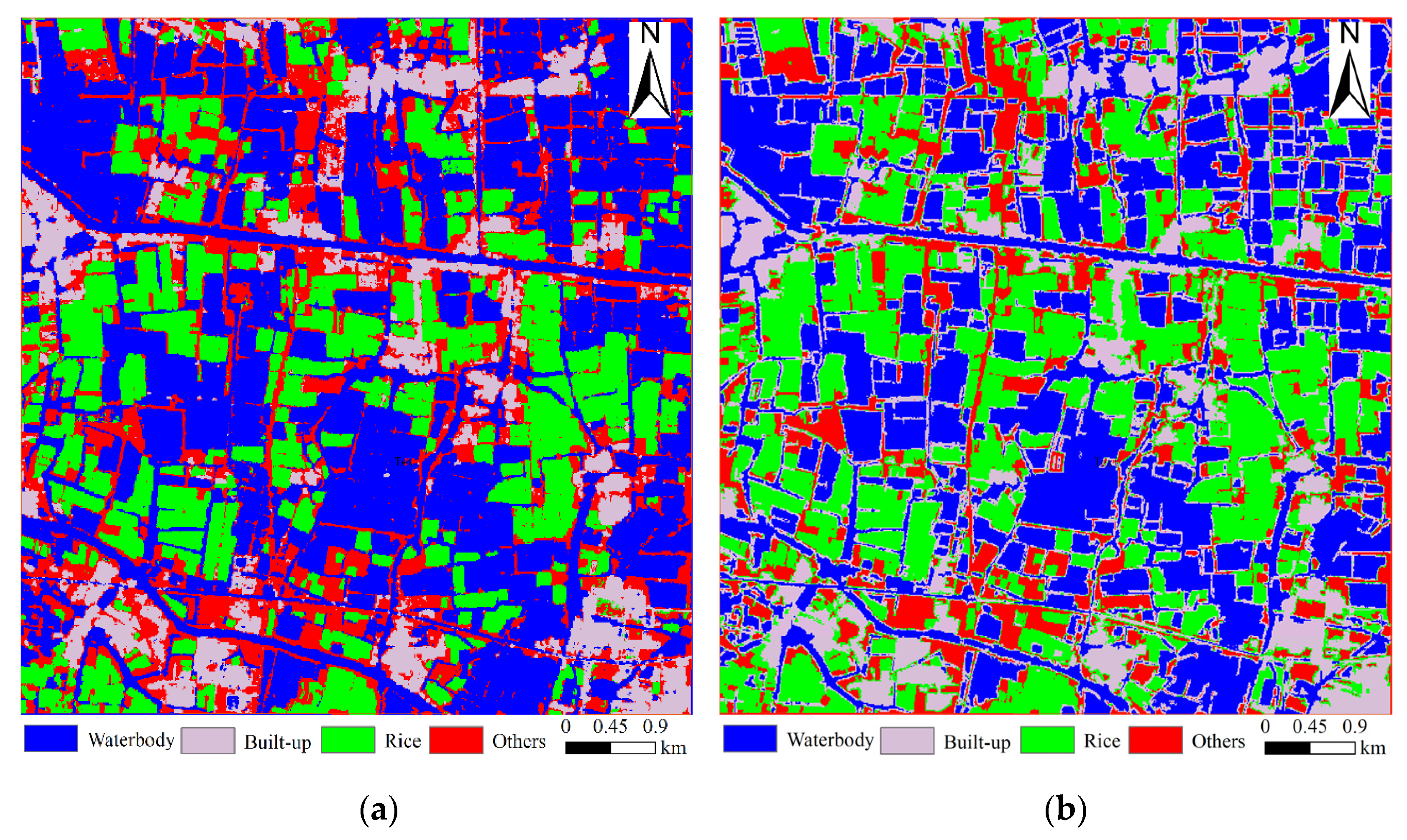
Besides, it can be found that compared with the pixel-based rice mapping, the PA of the superpixel-based classification has significantly improved, while the improvement of UA is quite small (Figure 9). It implies that rice mapping based on the SNIC method can significantly reduce the omission error of paddy rice. This is mainly due to the fact that the superpixel is obtained based on the high-resolution GF-1 pan-sharpened image, which can produce more accurate field boundaries and is not easy to omit small fields (Figure 10).
6. Conclusions
A 2 m resolution GF-1 pan-sharpened image was segmented into superpixels based on the SNIC algorithm and then used for rice mapping based on time-series Sentinel-2 MSI optical images and Sentinel-1 C-SAR images. Several key conclusions were drawn as follows:
- The value of the superpixel size has a significant influence on the classification accuracy of SNIC based high-resolution image classification.
- The combination of optical and SAR images can increase the classification accuracy of superpixel-based rice mapping compared with using only optical or SAR images.
- Superpixel-based classification based on SNIC method significantly outperforms the pixel-based classification for the five image combinations, especially when only using time-series Sentinel-1 SAR images.
In future research, the automatic optimal superpixel segmentation size selection method is still need to be developed to improve the classification efficiency and accuracy. Meanwhile, the large-scale crop mapping based on SNIC segmentation of high-resolution images still needs to be focused on.
Author Contributions
Conceptualization, L.Y., L.W., G.A.A. and J.H.; methodology, L.Y. and G.A.A.; software, L.Y.; validation, L.Y.; formal analysis, L.Y., G.A.A. and J.H.; investigation, L.Y.; resources, L.Y. and L.W.; data curation, L.Y.; writing—original draft preparation, L.Y., G.A.A.; writing—review and editing, L.Y., G.A.A.; visualization, L.Y.; supervision, J.H.; project administration, J.H.; funding acquisition, J.H. and L.W. All authors have read and agreed to the published version of the manuscript.
Funding
This research was funded by National Major Project of China, grant number 09-Y20A05-9001-17/18 and Eramus+ Programme of the European Union, grant number 598838-EPP-1-2018-EL-EPPKA2-CBHE-JP.
Institutional Review Board Statement
Not applicable.
Informed Consent Statement
Not applicable.
Data Availability Statement
The data presented in this study are available on request from the corresponding author.
Acknowledgments
We thank Weiwei Liu, Ruzimaimaiti Mijiti, Yan Chen, and Wenjie Li of the Key Laboratory of Agricultural Remote Sensing and Information Systems of Zhejiang University, for their help in ground data collection. We also thank the anonymous reviewers for their constructive comments and advice.
Conflicts of Interest
The authors declare no conflict of interest.
References
- Wu, M.; Huang, W.; Niu, Z.; Wang, Y.; Wang, C.; Li, W.; Hao, P.; Yu, B. Fine crop mapping by combining high spectral and high spatial resolution remote sensing data in complex heterogeneous areas. Comput. Electron. Agric. 2017, 139, 1–9. [Google Scholar] [CrossRef]
- Ozdarici-Ok, A.; Ok, A.O.; Schindler, K. Mapping of agricultural crops from single high-resolution multispectral images—Data-driven smoothing vs. parcel-based smoothing. Remote Sens. 2015, 7, 5611–5638. [Google Scholar] [CrossRef] [Green Version]
- Yang, L.; Wang, L.; Huang, J.; Mansaray, L.R.; Mijiti, R. Monitoring policy-driven crop area adjustments in northeast China using Landsat-8 imagery. Int. J. Appl. Earth Obs. 2019, 82, 101892. [Google Scholar] [CrossRef]
- Zhou, Q.; Yu, Q.; Liu, J.; Wu, W.; Tang, H. Perspective of Chinese GF-1 high-resolution satellite data in agricultural remote sensing monitoring. J. Integr. Agr. 2017, 16, 242–251. [Google Scholar] [CrossRef]
- Lv, Z.; Shi, W.; Zhang, X.; Benediktsson, J.A. Landslide inventory mapping from bitemporal high-resolution remote sensing images using change detection and multiscale segmentation. IEEE J. Sel. Top. Appl. Earth Obs. Remote Sens. 2018, 11, 1520–1532. [Google Scholar] [CrossRef]
- Mansaray, L.R.; Yang, L.; Kabba, V.T.; Kanu, A.S.; Huang, J.; Wang, F. Optimising rice mapping in cloud-prone environments by combining quad-source optical with Sentinel-1A microwave satellite imagery. Gisci. Remote Sens. 2019, 56, 1333–1354. [Google Scholar] [CrossRef]
- Erinjery, J.J.; Singh, M.; Kent, R. Mapping and assessment of vegetation types in the tropical rainforests of the Western Ghats using multispectral Sentinel-2 and SAR Sentinel-1 satellite imagery. Remote Sens. Environ. 2018, 216, 345–354. [Google Scholar] [CrossRef]
- Fu, B.; Wang, Y.; Campbell, A.; Li, Y.; Zhang, B.; Yin, S.; Xing, Z.; Jin, X. Comparison of object-based and pixel-based Random Forest algorithm for wetland vegetation mapping using high spatial resolution GF-1 and SAR data. Ecol. Indic. 2017, 73, 105–117. [Google Scholar] [CrossRef]
- Yang, L.; Mansaray, L.R.; Huang, J.; Wang, L. Optimal Segmentation Scale Parameter, Feature Subset and Classification Algorithm for Geographic Object-Based Crop Recognition Using Multisource Satellite Imagery. Remote Sens. 2019, 11, 514. [Google Scholar] [CrossRef] [Green Version]
- Makinde, E.O.; Salami, A.T.; Olaleye, J.B.; Okewusi, O.C. Object Based and Pixel Based Classification Using Rapideye Satellite Imager of ETI-OSA, Lagos, Nigeria. Geoinformatics FCE CTU 2016, 15, 59–70. [Google Scholar] [CrossRef]
- Csillik, O. Fast segmentation and classification of very high resolution remote sensing data using SLIC superpixels. Remote Sens. 2017, 9, 243. [Google Scholar] [CrossRef] [Green Version]
- Gong, Y.; Zhou, Y. Differential evolutionary superpixel segmentation. IEEE Trans. Image Process. 2017, 27, 1390–1404. [Google Scholar] [CrossRef]
- Duro, D.C.; Franklin, S.E.; Dubé, M.G. A comparison of pixel-based and object-based image analysis with selected machine learning algorithms for the classification of agricultural landscapes using SPOT-5 HRG imagery. Remote Sens. Environ. 2012, 118, 259–272. [Google Scholar] [CrossRef]
- Ma, L.; Cheng, L.; Li, M.; Liu, Y.; Ma, X. Training set size, scale, and features in Geographic Object-Based Image Analysis of very high resolution unmanned aerial vehicle imagery. ISPRS J. Photogramm. 2015, 102, 14–27. [Google Scholar] [CrossRef]
- Graesser, J.; Ramankutty, N. Detection of cropland field parcels from Landsat imagery. Remote Sens. Environ. 2017, 201, 165–180. [Google Scholar] [CrossRef] [Green Version]
- Waldner, F.; Diakogiannis, F.I. Deep learning on edge: Extracting field boundaries from satellite images with a convolutional neural network. Remote Sens. Environ. 2020, 245, 111741. [Google Scholar] [CrossRef]
- Achanta, R.; Susstrunk, S. Superpixels and polygons using simple non-iterative clustering. In Proceedings of the IEEE Conference on Computer Vision and Pattern Recognition, Honolulu, HI, USA, 21–26 July 2017; pp. 4651–4660. [Google Scholar]
- Schultz, B.; Immitzer, M.; Formaggio, A.R.; Sanches, I.D.A.; Luiz, A.J.B.; Atzberger, C. Self-guided segmentation and classification of multi-temporal Landsat 8 images for crop type mapping in Southeastern Brazil. Remote Sens. 2015, 7, 14482–14508. [Google Scholar] [CrossRef] [Green Version]
- Xu, Q.; Fu, P.; Sun, Q.; Wang, T. A Fast Region Growing Based Superpixel Segmentation for Hyperspectral Image Classification. In Proceedings of the Chinese Conference on Pattern Recognition and Computer Vision (PRCV), Xi’an, China, 8–11 November 2019; Springer: Cham, Switzerland, 2019; pp. 772–782. [Google Scholar]
- Paludo, A.; Becker, W.R.; Richetti, J.; Silva, L.C.D.A.; Johann, J.A. Mapping summer soybean and corn with remote sensing on Google Earth Engine cloud computing in Parana state–Brazil. Int. J. Digit. Earth. 2020, 13, 1624–2636. [Google Scholar] [CrossRef]
- Brinkhoff, J.; Vardanega, J.; Robson, A.J. Land Cover Classification of Nine Perennial Crops Using Sentinel-1 and-2 Data. Remote Sens. 2020, 12, 96. [Google Scholar] [CrossRef] [Green Version]
- Tassi, A.; Vizzari, M. Object-Oriented LULC Classification in Google Earth Engine Combining SNIC, GLCM, and Machine Learning Algorithms. Remote Sens. 2020, 12, 3776. [Google Scholar] [CrossRef]
- Tu, Y.; Chen, B.; Zhang, T.; Xu, B. Regional Mapping of Essential Urban Land Use Categories in China: A Segmentation-Based Approach. Remote Sens. 2020, 12, 1058. [Google Scholar] [CrossRef] [Green Version]
- Jia, S.; Zhan, Z.; Zhang, M.; Xu, M.; Huang, Q.; Zhou, J.; Jia, X. Multiple Feature-Based Superpixel-Level Decision Fusion for Hyperspectral and LiDAR Data Classification. IEEE Trans. Geosci. Remote Sens. 2020, 99, 1–19. [Google Scholar]
- Amani, M.; Mahdavi, S.; Afshar, M.; Brisco, B.; Huang, W.; Mohammad Javad Mirzadeh, S.; White, L.; Banks, S.; Montgomery, J.; Hopkinson, C. Canadian wetland inventory using Google Earth engine: The first map and preliminary results. Remote Sens. 2019, 11, 842. [Google Scholar] [CrossRef] [Green Version]
- Zhang, X.; Wu, B.; Ponce-Campos, G.E.; Zhang, M.; Chang, S.; Tian, F. Mapping up-to-date paddy rice extent at 10 m resolution in China through the integration of optical and synthetic aperture radar images. Remote Sens. 2018, 10, 1200. [Google Scholar] [CrossRef] [Green Version]
- Liu, J.; Wang, L.; Yang, L.; Shao, J.; Teng, F.; Yang, F.; Fu, C. Geometric correction of GF-1 satellite images based on block adjustment of rational polynomial model. Trans. Chin. Soc. Agric. Eng. 2015, 31, 146–154. [Google Scholar]
- Meng, X.; Shen, H.; Li, H.; Zhang, L.; Fu, R. Review of the pansharpening methods for remote sensing images based on the idea of meta-analysis: Practical discussion and challenges. Inform. Fusion. 2019, 46, 102–113. [Google Scholar] [CrossRef]
- Sarp, G. Spectral and spatial quality analysis of pan-sharpening algorithms: A case study in Istanbul. Eur. J. Remote Sens. 2014, 47, 19–28. [Google Scholar] [CrossRef] [Green Version]
- Congalton, R.G. A review of assessing the accuracy of classifications of remotely sensed data. Remote Sens. Environ. 1991, 37, 35–46. [Google Scholar] [CrossRef]
- Sharma, R.C.; Hara, K.; Tateishi, R. High-resolution vegetation mapping in japan by combining sentinel-2 and landsat 8 based multi-temporal datasets through machine learning and cross-validation approach. Land 2017, 6, 50. [Google Scholar] [CrossRef] [Green Version]
- Mi, L.; Chen, Z. Superpixel-enhanced deep neural forest for remote sensing image semantic segmentation. ISPRS J. Photogramm. 2020, 159, 140–152. [Google Scholar] [CrossRef]
- Breiman, L. Random forests. Mach. Learn. 2001, 45, 5–32. [Google Scholar] [CrossRef] [Green Version]
- Belgiu, M.; Csillik, O. Sentinel-2 cropland mapping using pixel-based and object-based time-weighted dynamic time warping analysis. Remote Sens. Environ. 2018, 204, 509–523. [Google Scholar] [CrossRef]
- Belgiu, M.; Drăguţ, L. Random forest in remote sensing: A review of applications and future directions. ISPRS J. Photogramm. 2016, 114, 24–31. [Google Scholar] [CrossRef]
- Zhan, P.; Zhu, W.; Li, N. An automated rice mapping method based on flooding signals in synthetic aperture radar time series. Remote Sens. Environ. 2021, 252, 112112. [Google Scholar] [CrossRef]
Figure 1.
Location of the study area: (a) Location of the study site; (b) GF-1 PMS false-color composite image of the study area.
Figure 1.
Location of the study area: (a) Location of the study site; (b) GF-1 PMS false-color composite image of the study area.

Figure 2.
Images on the bottom show the GF-1 multi-spectral (d), panchromatic (e) and pan-sharpened (f) images. Images on the top show their corresponding enlarged details (a–c).
Figure 2.
Images on the bottom show the GF-1 multi-spectral (d), panchromatic (e) and pan-sharpened (f) images. Images on the top show their corresponding enlarged details (a–c).

Figure 3.
Sentinel-2 MSI images in the study area on July (a), August (b), September (c), the first half of October (d), the second half of October (e), the first half of November (f), the second half of November (g) and the first ten days of December (h), 2017.
Figure 3.
Sentinel-2 MSI images in the study area on July (a), August (b), September (c), the first half of October (d), the second half of October (e), the first half of November (f), the second half of November (g) and the first ten days of December (h), 2017.

Figure 4.
Sentinel-1 C-SAR vertical transmitted and vertical received (VV) images in the study area on the first ten days of May (a), July (b), August (c), October (d), 2017, and VH images on the first ten days of the May (e), July (f), August (g) and October (h), 2017.
Figure 4.
Sentinel-1 C-SAR vertical transmitted and vertical received (VV) images in the study area on the first ten days of May (a), July (b), August (c), October (d), 2017, and VH images on the first ten days of the May (e), July (f), August (g) and October (h), 2017.

Figure 5.
Ground survey photos, including paddy rice field (a), seedling field (b), waterbody (c), and road (d).
Figure 5.
Ground survey photos, including paddy rice field (a), seedling field (b), waterbody (c), and road (d).


Figure 6.
Location map of random sample points and field campaigns.

Figure 7.
Methodological workflow employed in the current study.

Figure 8.
Overall, producer, and user accuracies of superpixel-based rice mapping. S2 represents rice mapping based on Sentinel-2 MSI images. VV represents rice mapping based on Sentinel-1 C-SAR VV images. VH represents rice mapping based on Sentinel-1 C-SAR VH images. VV + VH represents rice mapping based on Sentinel-1 C-SAR VV and VH images. S2 + VV + VH represents rice mapping based on Sentinel-2 MSI images, Sentinel-1 C-SAR VV, and VH images. (a) Overall accuracy; (b) Producer accuracy; (c) User accuracy.

Figure 9.
Classification accuracies of pixel-based classification and superpixel-based classification: (a) Overall accuracy; (b) Producer accuracy; (c) User accuracy.
Figure 9.
Classification accuracies of pixel-based classification and superpixel-based classification: (a) Overall accuracy; (b) Producer accuracy; (c) User accuracy.

Figure 10.
Results of pixel-based (a) and superpixel-based (b) classification based on S2 + VV + VH dataset.
Figure 10.
Results of pixel-based (a) and superpixel-based (b) classification based on S2 + VV + VH dataset.


Table 1.
Characteristics of the GF-1 panchromatic/multi-spectral data.
| Sensor | Band Name | Wavelength (μm) | Resolution (m) |
|---|---|---|---|
| Panchromatic | Panchromatic | 0.45–0.90 | 2 |
| Multi-spectral | Blue | 0.45–0.52 | 8 |
| Green | 0.52–0.59 | ||
| Red | 0.63–0.69 | ||
| Near infrared | 0.77–0.89 |
Table 2.
Characteristics of the Sentinel-2 Multispectral Instrument data.
| Band Name | Description | Wavelength (μm) | Resolution (m) |
|---|---|---|---|
| B1 | Aerosols | 0.4439 | 60 |
| B2 | Blue | 0.4966 | 10 |
| B3 | Green | 0.5600 | 10 |
| B4 | Red | 0.6645 | 10 |
| B5 | Red edge 1 | 0.7039 | 20 |
| B6 | Red edge 2 | 0.7402 | 20 |
| B7 | Red edge 3 | 0.7825 | 20 |
| B8 | Near infrared | 0.8351 | 10 |
| B8A | Red edge 4 | 0.8648 | 20 |
| B9 | Water vapor | 0.9450 | 60 |
| B10 | Cirrus | 1.3735 | 60 |
| B11 | Short-wave infrared 1 | 1.6137 | 20 |
| B12 | Short-wave infrared 2 | 2.2024 | 20 |
| QA | Cloud mask | - | 60 |
Table 3.
Classification schemes.
| SNIC | Superpixel Size | Image Combinations |
|---|---|---|
| GF-1 pan-sharpened image | 16–100 | Sentinel-2 MSI (S2) |
| Sentinel-1 C-SAR VV (VV) | ||
| Sentinel-1 C-SAR VH (VH) | ||
| Sentinel-1 C-SAR VV + VH (VV + VH) | ||
| Sentinel-1 C-SAR VV + VH + Sentinel-2 MSI (S2 + VV + VH) |
Publisher’s Note: MDPI stays neutral with regard to jurisdictional claims in published maps and institutional affiliations. |
© 2021 by the authors. Licensee MDPI, Basel, Switzerland. This article is an open access article distributed under the terms and conditions of the Creative Commons Attribution (CC BY) license (http://creativecommons.org/licenses/by/4.0/).
Share and Cite
MDPI and ACS Style
Yang, L.; Wang, L.; Abubakar, G.A.; Huang, J. High-Resolution Rice Mapping Based on SNIC Segmentation and Multi-Source Remote Sensing Images. Remote Sens. 2021, 13, 1148. https://doi.org/10.3390/rs13061148
AMA Style
Yang L, Wang L, Abubakar GA, Huang J. High-Resolution Rice Mapping Based on SNIC Segmentation and Multi-Source Remote Sensing Images. Remote Sensing. 2021; 13(6):1148. https://doi.org/10.3390/rs13061148
Chicago/Turabian StyleYang, Lingbo, Limin Wang, Ghali Abdullahi Abubakar, and Jingfeng Huang. 2021. "High-Resolution Rice Mapping Based on SNIC Segmentation and Multi-Source Remote Sensing Images" Remote Sensing 13, no. 6: 1148. https://doi.org/10.3390/rs13061148
Note that from the first issue of 2016, this journal uses article numbers instead of page numbers. See further details here.