
Cropmarks in Aerial Archaeology: New Lessons from an Old Story
by
 ,
,
Zoltán Czajlik
1,*, 
Mátyás Árvai
2,
János Mészáros
2 ,
,
Balázs Nagy
3,
László Rupnik
4 and
László Pásztor
2 1
Department of Archeometry, Archaeological Heritage and Methodology, Institute of Archaeological Sciences, Faculty of Humanities, Eötvös Loránd University, Múzeum krt. 4/B, 1088 Budapest, Hungary
2
Institute for Soil Sciences, Centre for Agricultural Research, Herman Ottó út 15, 1022 Budapest, Hungary
3
Department of Physical Geography, Center of Geography, Faculty of Science, Eötvös Loránd University, Pázmány Péter sétány 1, 1117 Budapest, Hungary
4
MTA-ELTE Research Group for Interdisciplinary Archaeology, Múzeum krt. 4/B, 1088 Budapest, Hungary
*
Author to whom correspondence should be addressed.
Remote Sens. 2021, 13(6), 1126; https://doi.org/10.3390/rs13061126
Submission received: 31 December 2020
/
Revised: 25 February 2021
/
Accepted: 9 March 2021
/
Published: 16 March 2021
(This article belongs to the Special Issue Archaeological Remote Sensing in the 21st Century: (Re)Defining Practice and Theory)
Abstract
:Cropmarks are a major factor in the effectiveness of traditional aerial archaeology. Identified almost 100 years ago, the positive and negative features shown by cropmarks are now well understood, as are the role of the different cultivated plants and the importance of precipitation and other elements of the physical environment. Generations of aerial archaeologists are in possession of empirical knowledge, allowing them to find as many cropmarks as possible every year. However, the essential analyses belong mostly to the predigital period, while the significant growth of datasets in the last 30 years could open a new chapter. This is especially true in the case of Hungary, as scholars believe it to be one of the most promising cropmark areas in Europe. The characteristics of soil formed of Late Quaternary alluvial sediments are intimately connected to the young geological/geomorphological background. The predictive soil maps elaborated within the framework of renewed data on Hungarian soil spatial infrastructure use legacy, together with recent remote sensing imagery. Based on the results from three study areas investigated, analyses using statistical methods (the Kolmogorov–Smirnov and Random Forest tests) showed a different relative predominance of pedological variables in each study area. The geomorphological differences between the study areas explain these variations satisfactorily.
1. Introduction
In June 1998, one of the most prolific aerial archaeologists of the second half of the 20th century, René Goguey, arrived in Budapest from Paris on an Air France scheduled flight. While still at the airport, he commented that from an altitude of 20,000 feet it was clear to him that research into cropmarks on the Little Plain (Rába interfluve) should begin immediately. Despite the previous several years’ lack of success, work was recommenced in this region, and a large number of good quality archaeological features visible as cropmarks were identified [1].
To understand the significance and the complexity of cropmarks in aerial archaeology, a brief summary of traditional ways of investigating them and a short presentation of the factors affecting their formation are required. Alluvial fans are ideal for studying the role of the different soils in the formation of cropmarks, and therefore, this introduction will also contain the geographical background of the alluvial fans and the relevant results of soil mapping in Hungary.
1.1. Cropmarks in Aerial Archaeology
What has been long recognized is the correlation between variations in vegetation on arable land (and, under certain conditions, on grazed and mowed areas) and the presence of traces of past human activities (along with many natural phenomena). Although there were indications of an understanding that vegetation might reveal the past in this way as early as around 1540 (John Leland), it was the work of O. G. S. Crawford in the UK beginning in 1914 that definitively linked variations in crop growth to the presence of buried archaeological features [2]. By the 1920s, this was already being applied in his research [3]. The development of aviation and aerial photography then led to similar insights in continental Europe, too. In Hungary, Sándor Neogrády, another experienced World War I aviator, was an aerial photographer and cartographer who started to collect what he termed “unnatural phenomena” from the 1920s [4]. Pioneer researchers began to organize them systematically, so Neogrády also described the role of darker, denser vegetation, which grows over filled-in ditches/pits, and the sparser, lighter vegetation over buried walls, introducing the distinction between positive and negative cropmarks as basic categories [4].
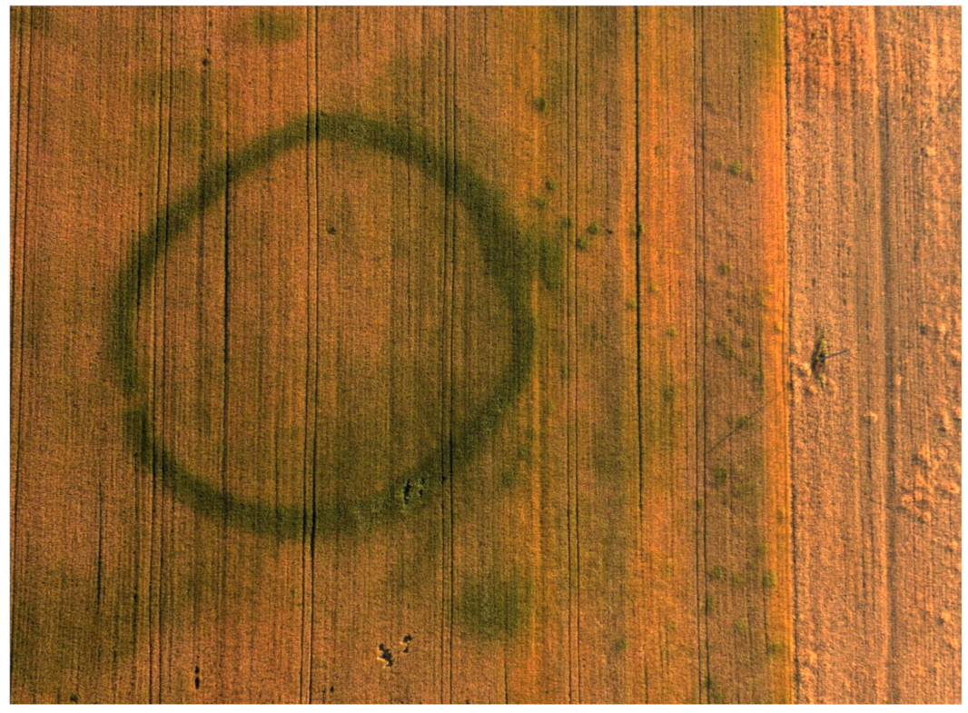
In addition to variations in color, differences in the height of crops and vegetation are also important (Figure 1), as illustrated in various studies [5,6]. Many cultivated plant species indicate anomalies very early in their growing season, but it is in the course of ripening that the greater part of variations may be detected [7,8].
From the 1950s, first in France and Germany, later in Austria and Italy, and finally in the 1990s in Switzerland and the former socialist countries, the importance assigned to the identification of the cropmarks has grown. This, together with data gathered using traditional, analog aerial photography in archaeology, was summarized by Irwin Scollar in his work on archaeological prospection, which is still relevant today [9].
Beginning in the 2000s, the use of digital cameras and GPS for positioning images and navigation has greatly increased the efficiency of traditional aerial archaeological data collection. Images with reference points can be quickly rectified, and the interpretation and creation of photomaps has become much easier. Thanks to digital technology, it is now possible to collect information not only from the visible spectrum, but also from the NIR and NUV domains, which (in a way similar to infrared films in the analog era) can increase the contrast between normal and stressed crops and improve the visibility of cropmarks following data enhancement [10].
Nowadays, archaeological aerial photography has become part of airborne and space-borne remote sensing (ASRS), in addition to those mentioned above, as well as the multi- and hyperspectral applications [11]. The programmed use of the latest UAV platform—as with non-traditional ASRS—makes (semi) automatic photography also possible. Thus, traditional aerial archaeology remains one of the last remote sensing techniques requiring an observer, so its overhaul is certainly justified [12,13]. However, this does not lead to the undervaluing or discarding of the experience and benefits that come from the observer being not only part of the learning process, but also being constantly present during data collection and influencing its quality and efficiency through decisions; all this represents a resource to be exploited. This is especially true in the case of such a complex phenomenon as cropmarks, which are to this day still understood on the basis, more or less, of empirical knowledge [14].
1.2. Factors Affecting the Formation of Cropmarks
As summarized above, the experiences of pioneers in this field show that what character and what quality of cropmarks become visible depends on when a photo is taken. Some of these factors are connected to agricultural activity: in which way the soil is cultivated, and above all, what species are grown, and in what proportion [15]. The significance of barley (Hordeum vulgare), wheat (Triticum aestivum), winter rape (Brassica napus) and alfalfa (Medicago sativa) in this area of research is well-documented. To varying degrees, maize (Zea mays L.), pea (Pisum sativum L.) and sun-flower (Helianthus annuus L.) may also reveal archaeological features [16]. On the basis of the personal experience of the authors of the present paper, triticale (Triticale) and poppy (Papaver somniferum L.) also have important regional roles [17]. The explanation for these observations is mainly related to the sowing distance, structure (e.g., normal root length) and drought tolerance/resistance to high amounts of precipitation of the plants [18,19].
One of the most difficult natural factors to calculate is the weather, and the personal experience of both the aerial photographer‒archaeologist and the pilot still plays an important role in dealing with this. As a general rule, droughts caused by dry weather can dramatically increase the number of detectable cropmarks, which is what happened in England in 1976. Too much rainfall, on the other hand, yields few cropmarks, while a lot of rain in early summer can ruin even what had earlier been regarded as promising cropmark development—this is what happened in Hungary in 2019, for example.
Taking all the above into account, the investigation of the correlation between infiltration/evaporation data and cropmarks requires the detailed analysis not only of data sets for late spring/early summer but also of long-term sets [20,21,22,23]. Furthermore, it should be noted here that while the analysis of precipitation-related factors is important, it is not in itself sufficient; temperature and even, in some cases wind, may also be of significance [24].
Among the geological factors, the role of gravel-rich subsurface layers or gravel covers and fluvial-dominated fan surfaces is of extraordinary importance [25,26]. On the basis of data from Bavaria, it would appear that even in moderately rainy years, good results can be achieved by researching these areas [5]. In Central Bohemia, in the Elbe Basin, 75% of the cropmarks identified between 1993 and 2009 are in gravel/sandy areas, and a further 22% in territories underlain by loess bedrock [16]. Such areas can be successfully investigated in Hungary as well, though in this case, the difference in favor of gravel/sand areas is not as remarkable [17,23].
While soil conditions are, naturally, not independent of the underlying geology, alluvial areas may, nonetheless, present a very diverse picture, making it difficult to recognize correlations with soil types. The effects of sub-soil archaeological features on the growth of crops and the related question of within-plot variability in soil properties has been studied in Central European agricultural landscapes by Czech researchers. Hejcman et al. (2013) [27] were able to demonstrate that variations in soil pH and nutrient availability were attributable to prehistoric settlement activities. They recorded substantially higher contents of organic matter, higher pH, and concentrations of plant-available P, Ca, Mg, Cu, and Zn in the sub-soil layer in cropmarks identified on spring barley as compared to their surroundings. In the arable layer, pH and concentrations of P, Ca and Mg were generally higher. Cropmarks were characterized by barley plants that grew to twice the height of those in the control group, and with significantly higher Ca, Mg and P concentrations. In Bohemia, the cropmarks were most visible on sandy soils, as the soil texture, water holding capacity, and nutrient availability between filled-in archaeological features and the surrounding sub-soil layers showed the greatest contrast. The soil properties differ significantly in areas with clayey soils, which may explain the almost complete absence of cropmarks in these zones [16,28,29]. According to Gojda and Hejcman, positive cropmarks may appear particularly noticeable above graves due to the phosphorus from the bodies [19]. On the basis of the experiences of the current authors, it should be noted that the identification of graves through cropmarks is more sensitive to weather/precipitation than is the case with other archaeological phenomena.
1.3. Geographical Background
The interior of the Carpathian Basin is dominated by lowlands derived from alluvial fans. The watercourses reaching the basin from the mountainous surroundings formed their vast alluvial fans with lengths of 10 km to 100 km, stretching out towards the deep-lying part of the giant basin during the Pleistocene [30]. The alluvial fans—representing a total area of more than 50,000 km2—are separated by low mountains and gentle hills. Elsewhere, however, interlinked alluvial fans underwent significantly different Late Pleistocene and Holocene development histories; in these cases, due to both tectonic and climatic processes, the watercourses gradually “slid down” (migrated) from the alluvial fans with gravel bases and silty and sandy sediment dominated upper layers [31].
On some of the alluvial fans—e.g., on the remnants of an alluvial fan flanked by a terraced valley edge—the movements of wind-blown sand and loess formation became dominant. The sand-formed topography is dominated by large blowout-residual ridge-hummock form assemblages that are extensive and adapt to the runoff direction(s) of the former alluvial fan surface.
In other cases, the tectonic fragmentation of former alluvial fans with thick loess and sand cover formed a tectonically controlled valley network. Their streams sharply divided the alluvial fan bodies: alluvial valleys were formed, with steep marginal slopes, above which extended flat plateaus with a geological past as alluvial fans but subsequently were covered with loess and/or sand.
At the edges of the alluvial fans, the rivers that migrated there formed wide floodplains. After their strong alluvial fan erosion activity, during the accumulation phase-which is also characteristic of the Holocene—they partially covered the marginal areas with their sediments, or they could even cover the entire surface of the smaller alluvial fan.
1.4. Soil Mapping
The upper, weathered, solid mantle of the Earth, the pedosphere, results from the complex interplay of several soil forming factors and soil forming processes in the zone of interaction between the lithosphere, atmosphere, hydrosphere and biosphere. Soil is a multifunctional natural resource [32], one of its main functions is the conservation of natural and human heritages.
The goal of soil mapping is to reveal and visualize the spatial relationships of thematic knowledge concerning the soil mantle. Soil maps are thematic maps, whereby a theme is determined through specific information related to the soils [33]. These can be primary or secondary (derived), quantitative, or qualitative properties. There are two basic and apparently contradictory but in fact complementary concepts employed in the characterization of spatial variability in soils [34]. One approach essentially builds on similarity, and represents the soil mantle via the mapping of units of homogeneous composition. Its cartographic realization is classic soil maps, of which there is an extensive tradition [34]. The other approach emphasizes the continuous spatial variation of soil properties, and the mapped soil property is predicted using cells and the spatial resolution is determined by the cell size.
In Hungary, large amounts of soil information have been collected through soil surveys, observation and mapping. The goals and methodology of successive soil mapping projects differed, and as a consequence, very often it was dissimilar soil features that were highlighted. The maps were compiled at various scales, from farm to national level. Smaller scale, synthesized maps provide national coverage, while larger scale ones cover only parts of the country [35].
Recently, predictive soil maps in the form of digital soil maps have come to be considered the most effective representation of specific features of the soil mantle [36]. The evolution of digital soil mapping is closely related to the rising availability of spatially exhaustive, relatively low-cost data available in the form of satellite imagery covering wide time scales and spectra, and also digital elevation models originating from remote sensing, both of which provide efficient representations of various soil forming factors and processes [37]. In Hungary, the very recently elaborated DOSoReMI.hu is a collection of spatial soil information in the form of unique digital soil map products compiled to optimize the identification of specific soil features at the regional scale [38]. A significant part of these had never been mapped before, even nationally, at a high (~1 ha) spatial resolution. The new digital soil maps are compiled from specific spatial predictions based on (i) measured soil observation data, (ii) spatially exhaustive, environmental auxiliary variables, and (iii) sophisticated geostatistical and data mining methods for inferring the spatial and temporal variations of soil features. The inherent vagueness of spatial prediction is explicitly expressed through a proper accuracy assessment, and the newly produced digital soil information and maps are therefore supplied with an estimation of the degree of both local and global uncertainty or reliability.
2. Materials and Methods
Studying cropmarks requires a special mixture of knowledge, as besides the technical factors, its efficiency depends on experience of the local setting, archaeological and geomorphological knowledge, and on environmental factors which are permanently changing with respect to one another. Among these dynamic factors, the role of precipitation is decisive, and the weather during the early summer time window can influence the results for better or for worse to a great extent. In the light of this, it is clear why methods may vary greatly in heritage management, but the greater the researcher’s experience and the longer the research timescale, the greater the progress which can be made in reducing the impact of seasonal differences.
The primary spatial unit of the traditional archaeological approach is the archeological site. Official geoinformatics-based records rely on the sites being some kind of polygon clearly delimited in an area using field survey data. In the case of aerial archaeological sites, the greater part of the data concerns the archaeological features. This allows a much more detailed interpretation than the information from a field survey. Thanks to the detailed interpretation of aerial photos, defining the archaeological site boundaries is not necessary [39]. However, in aerial archaeology research, sites can be defined as territorial units reshaped by the imposition of modern borders, divisions, and changes in designation and use. Nevertheless, the density of aerial archaeological sites are usually marked on integrated maps with the help of simple coordinates/GPS tracks determined during flights or later in laboratory, meaning that there is no spatial data showing their true extent in most databases [8,17,40,41,42]. One important exception is the system operated by the University of Vienna for years, as they use both coordinates and polygons [26,29]. The method—in some aspects similar to the Austrian one—employed by the current authors is, with a few exceptions, adapted to the growth of cultivated field crops. In the presentation it is not aerial photograph coordinates which are used, but polygons. Aerial photo polygons do not show the boundaries of archaeological sites, but the plots planted with the same species, and any archaeological phenomena thus revealed. So, these are units which, thanks to the presence of homogenous conditions, theoretically all the important archeological phenomena should be visible.
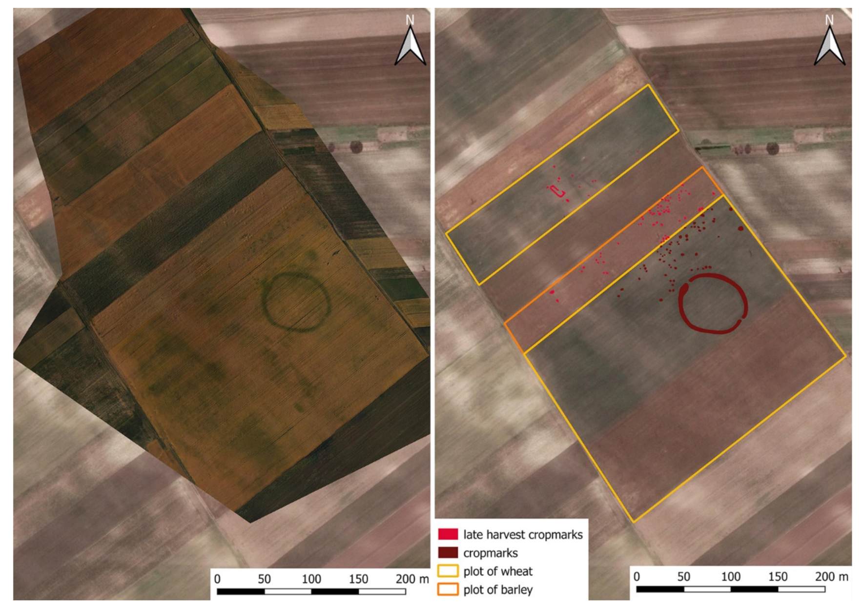
Herein, the term cropmark plot (CMP) will be used for the areas covered by each polygon. In the absence of CMPs, the extent of all archaeological aerial photo sites should be determined in order to obtain comparable spatial data. Meanwhile, there may be often several, in some cases even 8–10 aerially identifiable archaeological sites within the area of a CMP (Figure 2).
The opposite is, of course, also true. Maps of various archaeological sites can be put together, just like pieces of a puzzle, based on aerial archaeological prospection conducted on different dates. In other words, the number of puzzle pieces—and the average size of the CMPs—depends on the pattern of land use. To meet these conditions, the CMPs are formed on the basis of the polygons determined by the parcel boundaries at the time when the photo is taken. As a result of further photography, CMPs can be merged or resized if the documented area expands.
The aim of the current research was to compare the pedological features of cropmark plots (CMP) and non-cropmark plots (nCMP) in order to identify demonstrable differences between them. For this purpose, the spatial soil information on primary soil properties provided by DOSoReMI.hu was employed. To compensate for the inherent vagueness of spatial predictions, together with the fact that the definition of CMPs and nCMPs adopted here is somewhat indefinite, the comparisons were carried out using data-driven, statistical approaches.
2.1. Study Areas
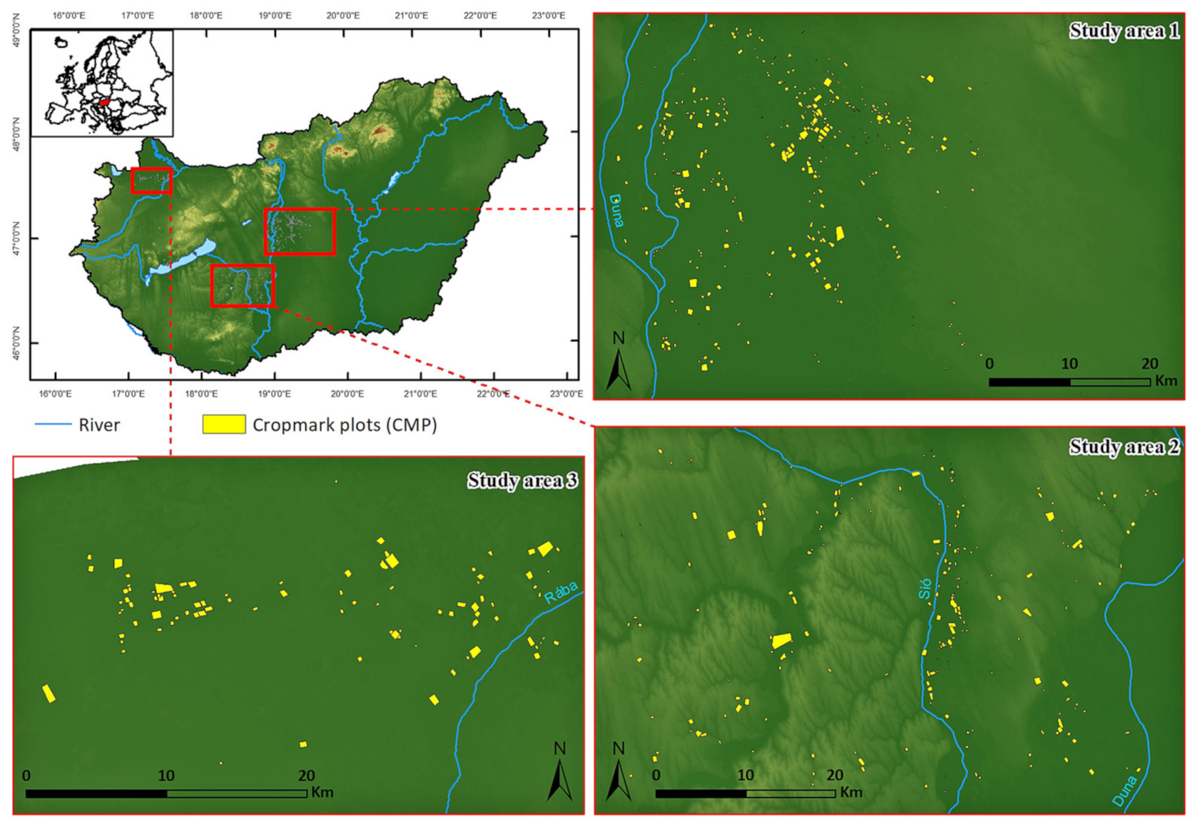
To examine the utility of this method, areas subject to increased systematic research from 1993 onwards were selected, and 2017 was the last year processed. This does not, however, mean that the regular aerial archaeological prospecting of the areas has ceased. The sample areas also represent examples of all three characteristic alluvial fan evolution types (1, 2, 3). These distinct environment types also demonstrate different patterns in terms of cropmark appearance (Figure 3).
- The alluvial fan of the Danube-Tisza interfluve (Study area 1)
This is a remnant of a huge alluvial fan of the paleo-Danube aligned in a NW-SE direction, and from which the river—for tectonic reasons—migrated to the West. In this new location, the Danube has created a wide floodplain extending 30–50 m below the top of the former alluvial fan. On the surface of the inactive alluvial fan there is a gravel-rich alluvial plain in the North but going southwards it is dominated by loess and sandy sediments, and due to aeolian processes (which were extremely significant in the Holocene as well), by sand ridges, hollows and dunes. A near-surface gravel presence occurs at the neck of the alluvial fan and on the terraces of the Danube as it cuts into its western margin.
- 2
- Sió-Sárvíz valley (Study area 2)
The Carpathian Basin has been divided by fluvial activity (the paleo-Danube) and controlled by tectonic processes. This loess and sand region is markedly separated from the wide floodplain of the Danube due to its Pleistocene migration and even from the sandy surface of the wide alluvial fan of the Danube-Tisza interfluve. In the Sió-Sárvíz valley, which deepens into a tectonically divided terrain, significant valley widening and slope erosion took place. The area’s classification as a lowland can be explained by the flat surface of the extensive loess and sandy plateaus that dominate the region.
- 3
- Rába interfluve (Study area 3)
The alluvial fans of the section of the paleo-Danube entering the Carpathian Basin and of the watercourses (e.g., Rába) coming from the eastern edge of the Alps developed into one of the sub-basins of the Carpathian Basin-in the direction of the Győr Basin. The gravel-dominated alluvial fans were built on top of each other in this lowland depression. Their floodplain sedimentary cover also significantly thickened during the Holocene, covering the alluvial fan-derived basement.
All the three study areas were preprocessed for the analysis in four steps:
- A minimum bounding box was defined, covering the CMPs of the given site. Its extent is defined by the outermost CMPs. The distribution of CMPs within these rectangles is inhomogeneous.
- The countrywide soil property maps with 1 ha spatial resolution were clipped to the extent of the bounding rectangles.
- Non-croplands were masked out from the clipped soil property maps on the basis of the very recently elaborated, national, high resolution ecosystem-type map [43], which also represents land-use/landcover characteristics with a high degree of accuracy.
- Two sample populations were defined for each test site and each soil property, containing (1) the raster cells in CMPs and (2) the rest of the cells. These sample populations represented the two types of areas, which show cropmark features, or not, respectively.
2.2. Spatial Soil Information
Traditionally, the spatial knowledge of soils is summarized chiefly in the form of soil type maps based on an appropriate classification system [44]. Generally, these maps are simply called soil maps, which in fact reflects their importance. Historically, soil mapping was done based on soil typology, and soil types have strong didactic significance. Soil type maps have also been created on different levels and according to different classification systems. In present study, the cartographically prepared (raster-vector transformed and generalized) version of the newly compiled nationwide soil type map (with harmonized legend and spatially consistent predictivity [45], was used for the identification of the location of CMPs along main soil types.
In the quantitative investigations, optimized primary soil property maps with 1 ha spatial resolution were tested for their ability to reveal differences between CMPs and nCMPs. As with soil type, rooting depth refers to the whole soil profile (pedon), while particle size fractions (clay, sand and silt content), bulk density (BD), soil organic matter content (SOM), CaCO3 content (CC), and pH are mapped for subsequent soil layers according to various partitions (Table 1). Each target variable was modelled using a sequence of spatial inference approaches (altering either methods or the reference and predictor data), which were always accompanied by a detailed accuracy assessment for the determination of the best performing set of soil data, method and auxiliary covariables for the given target variable [38]. The map products are published on the www.dosoremi.hu website and are serviced in two different ways. The maps elaborated according to GSM specifications represent the Hungarian contribution to the GlobalSoilMap.net project.
2.3. Statistical Methods
To identify their pedological differences, the two types of area underwent (i) testing using a traditional, non-parametric statistical test, namely the Kolmogorov–Smirnov (KS) homogeneity test and (ii) modelling using a recently “popularized” data mining method, namely Random Forest (RF). Despite their inherent differences, both methods are appropriate for revealing the hypothesized differences in the two types of areas on the basis of the available data.
2.3.1. Kolmogorov–Smirnov Homogeneity Test
The two-sample Kolmogorov–Smirnov (KS) homogeneity test is used to test whether two samples come from the same distribution by comparing the cumulative distributions of the two data sets. A great advantage of this non-parametric test is that it does not assume that data are sampled from normal distributions. The null hypothesis is that both groups were sampled from populations with identical distributions. The KS test reports the maximum difference (D) between the two cumulative distributions and calculates a p value from that and the sample sizes. The p value shows what the chances are that the value of the Kolmogorov–Smirnov D statistic is as large, or larger than observed. If the p value is small, the two groups are sampled from populations with different distributions.
The distribution of raster values for the two sample populations was compared by KS for each soil property independently for the three pilot areas. The two distributions were considered statistically different at a 95% confidence level, then the soil properties with P < 0.05 were ranked according to their D values. The higher the D value, the greater degree to which CMPs and nCMPs differ in their tested soil property.
2.3.2. Random Forests
Random Forests (RF) are an ensemble data mining method for classification and/or regression. The RF algorithm depending on its settings and on the type of the dependent variable, generates a number of regression or classification trees. The model relies on averaging the result of the trees, which are grown independently of each other [46]. In the course of RF modelling, the number of trees was set at 500, the number of variables available for splitting at each tree node (mtry) was set at 7 (501/2). RF models provide a variable rank, reflecting which co-variables play a more important role in the prediction model. According Hengl et al. (2017) [47], the main advantages of random forest over linear regression are: (i) it has no requirements in terms of the probability distribution of the target variable; (ii) it can fit complex non-liner relationships in k+1-dimensional space (where k is the number of environmental covariates); and (iii) the correlation between the environmental covariates is not a limiting factor.
In the present study, the prediction of CMPs and nCMPs was tested using RF modelling. The test dataset was set up by using all raster values for each study areas, and a binary classification was carried out for the identification of CMPs and nCMPs. The variable degrees of importance provided by RF were used for the ranking of soil properties in the discrimination. RF was carried out once on genetic soil type and once only with merely quantitative predictors.
3. Results
Differences in geological/geomorphological background alone do not explain all anomalies. It was presumed that the recent state of soil formation, expressed by genetic soil type, water absorption and water holding as well as nutrition supply capacity, would play an essential role, too.
3.1. Distribution of CMPs along Main Genetic Soil Types
As witnessed in the study areas, Chernozem and Meadow type soils are remarkably helpful in the formation of cropmarks, while the suitability of sandy soils is limited.
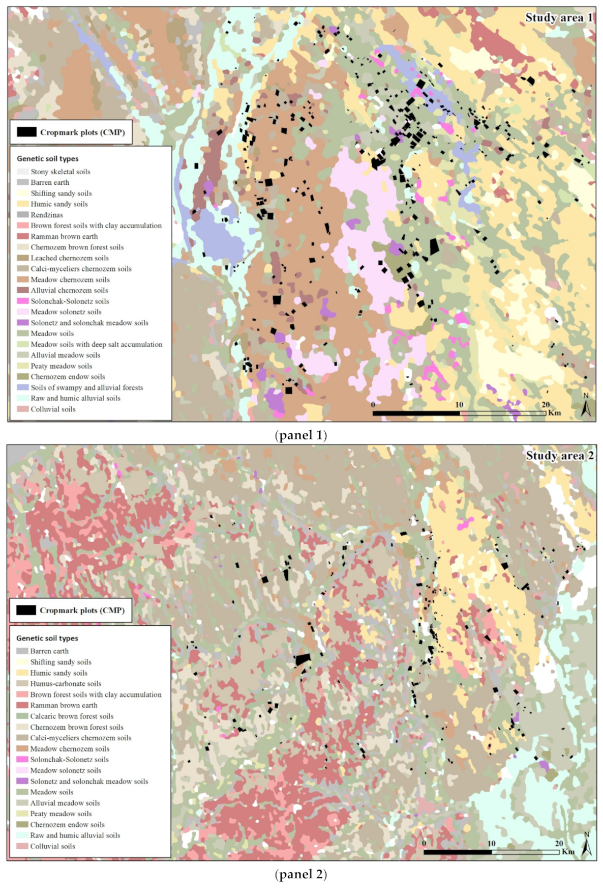
The eastern part of study area 1 (Figure 4, first panel) is dominated by an alluvial fan covered with sandy soils, and the amount of the detected CMPs decreases. Furthermore, in the case of the area derived from the fan, the CMPs were not recognizable on salt-affected soils. Only rarely do a few cropmarks show up on alluvial soils close to the riverbanks.
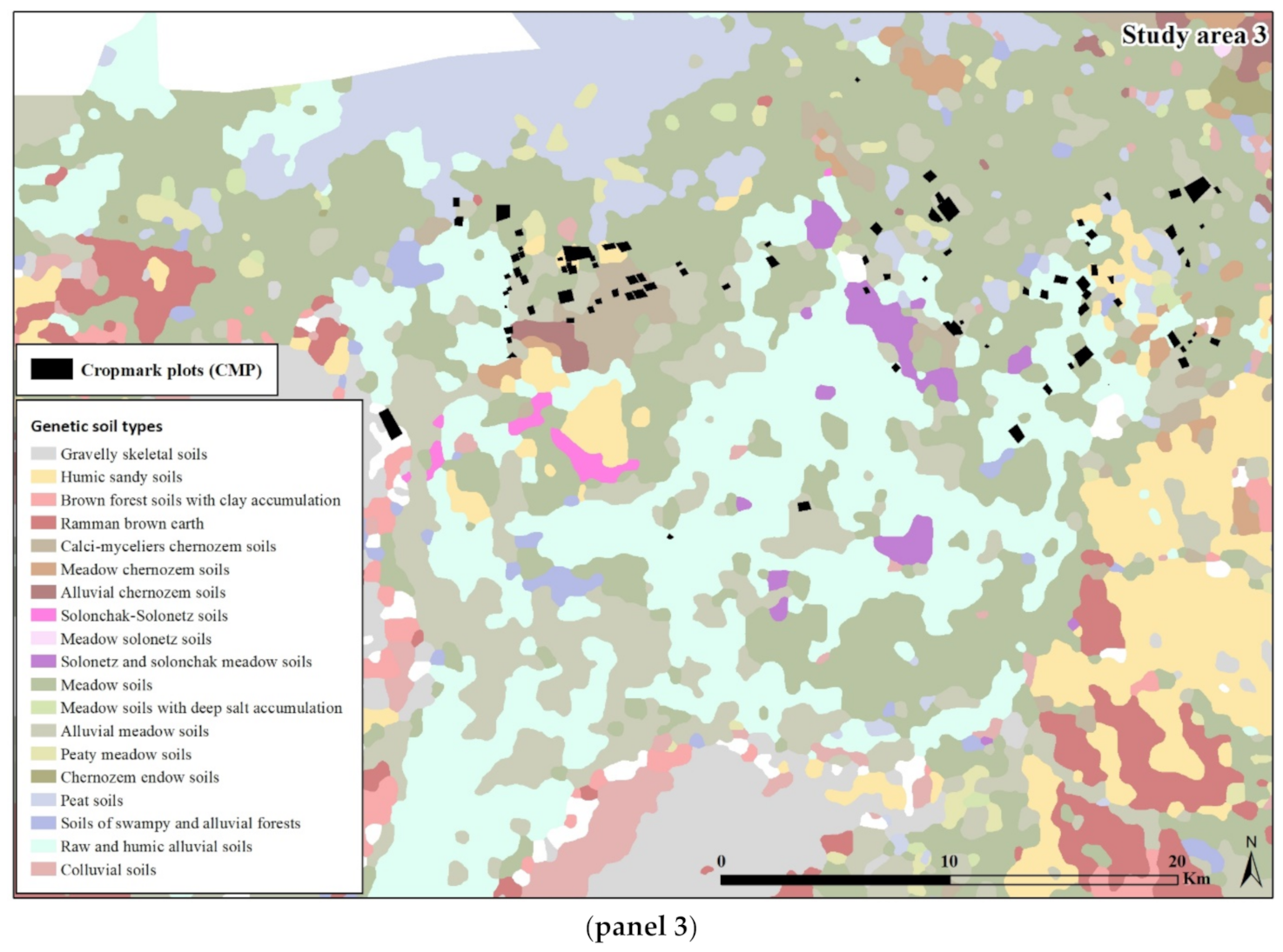
Study area 2 (Figure 4, second panel) is the most geomorphologically determined area of the three study areas. The cropmarks fit in the typical soil types of valley floors, and in the vast majority of cases, the CMPs occur on Chernozem soils. As with previous study areas, only a few CMPs could be detected on sandy soils. Study area 3 (Figure 4, third panel) is the most heterogeneous area in relation to the distribution of soil types. The majority of CMPs occur on Meadow and Chernozem type soils. It is suggested that the detection of CMPs depends mainly on the weather and seasons.
3.2. Differences between Pedological Characteristics of CMPs and nCMPs as Revealed by the Kolmogorov–Smirnov Test
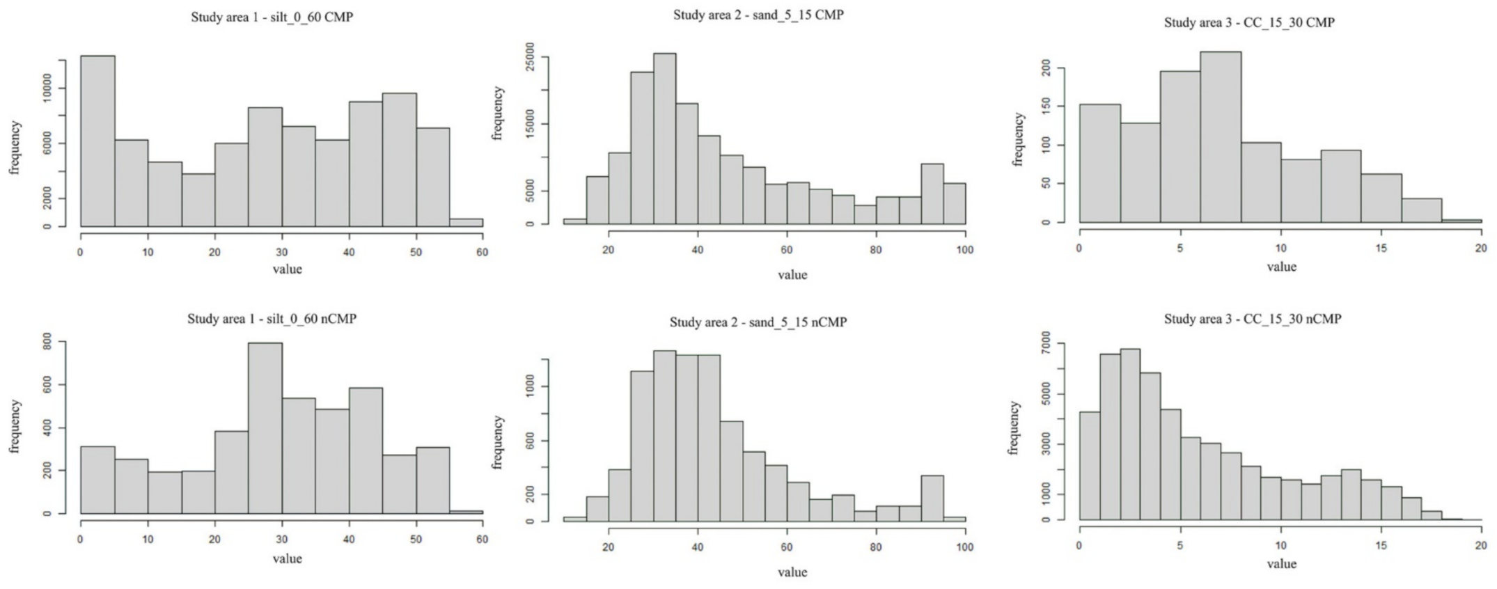
In the light of the two-sample Kolmogorov–Smirnov homogeneity tests, the three pilot areas display significant differences. The ranked soil properties are listed in Table S1. For each study area, the histogram of the raster cell values for the two data sets (CMPs and nCMPS) in the case of the most discriminating soil properties are displayed in Figure 5.
In the Rába interfluve study area, CMPs and nCMPs mostly differ in the carbonate content of the upper layers. Particle size fractions (clay, sand and silt content) in subsoil (under 1m) and near-surface soil organic carbon also seem to be strong discriminating factors. As can be seen in Figure 5, the carbonate content of the 15–30 cm layer is shifted towards higher values in CMPs, with the distribution reaching a maximum in the 6-8% range; however, a second, local maximum is similarly situated for both data sets at about 13%.
In the Sió-Sárvíz study area CMPs and nCMPs differ mostly in the particle size fractions (clay, sand and silt content) of all layers; carbonate and soil organic matter content lag behind and seem to be rather weak discriminating factors. Despite the significant test result, the histograms in Figure 5 do not seem to differ to any great extent, except for the fact that for CMPs the maximum close range sand content of the 5–15 cm layer is wider, and at over 40% is still almost as high as at 30%.
In the Danube-Tisza interfluve study area, CMPs and nCMPs also differ to a large extent in particle size fractions (clay, sand and silt content). However, deeper layers occur later in the ranking; carbonate and soil organic matter content even lag behind and seem to be rather loose discriminating factors. The two histograms in Figure 5 for the silt content of the 0–60 cm layer look rather different, while for CMPs the maximum is located at the lowest values and the overall distribution shows only slight fluctuations. For nCMPs the maximum is close to 30% and only one mode is visible.
It is an interesting fact that for all the three study areas rooting depth showed very weak discriminating power, while pH and bulk density did not provide any statistically valid test results despite their presupposed higher significance.
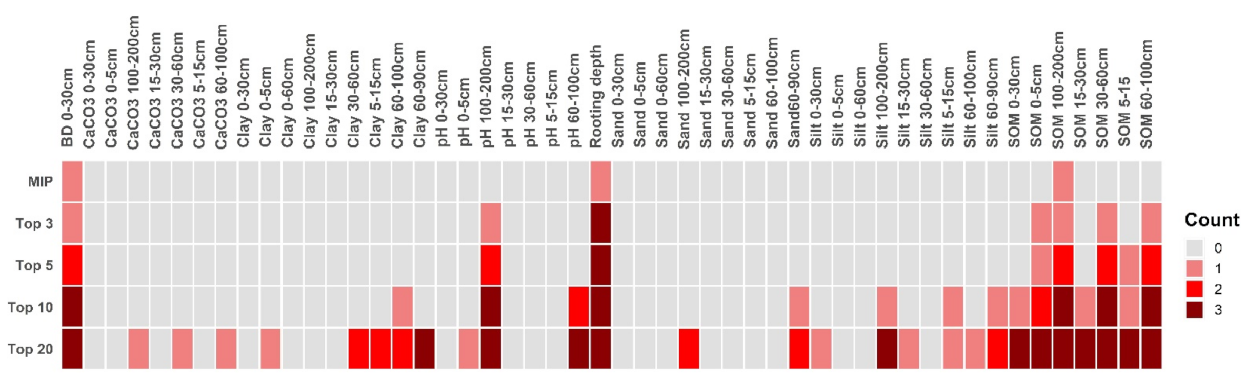
For all three study areas, the use of RF with genetic soil type as qualitative predictor provided the same results in relation to the importance of soil type, ranking it in the hindmost position. As a consequence, the result and discussion of the models excluding soil type alone form the focus of the discussion. Variable ranks are listed in Table S2. They are also displayed graphically for each study area in Figure S1 [48].
In the Rába interfluve study area the most important soil properties in the prediction of CMPs and nCMPs are the soil organic matter content of the deeper layers, rooting depth, pH of the subsoil (under 1 m) and bulk density of the topsoil (0–30 cm).
In the Sió-Sárvíz valley study area, the most important soil properties in the prediction of CMPs and nCMPs are rooting depth, soil organic matter content of the deeper layers, pH of the subsoil (under 1 m), bulk density of the topsoil (0–30 cm).
In the Danube-Tisza interfluve study area the most important soil properties in the prediction of CMPs and nCMPs are bulk density of the topsoil (0–30 cm), soil organic matter content of the topmost layers (0–5 and 5–15 cm), rooting depth, pH of the subsoil (under 1m), the soil organic matter content of the deeper layers.
It is an interesting point that particle size fractions (clay, sand and silt content) lag behind in all three study areas, while in KS they were top ranked, and the least discriminating properties provide by KS became the determining factors in the RF based prediction of CMPs (Figure 6).
4. Discussion
Although in the selection of the study areas, the aim was to match as many criteria as possible, it should be noted that it is not yet possible to guarantee the same level of analysis of the areas, and they thus cannot be compared with a perfect level of consistency in terms of cropmark formation conditions. This is primarily due to the weather factor, which shows considerable variations every year for the three study areas. While in the area of the Danube-Tisza interfluve cropmarks can be detected every year, there are years when their discovery is not possible in the Rába interfluve. The Sió/Sárvíz valley falls somewhere in between these two, as there are no completely unsuccessful years, but truly good ones are rare as well. A further weather-related observation is that the periods ideal for identifying cropmarks—the cropmark time-windows—are not of the same length in the case of each study area. In the Danube-Tisza interfluve study area, there may be a relatively long period of up to two months, whereas this period is noticeably shorter in the Sió / Sárvíz valley, and only 1–2 weeks long in the Rába interfluve. A further complicating factor in the case of the Sió / Sárvíz valley is that the maize/sunflower/rape trio plays a noticeably greater role in field crop production than in the other areas. This means that barley/wheat are grown less frequently in crop rotation than in the other two study areas. Finally, it should be noted that the research of the Danube-Tisza interfluve is much cheaper due to its proximity to the bases of the researchers. Thus, even in the years of scarce funding, flights were guaranteed, while good years—like 2012—may have been missed in the other two areas (Table 2).
Also due to these differences, the proportion of areas covered by CMP is significantly higher in the Danube-Tisza interfluve than in the other two study areas. It is possible that further flights will reduce the differences in representativeness between the study areas, eventually making the results of the statistical analyses more coherent regardless of the study areas.
Although all three sample areas have alluvial fan origins, their sediment accumulation and surface evolution show distinct features. Their geologic and geomorphologic diversity makes it difficult to specify factors that influence the cropmark appearance clearly. Because of the different appearance of geomorphological/sedimentological fragmentation, determining soil-parameters can still be used to boost the effectiveness of identifying cropmarks.
Regarding the occurrence of CMP-nCMP, the topsoil bulk density and the grain-size composition can be definitive on areas of fluvially determined low angle fans with a complex recent geomorphologic history. On these surfaces diverse landforms are built up from sediments differing greatly in their water-balance, resulting in a mosaic of sand regions, wet meadows, terrace surfaces and floodplains (e.g., the Danube-Tisza interfluve). As sand movement and fluvial land-forming have been active processes during the Holocene, [49] both the subsurface sediments and the topsoil display great spatial variability.
The situation/picture/ is different in areas where during the Late Quaternary surface evolution was governed by shallow valleys cutting into alluvial fans (e.g., the Sió-Sárvíz valley): in the dual fluviatile system of floodplains and flood-free relief areas, the topsoil bulk density is also an important factor. But the dominant component yielding sediment and forming surfaces is sediment accumulation related to the recent flooding of active streams. This therefore results in significantly higher organic material and carbonate content as CMP-nCMP markers.
Regarding the CMP-nCMP analyses, the most problematic areas are completely flat plains with origins as alluvial fan. Considering sedimentation and buried paleo-landforms together, the area must be considered fragmented. These terrains covered in thick, alluvial sediments partially Holocene in origin are characterized by invariable reliefs [50]. The majority of paleochannels are completely buried by now (e.g., in the Rába interfluve). As today’s surface does not reflect the earlier, rougher terrain, and because of its covering alluvial sediment, higher organic material and carbonate content seem to be even more dominant factors in defining CMP and nCMP areas.
Pedological differences between CMPs and nCMPs can be detected by all the three approaches. The statistically identified differences, however, differ to a fair degree between the various approaches. Differences in the distribution of specific soil property values for CMPs and nCMPs (as opposed to the variable importance provided by RF for the prediction of the two types of areas) result in significantly different rankings of soil properties. This might be caused by the problem of representative sampling in the study areas.
In contrast to results for the Czech Republic [16,19], those presented here do not show the dominance of sandy soils in cropmarks.
The role of soil chemical properties in cropmarks revealed by Hejcman et al. (2013) [27] are, however, supported by the result in the present study that organic matter and carbonate as well as pH are important variables in RF models. However, nutrients available to plants have not been mapped in the frame of DOSoReMI.hu due to their dynamic nature and the lack of available observational data. Thus, their role in cropmarks is not considered in the present work. Nevertheless, the approach employed can reveal the more static pedological background where the spatial differences in nutrient status due to archeological sources may result in stronger effects on crop development, thus making plots more suitable for cropmarks.
5. Conclusions
The analyses of the factors behind the formation of cropmarks gave rather complex results, despite the fact that only the fixed elements of the system were examined. The importance of alluvial fans has also been prospected in Southern Germany, Switzerland, Austria, and the Czech Republic. However, the differences in cropmark between alluvial fan sub-types have been explained by analyzing Hungarian soil data. At the same time, this method could prove useful in the future for the analysis of areas with significantly different geomorphological conditions—bearing in mind the important role of loess areas in the Czech Republic.
Based on the detailed statistical analysis of both the aerial archaeological and pedological data, different factors seem to be relevant to each study area. However, these differences can be sufficiently explained by the slightly different formation and landscape evolution processes of study areas with similar bedrock. While cropmarks correlate well with the results of traditional soil mapping, much more complex processes underlie the formation of cropmarks. This is probably due to the fact that in previous analyses, the role of some important factors (e.g., sandy soils) seems to have been more subordinate.
Since the 1990s, Hungary has been considered highly suitable for the prospection of cropmarks, thanks chiefly to the presence of large field monoculture grain corn production and also to early summer weather suitable for aerial archaeological research. Among a number of other factors, the favorable conditions can certainly be linked to a high-quality soil mantle. It is worth noting that by increasing the representativeness of archaeological prospecting, an even more accurate picture may hopefully be created in the future. One important objective of the methodological developments presented here is the creation of a predictive model in order to start mapping cropmarks during flights over micro-regions not previously researched, but in which the geomorphological / soil conditions seem to be favorable.
We also plan to explore the roles of changeable factors. The above described features’ influence on cropmarks might be enhanced, decreased, or—in years of extreme weather— completely altered by weather conditions, especially by the amount of precipitation.
The use of cropmarks in aerial archaeology helps primarily the identification and the geomorphological analyses of sites, as well as the mapping of archaeological data. However, in order to understand the complex factors of cropmark formation better, new methods were needed. Asked in 2000 how much experience he needed truly to understand the nature and the research opportunities of cropmarks, René Goguey's answer was: “After 30 years work, I’ve started to realize”. Now, 20 years later, progress seems possible on the basis of an approach which makes cropmark data suitable for statistical processing, together with analyses related to soil data systems based on remote sensing data sources and interpreted from a geomorphological point of view. It is the hope of the authors that the methodological experiments detailed here may make the technology of aerial archaeological prospecting, which has been somewhat sidelined in the last 10 years, more predictable, plannable and thereby more effective.
Supplementary Materials
The following are available online at https://www.mdpi.com/2072-4292/13/6/1126/s1, Table S1: Rank of primary soil property maps used for the comparison of the pedological features of CMPs and nCMPs in the case of the three study areas. The higher the D value, the greater the degree to which CMPs and nCMPs differed in their tested soil properties. Table S2: Variable importance rank of primary soil properties used in Random Forest modelling of CMPs and nCMPs in the case of the three study areas. The higher the importance value, the more informative is the given soil property in the discrimination of CMPs and nCMPs. Figure S1: Variable importance rank of primary soil properties used in Random Forest modelling of CMPs and nCMPs in the case of the three test sites.
Author Contributions
Conceptualization, Z.C. and L.P.; methodology, Z.C., B.N. and L.P.; software, M.Á. and J.M.; validation, Z.C., B.N. and L.P.; formal analysis, Z.C.; investigation, Z.C. and L.P.; resources, Z.C. and L.P.; data curation, M.Á., J.M. and L.R.; writing—original draft preparation, Z.C. B.N. and L.P.; writing—review and editing, Z.C., B.N. and L.P.; visualization, M.Á., J.M. and L.R.; supervision, Z.C. and L.P.; project administration, Z.C.; funding acquisition, Z.C. and L.P. All authors have read and agreed to the published version of the manuscript.
Funding
This research was funded by National Research Development and Innovation Office (Hungary), grant numbers NN-111058, K-131820 and SNN 134635, by the Higher Educational Institutional Excellence Program / the Thematic Excellence Program of the Eötvös Loránd University, and Momentum Mobility research project (Institute of Archaeology, Research Centre for the Humanities), granted by the Momentum Program of the Hungarian Academy of Sciences.
Data Availability Statement
The digital soil maps used in the present study were compiled in the “Digital Optimized Soil Related Maps and Information” framework and are published on the www.dosoremi.hu website. The maps were elaborated according to GSM specifications, thus they also represent the Hungarian contribution to the GlobalSoilMap.net project. The CMPs are sensitive data containing archaeological site information indirectly.
Acknowledgments
The authors thank Á. Marton for his indispensable contribution. We are grateful to the editors and the six anonymous reviewers who provided valuable suggestions regarding the manuscript.
Conflicts of Interest
The authors declare no conflict of interest.
References
- Goguey, R. Traces dans la Grande Plaine...Photographies Aériennes de Hongrie. Exposition du 18 Avril au 2 Juin 2002; Conseil Général du Rhône: Saint-Romain-en-Gal-Vienne, France, 2002. [Google Scholar]
- Barber, M. A History of Aerial Photography and Archaeology. Mata Hari’s Glass Eye and Other Stories; English Heritage: Swindon, UK, 2011; ISBN 978-1-848020-36-8. [Google Scholar]
- Crawford, O.G.S. Air Survey and Archæology. Geogr. J. 1923, 61, 342–360. [Google Scholar] [CrossRef]
- Neogrády, S. A légifénykép és az archeológiai kutatások [The aerial photo and the archaeological survey]. Térképészeti Közlöny 1950, 7, 283–332. [Google Scholar]
- Christlein, R.; Braasch, O. Das Unterirdische Bayern. 7000 Jahre Geschichte und Archäologie im Luftbild; Theiss: Stuttgart, Germany, 1990; ISBN 3-8062-0855-7. [Google Scholar]
- Cowley, D.C. Creating the Cropmark Archaeological Record in East Lothian, South-East Scotland. In Prehistory without Borders. The Prehistoric Archaeology of the Tyne–Forth Region; Crellin, R., Fowler, C., Tipping, R., Eds.; Oxbow Books: Oxford, UK, 2016; pp. 59–70. ISBN 978-1-78570-200-6. [Google Scholar]
- Dabas, M.; Delétang, H.; Ferdière, A.; Jung, C.; Zimmermann, W.H. La Prospection; Errance: Paris, France, 1998; ISBN 2-87772-160-4. [Google Scholar]
- Braasch, O. Vom heiteren Himmel…Luftbildarchäologie; Gesellschaft für Vor-und Frühgeschichte Württemberg und Hohenzollern e.V.: Esslingen, Germany, 2005; ISBN 3-9808926-1-1. [Google Scholar]
- Scollar, I. Archaeological Prospecting and Remote Sensing; Cambridge University Press: Cambridge, UK, 1990; ISBN 10: 052132050X. [Google Scholar]
- Verhoeven, G.J. Near-Infrared Aerial Crop Mark Archaeology: From its Historical Use to Current Digital Implementations. J. Archaeol. Method Theory 2012, 19, 132–160. [Google Scholar] [CrossRef]
- Luo, L.; Wang, X.; Guo, H.; Lasaponara, R.; Zong, X.; Masini, N.; Wang, G.; Shi, P.; Khatteli, H.; Chen, F.; et al. Airborne and spaceborne remote sensing for archaeological and cultural heritage applications: A review of the century (1907–2017). Remote Sens. Environ. 2019, 232, 111280. [Google Scholar] [CrossRef]
- Verhoeven, G.; Sevara, C. Trying to break new ground in aerial archaeology. Remote Sens. 2016, 8, 918. [Google Scholar] [CrossRef] [Green Version]
- Verhoeven, G.J. Are we there yet? A review and assessment of archaeological passive airborne optical imaging approaches in the light of landscape archaeology. Geosciences 2017, 7, 86. [Google Scholar] [CrossRef] [Green Version]
- Cowley, D.C. Aerial photographs and aerial reconnaissance for landscape studies. In Detecting and Understanding Historical Landscapes; Chavarría Arnau, A., Reynolds, A., Eds.; SAP Societā Archeologica: Mantova, Italy, 2015; pp. 37–66. ISBN 978-88-87115-99-4. [Google Scholar]
- Cowley, D.C.; Stichelbaut, B.B. Historic Aerial Photographic Archives for European Archaeology. Eur. J. Archaeol. 2012, 15, 217–236. [Google Scholar] [CrossRef]
- Hejcman, M.; Smrž, Z. Cropmarks in stands of cereals, legumes and winter rape indicate sub-soil archaeological features in the agricultural landscape of Central Europe. Agric. Ecosyst. Environ. 2010, 138, 348–354. [Google Scholar] [CrossRef]
- Czajlik, Z. Les possibilités de la prospection aérienne conventionnelle en Hongrie. In Studia Celtica Classica et Romana Nicolae Szabó Septuagesimo Dedicata; Pytheas: Budapest, Hungary, 2012; pp. 80–96. ISBN 978-963-9746-77-0. [Google Scholar]
- Leidorf, K. Luftbildarchäologie—Geschichte und Methode. In Archäologische Prospektion. Luftbildarchäologie und Geophysik. Arbeitshefte des Bayerischen Landesamtes für die Denkmalpflege, Band 59; Becker, H., Ed.; Bayerisches Landesamt für Denkmalpflege: München, Germany, 1996; pp. 33–44. ISBN 3-87490-541-1. [Google Scholar]
- Gojda, M.; Hejcman, M. Cropmarks in main field crops enable the identification of a wide spectrum of buried features on archaeological sites in Central Europe. J. Archaeol. Sci. 2012, 39, 1655–1664. [Google Scholar] [CrossRef]
- Stanjek, H.; Faßbinder, J.W.E. Soil aspects affecting archaeological details in aerial photographs. Archaeol. Prospect. 1995, 2, 91–101. [Google Scholar] [CrossRef]
- Evans, R.; Jones, R.J.A. Crop marks and soils at two archaeological sites in Britain. J. Archaeol. Sci. 1977, 4, 63–76. [Google Scholar] [CrossRef]
- Braasch, O.; Kaufmann, D. Zum Beginn archäologischer Flugprospektion in Sachsen-Anhalt. Ausgrab. Funde 1992, 4, 186–205. [Google Scholar]
- Czajlik, Z.; Bödőcs, A. The Effectiveness of Aerial Archaeological Research—An Approach from the GIS Perspective. In Moments in Time. Papers Presented to Pál Raczky on His 60th Birthday; l’Harmattan: Budapest, Hungary, 2013; pp. 873–883. ISBN 978-963-236-346-2. [Google Scholar]
- Linck, R.; Abandowitz, S.; Leidorf, K. Mitten im Mais: Rekordsommer enthüllt Grabenwerke mittels Luftbildarchäologie. Das archäologische Jahr Bayern 2018, 38, 163–166. [Google Scholar]
- Leckebusch, J.; Nagy, P. Propektionsmethoden in der Archäologie; Stiftung für die Erforschung des Üetlibergs: Zürich, Switzerland, 1991. [Google Scholar]
- Doneus, M. Luftbildarchäologie und Photogrammetrie am Institut für Ur-und Frühgeschichte in Wien. In Luftbildarchäologie in Ost-und Mitteleuropa. Aerial Archaeology in Eastern and Central Europe. Internationales Symposium 26.–30. September 1994 Kleinmachnow. Land Brandenburg, Forschungen zur Archäologie im Land Brandenburg 3; Verlag Brandenburgisches Landesmuseum für Ur-und Frühgeschichte: Potsdam, Germany, 1995; pp. 123–132. [Google Scholar]
- Hejcman, M.; Součková, K.; Gojda, M. Prehistoric settlement activities changed soil pH, nutrient availability, and growth of contemporary crops in Central Europe. Plant Soil 2013, 369, 131–140. [Google Scholar] [CrossRef]
- Evans, R. The weather and other factors controlling the absence of crop marks on clay and „difficult” soils. In Populating Clay Landscapes; Tempus: Stroud, UK, 2007; pp. 16–27. [Google Scholar]
- Doneus, M. Die hinterlassene Landschaft—Prospektion und Interpretation in der Landschaftsarchäologie. Mitteilungen der Prähistorischen Kommission Band 78; Österreichisch Akademie der Wissenschaften: Wien, Austria, 2013; ISBN 978-3-7001-7197-3. [Google Scholar]
- Gábris, G.; Nádor, A. Long-term fluvial archives in Hungary: Response of the Danube and Tisza rivers to tectonic movements and climatic changes during the Quaternary: A review and new synthesis. Quat. Sci. Rev. 2007. [Google Scholar] [CrossRef]
- Gábris, G.; Nagy, B. Climate and tectonically controlled river style changes on the Sajó-Hernád alluvial fan (Hungary). In Alluvial Fans: Geomorphology, Sedimentology, Dynamics—Introduction. A Review of Alluvial-Fan Research; Geological Society: London, UK, 2005; pp. 61–67. [Google Scholar]
- Vogel, H.J.; Bartke, S.; Daedlow, K.; Helming, K.; Kögel-Knabner, I.; Lang, B.; Rabot, E.; Russell, D.; Stößel, B.; Weller, U.; et al. A systemic approach for modeling soil functions. Soil 2018, 4, 83–92. [Google Scholar] [CrossRef] [Green Version]
- Miller, B.A.; Schaetzl, R.J. The historical role of base maps in soil geography. Geoderma 2014, 230–231, 329–339. [Google Scholar] [CrossRef]
- Heuvelink, G.B.M.; Webster, R. Modelling soil variation: Past, present, and future. Geoderma 2001, 100, 269–301. [Google Scholar] [CrossRef]
- Várallyay, G. Soil mapping in Hungary. Agrokémia Talajt 1989, 38, 696–714. [Google Scholar]
- Minasny, B.; McBratney, A.B. Digital soil mapping: A brief history and some lessons. Geoderma 2016. [Google Scholar] [CrossRef]
- McBratney, A.B.; Mendonça Santos, M.L.; Minasny, B. On Digital Soil Mapping. Geoderma 2003, 117, 3–52. [Google Scholar] [CrossRef]
- Pásztor, L.; Laborczi, A.; Takács, K.; Illés, G.; Szabó, J.; Szatmári, G. Progress in the elaboration of GSM conform DSM products and their functional utilization in Hungary. Geoderma Reg. 2020, 21, e00269. [Google Scholar] [CrossRef]
- Whimster, R. The Emerging Past. Air Photography and the Buried Landscape; Royal Comission on the Historical Monuments of England: Abingdon, UK, 1989; ISBN 095072369. [Google Scholar]
- Cowley, D.; Gilmour, S.M.D. Some observations on the nature of aerial survey. In From the Air: Understanding Aerial Archaeology; Tempus Publishing: Stroud, UK, 2005; pp. 50–63. ISBN 0-7524-3130-7. [Google Scholar]
- Hanson, W.S. Sun, sand and see: Creating bias in the archaeological record. In From the Air: Understanding Aerial Archaeology; Tempus Publishing: Stroud, UK, 2005; pp. 73–85. ISBN 0-7524-3130-7. [Google Scholar]
- Szabó, M. Archaeology from Above; Archaeolingua: Budapest, Hungary, 2016; ISBN 978-963-9911-86-4. [Google Scholar]
- Tanács, E.; Belényesi, M.; Lehoczki, R.; Pataki, R.; Petrik, O.; Standovár, T.; Pásztor, L.; Laborczi, A.; Szatmári, G.; Molnár, Z.; et al. Országos, nagyfelbontású ökoszisztéma-alaptérkép: Módszertan, validáció és felhasználási lehetőségek. Természetvédelmi Közlemények 2019, 25, 34–58. [Google Scholar] [CrossRef]
- Brevik, E.C.; Calzolari, C.; Miller, B.A.; Pereira, P.; Kabala, C.; Baumgarten, A.; Jordán, A. Soil mapping, classification, and pedologic modeling: History and future directions. Geoderma 2016. [Google Scholar] [CrossRef]
- Pásztor, L.; Laborczi, A.; Bakacsi, Z.; Szabó, J.; Illés, G. Compilation of a national soil-type map for Hungary by sequential classification methods. Geoderma 2018. [Google Scholar] [CrossRef] [Green Version]
- Breiman, L. Random forests. Mach. Learn. 2001. [Google Scholar] [CrossRef] [Green Version]
- Hengl, T.; De Jesus, J.M.; Heuvelink, G.B.M.; Gonzalez, M.R.; Kilibarda, M.; Blagotić, A.; Shangguan, W.; Wright, M.N.; Geng, X.; Bauer-Marschallinger, B.; et al. SoilGrids250m: Global gridded soil information based on machine learning. PLoS ONE 2017, 12, e0169748. [Google Scholar] [CrossRef] [PubMed] [Green Version]
- Szatmári, G.; Bakacsi, Z.; Laborczi, A.; Petrik, O.; Pataki, R.; Tóth, T.; Pásztor, L. Elaborating Hungarian Segment of the Global Map of Salt-Affected Soils (GSSmap): National Contribution to an International Initiative. Remote Sens. 2020, 12, 4073. [Google Scholar] [CrossRef]
- Gábrís, G.; Horváth, E.; Novothny, Á.; Ruszkiczay-Rüdiger, Z. Fluvial and aeolian landscape evolution in Hungary—Results of the last 20 years research. Geol. en Mijnbouw/Neth. J. Geosci. 2012. [Google Scholar] [CrossRef] [Green Version]
- Czajlik, Z.; Rupnik, L.; Losonczi, M.; Timár, L. Aerial archaeological survey of a buried landscape: The Tóköz project. In Remote Sensing for Archaeological Heritage Management, Proceedings of the 11th EAC Heritage Management Symposium, Reykjavik, Iceland, 25–27 March 2010; Archaeolingua: Brussels, Belgium, 2011; pp. 235–241. ISBN 978-963-9911-20-8. [Google Scholar]
Figure 1.
Dabas—Öreg Országúti-dűlő (Pest County, Hungary) aerial archaeological site. The image is dominated by the positive cropmarks showing the color variations (marks of a green circular ditch and small pits) in yellow wheat. On the right side, mostly due to the barley’s late harvest period, some further pits are visible (cf. Figure 2) owing to shadow effect of the cropmarks (Oblique aerial photograph, 12 June 2015, Zoltán Czajlik).

Figure 2.
Rectified oblique aerial photographs at Dabas—Öreg Országúti-dűlő (Pest County, Hungary, cf. Figure 1). Aerial photo polygons are generally related to the parcel-system. The “normal”/late harvest cropmarks are marked in different colors. Source: Zoltán Czajlik, 12 June 2015 and GE-imagery.

Figure 3.
Location of the study areas. Cropmark plots (CMPs) are displayed in yellow.

Figure 4.
(panel 1–3). Distribution of CMPs on the soil type map for the study areas.


Figure 5.
The histograms of the raster cell values for the two data sets (CMPs and nCMPS) in the case of the most discriminating soil properties for the three study areas.
Figure 5.
The histograms of the raster cell values for the two data sets (CMPs and nCMPS) in the case of the most discriminating soil properties for the three study areas.

Figure 6.
Importance of soil property covariates for predicting the indicators of CMPs and nCMPs. Abbreviations: BD: bulk density, SOM: soil organic matter content.
Figure 6.
Importance of soil property covariates for predicting the indicators of CMPs and nCMPs. Abbreviations: BD: bulk density, SOM: soil organic matter content.


Table 1.
Summary of the primary soil property maps used for the comparison of the pedological features of CMPs and nCMPs.
Table 1.
Summary of the primary soil property maps used for the comparison of the pedological features of CMPs and nCMPs.
| Soil Properties Linked to Layers | GSM.net Depth Intervals [cm] | Equidistant Depths [cm] | Topsoil | |||||||
|---|---|---|---|---|---|---|---|---|---|---|
| 0–5 | 5–15 | 15–30 | 30–60 | 60–100 | 100–200 | 0–30 | 30–60 | 30–60 | 0–60 | |
| soil organic matter [%] (SOM) | x | x | x | x | x | x | x | x | ||
| pH | x | x | x | x | x | x | x | x | ||
| bulk density [g/cm3] (BD) | x | |||||||||
| sand [%] | x | x | x | x | x | x | x | x | x | x |
| silt [%] | x | x | x | x | x | x | x | x | x | x |
| clay [%] | x | x | x | x | x | x | x | x | x | x |
| CaCO3 [%] (CC) | x | x | x | x | x | x | x | x | ||
| Soil properties linked to soil profile | ||||||||||
| genetic soil type (traditional) | x | |||||||||
| rooting depth [cm] | x | |||||||||
Table 2.
Comparison of the cropmark investigation circumstances and the proportions of CMP/nCMP of the study areas.
Table 2.
Comparison of the cropmark investigation circumstances and the proportions of CMP/nCMP of the study areas.
| Danube–Tisza Interfluve | Sió–Sárvíz Valley | Rába Interfluve | |
|---|---|---|---|
| area (km2) | 2144 | 2824 | 809 |
| general time window | 8–10 weeks | 5–6 weeks | 1–2 weeks |
| seasonal differences | not significant | medium | significant |
| total CMP [ha] | 4339 | 2440 | 1070 |
| total nCMP [ha] | 81303 | 170885 | 51469 |
| proportion CMP [ha] | 5.34 | 1.43 | 2.08 |
| proportion nCMP [ha] | 94.66 | 98.57 | 97.92 |
Publisher’s Note: MDPI stays neutral with regard to jurisdictional claims in published maps and institutional affiliations. |
© 2021 by the authors. Licensee MDPI, Basel, Switzerland. This article is an open access article distributed under the terms and conditions of the Creative Commons Attribution (CC BY) license (http://creativecommons.org/licenses/by/4.0/).
Share and Cite
MDPI and ACS Style
Czajlik, Z.; Árvai, M.; Mészáros, J.; Nagy, B.; Rupnik, L.; Pásztor, L. Cropmarks in Aerial Archaeology: New Lessons from an Old Story. Remote Sens. 2021, 13, 1126. https://doi.org/10.3390/rs13061126
AMA Style
Czajlik Z, Árvai M, Mészáros J, Nagy B, Rupnik L, Pásztor L. Cropmarks in Aerial Archaeology: New Lessons from an Old Story. Remote Sensing. 2021; 13(6):1126. https://doi.org/10.3390/rs13061126
Chicago/Turabian StyleCzajlik, Zoltán, Mátyás Árvai, János Mészáros, Balázs Nagy, László Rupnik, and László Pásztor. 2021. "Cropmarks in Aerial Archaeology: New Lessons from an Old Story" Remote Sensing 13, no. 6: 1126. https://doi.org/10.3390/rs13061126
Note that from the first issue of 2016, this journal uses article numbers instead of page numbers. See further details here.