
Boundary-Assisted Learning for Building Extraction from Optical Remote Sensing Imagery


1
State Key Laboratory of Information Engineering in Surveying, Mapping and Remote Sensing, Wuhan University, Wuhan 430079, China
2
Collaborative Innovation Center of Geospatial Technology, Wuhan University, Wuhan 430079, China
*
Author to whom correspondence should be addressed.
Remote Sens. 2021, 13(4), 760; https://doi.org/10.3390/rs13040760
Submission received: 10 January 2021
/
Revised: 10 February 2021
/
Accepted: 15 February 2021
/
Published: 18 February 2021
(This article belongs to the Special Issue Advanced Artificial Intelligence and Deep Learning for Remote Sensing)
Abstract
:Deep learning methods have been shown to significantly improve the performance of building extraction from optical remote sensing imagery. However, keeping the morphological characteristics, especially the boundaries, is still a challenge that requires further study. In this paper, we propose a novel fully convolutional network (FCN) for accurately extracting buildings, in which a boundary learning task is embedded to help maintain the boundaries of buildings. Specifically, in the training phase, our framework simultaneously learns the extraction of buildings and boundary detection and only outputs extraction results while testing. In addition, we introduce spatial variation fusion (SVF) to establish an association between the two tasks, thus coupling them and making them share the latent semantics and interact with each other. On the other hand, we utilize separable convolution with a larger kernel to enlarge the receptive fields while reducing the number of model parameters and adopt the convolutional block attention module (CBAM) to boost the network. The proposed framework was extensively evaluated on the WHU Building Dataset and the Inria Aerial Image Labeling Dataset. The experiments demonstrate that our method achieves state-of-the-art performance on building extraction. With the assistance of boundary learning, the boundary maintenance of buildings is ameliorated.
1. Introduction
Building extraction from optical remote sensing imagery is one of the fundamental tasks in remote sensing, which plays a key role in many applications, such as urban planning and construction, natural crisis and disaster management, and population and regional development [1,2,3]. The years of development of Earth observation technology have made high-quality remote sensing images available, and the spatial resolution and elaborate spectral, structure, and texture information of objects are increasingly being represented [4]. These make various objects in the imagery distinguishable and make accurate extraction of buildings possible. Meanwhile, the amount of remote sensing imagery is increasing rapidly, which puts forward a high demand for automatic image processing.
During the past several decades, the major methods for building extraction from aerial or satellite imagery consisted of designing features (spectrum, edge, shape, shadow, and so on) that could best represent buildings [5]. For example, Huang et al. [6] utilized the intrinsic spectral–structural properties of buildings and proposed the morphological building index. Wang et al. [7] introduced a semi-automatic building extraction method by tracking the edge and linear features. Hu et al. [8] proposed an enhanced morphological building index for automatic building extraction based on shape characteristics. Ok et al. [9] modeled the directional spatial relationship between buildings and their shadows. Those methods have made some achievements, but only work under certain conditions, as the features are handcrafted, and such empirically designed features have poor generalization ability.
In recent years, deep learning techniques [10], especially convolutional neural networks (CNNs), have been applied to many fields and have shown important implications in the field of computer vision. CNNs automatically and efficiently learn hierarchical features that map the original inputs to the designated labels without any prior knowledge. Due to their powerful feature representation ability, CNNs outperform traditional approaches by leaps and bounds in many vision missions [11]. Early CNNs [12,13,14] focused on the classification of whole images, but lacked accurate identification and positioning of objects in images. Since Long et al. [15] first put forward fully convolutional networks (FCNs), semantic segmentation, a pixel-level classification task [16] that aims to assign each pixel to the class of its enclosing object, has been dramatically developed. Based on the FCN paradigm, a large variety of state-of-the-art (SOTA) FCN frameworks have been proposed to improve the segmentation performance. For example, the encoder–decoder network (SegNet [17]) adopts elegant structures to better recover object details. Multi-scale networks (PSPNet [18], DeepLab [19]) extract information from feature maps of various scales to fit in with objects of different sizes. Networks with skip connections (SharpMask [20], U-Net [21]) combine multi-level features to generate crisp segmentation maps. These classic FCNs have made significant achievements on natural scene or medical image datasets, such as PASCAL VOC [22], Microsoft COCO [23], and BACH [24].
Inspired by the great success of CNNs in computer vision, researchers have extended them to remote sensing image processing [25]. Building extraction, which can be settled via semantic segmentation, has also benefited a lot from FCNs. For example, Yi et al. [26] modified the U-Net [21], proposing an encoder–decoder network to perform urban building segmentation. Maggiori et al. [27] developed a multi-scale structure in an FCN to reduce the tradeoff between recognition and precise localization. Ji et al. [5] proposed a Siamese structure that takes an original image and its down-sampled counterpart as inputs to improve the prediction of large buildings. Liu et al. [4] introduced a spatial residual inception module that aggregates multi-scale contexts to capture buildings of different sizes.
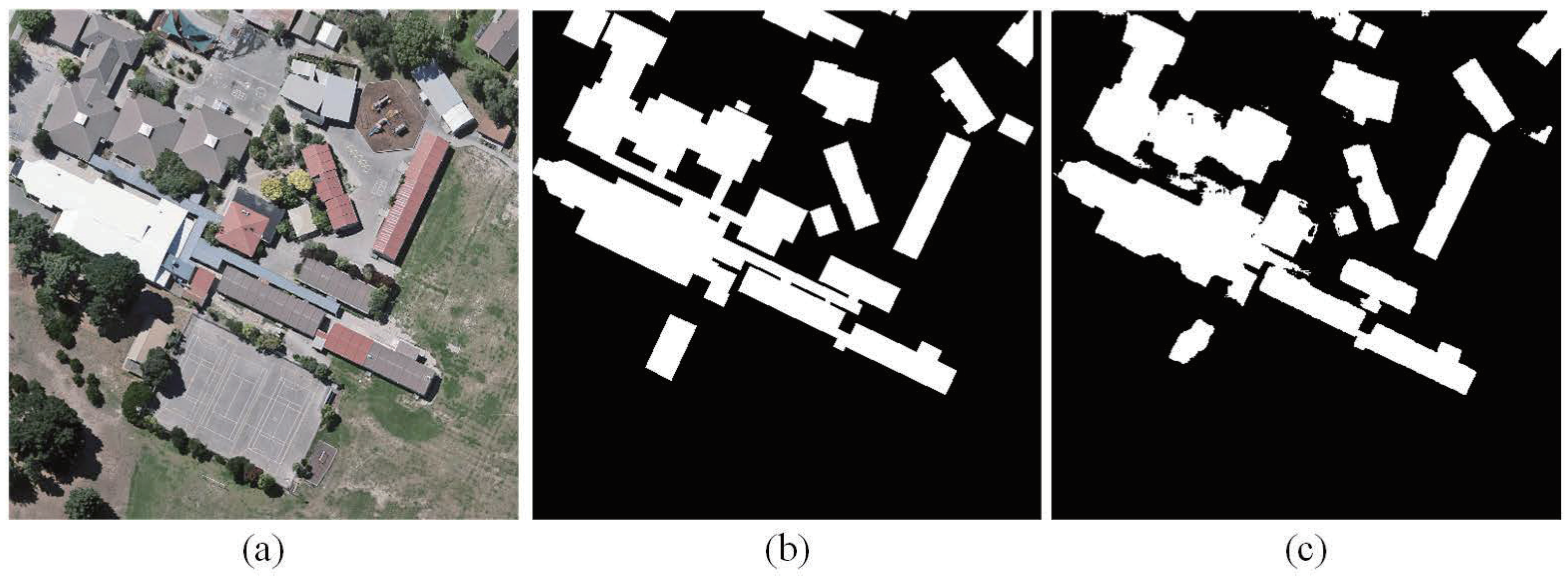
The past few years have witnessed the attainments of FCNs designed for remote sensing imagery segmentation in building extraction. However, owing to the complex shapes, the occlusion of shadows, and the similarity of some artificial features, making segmented buildings maintain their unique morphological characteristics, such as straight lines and right angles, is still a problem that requires immediate resolution [4], as shown in Figure 1.
The morphology of buildings is reflected in their boundaries; thus, some studies have made efforts to predict more accurate boundaries by extracting more boundary information or making use of post-processing techniques. For instance, Sun et al. [28] proposed a method based on the SegNet [17], in which an active contour model is used to refine boundary prediction. Yuan [29] designed a deep FCN that fuses outputs from multiple layers; a signed distance function was designed as the output representation to delineate the boundary information in this work. Shrestha et al. [30] adopted conditional random fields (CRFs) as the post-processing technique to improve the quality of building boundaries in their segmentation results. Xu et al. [31] designed a deep network that takes remote sensing images as input, as well as some hand-crafted features, to extract urban buildings, and employed a guided filter for further optimization. However, methods focusing on acquiring more information about boundaries require more sophisticated structures or use auxiliary data, such as light detection and ranging (LiDAR) [28], normalized differential vegetation index (NDVI), and normalized digital surface model (NDSM) [31], while the post-processing stage usually complicates the methods. To further improve the morphology of buildings, a few studies attempted multi-task frameworks, incorporating segmentation and boundary prediction. For instance, Bischke et al. [32] proposed a multi-task model that preserves the semantic segmentation boundary by optimizing a comprehensive loss, which is composed of the losses of boundary categories and segmentation labels. However, the model training requires considerable time because there is no direct connection between the tasks.
To contrapose this phenomenon, we propose a boundary-assisted learning method for segmenting buildings while keeping the boundary morphology of buildings. On the one hand, an ancillary task, boundary learning, is embedded in parallel with the segmentation task to help maintain the boundaries. On the other hand, a spatial variation fusion (SVF) module is introduced to establish an association between the two tasks, in which way the boundary learning task can obtain a prototype from the segmentation task, while the segmentation task can be constrained by boundary learning, making them promote each other. In addition, to enlarge the receptive fields and decrease the computational cost, separable convolutions [33] with large filters are adopted as the substitute for standard convolutions. Additionally, following the prevalent neural network enhancement technique—the attention mechanism [34]—we introduce the convolutional block attention module (CBAM) [35], which improves visual tasks by combining the channel attention and spatial attention, into our network to boost the model. On this basis, we propose a novel end-to-end FCN framework to accurately extract buildings from remote sensing images. Our experiments exhibit that without using auxiliary data or post-processing, our method achieves superior performance over some SOTA works on two public challenging datasets, known as the WHU Building Dataset [5] and Inria Aerial Image Labeling Dataset [36]. The innovations and contributions of this paper are summarized in the following points.
- A boundary-assisted learning pattern is proposed, with the assistance of which the boundary morphology maintenance of buildings is markedly ameliorated. Moreover, the SVF module combines the segmentation task and boundary learning task so that they can interact with each other, making the network easier to train.
- A new FCN-based architecture is proposed. The utilization of separable convolutions reduces the number of parameters in the model while expanding the receptive fields by using large filters. The introduction of a CBAM plays a role in boosting the model.
2. Methodology
The main purpose of this paper is to explore a means that improves building segmentation by overcoming the inaccurate boundary morphology extracted from remote sensing images. The key idea lies in using the boundary learning task to help maintain buildings’ morphological characteristics and guide the network to optimize the segmentation results. This section begins with an overview of the proposed framework. Then, the significant components, including the SVF module, separable convolution, and CBAM, are elaborated. The loss functions come at the end.
2.1. Overall Framework
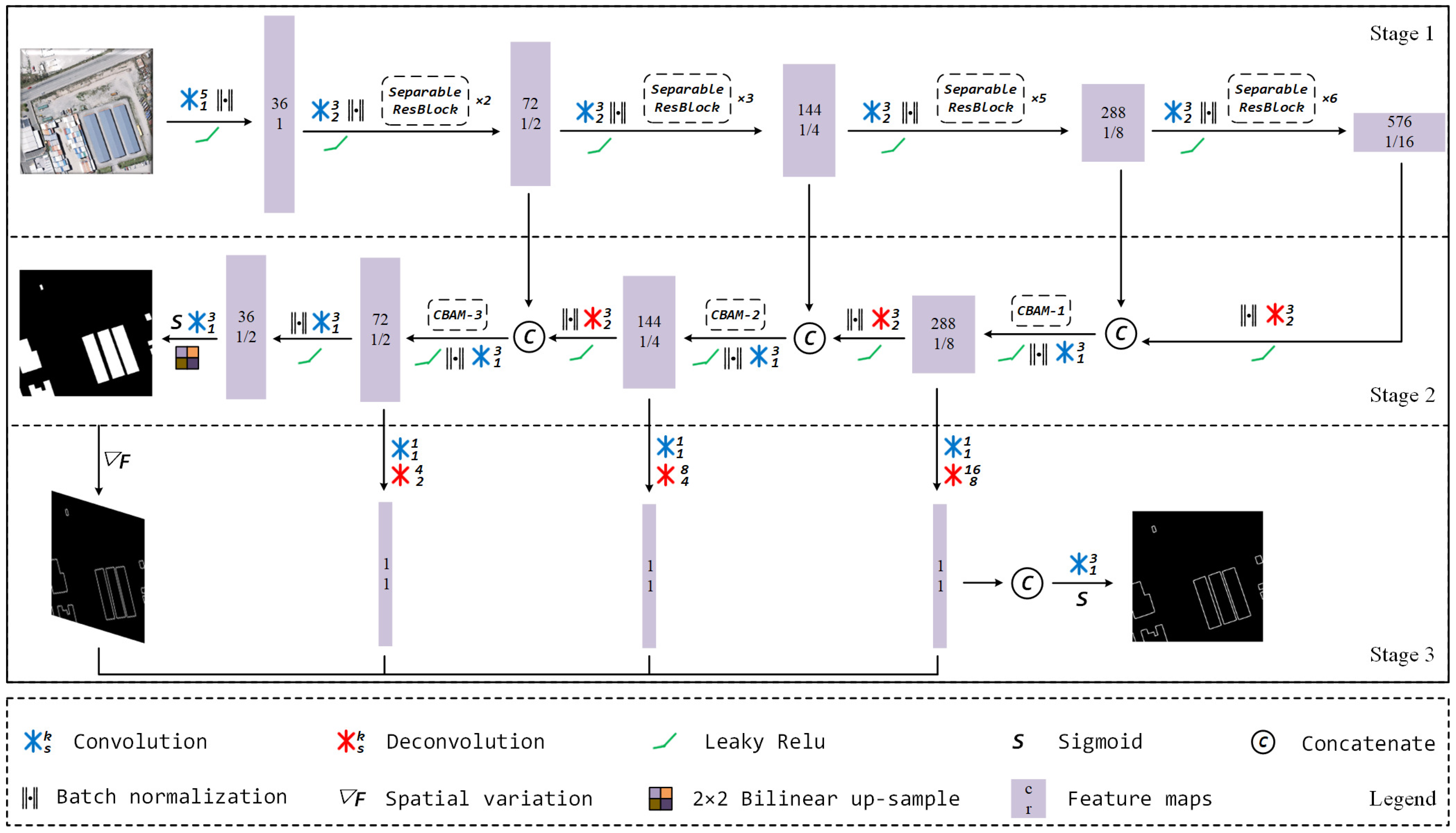
The overall pipeline of our framework is shown in Figure 2, which consists of three stages. In the first stage, an image is fed into a backbone network to generate multi-level semantics. The backbone is modified from the Darknet-53 [37] proposed by YOLOv3 [37]; we replace the original residual block with our “Separable Residual Block” and down-sample the input image four times (in YOLOv3, an input image is down-sampled five times; as excessive down-sampling will lead to information loss of small buildings, we only down-sample the images four times). In the second stage, the feature maps with different spatial resolutions are gradually up-sampled and aggregated to generate the segmentation mask. In the last stage, a preliminary boundary mask is produced after the spatial variation operation is performed; then, the boundary mask is fused with the features extracted from the aggregated semantics to generate the refined boundary. Both the segmentation and boundary masks are generated to compute the loss function in the training phase, but only the former two stages are reserved while testing.
2.2. Significant Modules
As mentioned above, some key components play important roles in our framework. This subsection gives details about them.
2.2.1. Spatial Variation Fusion
After several steps in the second stage, we obtain the segmentation mask probability map . Inspired by the spatial gradient fusion proposed in [38], we modify it and propose the SVF, which easily generates buildings’ semantic boundaries from segmentation masks by deriving spatial variation. We use adaptive pooling to derive the spatial variation :
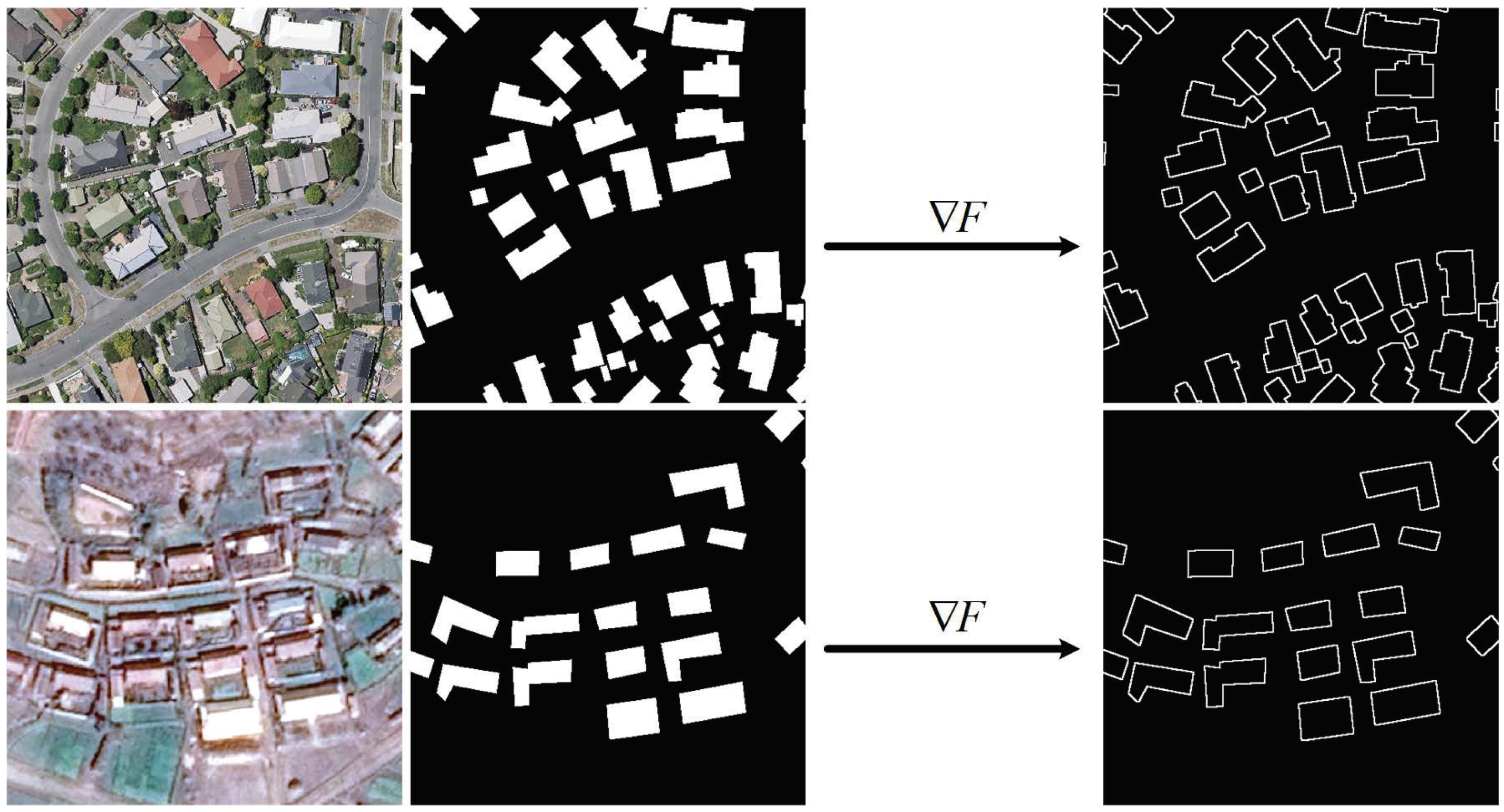
where denotes the location of the mask probability map and refers to the absolute value function. is the max-pooling operation with kernel size k and stride s. k controls the width of the derived boundary; in our framework, we set k to 3 and s to 1. In [38], average pooling is used to produce boundaries. Compared to this, max-pooling can produce more distinct boundaries. Some examples are shown in Figure 3.
Once the boundary mask is produced, it is fused with those single-channel features by concatenation; then, the fusion is again fed into a convolution layer to produce the final boundary mask probability map. The SVF module provides a prototype for boundary learning, while the derived boundary acts as a constraint on segmentation learning. Compared with separate segmentation and boundary generation, the network training becomes easier, as the two tasks can interact with and benefit each other.
2.2.2. Separable Convolution
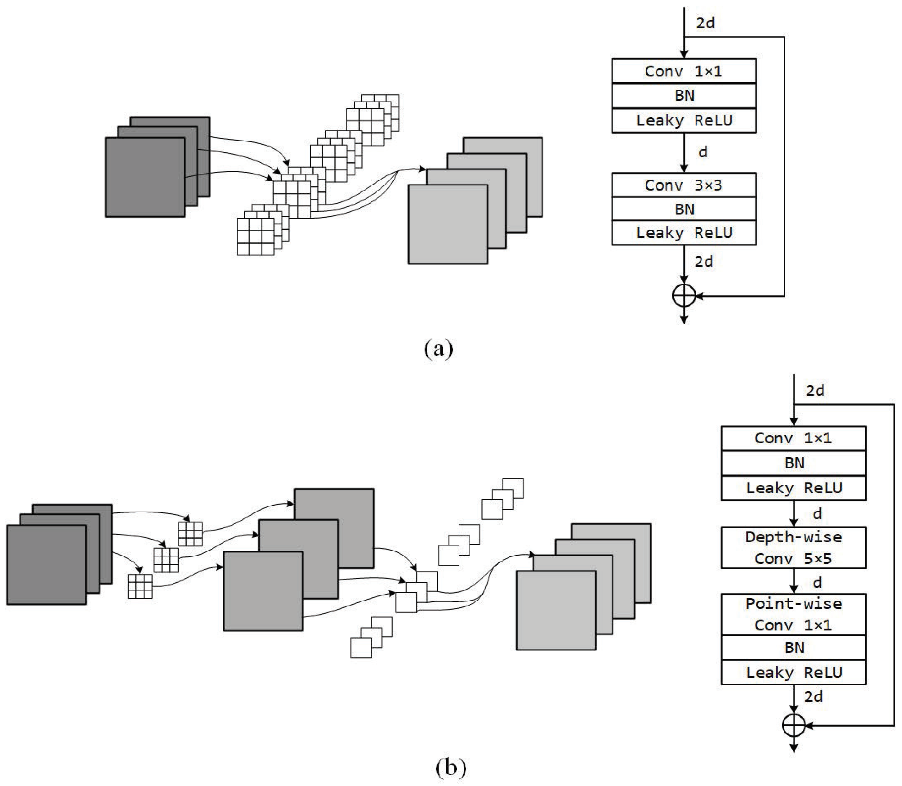
Separable convolution was initially designed for mobile vision applications [34], which aim to achieve equal or even better results with less computation. It performs a depth-wise spatial convolution with a filter size k that acts separately on each input channel, followed by a point-wise convolution with a filter size of 1 that mixes the resulting output channels. Based on separable convolutions, our “Separable Residual Block" is designed as presented in Figure 4.
The “Separable Residual Block" enlarges the receptive field by applying larger filters; meanwhile, the number of parameters is reduced. For example, suppose that the input tensor has channels and the output tensor has channels; then, the number of filter parameters in a standard convolution layer (with a filter size of 3) reaches . However, the number of filter parameters in a separable convolution layer (with a filter size of 5) only reaches , which is dramatically less than that of standard convolution. Thanks to the separable convolution, the number of parameters in our model is reduced by about 18 million.
2.2.3. Convolutional Block Attention Module
Deep neural networks (DNNs) extract hierarchical semantic features, of which the low-level features have poor semantic information but rich spatial location information owing to the small receptive view and large resolution. On the contrary, the high-level features have strong semantic information but weak spatial location information because of the large receptive view and low resolution. Hence, indiscriminate concatenation of features from different levels may cause inconsistencies, which makes networks confused about the attention allocation for high-level features and low-level features [39]. On the other hand, DNNs generate the feature representation of complex objects by collecting different regions of semantic sub-features. However, those sub-features are often spatially affected by similar patterns and noisy backgrounds [40]. Thus, it is necessary to emphasize the important parts and suppress the unimportant parts.
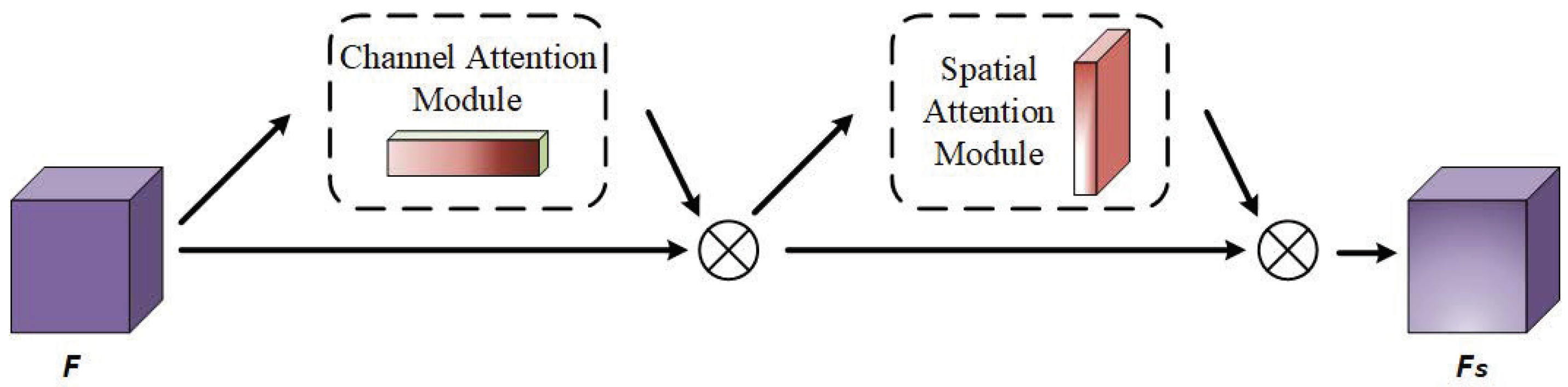
Due to these factors, semantic segmentation based on FCNs is a task that needs to weigh features in the channel dimension and sub-features in the spatial dimension. Therefore, following [35], we introduce the CBAM, which infers attention along the two separate dimensions, into our framework. The CBAM is designed as shown in Figure 5; it is a combination of a channel attention mechanism and spatial attention mechanism.
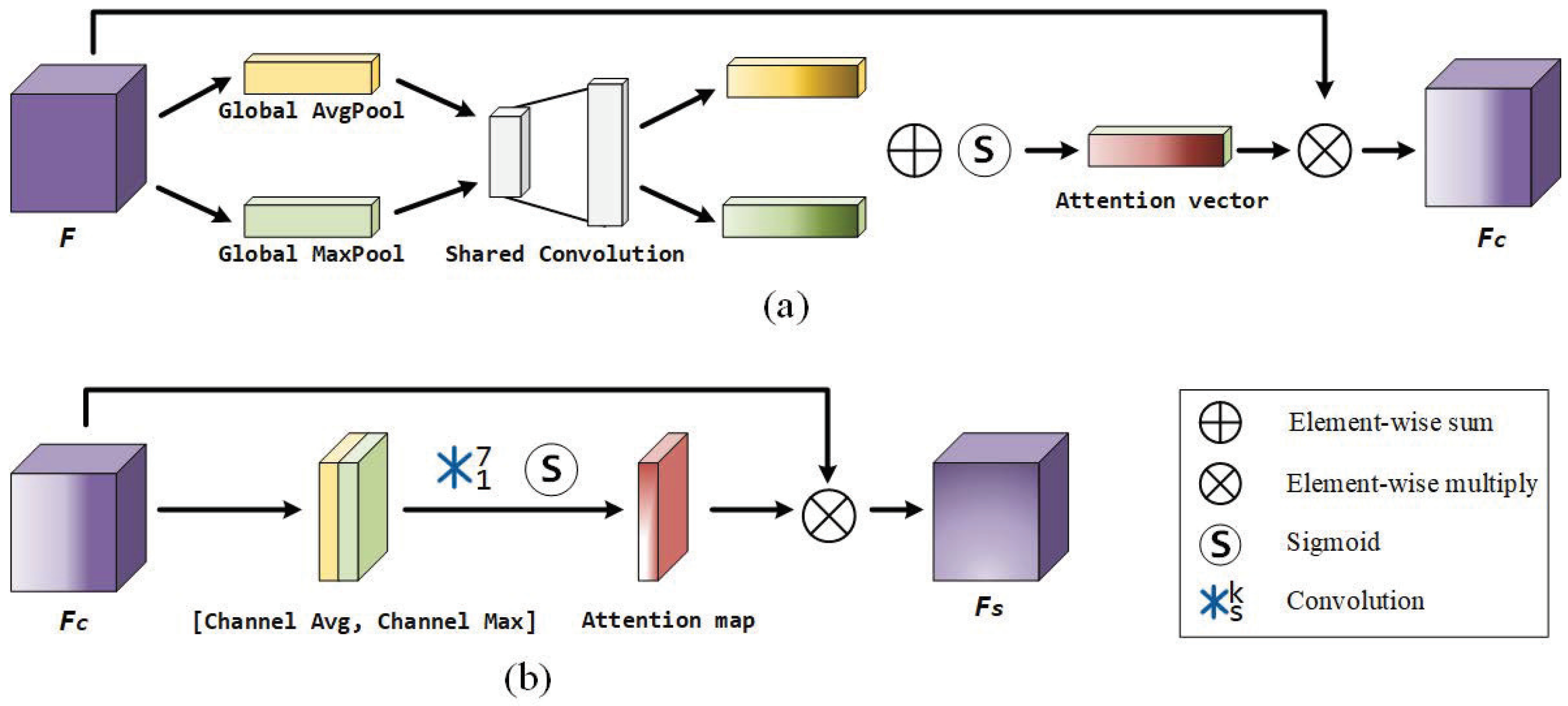
Channel attention (Figure 6a) “tells” the network how to allocate weights for different channels. Given an input feature map, we first squeeze and excite its spatial information [41] by using global average-pooling and global max-pooling, generating two descriptors: and . The former integrates the global information of each channel, while the latter gathers clues about distinctive object features. Then, the descriptors are forwarded to a shared block (consisting of two convolution layers with a filter size of 1) to produce two vectors, which are next merged by an element-wise sum and finally output the 1D attention vector after a sigmoid function is applied. The channel attention is computed as:
Spatial attention (Figure 6b) “tells” the network which regions are informative and should be paid more attention. We first perform average-pooling and max-pooling along the channel axis and concatenate them to generate a descriptor, which helps highlight informative regions [42]. Then, this is fed into a convolution layer with a filter size of 7, which finally produces the 2D attention map with a sigmoid operation. The spatial attention is computed as:
In short, the computation in the CBAM is as follows:
2.3. Loss Functions
As illustrated in Figure 2, two masks are generated from our proposed network—a segmentation probability map and a boundary probability map. Accordingly, we compute two loss functions that correspond to them.
Segmentation loss: For semantic segmentation, the cross-entropy loss is most commonly used, which treats all pixels equally. However, we think that treating backgrounds and buildings equally may make a network less able to recognize buildings in scenes it has never seen before. Therefore, to guide a network to pay more attention to buildings themselves, we propose the foreground-enhanced loss function for this binary classification task:
where and respectively denote the label and predicted probability of pixel , and is the number of pixels in a mini-batch. is the weight assigned to pixel . In our experiments, if pixel belongs to buildings, ; otherwise, . In this way, buildings contribute more to the loss function, making the network focus more on them while training.
Boundary loss: Boundary learning suffers from a higher missing rate, as boundaries are very sparse. To alleviate this impact, we follow [39,43] to define the following class-balanced cross-entropy loss function:
where is the percentage of non-boundary pixels in the ground truth.
In general, a multi-task framework trains all tasks at the same time. However, boundary learning has more difficulties in training from scratch due to the sparsity of boundaries. Therefore, in the early phase of training, we froze the boundary learning task and only trained the segmentation task. When the network can generate a reasonably accurate segmentation mask, we add boundary learning. Thus, the integrated loss function for network optimization in the early phase is:
and the integrated loss function in the later phase is:
where is the weight for balancing the losses (we set it to 2 in our experiments). By this means, a preparatory boundary mask can be provided by the spatial variation to reduce the difficulty of boundary learning.
3. Experiments and Comparisons
This section first introduces the datasets used in the experiments and the experimental implementation details, and then displays the building extraction results and provides qualitative and quantitative comparisons between our methodology and some SOTA FCNs.
3.1. Datasets
The WHU Building Dataset [5] and Inria Aerial Image Labeling Dataset [36] were chosen to evaluate our proposed methodology.
WHU Building Dataset (this dataset is available at https://study.rsgis.whu.edu.cn/pages/download/building_dataset.html): This dataset contains four sub-datasets, from which we selected the aerial imagery dataset and the satellite dataset II. The former covers a surface area of about 450 km in New Zealand, including 8189 tiles of size with a 0.3 m spatial resolution, which were officially divided into a training set (4736 images), validation set (1036 images), and testing set (2416 images). The latter covers 860 km in East Asia with 0.45 m ground resolution. This sub-dataset has 17,388 tiles, among which 13,662 tiles were separated for training and the rest were used for testing.
Inria Aerial Image Labeling Dataset (this dataset is available at https://project.inria.fr/aerialimagelabeling/download/): This dataset has 360 tiles of size with a spatial resolution of 0.3 m, covering 10 cities all over the world. It covers various types of urban buildings, such as sparse courtyards, dense residential areas, and large venues.
Many images from the WHU Building Dataset do not contain any buildings; we performed data scrubbing by excluding such images. The sizes of the images from the Inria Aerial Image Labeling Dataset were too large, so we cropped them into tiles with a stride of 452 pixels to fit in with the GPU’s capacity. Note that the Inria Aerial Image Labeling Dataset only provides ground truth for the training set. Therefore, we followed the official suggestion and selected the first five images of each city from the training set for validation, and the rest were used for training. For both datasets, we adopted random flipping to augment them.
3.2. Implementation Details
All work was done with TensorFlow [44] using Python. For optimization, we adopted an Adam optimizer [43] with a base learning rate of 0.001, which decayed at a rate of 0.9 after every epoch. All models were trained for up to 20 epochs on their corresponding datasets, only saving the best weights. The pixel values of images were rescaled between 0 and 1 before being input into networks, and L2 regularization was introduced in all convolutions with a weight decay of 0.0001 to avoid over-fitting. For the aerial imagery dataset from the WHU Building Dataset, we initialized the convolution kernels with “He initialization” [45]. For the Inria Aerial Image Labeling Dataset, we used the pre-trained weights on the WHU aerial imagery dataset for initialization. Where applicable, we accelerated the training with an NVIDIA GTX 1070Ti GPU. As U-Net [21] had been shown to have obtained nice performance in building extraction [46] and quite a few research works have been inspired by it, we also used re-completion of U-Net as the baseline. It respectively took 430 and 618 min to train our model and U-Net on the WHU Aerial Building Dataset, while training our model and U-Net on the Inria Aerial Image Labeling Dataset took 756 and 1026 min, respectively.
3.3. Results and Comparisons
To demonstrate the superiority of our methodology in building extraction, and especially the maintenance of morphological characteristics of buildings, we simultaneously list the segmentation results of U-Net and our method and focus on comparing the prediction of boundaries. We also quantitatively compare our methodology with some SOTA FCNs by adopting four metrics, that is, precision, recall, F1-score, and intersection-over-union (IoU), to evaluate the performance from multiple perspectives. The precision, recall, and F1-score are respectively defined as:
where TP, FP, and FN represent the pixel numbers of true positives, false positives, and false negatives, respectively. Building pixels are positive while the background pixels are negative. IoU is defined as:
where P denotes the set of pixels predicted as buildings, and P denotes the ground truth set. denotes the function to calculate the number of pixels in the set.
3.3.1. Comparison on the WHU Aerial Building Dataset
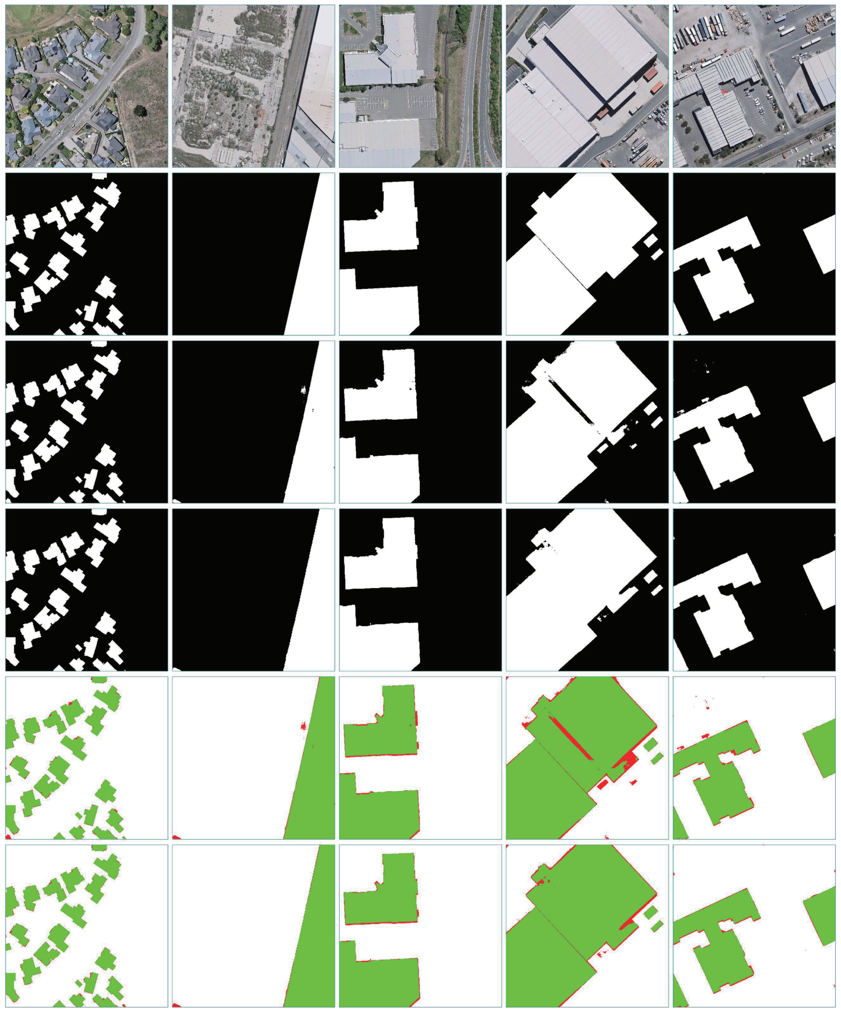
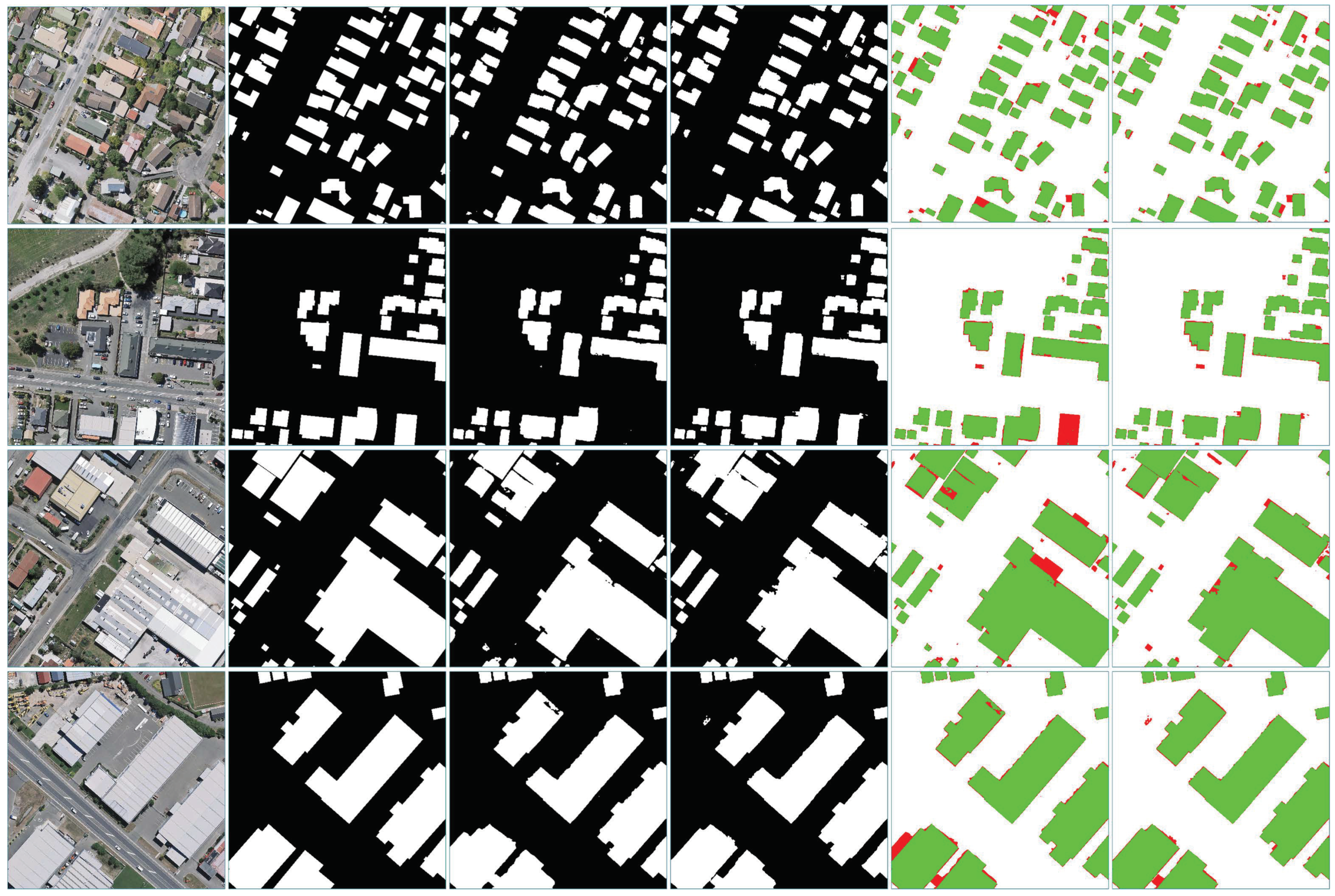
Figure 7 shows the segmentation examples of the WHU Aerial Building Dataset. Through visual inspection, it appears that our method outputs finer segmentation results. There are fewer false positives and clutters in our results. The morphological characteristics of buildings, such as the straight lines and angles, are also better preserved in our results. The last two rows indicate that fewer errors occur in our method, while there exist more wrongly predicted pixels in U-Net, especially around the boundaries.
For further comparison, we compare our framework to several SOTA methods, including the well-known FCNs proposed by the computer vision community, that is, SegNet [17], Deeplab [19], and RefineNet [47], as well as some recent works on remote sensing, that is, SRI-Net [4], CU-Net [46], and SiU-Net [5]. The quantitative comparison is summarized in Table 1. Our method outperforms the baseline (U-Net) by leaps and bounds and ranks first among these methods in terms of recall, F1, and IoU, while only the precision is slightly lower than that of SRI-Net.
3.3.2. Comparison on the Inria Aerial Image Labeling Dataset
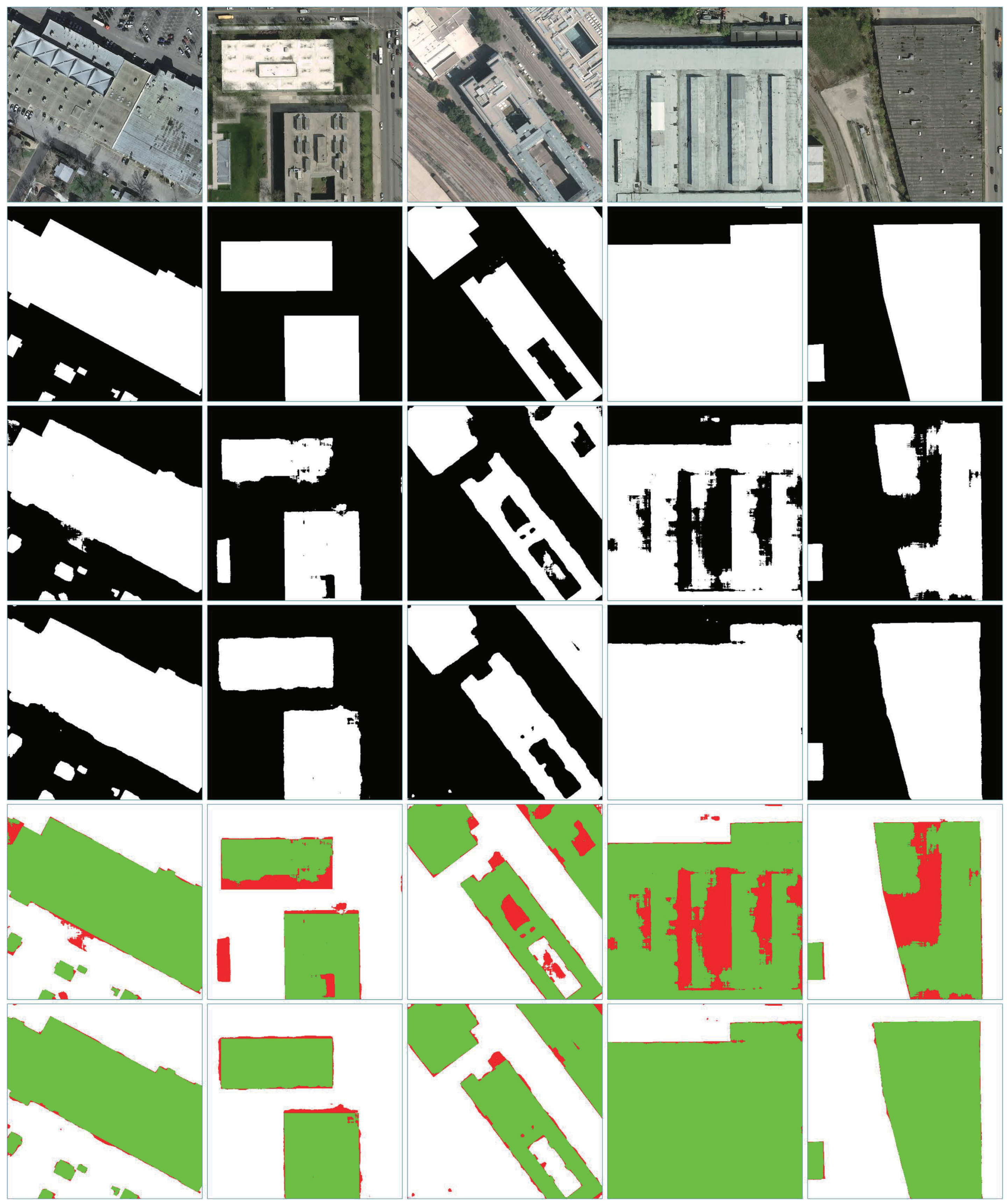
Building extraction examples from the Inria Aerial Image Labeling Dataset are displayed in Figure 8. The results produced by our method contain much fewer errors, and less chaos occurs around the boundaries of buildings. In addition, it is observed that our method outputs more complete buildings compared to U-Net, especially large buildings. This is due to the larger convolution kernels in the separable convolutions and the fact that our network is deeper, which expands the receptive fields of our network, making it capture more context information.
The quantitative comparison with SOTA methods is reported in Table 2. On this dataset, our method also achieves the highest recall, F1, and IoU, far beyond the others. The performance on this aerial dataset is poorer than that on the WHU Aerial Building Dataset; the main reason is that there are more challenging cases, such as higher buildings and shadows. In addition, a few incorrect labels exist in this dataset, as has been illustrated in [5].
In summary, our method achieves the best performance for three indicators, while only the precision is slightly lower. We hypothesize that this could be due to our foreground-enhanced loss function, which highlights buildings more than backgrounds and may cause a few more false positives. Nevertheless, it improves the recall, as fewer building pixels are wrongly predicted as backgrounds. More details are discussed in Section 4.1.
4. Discussion
4.1. Effectiveness of Boundary-Assisted Learning
To verify the effectiveness of boundary-assisted learning in preserving the morphological characteristics of buildings, we designed and trained other kinds of networks that have the same structure as our boundary-assisted learning framework, except that the components for boundary generation are removed. As has been mentioned in Section 3.3.2, our foreground-enhanced loss function may influence the performance; to further discuss this, we trained the networks on the WHU Aerial Building Dataset with different loss functions by changing the weight in Equation (5). In total, we trained eight networks on this dataset—four of them simultaneously learned building extraction and boundary detection, while the other four only learned building extraction. All models were trained for 20 epochs. Table 3 exhibits the performances of networks with different configurations.
The table clearly shows that with the assistance of boundary learning, the network attains better performance on all metrics no matter what value of is set (except for = 3, where the precision is slightly lower, and = 2, where the recall is negligibly lower). Figure 9 also supports this conclusion; the network with the boundary learning task outputs buildings with more complete and explicit boundaries, and fewer pixels are wrongly classified. The weight determines how much attention our network pays to buildings, and the attention grows as increases. In our ablation study, we find that larger leads to lower precision, but brings higher recall most of the time. This is because the more attention is given to buildings, the less likely they are to be classified as backgrounds, but the probability of classifying backgrounds as buildings is increased, too. For a compromise, it is appropriate to set this parameter to 2, which makes the network achieve the best comprehensive performance.
4.2. Analysis of the Attention Module
The attention module, CBAM, plays an important role in boosting our network. We take CBAM-3 as an example and visualize the channel attention as well as the spatial attention to illustrate how it works within the network.
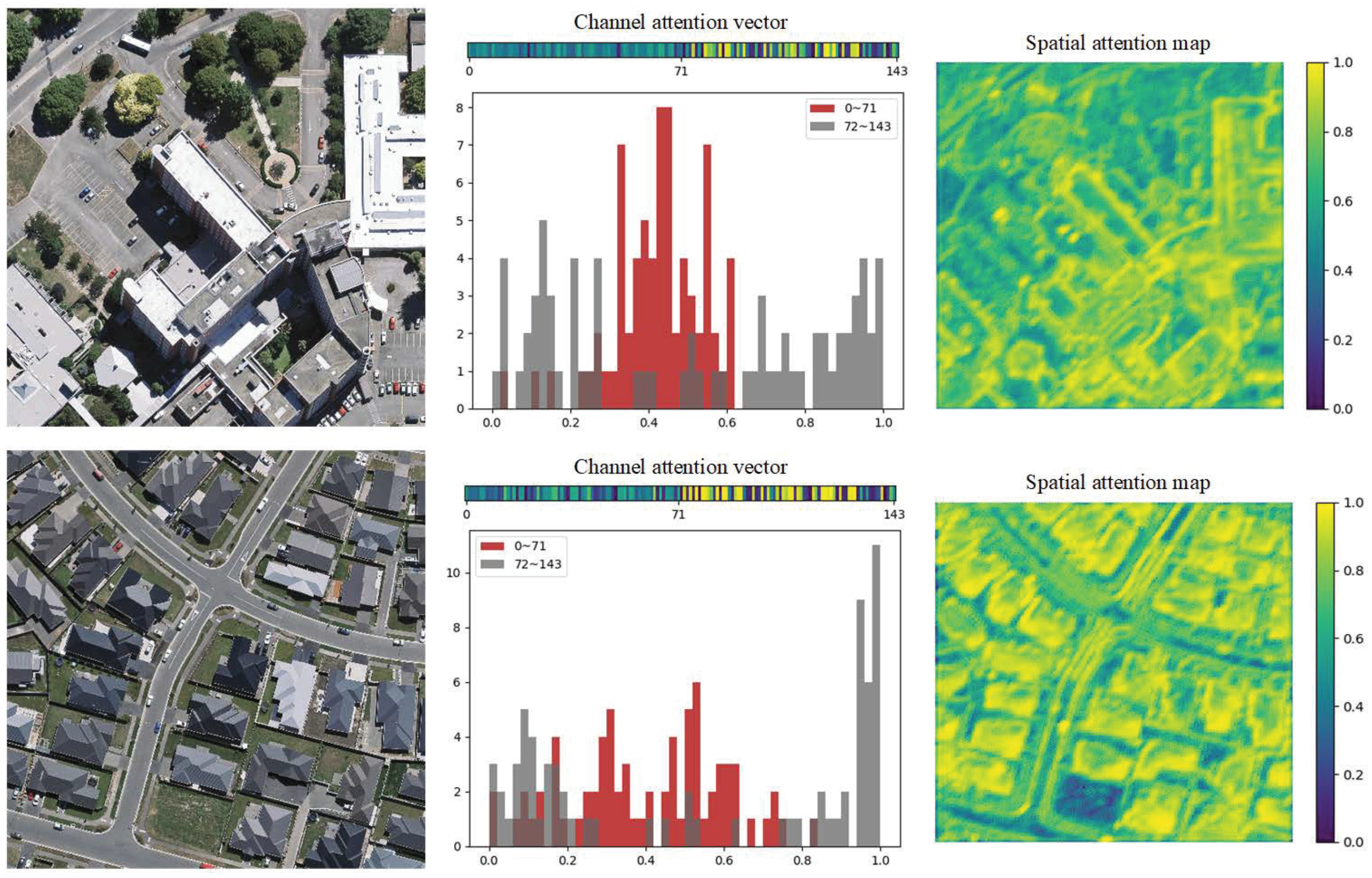
The values of the channel attention vector and spatial attention map are visualized in Figure 10. Channel attention is designed to automatically weigh the channels in the adjacent-level concatenated feature maps, and we analyze it by visualizing the 1D channel attention vector (the former half corresponds to the lower-level feature maps with higher spatial resolution, as well as the latter half for the higher-level one with lower spatial resolution) and drawing the histogram. The vectors indicate that CBAM-3 tends to choose larger weights to act on higher-level feature maps in general, and the tendency becomes obvious as building areas increase. Spatial attention is designed to automatically weigh different regions in feature maps. From the 2D spatial attention map, we can see that the spatial attention successfully guides CBAM-3 to put larger weights on buildings than backgrounds, and the emphasis varies in dealing with different buildings. CBAM-3 focuses more on boundaries when buildings are large and high, while more attention is paid to whole individuals for small and low buildings.
4.3. Evaluation on Satellite Images
The experiments above were performed on aerial image datasets. To explore whether our method also applies to satellite images, we trained our network on the WHU Satellite Building Dataset II, and all training settings were kept the same as for the WHU Aerial Building Dataset. The quantitative evaluation and building extraction results are in Table 4 and Figure 11, respectively.
Compared to the aerial image datasets, the resulting accuracies decreased. Nevertheless, our method is still ahead of the others in the four metrics. The other two methods also perform worse on this dataset, and we argue that the main reason is that those satellite images are poorer in quality and buildings are more blurred, which increases the difficulty of building extraction, as can be observed from the aerial and satellite datasets. However, it is indispensable to further improve current methods for satellite imagery, as they can provide a wider range of Earth observations, which is irreplaceable by aerial imagery.
5. Conclusions
In this paper, a state-of-the-art FCN model for performing building extraction from optical remote sensing images was proposed. The proposed method mainly focuses on three key improvements. (1) A boundary learning task and the spatial variation fusion module are embedded in the semantic segmentation architecture, which helps ameliorate the morphological characteristics of segmented buildings. (2) Separable convolution with a larger kernel is adopted to expand receptive fields, while the number of model parameters is prominently reduced. (3) The convolutional block attention module, which combines channel attention and spatial attention, is utilized to boost the segmentation performance of the model.
Experiments on two challenging aerial image datasets exhibit the superiority of our method. The comparisons demonstrate that our method obtains state-of-the-art building extraction results and ameliorates building boundaries. Moreover, ablation studies give a detailed explanation of the working mechanism of our improvements. The further experiment on satellite images also shows that our method improves the performance of building extraction from satellite images with relatively lower quality. In our future research, we will ulteriorly improve our method.
Author Contributions
Conceptualization, W.J. and S.H.; methodology, S.H.; validation, W.J. and S.H.; formal analysis, S.H.; investigation, W.J.; resources, W.J. and S.H.; data curation, W.J.; writing—original draft preparation, S.H.; writing—review and editing, S.H.; supervision, W.J.; project administration, W.J.; funding acquisition, W.J. All authors have read and agreed to the published version of the manuscript.
Funding
This research was funded by the National Natural Science Foundation of China (Grant Nos. 91638203, 91738302) and the Major Project of High-Resolution Earth Observation Systems (Grant No. 11-Y20A03-9001-16/17).
Institutional Review Board Statement
Not applicable.
Informed Consent Statement
Not applicable.
Data Availability Statement
Codes and models that support this study are available at the private link: https://gitee.com/sheng029/rs-balnet.
Acknowledgments
The authors would like to thank the researchers for providing the wonderful datasets and the developers in the TensorFlow community for their open-source deep learning projects. The authors would also like to express their gratitude to the editors and reviewers for their constructive and helpful comments for the substantial improvement of this paper.
Conflicts of Interest
The authors declare no conflict of interest.
References
- Awrangjeb, M.; Hu, X.Y.; Yang, B.S.; Tian, J.J. Editorial for Special Issue: “Remote Sensing based Building Extraction”. Remote Sens. 2020, 12, 549. [Google Scholar] [CrossRef] [Green Version]
- Rashidian, V.; Baise, L.G.; Koch, M. Detecting Collapsed Buildings after a Natural Hazard on VHR Optical Satellite Imagery Using U-Net Convolutional Neural Networks. In Proceedings of the IEEE International Geoscience and Remote Sensing Symposium, Yokohama, Japan, 28 July–2 August 2019; pp. 9394–9397. [Google Scholar]
- Liu, X.; Liang, X.; Li, X.; Xu, X.; Ou, J. A Future Land Use Simulation Model (FLUS) for Simulating Multiple Land Use Scenarios by Coupling Human and Natural Effects. Landsc. Urban Plan. 2017, 168, 94–116. [Google Scholar] [CrossRef]
- Liu, P.H.; Liu, X.P.; Liu, M.X.; Shi, Q.; Yang, J.X.; Xu, X.C.; Zhang, Y.Y. Building Footprint Extraction from High-Resolution Images via Spatial Residual Inception Convolutional Neural Network. Remote Sens. 2019, 11, 830. [Google Scholar] [CrossRef] [Green Version]
- Ji, S.P.; Wei, S.Q.; Lu, M. Fully Convolutional Networks for Multisource Building Extraction from an Open Aerial and Satellite Imagery Data Set. IEEE Trans. Geosci. Remote Sens. 2019, 57, 574–596. [Google Scholar] [CrossRef]
- Huang, X.; Zhang, L.; Zhu, T. Building Change Detection from Multitemporal High-Resolution Remotely Sensed Images Based on a Morphological Building Index. IEEE J. Sel. Top. Appl. Earth Obs. Remote Sens. 2014, 7, 105–115. [Google Scholar] [CrossRef]
- Wang, D.; Song, W.D. A Method of Building Edge Extraction from Very High Resolution Remote Sensing Images. Environ. Prot. Circ. Econ. 2011, 29, 26–28. [Google Scholar]
- Hu, R.; Huang, X.; Huang, Y. An Enhanced Morphological Building Index for Building Extraction from High-resolution Images. J. Geod. Geoinf. Sci. 2014, 43, 514–520. [Google Scholar]
- Ok, A.O.; Senaras, C.; Yuksel, B. Automated Detection of Arbitrarily Shaped Buildings in Complex Environments from Monocular VHR Optical Satellite Imagery. IEEE Trans. Geosci. Remote Sens. 2013, 51, 1701–1717. [Google Scholar] [CrossRef]
- LeCun, Y.; Bengio, Y.; Hinton, G. Deep Learning. Nature 2015, 521, 436–444. [Google Scholar] [CrossRef]
- Lu, H.; Zhang, Q. Applications of Deep Convolutional Neural Network in Computer Vision. J. Data Acquis. Process. 2016, 31, 1–17. [Google Scholar]
- Krizhevsky, A.; Sutskever, I.; Hinton, G.E. ImageNet Classification with Deep Convolutional Neural Networks. Commun. ACM 2017, 60, 84–90. [Google Scholar] [CrossRef]
- Simonyan, K.; Zisserman, A. Very Deep Convolutional Networks for Large-Scale Image Recognition. arXiv 2014, arXiv:1409.1556. [Google Scholar]
- Szegedy, C.; Liu, W.; Jia, Y.Q.; Sermanet, P.; Reed, S.; Anguelov, D.; Erhan, D.; Vanhoucke, V.; Rabinovich, A. Going Deeper with Convolutions. In Proceedings of the IEEE Conference on Computer Vision and Pattern Recognition, Boston, MA, USA, 7–12 June 2015; pp. 1–9. [Google Scholar]
- Long, J.; Shelhamer, E.; Darrell, T. Fully Convolutional Networks for Semantic Segmentation. In Proceedings of the IEEE Conference on Computer Vision and Pattern Recognition, Boston, MA, USA, 7–12 June 2015; pp. 3431–3440. [Google Scholar]
- Ghosh, S.; Das, N.; Das, I.; Maulik, U. Understanding Deep Learning Techniques for Image Segmentation. ACM Comput. Surv. 2019, 52, 73. [Google Scholar] [CrossRef] [Green Version]
- Badrinarayanan, V.; Kendall, A.; Cipolla, R. SegNet: A Deep Convolutional Encoder-Decoder Architecture for Image Segmentation. IEEE Tran. Pattern anal. Mach. Intell. 2017, 39, 2481–2495. [Google Scholar] [CrossRef] [PubMed]
- Zhao, H.S.; Shi, J.P.; Qi, X.J.; Wang, X.G.; Jia, J.Y. Pyramid Scene Parsing Network. In Proceedings of the IEEE Conference on Computer Vision and Pattern Recognition, Honolulu, Hawaii, USA, 21–26 July 2017; pp. 6230–6239. [Google Scholar]
- Chen, L.C.; Papandreou, G.; Kokkinos, I.; Murphy, K.; Yuille, A.L. DeepLab: Semantic Image Segmentation with Deep Convolutional Nets, Atrous Convolution, and Fully Connected CRFs. IEEE Trans. Pattern Anal. Mach. Intell. 2018, 40, 834–848. [Google Scholar] [CrossRef] [PubMed]
- Pinheiro, P.O.; Lin, T.Y.; Collobert, R.; Dollar, P. Learning to Refine Object Segments. In Proceedings of the European Conference on Computer Vision, Amsterdam, The Netherlands, 8–16 October 2016; pp. 75–91. [Google Scholar]
- Ronneberger, O.; Fischer, P.; Brox, T. U-Net: Convolutional Networks for Biomedical Image Segmentation. In Proceedings of the International Conference on Medical Image Computing and Computer-Assisted Intervention, Munich, Germany, 5–9 October 2015; pp. 234–241. [Google Scholar]
- Everingham, M.; Van Gool, L.; Williams, C.K.I.; Winn, J.; Zisserman, A. The Pascal Visual Object Classes (VOC) Challenge. Int. J. Comput. Vis. 2010, 88, 303–338. [Google Scholar] [CrossRef] [Green Version]
- Lin, T.Y.; Maire, M.; Belongie, S.; Hays, J.; Perona, P.; Ramanan, D.; Dollar, P.; Zitnick, C.L. Microsoft COCO: Common Objects in Context. In Proceedings of the European Conference on Computer Vision, Zurich, Switzerland, 6–12 September 2014; pp. 740–755. [Google Scholar]
- Araujo, T.; Aresta, G.; Castro, E.; Rouco, J.; Aguiar, P.; Eloy, C.; Polonia, A.; Campilho, A. Classification of breast cancer histology images using Convolutional Neural Networks. PLoS ONE 2017, 12, e0177544. [Google Scholar] [CrossRef]
- Volpi, M.; Tuia, D. Dense Semantic Labeling of Subdecimeter Resolution Images with Convolutional Neural Networks. IEEE Trans. Geosci. Remote Sens. 2017, 55, 881–893. [Google Scholar] [CrossRef] [Green Version]
- Yi, Y.N.; Zhang, Z.J.; Zhang, W.C.; Zhang, C.R.; Li, W.D.; Zhao, T. Semantic Segmentation of Urban Buildings from VHR Remote Sensing Imagery Using a Deep Convolutional Neural Network. Remote Sens. 2019, 11, 1774. [Google Scholar] [CrossRef] [Green Version]
- Maggiori, E.; Tarabalka, Y.; Charpiat, G.; Alliez, P. Convolutional Neural Networks for Large-Scale Remote-Sensing Image Classification. IEEE Trans. Geosci. Remote Sens. 2017, 55, 645–657. [Google Scholar] [CrossRef] [Green Version]
- Sun, Y.; Zhang, X.C.; Zhao, X.Y.; Xin, Q.C. Extracting Building Boundaries from High Resolution Optical Images and LiDAR Data by Integrating the Convolutional Neural Network and the Active Contour Model. Remote Sens. 2018, 10, 1459. [Google Scholar] [CrossRef] [Green Version]
- Yuan, J.Y. Learning Building Extraction in Aerial Scenes with Convolutional Networks. IEEE Trans. Pattern Anal. Mach. Intell. 2018, 40, 2793–2798. [Google Scholar] [CrossRef] [PubMed]
- Shrestha, S.; Vanneschi, L. Improved Fully Convolutional Network with Conditional Random Fields for Building Extraction. Remote Sens. 2018, 10, 1135. [Google Scholar] [CrossRef] [Green Version]
- Xu, Y.; Wu, L.; Xie, Z.; Chen, Z. Building Extraction in Very High Resolution Remote Sensing Imagery Using Deep Learning and Guided Filters. Remote Sens. 2018, 10, 144. [Google Scholar] [CrossRef] [Green Version]
- Bischke, B.; Helber, P.; Folz, J.; Borth, D.; Dengel, A. Multi-Task Learning for Segmentation of Building Footprints with Deep Neural Networks. In Proceedings of the IEEE International Conference on Image Processing, Taipei, Taiwan, 22–25 September 2019; pp. 1480–1484. [Google Scholar]
- Howard, A.G.; Zhu, M.L.; Chen, B.; Kalenichenko, D.; Wang, W.J.; Weyand, T.; Andreetto, M.; Adam, H. MobileNets: Efficient Convolutional Neural Networks for Mobile Vision Applications. arXiv 2017, arXiv:1704.04861. [Google Scholar]
- Yi, W.P.; Sebastian, E.; Hinrich, S. Attention-Based Convolutional Neural Network for Machine Comprehension. arXiv 2016, arXiv:1602.04341. [Google Scholar]
- Woo, S.; Park, J.; Lee, J.Y.; Kweon, I.S. CBAM: Convolutional Block Attention Module. arXiv 2018, arXiv:1807.06521. [Google Scholar]
- Maggiori, E.; Tarabalka, Y.; Charpiat, G.; Alliez, P. Can Semantic Labeling Methods Generalize to Any City? The Inria Aerial Image Labeling Benchmark. In Proceedings of the IEEE International Symposium on Geoscience and Remote Sensing, Fort Worth, TX, USA, 23–28 July 2017; pp. 3226–3229. [Google Scholar]
- Redmon, J.; Farhadi, A. YOLOv3: An Incremental Improvement. arXiv 2018, arXiv:1804.02767. [Google Scholar]
- Zhen, M.; Wang, J.; Zhou, L.; Li, S.; Shen, T.; Shang, J.; Fang, T.; Quan, L. Joint Semantic Segmentation and Boundary Detection Using Iterative Pyramid Contexts. In Proceedings of the IEEE Conference on Computer Vision and Pattern Recognition, Seattle, WA, USA, 16–18 June 2020; pp. 13663–13672. [Google Scholar]
- Luo, H.F.; Chen, C.C.; Fang, L.N.; Zhu, X.; Lu, L.J. High-Resolution Aerial Images Semantic Segmentation Using Deep Fully Convolutional Network with Channel Attention Mechanism. IEEE J. Sel. Top. Appl. Earth Observ. Remote Sens. 2019, 12, 3492–3507. [Google Scholar] [CrossRef]
- Li, X.; Hu, X.L.; Yang, J. Spatial Group-wise Enhance: Improving Semantic Feature Learning in Convolutional Networks. arXiv 2019, arXiv:1905.09646. [Google Scholar]
- Hu, J.; Shen, L.; Sun, G. Squeeze-and-excitation Networks. arXiv 2017, arXiv:1709.01507. [Google Scholar]
- Zagoruyko, S.; Komodakis, N. Paying More Attention to Attention: Improving the Performance of Convolutional Neural Networks via Attention Transfer. arXiv 2016, arXiv:1612.03928. [Google Scholar]
- Diederik, P.K.; Jimmy, L.B. Adam: A Method for Stochastic Optimization. arXiv 2017, arXiv:1412.6980. [Google Scholar]
- Abadi, M.; Barham, P.; Chen, J.; Chen, Z.; Davis, A.; Dean, J.; Devin, M.; Ghemawat, S.; Irving, G.; Isard, M.; et al. TensorFlow: A System for Large-Scale Machine Learning. In Proceedings of the USENIX Symposium on Operating Systems Design and Implementation, Savannah, GA, USA, 2–4 November 2016; pp. 265–283. [Google Scholar]
- He, K.M.; Zhang, X.Y.; Ren, S.Q.; Sun, J. Delving Deep into Rectifiers: Surpassing Human-Level Performance on ImageNet Classification. In Proceedings of the IEEE International Conference on Computer Vision, Santiago, Chile, 11–18 December 2015; pp. 1026–1034. [Google Scholar]
- Wu, G.M.; Shao, X.W.; Guo, Z.L.; Chen, Q.; Yuan, W.; Shi, X.D.; Xu, Y.W.; Shibasaki, R. Automatic Building Segmentation of Aerial Imagery Using Multi-Constraint Fully Convolutional Networks. Remote Sens. 2018, 10, 407. [Google Scholar] [CrossRef] [Green Version]
- Lin, G.S.; Milan, A.; Shen, C.H.; Reid, I. RefineNet: Multi-Path Refinement Networks for High-Resolution Semantic Segmentation. In Proceedings of the IEEE Conference on Computer Vision and Pattern Recognition, Honolulu, HI, USA, 21–26 July 2017; pp. 5168–5177. [Google Scholar]
Figure 1.
(a) The original image, (b) the ground truth, and (c) the prediction by U-Net [21]. There exist clutters around the boundaries, and some buildings are incomplete. The straight lines and right angles of some buildings are not well preserved.
Figure 1.
(a) The original image, (b) the ground truth, and (c) the prediction by U-Net [21]. There exist clutters around the boundaries, and some buildings are incomplete. The straight lines and right angles of some buildings are not well preserved.

Figure 2.
The overall architecture of our framework. The first stage produces multi-level semantics with different spatial resolutions (1/2, 1/4, and 1/16 of the input size, respectively). The second stage parses them to the segmentation mask. The last stage generates the boundary mask. While testing, only the former two stages are reserved.

Figure 3.
Some visualization examples for the segmentation mask and inferred semantic boundary through spatial variation derivation.
Figure 3.
Some visualization examples for the segmentation mask and inferred semantic boundary through spatial variation derivation.

Figure 4.
Convolution and residual blocks. (a) denotes the standard convolution and residual block used in YOLOv3 [37], and (b) denotes the separable convolution and our advanced “Separable Residual Block”.
Figure 4.
Convolution and residual blocks. (a) denotes the standard convolution and residual block used in YOLOv3 [37], and (b) denotes the separable convolution and our advanced “Separable Residual Block”.

Figure 5.
The structure of the convolutional block attention module (CBAM). It is composed of two sub-modules.
Figure 5.
The structure of the convolutional block attention module (CBAM). It is composed of two sub-modules.

Figure 6.
The channel attention mechanism and spatial attention mechanism. (a) and (b) respectively denote the channel attention module and spatial attention module.
Figure 6.
The channel attention mechanism and spatial attention mechanism. (a) and (b) respectively denote the channel attention module and spatial attention module.

Figure 7.
Examples of building extraction results produced by our method and U-Net on the WHU Aerial Building Dataset. The first two rows are aerial images and the ground truth. The predictions by U-Net and our method are in row 3 and row 4, respectively. The last two rows show the errors (wrongly predicted pixels are marked in red) of U-Net and our method, respectively.

Figure 8.
Examples of building extraction results produced by our method and U-Net on the Inria Aerial Image Labeling Dataset. The first two rows are aerial images and the ground truth. The predictions by U-Net and our method are in row 3 and row 4, respectively. The last two rows show the errors (wrongly predicted pixels are marked in red) of U-Net and our method, respectively.

Figure 9.
Examples of building extraction produced by “w/B” and “B”. From left to right: aerial images, labels, predictions of “w/B”, predictions of “B”, errors of “w/B”, and errors of “B”. The weight is set to 2.
Figure 9.
Examples of building extraction produced by “w/B” and “B”. From left to right: aerial images, labels, predictions of “w/B”, predictions of “B”, errors of “w/B”, and errors of “B”. The weight is set to 2.

Figure 10.
Visualization examples of the attention mechanism (best view in colors). The numbers 0–71 denote the feature map channels from the lower level, while 72–143 denote that from the higher level. The CBAM guides the network to pay different amounts of attention to different feature map channels and regions while addressing different images.

Figure 11.
Examples of building extraction results on the WHU Satellite Building Dataset II. From left to right: satellite images, labels, predictions, and errors.
Figure 11.
Examples of building extraction results on the WHU Satellite Building Dataset II. From left to right: satellite images, labels, predictions, and errors.


Table 1.
Quantitative comparison (%) of several state-of-the-art (SOTA) methods used on the WHU Aerial Building Dataset (the highest values are underlined). The first three methods and SRI-Net were implemented by [4], SiU-Net [5] is the official method provided by the dataset, and the others were implemented by [5].
| Method | Precision | Recall | F1 | IoU |
|---|---|---|---|---|
| SegNet | 92.1 | 89.9 | 91.0 | 85.8 |
| Deeplab | 94.3 | 92.2 | 93.2 | 87.3 |
| RefineNet | 93.7 | 92.3 | 93.0 | 86.9 |
| SRI-Net | 95.2 | 93.3 | 94.2 | 89.1 |
| CU-Net | 94.6 | 91.7 | 93.1 | 87.1 |
| SiU-Net | 93.8 | 93.9 | 93.8 | 88.4 |
| U-Net | 91.4 | 94.5 | 92.9 | 86.8 |
| Ours | 95.1 | 94.9 | 95.0 | 90.5 |
Table 2.
Quantitative comparison (%) with several SOTA methods on the Inria Aerial Image Labeling Dataset (the highest values are underlined). The first three methods and SRI-Net were implemented by [4], who cropped the Inria aerial images to tiles of pixels.
Table 2.
Quantitative comparison (%) with several SOTA methods on the Inria Aerial Image Labeling Dataset (the highest values are underlined). The first three methods and SRI-Net were implemented by [4], who cropped the Inria aerial images to tiles of pixels.
| Method | Precision | Recall | F1 | IoU |
|---|---|---|---|---|
| SegNet | 79.6 | 75.4 | 77.4 | 63.2 |
| Deeplab | 84.9 | 81.3 | 83.1 | 71.1 |
| RefineNet | 86.4 | 80.3 | 82.7 | 70.1 |
| SRI-Net | 85.8 | 81.5 | 83.4 | 71.8 |
| U-Net | 83.1 | 81.1 | 82.1 | 69.7 |
| Ours | 83.5 | 91.1 | 87.1 | 77.2 |
Table 3.
The performance comparison (%) of networks with different architectures and loss functions on the WHU Aerial Building Dataset. “w/B” denotes networks that only learn building extraction, and “B” denotes networks that simultaneously learn building extraction and boundary detection.
Table 3.
The performance comparison (%) of networks with different architectures and loss functions on the WHU Aerial Building Dataset. “w/B” denotes networks that only learn building extraction, and “B” denotes networks that simultaneously learn building extraction and boundary detection.
| Precision | Recall | F1 | IoU | |||||
|---|---|---|---|---|---|---|---|---|
| w/B | B | w/B | B | w/B | B | w/B | B | |
| 1 | 94.8 | 95.5 | 93.9 | 94.5 | 94.3 | 95.0 | 89.3 | 90.4 |
| 2 | 93.9 | 95.1 | 95.0 | 94.9 | 94.4 | 95.0 | 89.4 | 90.5 |
| 3 | 92.8 | 92.0 | 94.3 | 96.3 | 93.5 | 94.1 | 87.8 | 88.9 |
| 5 | 89.6 | 90.2 | 96.8 | 96.9 | 93.1 | 93.4 | 87.0 | 87.7 |
Table 4.
Quantitative evaluation (%) and comparison on the WHU Satellite Building Dataset II (SiU-Net [5] is the official method provided by this dataset; the highest values are underlined).
Table 4.
Quantitative evaluation (%) and comparison on the WHU Satellite Building Dataset II (SiU-Net [5] is the official method provided by this dataset; the highest values are underlined).
| Method | Precision | Recall | F1 | IoU |
|---|---|---|---|---|
| U-Net | 76.7 | 74.5 | 75.6 | 60.7 |
| SiU-Net | 72.5 | 79.6 | 75.9 | 61.1 |
| Ours | 79.5 | 82.3 | 80.9 | 67.9 |
Publisher’s Note: MDPI stays neutral with regard to jurisdictional claims in published maps and institutional affiliations. |
© 2021 by the authors. Licensee MDPI, Basel, Switzerland. This article is an open access article distributed under the terms and conditions of the Creative Commons Attribution (CC BY) license (http://creativecommons.org/licenses/by/4.0/).
Share and Cite
MDPI and ACS Style
He, S.; Jiang, W. Boundary-Assisted Learning for Building Extraction from Optical Remote Sensing Imagery. Remote Sens. 2021, 13, 760. https://doi.org/10.3390/rs13040760
AMA Style
He S, Jiang W. Boundary-Assisted Learning for Building Extraction from Optical Remote Sensing Imagery. Remote Sensing. 2021; 13(4):760. https://doi.org/10.3390/rs13040760
Chicago/Turabian StyleHe, Sheng, and Wanshou Jiang. 2021. "Boundary-Assisted Learning for Building Extraction from Optical Remote Sensing Imagery" Remote Sensing 13, no. 4: 760. https://doi.org/10.3390/rs13040760
Note that from the first issue of 2016, this journal uses article numbers instead of page numbers. See further details here.