Fully Automated Detection of Supraglacial Lake Area for Northeast Greenland Using Sentinel-2 Time-Series
by
 , , and
Philipp Hochreuther
1,* ,
,
Niklas Neckel
2,
Nathalie Reimann
1,
Angelika Humbert
2,3 and
Matthias Braun
1 1
Institute of Geography, Friedrich-Alexander University Erlangen-Nürnberg, 91058 Erlangen, Germany
2
Helmholtz Centre for Polar and Marine Research, Alfred Wegener Institute, 27570 Bremerhaven, Germany
3
Department of Geosciences, University of Bremen, 28359 Bremen, Germany
*
Author to whom correspondence should be addressed.
Remote Sens. 2021, 13(2), 205; https://doi.org/10.3390/rs13020205
Submission received: 7 December 2020
/
Revised: 31 December 2020
/
Accepted: 1 January 2021
/
Published: 8 January 2021
Abstract
:The usability of multispectral satellite data for detecting and monitoring supraglacial meltwater ponds has been demonstrated for western Greenland. For a multitemporal analysis of large regions or entire Greenland, largely automated processing routines are required. Here, we present a sequence of algorithms that allow for an automated Sentinel-2 data search, download, processing, and generation of a consistent and dense melt pond area time-series based on open-source software. We test our approach for a ~82,000 km2 area at the 79 °N Glacier (Nioghalvfjerdsbrae) in northeast Greenland, covering the years 2016, 2017, 2018 and 2019. Our lake detection is based on the ratio of the blue and red visible bands using a minimum threshold. To remove false classification caused by the similar spectra of shadow and water on ice, we implement a shadow model to mask out topographically induced artifacts. We identified 880 individual lakes, traceable over 479 time-steps throughout 2016–2019, with an average size of 64,212 m2. Of the four years, 2019 had the most extensive lake area coverage with a maximum of 333 km2 and a maximum individual lake size of 30 km2. With 1.5 days average observation interval, our time-series allows for a comparison with climate data of daily resolution, enabling a better understanding of short-term climate-glacier feedbacks.
1. Introduction
The accelerating ice loss of the Greenland Ice Sheet, especially during the last decade, has been detected in multiple studies and marked the island as a focus of cryospheric, atmospheric and oceanographic research and modeling [1,2,3]. Supraglacial lakes (SGL) characterize the melt area (upstream the grounding line) of several marine-terminating outlet glaciers [4,5]. SGL influence surface melts through lowering the albedo and can affect ice flow velocities after drainage through reducing basal friction [6,7]. Furthermore, the variability of their spatial extent and coverage has been reported to be linked to regional variations of surface temperatures [4]. For the monitoring of these lakes, multispectral satellite-based remote sensing is a reasonable method, as the areas that need to be monitored are vast, and the SGL, except in the case of cloud cover, can be mapped efficiently using single bands or band combinations. As a consequence, in (south-) west Greenland, numerous studies have related spectral information from different sensors (Table 1) to either in situ measurements of lake depths or sinks derived from digital elevation models (DEMs, [8] and references therein).
Though potentially, there are numerous multispectral sensors available, each technique has merits and flaws, mostly regarding resolution, acquisition frequency, spatial coverage and accessibility (Table 1). Thus, in most studies, a compromise must be made. Sentinel-2 A/B (S-2), with its multispectral instrument (MSI), combines the advantages of the sensors above, having 10 m resolution with less than two days revisit interval for polar areas available at no charge. Thus, even though data are only available since the launch of S-2 A in June 2015, it offers an unprecedented chance to detect and monitor SGL in remote and polar regions at high spatial and temporal resolution. Until now, there are only very few studies that employ S-2 for the detection of supraglacial lakes or rivers [9,10].
A common problem hindering an automated detection of SGL with multispectral sensors over Greenland is clouds. This problem is enhanced by the gap between the revisits of the satellite, especially for the Landsat series, as, if one or more acquisitions are unusable, large gaps in the time-series can occur. Furthermore, standard cloud detection products (Sen2cor, fmask) are optimized for vegetated and built-up areas but have deficiencies in reliably separating ice and snow from clouds over polar areas (see Section 3 and Section 4). Thus, checking of data must be done manually, especially if only parts of the area of interest (AOI) are cloud-covered. While for small areas and/or single days, this is a valid procedure, processing of large areas or longer time-series requires a different solution.
The majority of all SGL detection studies for Greenland were carried out in western Greenland, in the region between Disco Bay (~70°N) and Kangerlussuaq (~67°N) (Figure 1), mainly because (a) of the number of SGL that appear here on the lower ice sheet each year, and (b) this part of Greenland is comparatively well accessible and logistics for ground-truthing of, e.g., lake depth is available [11]. Only very few studies were conducted outside this area, e.g., at Petermann Glacier or northwest Greenland (Figure 1). The east coast of Greenland, and especially the northeastern part, has been subject to only one previous high-resolution multispectral study on SGLs [12]. Only one study using MODIS in 2009 covered the melting seasons 2002–2008 and found a maximum seasonal total lake area of 149.6 km2 [13]. Contrasting to the spatial distribution of studies, northeast Greenland is expected to show the greatest inland expansion of SGL in the coming decades [14]. However, continuous monitoring of SGLs is currently lacking.
With this study, we aim to:
- develop a method that allows for continuous and automated detection of SGLs using solely open-source software;
- provide an up-to-date and high-resolution dataset of SGLs for the Northeast Greenland Ice Stream (NEGIS) outlet glaciers, Nioghalvfjerdsbrae and Zachariæ Isstrøm;
- detect characteristic features of melt pond development in northeast Greenland.
2. Materials and Methods
2.1. Area of Interest
The study region of ~82,000 km2 covers the ice sheet upstream the grounding lines of Nioghalvfjerdsbrae (hereafter 79°N Glacier) and Zachariæ Isstrøm between sea level and ~1500 m a.s.l. The extent of ~150 km inland and, due to the widening of the glacier bed into the ice sheet, ~300 km latitudinal, is covered by ten S-2 tiles (Figure 1). The glacial dynamics of the region have been strongly affected by climate warming, e.g., through the collapse of the floating tongue of Zachariæ Isstrøm in 2012 [31]. In contrast to the more southern Greenland east coast, the catchment of NEGIS shows comparatively gentle slopes, which enable the retention of surface meltwater upon the ice and thus the formation of numerous lakes during the melting season.
2.2. Preprocessing of Sentinel-2 Data, Screening, and Preselection
In total, 39,919 S-2 A/B level-1C (L1C) scenes were downloaded from the Google cloud storage using the Google Cloud SDK repository for Ubuntu (https://cloud.google.com/storage/docs/public-datasets/sentinel-2?hL=de, last accessed 24 May 2020). We requested a minimum data coverage of 90%, which was checked using quickviews, and a full set of 10 granules; all data with higher no-data content and no full coverage were removed. For all remaining days, the granules of bands 2 (blue, 0.460–0.520 µm), 3 (green, 0.534–0.582 µm) and 4 (red, 0.655–0.684 µm) were first reprojected to EPSG 3413 and then separately merged. In order to circumvent misclassifications in the next steps, we removed the areas not covered by the glacier (rock, ocean) using the GIMP land classification map [30], which was edited manually using two true-color S-2 A images from July 2016 to accurately delineate the up-to-date ice margin.
S-2 data are available between mid of March and mid of September for northeast Greenland, though the first and last day of the year (DOY) for which a complete set of images was found varies between DOY 82–93, and 262–263, respectively. Though S-2 A was launched in June 2015, the data coverage and quality for its first year were found too low to facilitate a meaningful time-series analysis. With S-2 B starting in March 2017, the year 2016 had the lowest data coverage among the 2016–2019 period, while the highest number of complete scenes was found for 2019 (Table 2). On average, 120 complete scene sets were found per year, resulting in an average interval of 1.49 days.
2.3. Water Area Delineation
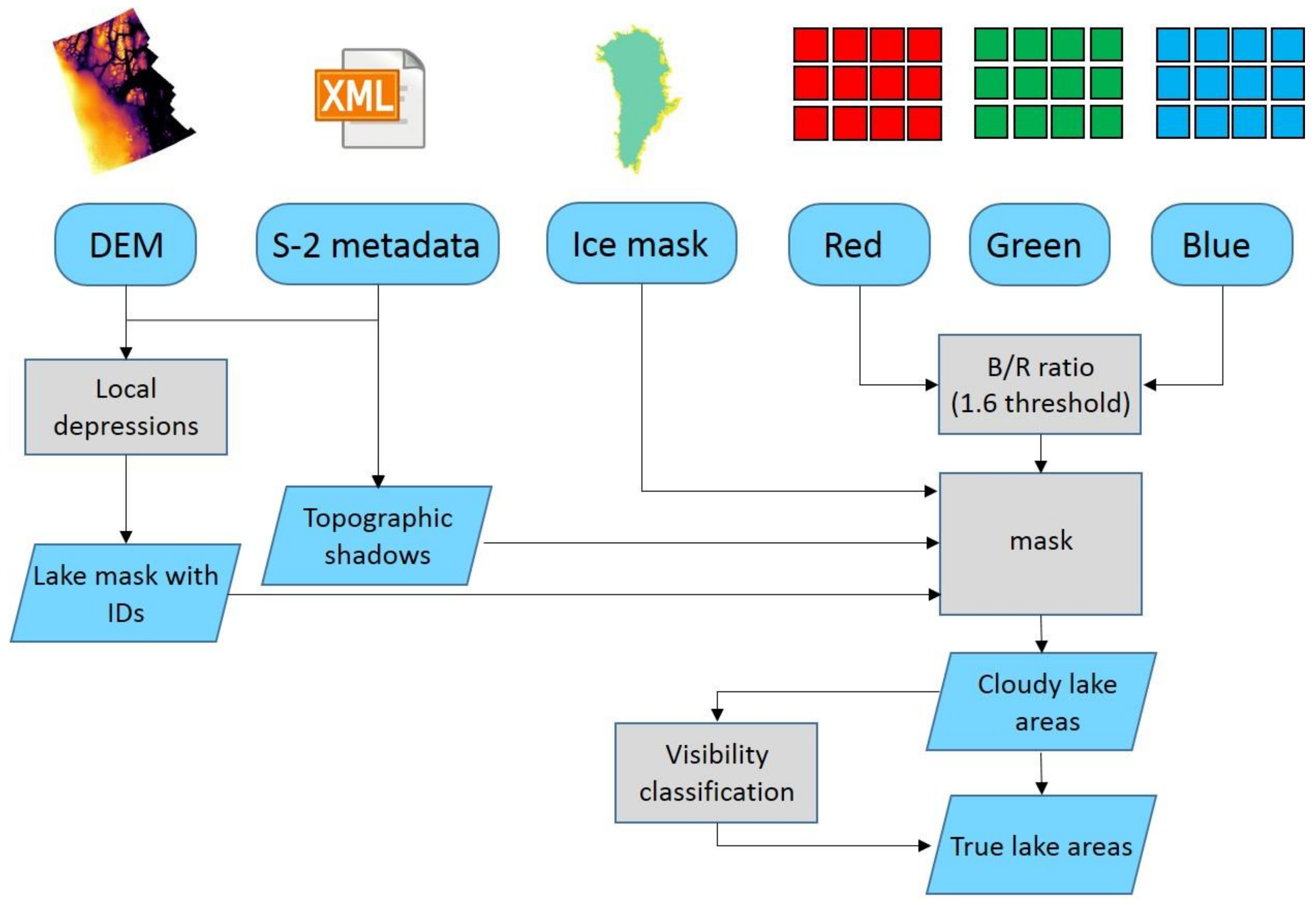
The complete algorithm developed to detect and calculate lake areas is summarized in Figure 2. Following Pope and colleagues (2016), we applied a static band ratio of the blue (band 2) and red (band 4) top-of-atmosphere reflectance, as successfully used in previous studies for Landsat and MODIS [4,11,24,32]. We also tested the normalized difference water index (NDWI) as used by Williamson and colleagues [9], but continued with the band ratio due to comparable results but significantly less computation time (see Section 4.1.1). For determination of the threshold which delineates ice/slush from water, we empirically tested values between 1.0 and 2.4 in 0.2 steps and compared the resulting masks to true color images for several dates and found >1.6 as the best fit. Subsequently, for all dates, the B/R ratio was calculated, and the threshold of 1.6 applied, resulting in binary water masks with 0 as ice and 1 as water.
2.4. Postprocessing
The removal of noise is the main aim of postprocessing. Four main sources of noise were identified and addressed:
- Water-soaked snow and meltwater channels;
- Lake ice on SGLs, resulting in “donut lakes” [33];
- Topographic shadows misclassified as water;
- Clouds and cloud shadows, covering lakes or being classified as water areas.
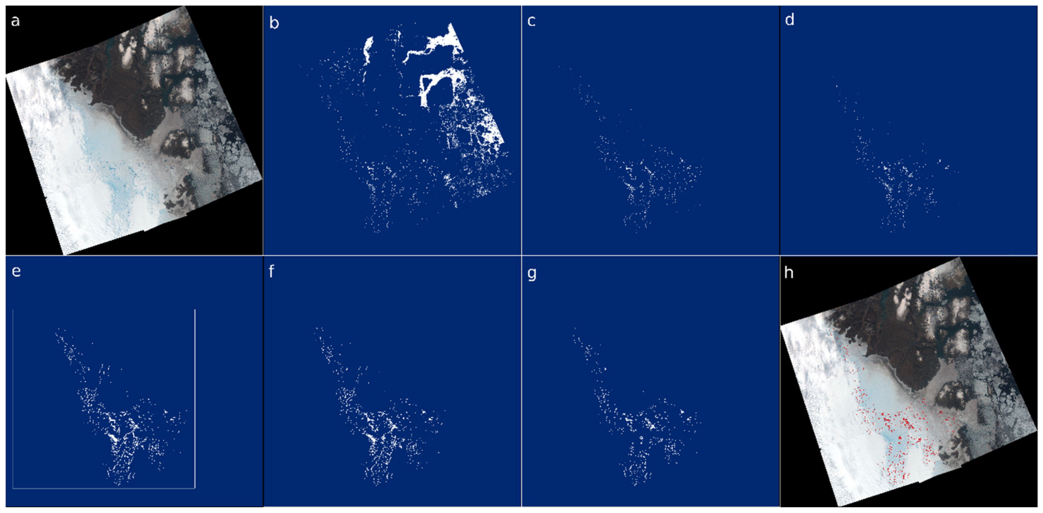
The effects of the subsequent steps are exemplarily visualized in Figure 3.
2.4.1. Area Reduction
To allow for faster computation, the binary B/R ratio images were first cropped to the ablation area of 79 N. We define the eastern extent by the glacier outline mask (Section 2.2) combined with the grounding line based on ERS-II SAR [34], and the northern and southern boundaries are delimited by the extent of S-2 granules 26XMQ, and 26XMN/26XNN, respectively. The western extent is limited by the surface mass balance equaling zero, calculated using the regional atmospheric climate model version 2.3 (RACMO2.3) [35].
2.4.2. Topographic Shadow Masks
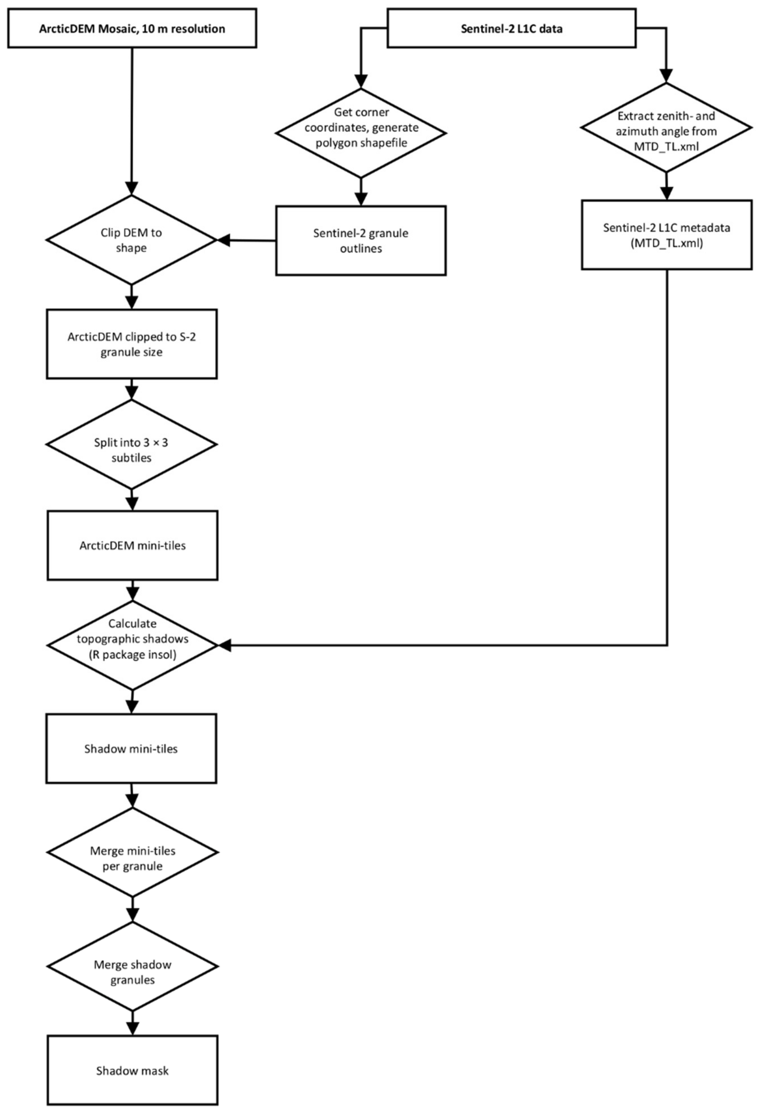
Especially in spring and autumn (March–May and September/October), due to the low solar elevation angles of >70° from nadir (Figure A1), large shadows are cast on the ice even though small topographic features such as hills, crevasses or seracs. These shadows have a similar spectral blue-red ratio as water and thus are commonly misclassified using the band ratio method [36]. To correct for these misclassifications, we applied a topographic shadow model using the R package “insol” [37] (Figure A2). We used the ArcticDEM with 10 m resolution to fit the resolution of the S-2 derived water mask. Additionally, the sun position (elevation and azimuth) is retrieved for the exact time of image acquisition from the S-2 metadata. As the model requires substantial memory resources, we divided the DEM first into parts covering each granule, and subsequently split each part into nine (3 × 3) equal pieces and calculated the topographic shadows for each part and day separately. Afterward, the small binary shadow masks were merged again to cover the whole AOI. A random sample of 30 of the resulting binary masks from all years and seasons was compared visually to the natural-color image of the respective date to ensure fitting and quality of the calculation; afterward, the shadow mask was subtracted from the previous water mask.
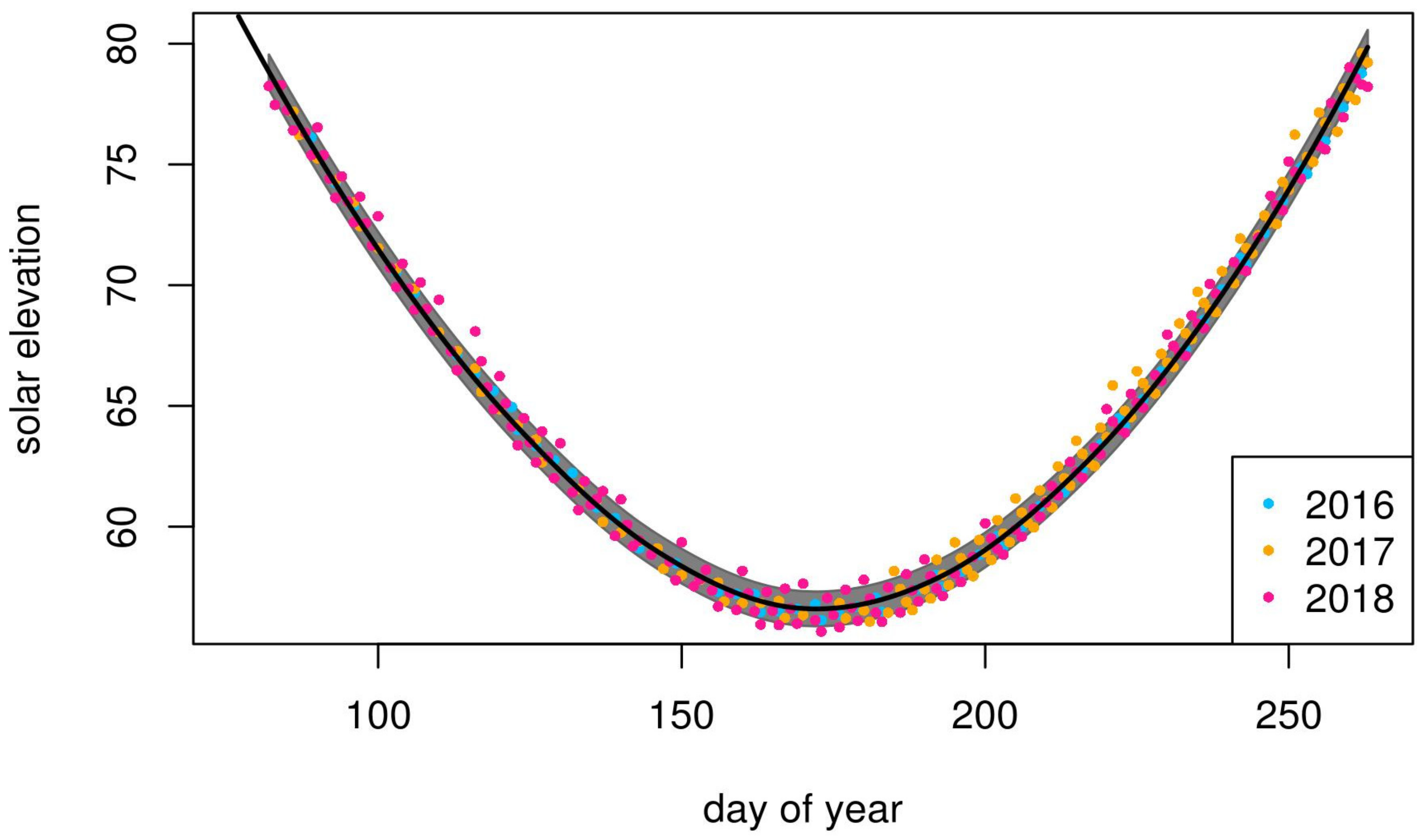
As the computation of shadow masks is computationally expensive, we developed a general function for the sun’s elevation and azimuth based on S-2 metadata of 2016, 2017 and 2018 to speed up this process. Validity-tested using the 2019 data, the pre-computed shadow masks serve as a look-up table for future processing. To achieve that, we calculated the mean for both parameters for each available acquisition and used a local regression to predict the missing values and smoothen the existing ones in order to achieve an idealized solar cycle (Figure A1). These estimated values of elevation- and azimuth angles were used for the shadow calculations of 2019 and are also implemented in the continuously running algorithm.
2.4.3. De-Noising and Filling
The shadow-corrected rasters were subsequently filtered using the sieve tool embedded in the geospatial data abstraction library (GDAL, [38]). To find the lowest possible pixel threshold to retain the maximum information and remove the maximum percentage of noise, we incremented the size threshold starting with 10 at a connectedness of 8 (diagonal pixels are counted as connected). We found the best tradeoff between signal and noise to be reached at 150 pixels, thus setting the minimum detectable lake size to 15,000 m2 or 0.015 km2.
To accelerate computation, the conversion from raster to polygons should be done at the earliest stage possible. We implemented this step after the removal of small pixel clusters (sieving). The conversion to polygons included the filling of circular multipolygons (“donuts”) by unifying multipart polygons into single parts.
2.4.4. Masking with Topographic Sinks
Supraglacial lakes are known to form in numerous surface sinks of the Greenland Ice Sheet during each melt season. As sinks are generated by bedrock undulations, SGL form at more or less the same position each year, rather than moving with the ice. It has been suggested that their position is largely controlled by the underlying bedrock topography [39]. Therefore, it is possible to detect potential lake locations by analyzing topographic data of the ice sheet. For this, we employed the ArcticDEM, gridded to 100 m spatial resolution [40]. In classical hydrologic applications, surface depressions are often assumed to be artificial and are filled prior to the calculation of, e.g., stream networks. This assumption does not hold for the Greenland Ice Sheet where surface depressions exist. In order to detect these topographic sinks, we deployed the fill_depressions tool implemented in the open-source geospatial analysis library WhiteboxToolsTM [41]. The resulting depressionless DEM was then subtracted from the original DEM and differences <0 were masked as sinks. Finally, we employed a 3 × 3 majority filter on the sink mask and assigned an explicit ID to each sink.
To be able to track individual lakes, a spatial join was conducted to attribute the lakes to their respective sinks. This resulted in 1035 individual sinks, covering between 0.01 and 97.4 km2, of which 880 were water-filled at least once.
2.4.5. Cloud Detection
Currently, no reliable procedure for S-2 exists that can separate all kinds of clouds from ice- or snow-covered areas. The partial transparency of cirrus-type clouds further complicates the issue. The scene classification map generated during the computation to Level 2A generally allows for a separation of different cloud types and snow. Nonetheless, the delineation of clouds over ice gives, based on a sample taken from different years, months and weather conditions, different but not more accurate results compared to the L1C cloud mask over northeast Greenland. Tests with other methods (e.g., fmask [42] or SWIR reflectance [9]) resulted in similar unsatisfying cloud masks (see Section 4.1.2). An approach based on image time-series, as implemented in MAJA [43] or integrated into a deep learning environment as with s2cloudless by Sentinel Hub (https://medium.com/sentinel-hub/sentinel-hub-cloud-detector-s2cloudless-a67d263d3025) are promising, but were not implemented in this study as they would have required substantial additional technical effort.
As an intermediate solution, we implemented a two-step approach that, following the MAJA approach, is based on the detection of changes in ground features over time.
Time-Dependent Lake Visibility
First, we combine the sink mask polygons with the polygonized lake mask of the date in question and those of the previous and following 15 scenes. Iteratively, the sink IDs get classified as
- -
- 0, if no area intersection is detected at day x and (a) was not detected since the beginning of the year, or (b) is not detected in the following 15 scenes;
- -
- 1, if no area intersection is detected at day x but has already been detected since the beginning of the year and reappears during the next 15 scenes;
- -
- 2, if an intersection is detected (lake is visible).
Scenario 0 applies to the start (a) and the end (b) of the melt season and avoids wrong classifications of still/already frozen or empty SGL. IDs classified as 1 are labeled as cloud covered, and the (non-existing) area is replaced by the mean of the last and the next area. Potential errors arise from fast-draining SGL or partial cloud coverage; these are discussed in Section 4.1.2. This is a false-negatives correction intended to identify probably existing but cloud-covered lakes.
Detection by Spatial Cloud Extent
The second step is based on the assumption that thick clouds (or their shadows) often cover areas larger than a single SGL. To catch these larger clouds, we compare the water polygons of each date before clipping with the sink mask to the polygons within the sink mask to check if any water polygon overlaps more than one sink. If this is the case, the respective lake IDs which are covered get labeled with 1 (cloudy, see above) for this date. This is a false-positives correction, preventing dark clouds or cloud shadows from being labeled as lakes.
2.5. Total Error Assessment
Potentially, several error sources can influence the outcome of the processing chain and may add up or elevate each other out. The most important uncertainties arise from (a) the B/R threshold choice, (b) the accuracy of the sink mask, (c) the rigidity of the sieving, (d) the ability of the cloud filters to remove false classifications and (e) the accuracy of the shadow masks. As each of the error sources are difficult to even estimate, we compare the final product of the algorithm to a set of 100 manually identified lakes, randomly chosen from the entire time series. This approach relates to the error assessment of Selmes and colleagues [32] and was chosen as it ensures a completely independent dataset independent of preconditions such as low cloud cover or large lake size. It should nonetheless be noted that also a manual delineation introduces errors, as digitizing is (a) subject to interpretation and (b) not constrained to pixel borders. To estimate this additional error, we adapted the recommendations given by Paul and colleagues for glacier outlines [44] and repeated the digitizing of 10 lakes of different sizes two times in order to get three individual and independent sets. Additionally, for each sample scene date, we classified the degree of cloud cover by visual inspection, ranging from 1 (no clouds at all) to 6 (extremely cloudy) to be able to relate large errors to cloud conditions (other classes: 2 = rare/thin clouds; 3 = few cloudy patches; 4 = medium cover; 5 = strong/thick cloud cover). We also classified the quality of the merged RGB, based on, e.g., artifacts caused by fast moving clouds, or partial missing data, in classes from 1 (perfect image) to 6 (barely useable).
3. Results
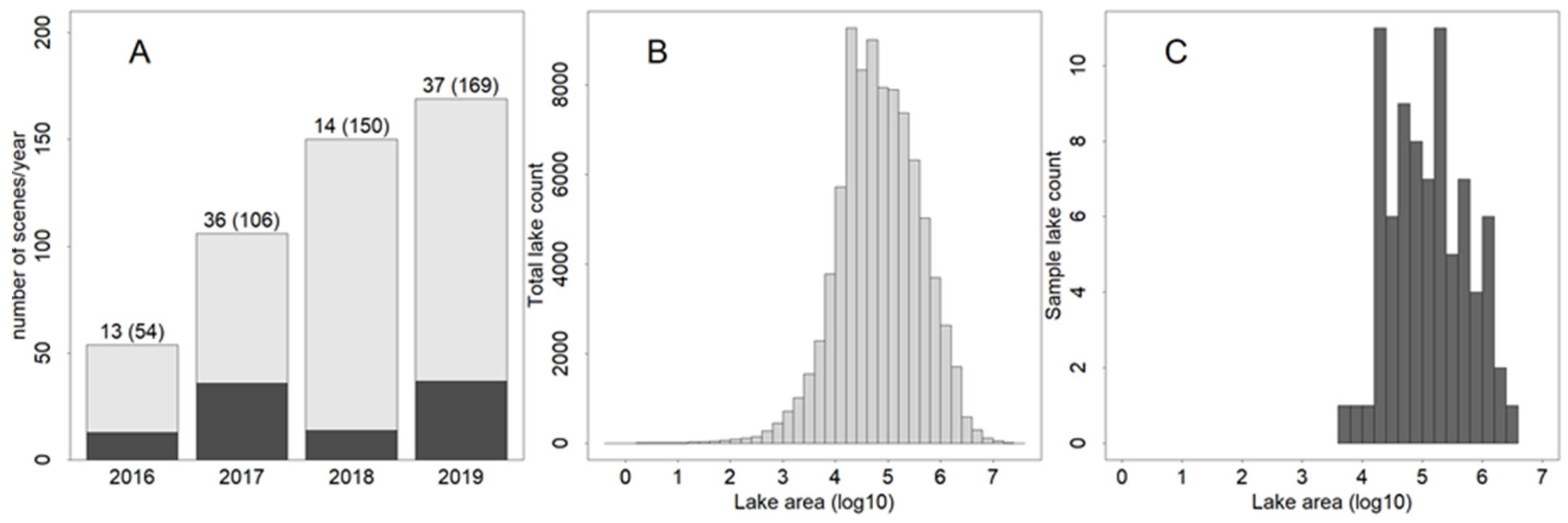
For the whole period, lakes appeared in 880 of the 1035 sinks. The majority of all lakes (93.73%) have an area below 1 km2 (Figure 4B). These lakes account for 48.63% of the total detected lake area between 2016 and 2019. The largest single lake detected has an area of 30.49 km2 and appeared on 29 July 2019. The mean/median SGL size is 274,540/64,212 m2, with a standard deviation of 775,750 m2. In total, the 10 S-2 granules cover an area of 82,427 km2, with the ablation mask covering 27,504 km2. The mean/median error is 2505/3870 m2 per lake, or 0.044/0.024 m2 per pixel (100 m2).
3.1. Interannual Differences in Total Lake Area
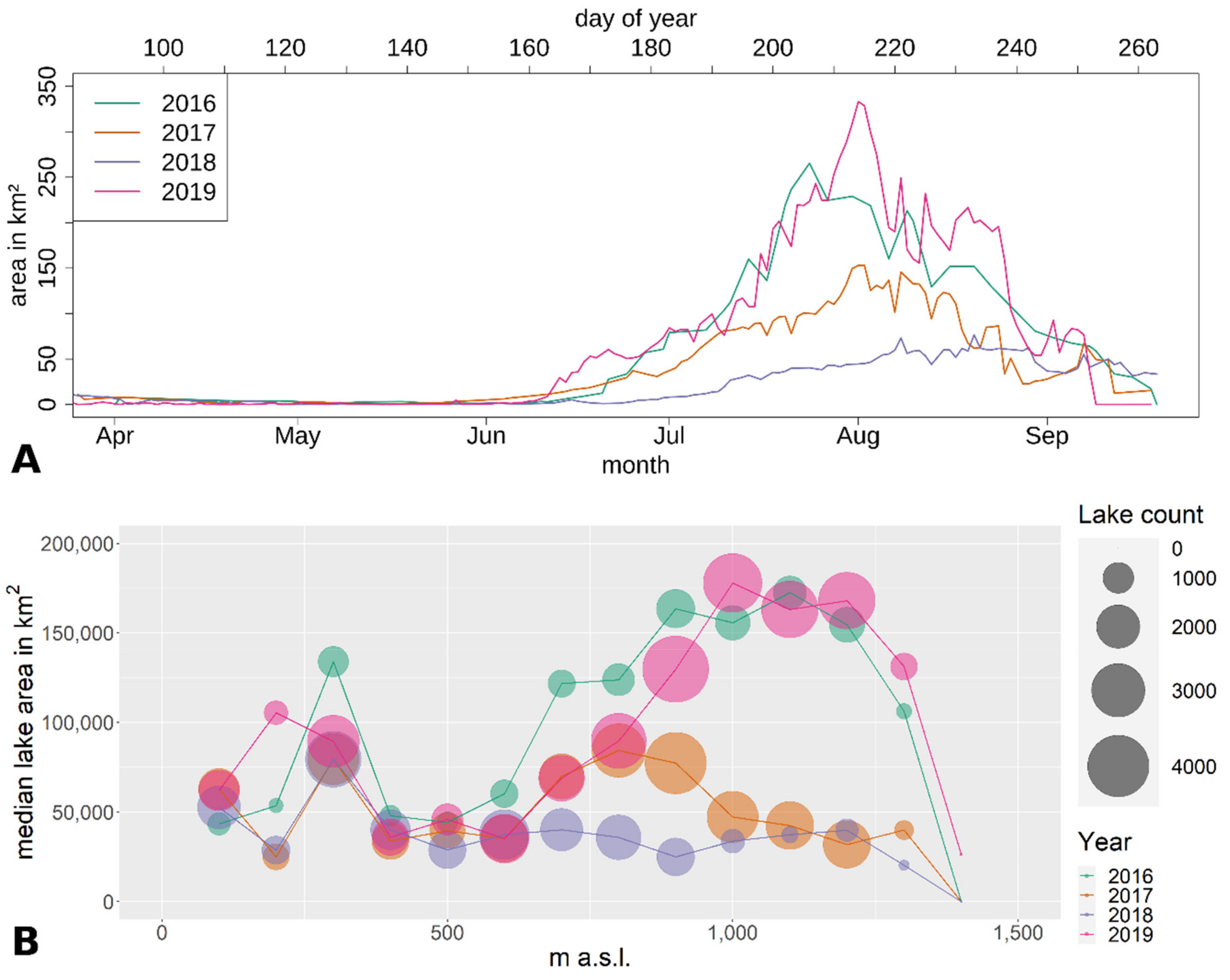
Figure 5A shows the cumulated lake area for each analyzed date between 2016 and 2019. Among the three years, 2019 has the highest daily SGL area (333.19 km2 on 2 August), four times larger than in 2018 (76.66 km2 on 21 August). The maximum occurred earliest in 2016 (24 July) and latest in 2018 (21 August). The maximum daily number of lakes is the largest in 2019 (553), followed by 2016 (477), 2017 (423) and 2018 (288).
The melt onset can be defined as the date when free water is continuously present in the snowpack [45]. After a few days of continuous melt days, SGL becomes visible through the melt of covering ice or the confluence of mobile water. GL appeared earliest in 2017 and disappeared latest in 2018, the latter being delayed by 25 and 14 days compared to 2017 and 2016, respectively (Table 3). Though 2018 thus has the latest appearance and simultaneously the lowest maximum total lake area, maximum lake extent and number generally do not seem correlated with the timing of the melt season.
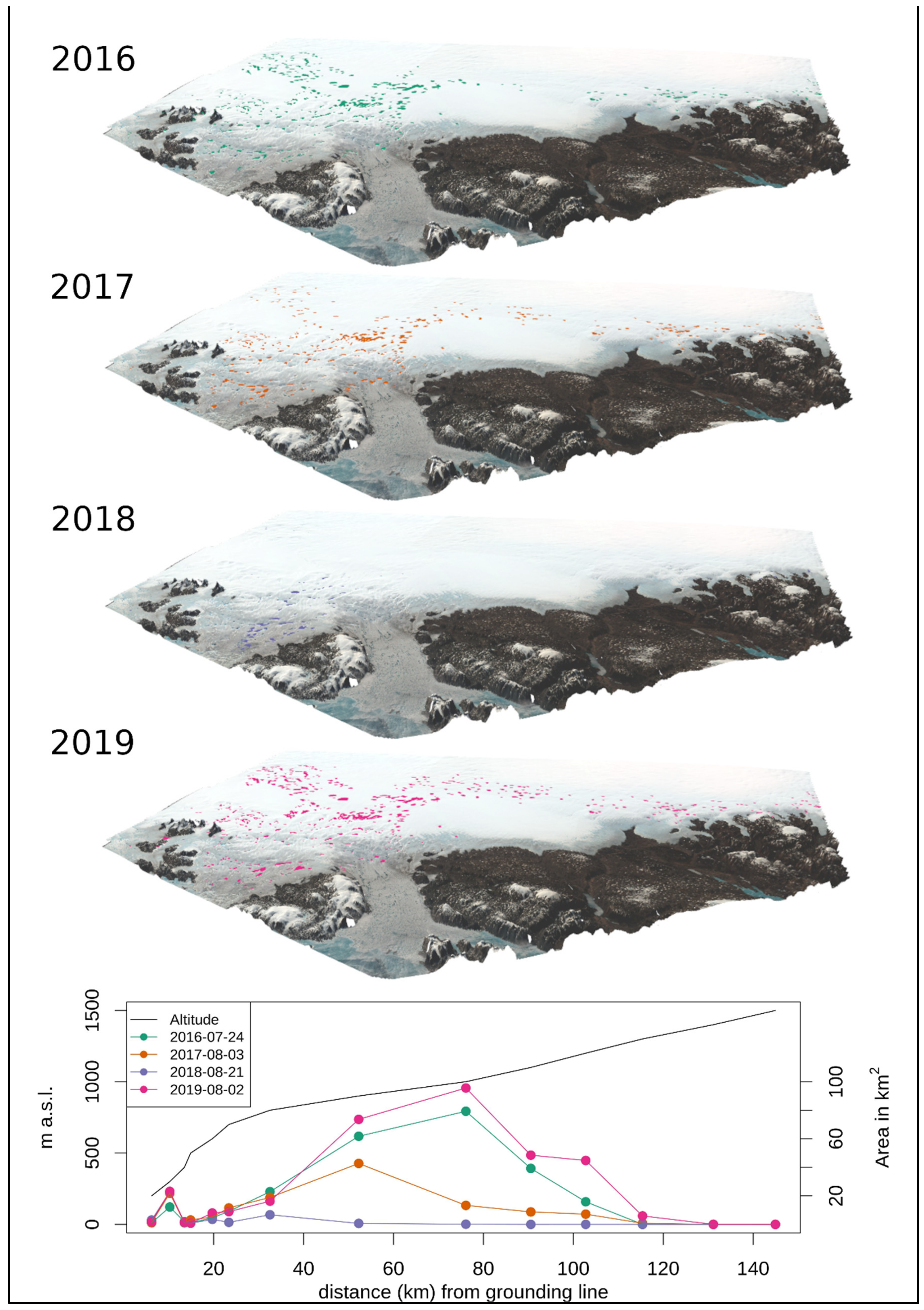
3.2. Lake Altitude and Spatial Patterns
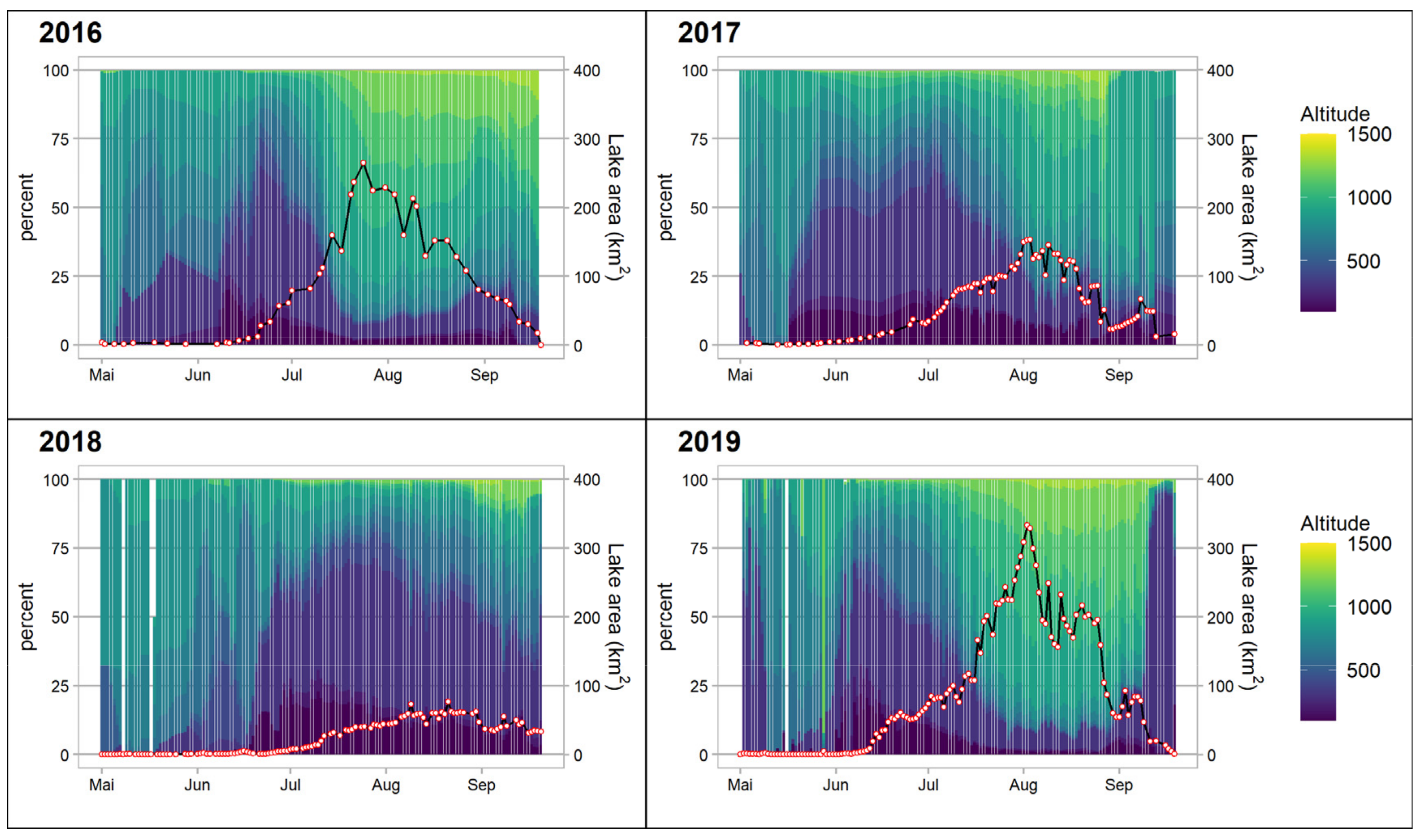
During 2016, 2017 and 2019, the highest number of lakes developed between 851 and 950 m a.s.l. (Figure 5B). For 2016 and 2019, this altitude also showed the largest SGL area extent of all elevation bins (Figure 6), whereas, for 2017, lakes between 751 and 850 m a.s.l. had the largest extent. This distribution coincides with the gentlest slopes of the glacier surface between 750 and 950 m a.s.l. (Figure 7). The transition phase from the majority of lake area being located below 750 m a.s.l. to above is short in 2016 and 2019, from 80% to 20% of the lake area appearing below 750 m a.s.l. within 20 days for both years. This period is accompanied by an area increase of 170 km2 in both years, cumulating into the maximum of 265.39 km2 in 2016 (Figure 6).
4. Discussion
4.1. Consistency with Previous Studies
4.1.1. Northeast Greenland
Two studies have previously focused on SGL detection in the northeast Greenland sector, though the study by Selmes and colleagues [32] also contains data from northeast Greenland.
The first study by Sundal and colleagues [13] using MODIS covers the period 2003 to 2007. They report maximum daily SGL areas between 81.1 (2006) and 149.6 (2003) km2, which is significantly less than our assessment (Table 2), though the lowest maxima are comparable (76.66 km2 in 2018). This can be explained by mainly three factors: (1) the resolution of MODIS is 250 m/pixel (Figure A3); thus, the minimum detectable SGL size is 62,500 km2, thus lakes smaller than 0.1 km2 were not included in the study. For our dataset, these lakes account for 58.78% of all lakes in number and 7% of the total SGL area. (2) The former study reports lakes up to 1200 m a.s.l., whereas we found lakes up to 1400 m. This corroborates the findings of Gledhill and Williamson [4], who report a maximum elevation gain of SGL of 418 m between 1985 and 2016 at a rate of 13.5 m/year. For the maximum of 2019, lakes at elevations between 1200 m and 1400 m sum up to 50.7 km2, accounting for 15% of the lake area for this day. For 2016, this difference is 15.9 km2/6%. (3) Sundal and colleagues report an area of interest between 78.21°N and 79.5°N covering 17,500 km2, whereas our dataset covers 78.21°N to 81°N. Lakes between 79.5°N and 81°N cover an area of 36.99 km2 for the maximum of 2019, accounting for 14.53% of this day’s SGL area. Nonetheless, it should be noted that our study probably underestimates the true lake area (Section 4.2) and that the difference may be even higher. Regarding timing, the results are generally in agreement: the maxima are reached between DOY 202 and 223 for the former study, and between DOY 206 and 233 in this study, with the dates being subject to data availability. The active melt season varies between DOY 160–180 (143–164) and DOY 258–278 (253–263) for the former study (this study).
The second and newer study by Schröder and colleagues [12] mainly employs polarimetric SAR (Sentinel-1), but also involves data from Sentinel-2 and covers the period 2017–2020. Their research area covers 76 to 80°N and −22 to −34°W, up to >2000 m a.s.l. As two datasets with different properties and results are involved, they need to be compared individually to the outcome of this study. In general, the SAR-based method results in significantly larger water areas (up to a factor of 3) than the S-2 based detection methods. We attribute this difference mainly to (a) the difference between the measured electromagnetic spectra and thus the measured properties of the ground, (b) the inability of multispectral sensors to penetrate ice and snow, and (c) the different definitions of SGL. The classification of the Sentinel-1 backscatter is mainly based on the total reflection of the microwaves away from the sensor and a resulting minimal backscatter due to the side-looking geometry of the SAR sensor. Additionally, microwaves from the C-band are able to penetrate snow, dependent on its water content and ice [46]. Potentially, these properties can be utilized to measure the total water content of the glacier surface, including liquid water covered by frozen surfaces. The latter is a major advantage over Sentinel-2 based classifications, where only visible water can be detected. On the other hand, the SAR detection is heavily influenced by liquid precipitation and the high water content in snow during the main melt season [12]. Consequently, it is probable that, during summer, SAR SGL detection overestimates lake areas, whereas multispectral methods underestimate the true lake area during the early and late melt season. Therefore, a direct comparison of the total lake area is challenging. For the Sentinel-2 dataset in the former study, the total lake area is generally smaller than within our study, except for the maximum extent of 2019. We attribute this mainly to the use of the NDWI with a threshold tested for west Greenland. Due to the difference in radiation between 70°N and 79°N, a tuning of the threshold to local conditions would probably have resulted in larger lake areas [47].
4.1.2. Comparison with Other Areas in Greenland
A wealth of studies focusing on SGLs were performed in the perimeter of Jakobshavn Glacier, West Greenland (Figure 1) using MODIS, Landsat, ASTER, or a combination of these sensors. Due to the large number which would require a distinct review article to compare, and the fact that most of the studies focus on determining lake depths and volumes, we concentrate on studies (a) of great spatial extent, e.g., the whole ice sheet, and (b) time-series studies, as these may deliver similar parameters such as melting season, annual maxima, etc.
Of the sheet-wide studies, Selmes and colleagues [32] found a mean/median lake area of 0.80/0.56 km2 (0.63 km2 for northeast Greenland), which is large compared to our results but may be influenced by the minimum resolution of MODIS, preventing a large number of small lakes from being detected (Section 3). Additionally, they report a maximum lake size of 16.8 km2 for the whole Greenland Ice Sheet (GrIS), and a mean total lake area of 268 ± 79 km2 for northeast Greenland between 2005 and 2009. We attribute the differences, especially in maximum lake size, to an upward migration of the ELA, especially in warm years, and consequently an increase of the ablation area in higher altitudes. This is in accordance with Liang and colleagues [48] as well as Gledhill and Williamson [4], who confirmed that SGL area in high altitudes could vary largely, and single lakes may even drive the dynamics of the whole SGL area for a region. As a contrast, we found lakes close to the grounding line to exhibit similar areas independent of the year, which is in accordance with previous time-series studies [22,48,49].
The peaks in the total lake area as reached in late July/early August, appear roughly two to four weeks later than at Petermann Glacier [19], as well as in West Greenland [23], though Fitzpatrick and colleagues report a spread of the date of maximum total lake volume between 5 June and 8 August for the period 2002 to 2012 [15].
4.2. Area Delineation Performance
4.2.1. Static Band Ratio
The similarity of the spectral information of topographic shadows and water in the blue and red band, compared to the near- and shortwave infrared, is a major disadvantage of the B/R ratio and requires correction in postprocessing. When processing time-series, the computation of the binary topographic shadow masks are required for each acquisition and each granule to be analyzed. For the S-2 NDWI, either band 8 (NIR, 10 m resolution) or band 12 (SWIR, 20 m resolution) needs to be resampled for each date. Consequently, from a computation time perspective, NDWI is better suited for short time-series, as processing shadow masks is time-consuming. Longer time-series, however, profit from the pre-computed shadow masks so that the B/R ratio outperforms NDWI at a certain point, which is subject to hardware resources and a number of scenes in question. For areas without considerable topographic shadows, NDWI and B/R ratio without correction can be expected to deliver similar results [47].
The majority of studies on SGLs use a band ratio with dynamic thresholding [29,32,50]. In theory, this approach is superior to static thresholding, as it is less vulnerable to low contrast, as, e.g., with low sun angles, or if half-transparent cirrus clouds are present. Thus, it may prevent outliers and is potentially applicable to larger areas [29]. Our decision for a static threshold was mainly driven by the computational effort, which is less for static band ratios and thus preferable for large datasets given limited resources. Leeson and colleagues [51] suggested the combination of three different methods for the best accuracy regarding lake size and number, which would have tripled the processing and analysis time. In addition, Williamson and colleagues found that B/R ratio static thresholding resulted in lower RMSE values than other SGL area algorithms if tuned to the study region [47]. Thus, we are confident that our approach is adequate given the high number of scenes, but if applied to other regions, the static threshold should be adapted or replaced by a dynamic threshold if simultaneous analyses of different areas are desired.
4.2.2. Cloud Correction
Step 1 of the cloud correction implements a time-dependent control that is based on the dynamic nature of weather over northeast Greenland, e.g., with respect to the position and strength of the jet stream and the NAO or the occurrence of katabatic winds or piteraqs [52,53]. Though it is reasonable to assume that a lake is not masked by the same cloud for several days, an obscuring for more than one scene is likely. The relatively long threshold of ±15 days, covering ±10 scenes on average, increases the chance of finding a cloud-free observation. This comes at the cost of the detection of rapid lake drainage and refilling, which may happen in less than seven days [48,54], and the dis- and reappearance of a lake within this period will be classified as clouded. As such, this classification step, as well as step 2, acts as a low-pass filter for individual lakes. In addition, it is not possible to detect partial cloud coverage of lakes using this procedure. The differentiation between partial cloud cover and partial drainage does necessarily involve data from either other bands or data sources.
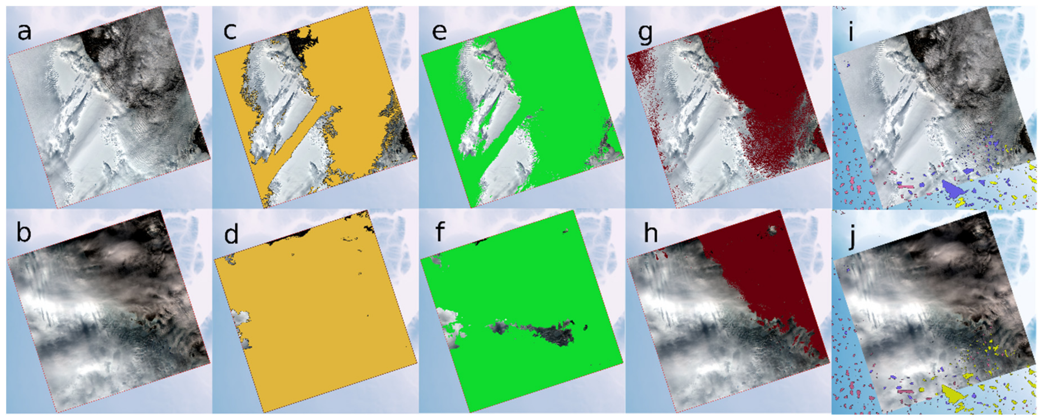
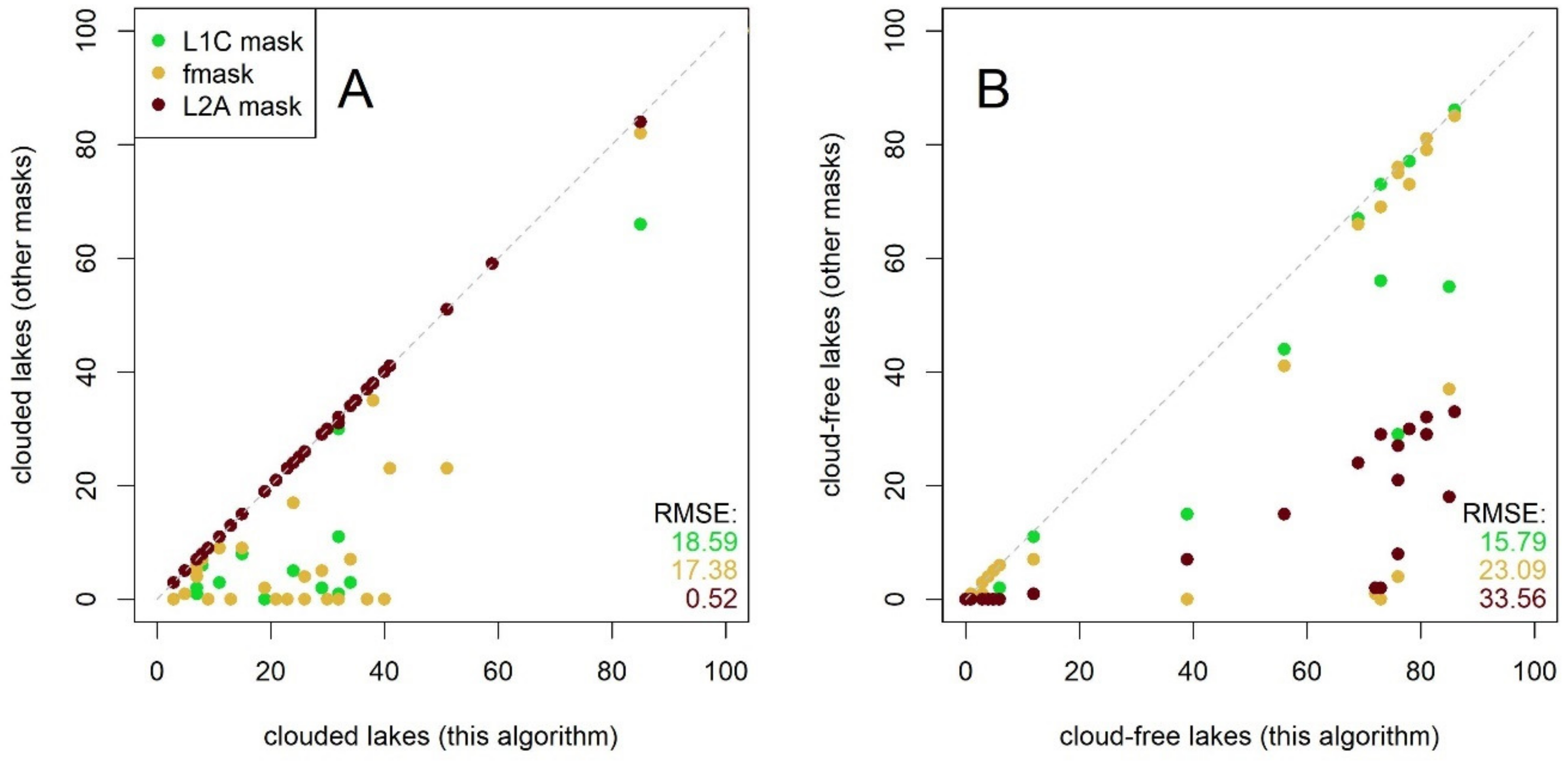
To quantify the performance of cloud detection algorithms is a challenging subject, as, aside from manually labeled datasets, no validation data exists. As manual classification is a time-consuming task that additionally requires training, result validation is typically done on a limited number of scenes, of which only a small percentage, if at all, covers snow- or ice-capped surfaces [55,56,57,58]. As a comparison of algorithm performance, or an error estimation for either the L1C-, Level-2A (L2A) cloud masks or fmask over ice are currently lacking, we compared the results of our cloud correction algorithms for 50 randomly chosen S2 scenes (granules 26XMP and 26XNP) to fmask and the L1C- and L2A classification masks (Figure 8). The different cloud masks have individual properties, e.g., fmask differentiates between several land cover types with clouds as one category, the L2A cloud mask grades clouds by thickness/type, and the L1C cloud mask is simply binary. To compare these different types, we generated binary cloud masks, in the case of fmask containing only the categories clouds and else, and in the case of the L2A mask, all values deviating from 0 were classified as clouds. For our cloud correction, we used the cloud classification matrix to classify the sinks as clouded or cloud-free, regardless of actual lake size.
Again, a classification of a cloud mask as even partially wrong is ambivalent, as, through thin clouds, lakes may be detectable. Thus, a potentially high percentage of detected lakes that are classified as cloud-covered is likely. To quantify the potential error adequately, we therefore also compared the lakes classified as cloudy by our procedure to their cloud cover by the other masks (Figure 9).
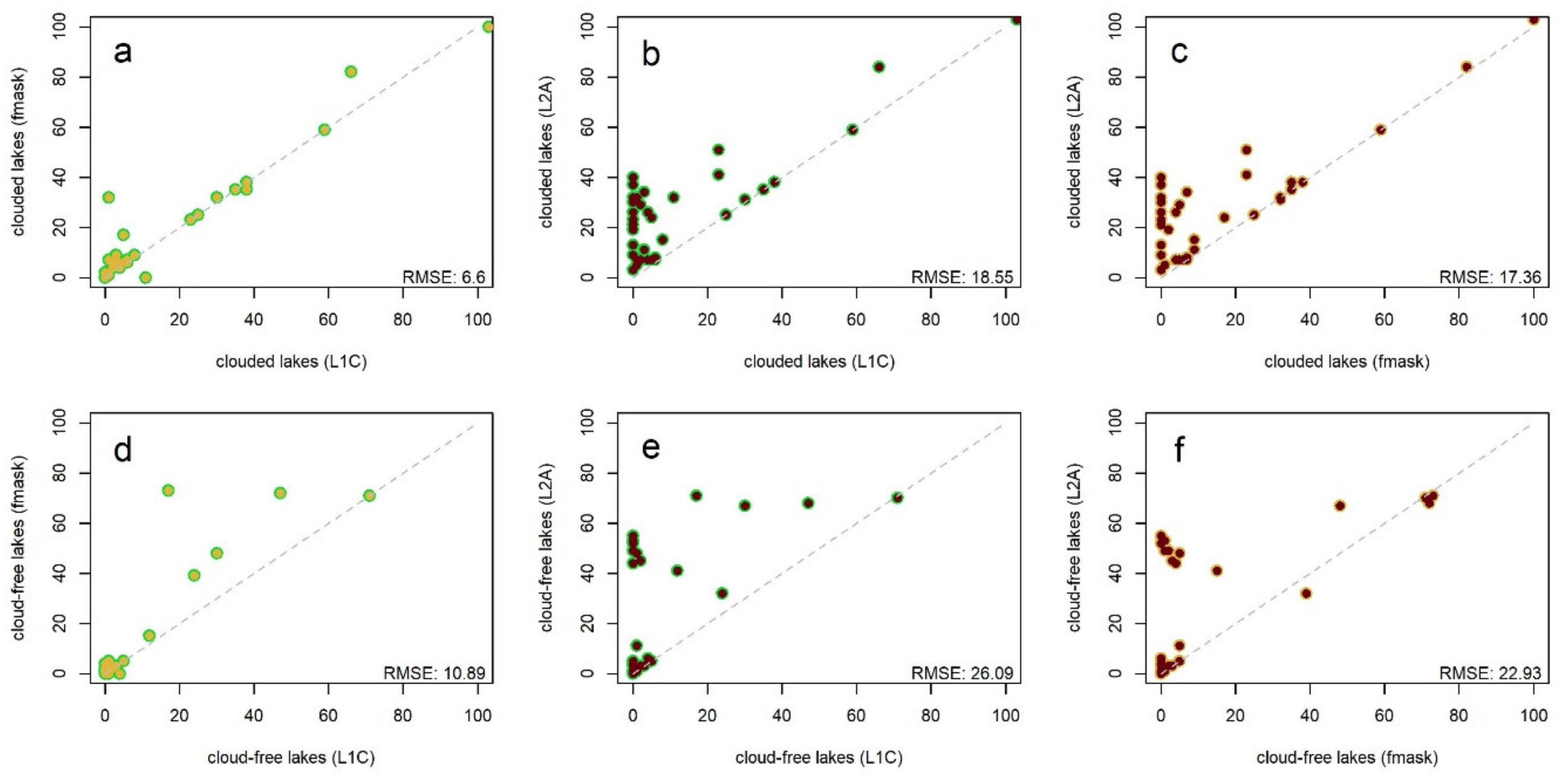
The standard Level 1C cloud mask performs best on average. The fit of fmask, especially for the cloud-free lakes, is strongly influenced by few heavy outliers (Figure 9B), whereas the L2A cloud mask obviously overestimates cloud cover. The latter is presumably skewed by our classification of light clouds as thick clouds. Comparing the fit of the three cloud masks among each other, the L1C mask and fmask generally exhibit the least differences (RMSE 10.89 for cloud-free lakes and 6.60 for clouded lakes, see Figure A4).
As these relations are relative to the cloud detection implemented in our processing chain, these values must be regarded with caution, as we cannot assume the cloud detection works perfectly and is probably still prone to errors, e.g., arising from partial cloud cover, cloud shadows, or drainage events. Thus, the need for a better performing cloud detection over ice and snow persists, and the results of this study would benefit substantially from new and more exact approaches in this field.
4.2.3. Lake Drainage Detection
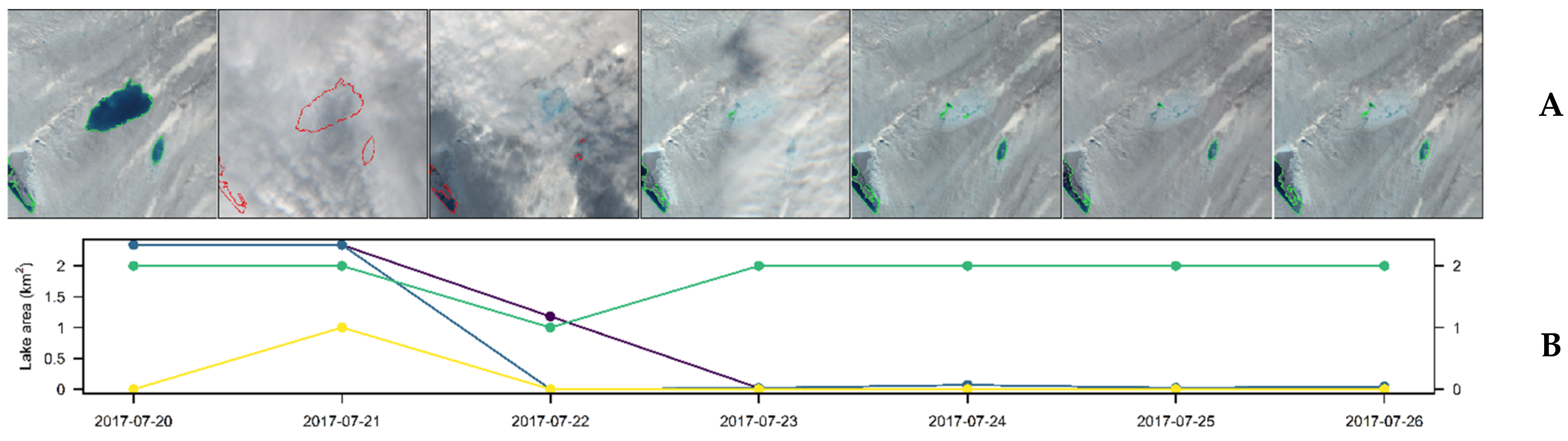
Rapid lake drainage events are one of the most interesting features of SGL, as these may lead to a (local) increase in ice velocity [6,59,60]. Our SGL time-series offers, through its high temporal and spatial resolution, the chance to detect rapid lake drainage events occurring in less than two days. We tested the potential of the improved temporal and spatial resolution on a known drainage event analyzed by Schröder and colleagues [12]. The lake (ID 577 in our dataset), located at N 78.87 W 21.73, has been found to drain completely between 20 July 2017 and 26 July 2017 (Figure 10).
Within the seven-day period, the lake size is reduced from 2.34 km2 to 0.04 km2, equal to 1.83% of the original lake area. Due to the daily resolution of our dataset within this period, the timing of the drainage event can be narrowed down to have occurred between 20 July and 23 July 2017, thus complying with the criteria for rapid drainage events by Morriss et al. [23], Fitzpatrick et al. [15] and Liang et al. [48]. A more exact determination of the event is hindered by thick cloud cover, a problem that has been discussed in detail by Cooley and Christoffersen [28]. According to the classification proposed in their study, a lake must drain 90% of its maximum area within 24 h (given daily observations with MODIS) to be classified as rapidly draining, while cloud-covered observations are excluded from this period. As stated in Section 4.2.2, our two-step cloud detection prevents, in probably most cases, the classification of an area reduction as rapid lake drainage due to the interpolation interval of maximum15 days. This is perfectly illustrated by the example in Figure 10, as the lake loses more than 90% of its area within 48 h; without consultation of the cloud masks, this would, following Cooley and Christoffersen [28], not be classified as rapidly draining. As 21 July is flagged as cloud-covered by cloud mask #1 and 22 July by cloud mask #2 (Figure 10), the drainage event should be classified as rapid. This corroborates the findings that there is an observation bias in rapid drainage event analyses based on multispectral satellite data due to cloud cover, hindering rapid drainage events from being defined as such. We strongly agree that cloud masks, if available, should be considered in the definition of the speed of lake drainage events.
4.3. Error Discussion
The calculated root means squared error (RMSE) between both sample datasets sums up to 189,377.2 m2 (Figure 11A). This compares well to the root mean square deviation (RSMD) of 0.22 km2 given by Sundal and colleagues [13], who compared a sample of 53 lakes obtained from MODIS and ASTER imagery. In contrast to the RMSD of 0.007 km2 given by Williamson and colleagues [9] using S-2 and Landsat 8, the RMSE is large; this can be reasoned by several points: (i) the cloud correction implemented is still inferior to manual checks, (ii) manually delineated lakes as ground truth sample introduce a larger error compared to Landsat-derived lakes, where the same methodology was applied and (iii) large errors in our sample dataset that mainly stem from low contrasts, with static thresholding probably producing less exact results in these cases (Figure 11C).
Setting a threshold to delineate ice from water is potentially risky, as the transition from solid to fluid is not separated by a sharp border, but continuously, with intermediate states such as slush; also, if the water is covered by an ice layer, the depth of the underlying lake influences the reflectance, both of which have a continuous measure. As to this day, the only way to minimize classification errors is an expert-driven manual mapping; every automated procedure is a compromise between quantity and quality. Due to increasing quality, detail and sources of satellite data, this conflict could potentially be minimized through the increasing use of deep learning and/or artificial intelligence, both of which are able to include the time domain in the analysis, and thus the evolution of the glacier surface. Our approach to reducing the possible error through empirical identification of the most precise threshold and the integration of the time domain in postprocessing nevertheless aims at the best possible and most realistic results, though an exact error cannot be quantified.
5. Conclusions
Multiple studies mapping SGLs in Greenland have used MODIS, albeit its low spatial resolution, or Landsat, which suffers from long repeat cycles, preventing short-term glaciological or climate-induced processes from being detected. For all multispectral sensors, cloud cover, especially over snow and ice, is an obstacle that is hard to overcome using band combinations alone, thus hindering fully automated image processing and requiring manual inspection of the data.
In this study, we explore the potential of S-2 to detect SGL in a fully automated way. S-2 combines the merits of both MODIS (high temporal resolution) and Landsat (high spatial resolution), especially in high latitudes. For the melt seasons 2016 to 2019, we detected 880 lakes with a minimum size of 0.015 km2 and an average temporal resolution of 1.5 days. The main improvements on the few previous studies employing S-2 for this purpose are (a) the consideration of topographic shadows, limiting the error induced by the spectral similarity of shadows and water on ice, and (b) the implementation of a two-step cloud filter that does not require manual inspection, and takes spatiotemporal characteristics of clouds and lakes into account. The high temporal density of the dataset enables the detection of rapid lake drainages as well as the analysis of the glacier surface’s changes due to local weather phenomena, potentials which have only been initially tapped in this study and demand for in-depth exploration of the data. As with all studies employing multispectral data, clouds still introduce a potential source of error; thus, the accuracy of the algorithms will benefit from any future progress in cloud detection using S-2 [61].
The whole processing chain was developed using free and open-source software alone. It enabled us to detect and track 880 SGLs over four years, allowing insights into spatial and temporal properties of surface melt of the NEGIS. The processing chain is designed to be converted into a continuously running version with only minor changes, so near real-time changes can be detected. Given the availability of cloud computing and the continuous increase of storage and computation capabilities, the algorithms are also scalable to investigate SGLs over larger areas or even the whole Greenland Ice Sheet.
Author Contributions
Conceptualization, P.H. and M.B.; methodology, P.H., N.N. and N.R.; software, P.H., N.N. and N.R.; validation, P.H.; formal analysis, P.H.; investigation, P.H.; resources, P.H. an N.N.; data curation, P.H.; writing—original draft preparation, P.H. and N.N.; writing—review and editing, N.R., M.B. and A.H.; visualization, P.H.; supervision, M.B. and A.H.; project administration, M.B. and A.H.; funding acquisition, M.B. and A.H. All authors have read and agreed to the published version of the manuscript.
Funding
This research was funded by the German Federal Ministry of Education and Research (BMBF) through the joint project GROCE—Greenland Ice Sheet Ocean Interaction, grant number 03F0778F.
Institutional Review Board Statement
Not applicable.
Informed Consent Statement
Not applicable.
Data Availability Statement
Lake outline polygons for 79 N as well as cloud masks are currently available on request and will be uploaded to Pangaea Data Center after manuscript publication.
Acknowledgments
We are grateful to the European Space Agency (ESA) for providing the Sentinel-1 and Sentinel-2 data and Brice Noël for providing the RACMO 2.3 data.
Conflicts of Interest
The authors declare no conflict of interest. The funders had no role in the design of the study; in the collection, analyses, or interpretation of data; in the writing of the manuscript, or in the decision to publish the results.
Appendix A
Figure A1.
Average solar elevation for all granules at the time of sensing by S-2 for each day coverage of the whole AOI could be retrieved. Black line is the mean smoothed by local regression; all circle centers in the gray area fall within one standard deviation from the mean. Minimum solar elevation is 79.6° from nadir on 19 September 2017; maximum is 55.7° from nadir on 22 June 2018.

Figure A2.
Algorithm for calculating topographic shadows for the whole area of interest (AOI) per day, executed for each date with full coverage. Rectangles are input/output data; diamonds are processes.
Figure A2.
Algorithm for calculating topographic shadows for the whole area of interest (AOI) per day, executed for each date with full coverage. Rectangles are input/output data; diamonds are processes.

Figure A3.
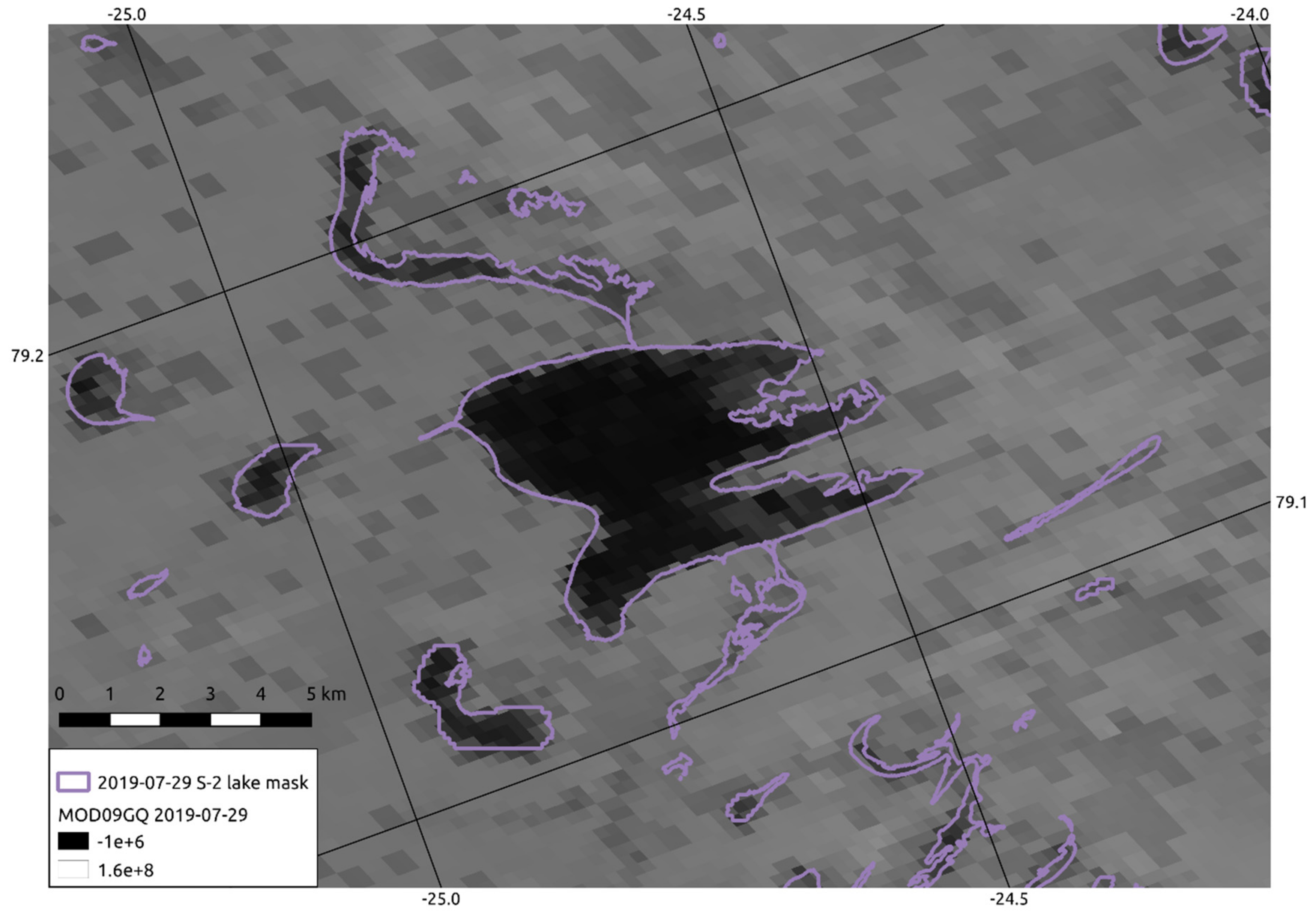
Influence of pixel size on lake detection: contours of the largest detected lake using Sentinel-2 on 29 July 2019, against MODIS band 1 reflectance of the same day (MOD09GQ, 250 m resolution).
Figure A3.
Influence of pixel size on lake detection: contours of the largest detected lake using Sentinel-2 on 29 July 2019, against MODIS band 1 reflectance of the same day (MOD09GQ, 250 m resolution).

Figure A4.
Relations for the clouded (a–c) and cloud-free (d–f) test data for the L1C-, fmask- and L2A cloud masks, with the respective RMSE. Color-code as displayed in Figure 9.
Figure A4.
Relations for the clouded (a–c) and cloud-free (d–f) test data for the L1C-, fmask- and L2A cloud masks, with the respective RMSE. Color-code as displayed in Figure 9.

References
- Bevis, M.; Harig, C.; Khan, S.A.; Brown, A.; Simons, F.J.; Willis, M.; Fettweis, X.; van den Broeke, M.R.; Madsen, F.B.; Kendrick, E.; et al. Accelerating Changes in Ice Mass within Greenland, and the Ice Sheet’s Sensitivity to Atmospheric Forcing. Proc. Natl. Acad. Sci. USA 2019, 116, 1934–1939. [Google Scholar] [CrossRef] [PubMed] [Green Version]
- Moon, T.; Joughin, I.; Smith, B.; Howat, I. 21st-Century Evolution of Greenland Outlet Glacier Velocities. Science 2012, 336, 576–578. [Google Scholar] [CrossRef] [PubMed] [Green Version]
- Rignot, E.; Kanagaratnam, P. Changes in the Velocity Structure of the Greenland Ice Sheet. Science 2006, 311, 986–990. [Google Scholar] [CrossRef] [PubMed] [Green Version]
- Gledhill, L.A.; Williamson, A.G. Inland Advance of Supraglacial Lakes in North-West Greenland under Recent Climatic Warming. Ann. Glaciol. 2017. [Google Scholar] [CrossRef] [Green Version]
- Miles, K.E.; Willis, I.C.; Benedek, C.L.; Williamson, A.G.; Tedesco, M. Toward Monitoring Surface and Subsurface Lakes on the Greenland Ice Sheet Using Sentinel-1 SAR and Landsat-8 OLI Imagery. Front. Earth Sci. 2017, 5. [Google Scholar] [CrossRef] [Green Version]
- Tedesco, M.; Willis, I.C.; Hoffman, M.J.; Banwell, A.F.; Alexander, P.; Arnold, N.S. Ice Dynamic Response to Two Modes of Surface Lake Drainage on the Greenland Ice Sheet. Environ. Res. Lett. 2013, 8, 034007. [Google Scholar] [CrossRef]
- Vijay, S.; Khan, S.A.; Kusk, A.; Solgaard, A.M.; Moon, T.; Bjørk, A.A. Resolving Seasonal Ice Velocity of 45 Greenlandic Glaciers With Very High Temporal Details. Geophys. Res. Lett. 2019, 46, 1485–1495. [Google Scholar] [CrossRef] [Green Version]
- Pitcher, L.H.; Smith, L.C. Supraglacial Streams and Rivers. Annu. Rev. Earth Planet. Sci. 2019, 47, 421–452. [Google Scholar] [CrossRef] [Green Version]
- Williamson, A.G.; Banwell, A.F.; Willis, I.C.; Arnold, N.S. Dual-Satellite (Sentinel-2 and Landsat 8) Remote Sensing of Supraglacial Lakes in Greenland. Cryosphere 2018, 12, 3045–3065. [Google Scholar] [CrossRef] [Green Version]
- Yang, K.; Smith, L.C.; Sole, A.; Livingstone, S.J.; Cheng, X.; Chen, Z.; Li, M. Supraglacial Rivers on the Northwest Greenland Ice Sheet, Devon Ice Cap, and Barnes Ice Cap Mapped Using Sentinel-2 Imagery. Int. J. Appl. Earth Obs. Geoinf. 2019, 78, 1–13. [Google Scholar] [CrossRef] [Green Version]
- Box, J.E.; Ski, K. Remote Sounding of Greenland Supraglacial Melt Lakes: Implications for Subglacial Hydraulics. J. Glaciol. 2007, 53, 257–265. [Google Scholar] [CrossRef] [Green Version]
- Schröder, L.; Neckel, N.; Zindler, R.; Humbert, A. Perennial Supraglacial Lakes in Northeast Greenland Observed by Polarimetric SAR. Remote Sens. 2020, 12, 2798. [Google Scholar] [CrossRef]
- Sundal, A.V.; Shepherd, A.; Nienow, P.; Hanna, E.; Palmer, S.; Huybrechts, P. Evolution of Supra-Glacial Lakes across the Greenland Ice Sheet. Remote Sens. Environ. 2009, 113, 2164–2171. [Google Scholar] [CrossRef]
- Ignéczi, Á.; Sole, A.J.; Livingstone, S.J.; Leeson, A.A.; Fettweis, X.; Selmes, N.; Gourmelen, N.; Briggs, K. Northeast Sector of the Greenland Ice Sheet to Undergo the Greatest Inland Expansion of Supraglacial Lakes during the 21st Century: Expansion of Surface Lakes on the GrIS. Geophys. Res. Lett. 2016, 43, 9729–9738. [Google Scholar] [CrossRef] [Green Version]
- Fitzpatrick, A.A.W.; Hubbard, A.L.; Box, J.E.; Quincey, D.J.; van As, D.; Mikkelsen, A.P.B.; Doyle, S.H.; Dow, C.F.; Hasholt, B.; Jones, G.A. A Decade (2002–2012) of Supraglacial Lake Volume Estimates across Russell Glacier, West Greenland. Cryosphere 2014, 8, 107–121. [Google Scholar] [CrossRef] [Green Version]
- Georgiou, S.; Shepherd, A.; McMillan, M.; Nienow, P. Seasonal Evolution of Supraglacial Lake Volume from ASTER Imagery. Ann. Glaciol. 2009, 50, 95–100. [Google Scholar] [CrossRef] [Green Version]
- Hoffman, M.J.; Perego, M.; Andrews, L.C.; Price, S.F.; Neumann, T.A.; Johnson, J.V.; Catania, G.; Lüthi, M.P. Widespread Moulin Formation During Supraglacial Lake Drainages in Greenland. Geophys. Res. Lett. 2018, 45, 778–788. [Google Scholar] [CrossRef] [Green Version]
- Johansson, A.M.; Brown, I.A. Observations of Supra-Glacial Lakes in West Greenland Using Winter Wide Swath Synthetic Aperture Radar. Remote Sens. Lett. 2012, 3, 531–539. [Google Scholar] [CrossRef]
- Lampkin, D.J.; VanderBerg, J. A Preliminary Investigation of the Influence of Basal and Surface Topography on Supraglacial Lake Distribution near Jakobshavn Isbrae, Western Greenland. Hydrol. Process. 2011, 25, 3347–3355. [Google Scholar] [CrossRef]
- Legleiter, C.J.; Tedesco, M.; Smith, L.C.; Behar, A.E.; Overstreet, B.T. Mapping the Bathymetry of Supraglacial Lakes and Streams on the Greenland Ice Sheet Using Field Measurements and High-Resolution Satellite Images. Cryosphere 2014, 8, 215–228. [Google Scholar] [CrossRef] [Green Version]
- Liang, S. Narrowband to Broadband Conversions of Land Surface Albedo I. Remote Sens. Environ. 2001, 76, 213–238. [Google Scholar] [CrossRef]
- Macdonald, G.J.; Banwell, A.F.; MacAyeal, D.R. Seasonal Evolution of Supraglacial Lakes on a Floating Ice Tongue, Petermann Glacier, Greenland. Ann. Glaciol. 2018, 59, 56–65. [Google Scholar] [CrossRef] [Green Version]
- Morriss, B.F.; Hawley, R.L.; Chipman, J.W.; Andrews, L.C.; Catania, G.A.; Hoffman, M.J.; Lüthi, M.P.; Neumann, T.A. A Ten-Year Record of Supraglacial Lake Evolution and Rapid Drainage in West Greenland Using an Automated Processing Algorithm for Multispectral Imagery. Cryosphere 2013, 7, 1869–1877. [Google Scholar] [CrossRef] [Green Version]
- Pope, A.; Scambos, T.A.; Moussavi, M.; Tedesco, M.; Willis, M.; Shean, D.; Grigsby, S. Estimating Supraglacial Lake Depth in West Greenland Using Landsat 8 and Comparison with Other Multispectral Methods. Cryosphere 2016, 10, 15–27. [Google Scholar] [CrossRef] [Green Version]
- Smith, L.C.; Chu, V.W.; Yang, K.; Gleason, C.J.; Pitcher, L.H.; Rennermalm, A.K.; Legleiter, C.J.; Behar, A.E.; Overstreet, B.T.; Moustafa, S.E.; et al. Efficient Meltwater Drainage through Supraglacial Streams and Rivers on the Southwest Greenland Ice Sheet. Proc. Natl. Acad. Sci. USA 2015, 112, 1001–1006. [Google Scholar] [CrossRef] [PubMed] [Green Version]
- Sneed, W.A.; Hamilton, G.S. Evolution of Melt Pond Volume on the Surface of the Greenland Ice Sheet. Geophys. Res. Lett. 2007, 34, L03501. [Google Scholar] [CrossRef] [Green Version]
- Tedesco, M.; Steiner, N. In-Situ Multispectral and Bathymetric Measurements over a Supraglacial Lake in Western Greenland Using a Remotely Controlled Watercraft. Cryosphere 2011, 5, 445–452. [Google Scholar] [CrossRef] [Green Version]
- Cooley, S.W.; Christoffersen, P. Observation Bias Correction Reveals More Rapidly Draining Lakes on the Greenland Ice Sheet: Bias in Rapid Lake Drainage Detections. J. Geophys. Res. Earth Surf. 2017, 122, 1867–1881. [Google Scholar] [CrossRef]
- Selmes, N.; Murray, T.; James, T.D. Characterizing Supraglacial Lake Drainage and Freezing on the Greenland Ice Sheet. Cryosphere Discuss. 2013, 2013, 475–505. [Google Scholar] [CrossRef]
- Howat, I.M.; Negrete, A.; Smith, B.E. The Greenland Ice Mapping Project (GIMP) Land Classification and Surface Elevation Data Sets. Cryosphere 2014, 8, 1509–1518. [Google Scholar] [CrossRef] [Green Version]
- Mouginot, J.; Rignot, E.; Scheuchl, B.; Fenty, I.; Khazendar, A.; Morlighem, M.; Buzzi, A.; Paden, J. Fast Retreat of Zachariæ Isstrøm, Northeast Greenland. Science 2015, 350, 1357–1361. [Google Scholar] [CrossRef] [PubMed] [Green Version]
- Selmes, N.; Murray, T.; James, T.D. Fast Draining Lakes on the Greenland Ice Sheet. Geophys. Res. Lett. 2011, 38. [Google Scholar] [CrossRef]
- Shugar, D.H.; Burr, A.; Haritashya, U.K.; Kargel, J.S.; Watson, C.S.; Kennedy, M.C.; Bevington, A.R.; Betts, R.A.; Harrison, S.; Strattman, K. Rapid Worldwide Growth of Glacial Lakes since 1990. Nat. Clim. Chang. 2020. [Google Scholar] [CrossRef]
- Neckel, N.; Zeisig, O.; Steinhage, D.; Helm, V.; Humbert, A. Seasonal Observations at 79°N Glacier (Greenland) From Remote Sensing and in Situ Measurements. Front. Earth Sci. 2020, 8. [Google Scholar] [CrossRef]
- Noël, B.; van de Berg, W.J.; van Meijgaard, E.; Kuipers Munneke, P.; van de Wal, R.S.W.; van den Broeke, M.R. Evaluation of the Updated Regional Climate Model RACMO2.3: Summer Snowfall Impact on the Greenland Ice Sheet. Cryosphere 2015, 9, 1831–1844. [Google Scholar] [CrossRef] [Green Version]
- Racoviteanu, A.E.; Paul, F.; Raup, B.; Khalsa, S.J.S.; Armstrong, R. Challenges and Recommendations in Mapping of Glacier Parameters from Space: Results of the 2008 Global Land Ice Measurements from Space (GLIMS) Workshop, Boulder, Colorado, USA. Ann. Glaciol. 2009, 50, 53–69. [Google Scholar] [CrossRef] [Green Version]
- Corripio, J.G. Vectorial Algebra Algorithms for Calculating Terrain Parameters from DEMs and Solar Radiation Modelling in Mountainous Terrain. Int. J. Geogr. Inf. Sci. 2003, 17, 1–23. [Google Scholar] [CrossRef]
- GDAL Development Team. GDAL—Geospatial Data Abstraction Library; Version 2.2.2; Open Source Geospatial Foundation: Beaverton, OR, USA, 2018. [Google Scholar]
- Gudmundsson, G.H. Transmission of Basal Variability to a Glacier Surface: TRANSMISSION OF BASAL VARIABILITY TO A GLACIER SURFACE. J. Geophys. Res. Solid Earth 2003, 108. [Google Scholar] [CrossRef]
- Porter, C.; Morin, P.; Howat, I.; Noh, M.-J.; Bates, B.; Peterman, K.; Keesey, S.; Schlenk, M.; Gardiner, J.; Tomko, K.; et al. Arc-ticDEM. Harvard Dataverse, V1. 2018. Available online: https://dataverse.harvard.edu/dataset.xhtml?persistentId=doi:10.7910/DVN/OHHUKH (accessed on 6 December 2020).
- Lindsay, J.B. Whitebox GAT: A Case Study in Geomorphometric Analysis. Comput. Geosci. 2016, 95, 75–84. [Google Scholar] [CrossRef]
- Zhu, Z.; Wang, S.; Woodcock, C.E. Improvement and Expansion of the Fmask Algorithm: Cloud, Cloud Shadow, and Snow Detection for Landsats 4–7, 8, and Sentinel 2 Images. Remote Sens. Environ. 2015, 159, 269–277. [Google Scholar] [CrossRef]
- Hagolle, O.; Huc, M.; Desjardins, C.; Auer, S.; Richter, R. MAJA Algorithm Theoretical Basis Document. 2017. Available online: https://www.theia-land.fr/wp-content-theia/uploads/sites/2/2018/12/atbd_maja_071217.pdf (accessed on 6 December 2020).
- Paul, F.; Bolch, T.; Briggs, K.; Kääb, A.; McMillan, M.; McNabb, R.; Nagler, T.; Nuth, C.; Rastner, P.; Strozzi, T.; et al. Error Sources and Guidelines for Quality Assessment of Glacier Area, Elevation Change, and Velocity Products Derived from Satellite Data in the Glaciers_cci Project. Remote Sens. Environ. 2017, 203, 256–275. [Google Scholar] [CrossRef] [Green Version]
- Markus, T.; Stroeve, J.C.; Miller, J. Recent Changes in Arctic Sea Ice Melt Onset, Freezeup, and Melt Season Length. J. Geophys. Res. 2009, 114, C12024. [Google Scholar] [CrossRef]
- Nagler, T.; Rott, H.; Ripper, E.; Bippus, G.; Hetzenecker, M. Advancements for Snowmelt Monitoring by Means of Sentinel-1 SAR. Remote Sens. 2016, 8, 348. [Google Scholar] [CrossRef] [Green Version]
- Williamson, A.G.; Arnold, N.S.; Banwell, A.F.; Willis, I.C. A Fully Automated Supraglacial Lake Area and Volume Tracking (“FAST”) Algorithm: Development and Application Using MODIS Imagery of West Greenland. Remote Sens. Environ. 2017, 196, 113–133. [Google Scholar] [CrossRef]
- Liang, Y.-L.; Colgan, W.; Lv, Q.; Steffen, K.; Abdalati, W.; Stroeve, J.; Gallaher, D.; Bayou, N. A Decadal Investigation of Supraglacial Lakes in West Greenland Using a Fully Automatic Detection and Tracking Algorithm. Remote Sens. Environ. 2012, 123, 127–138. [Google Scholar] [CrossRef] [Green Version]
- Leeson, A.A.; Shepherd, A.; Briggs, K.; Howat, I.; Fettweis, X.; Morlighem, M.; Rignot, E. Supraglacial Lakes on the Greenland Ice Sheet Advance Inland under Warming Climate. Nat. Clim Chang. 2015, 5, 51–55. [Google Scholar] [CrossRef] [Green Version]
- Everett, A.; Murray, T.; Selmes, N.; Rutt, I.C.; Luckman, A.; James, T.D.; Clason, C.; O’Leary, M.; Karunarathna, H.; Moloney, V.; et al. Annual Down-Glacier Drainage of Lakes and Water-Filled Crevasses at Helheim Glacier, Southeast Greenland: DOWN-GLACIER SURFACE WATER DRAINAGE. J. Geophys. Res. Earth Surf. 2016, 121, 1819–1833. [Google Scholar] [CrossRef] [Green Version]
- Leeson, A.A.; Shepherd, A.; Sundal, A.V.; Malin Johansson, A.; Selmes, N.; Briggs, K.; Hogg, A.E.; Fettweis, X. A Comparison of Supraglacial Lake Observations Derived from MODIS Imagery at the Western Margin of the Greenland Ice Sheet. J. Glaciol. 2013, 59, 1179–1188. [Google Scholar] [CrossRef] [Green Version]
- Van As, D.; Fausto, R.S.; Steffen, K. Katabatic Winds and Piteraq Storms: Observations from the Greenland Ice Sheet. Geus Bull. 1969, 33, 83–86. [Google Scholar] [CrossRef] [Green Version]
- Turton, J.V.; Mölg, T.; Van As, D. Atmospheric Processes and Climatological Characteristics of the 79N Glacier (Northeast Greenland). Mon. Weather Rev. 2019, 147, 1375–1394. [Google Scholar] [CrossRef]
- Williamson, A.G.; Willis, I.C.; Arnold, N.S.; Banwell, A.F. Controls on Rapid Supraglacial Lake Drainage in West Greenland: An Exploratory Data Analysis Approach. J. Glaciol. 2018, 64, 208–226. [Google Scholar] [CrossRef] [Green Version]
- Doxani, G.; Vermote, E.; Roger, J.-C.; Gascon, F.; Adriaensen, S.; Frantz, D.; Hagolle, O.; Hollstein, A.; Kirches, G.; Li, F.; et al. Atmospheric Correction Inter-Comparison Exercise. Remote Sens. 2018, 10, 352. [Google Scholar] [CrossRef] [PubMed] [Green Version]
- Coluzzi, R.; Imbrenda, V.; Lanfredi, M.; Simoniello, T. A First Assessment of the Sentinel-2 Level 1-C Cloud Mask Product to Support Informed Surface Analyses. Remote Sens. Environ. 2018, 217, 426–443. [Google Scholar] [CrossRef]
- Baetens, L.; Desjardins, C.; Hagolle, O. Validation of Copernicus Sentinel-2 Cloud Masks Obtained from MAJA, Sen2Cor, and FMask Processors Using Reference Cloud Masks Generated with a Supervised Active Learning Procedure. Remote Sens. 2019, 11, 433. [Google Scholar] [CrossRef] [Green Version]
- Sanchez, A.H.; Picoli, M.C.A.; Camara, G.; Andrade, P.R.; Chaves, M.E.D.; Lechler, S.; Soares, A.R.; Marujo, R.F.B.; Simões, R.E.O.; Ferreira, K.R.; et al. Comparison of Cloud Cover Detection Algorithms on Sentinel–2 Images of the Amazon Tropical Forest. Remote Sens. 2020, 12, 1284. [Google Scholar] [CrossRef] [Green Version]
- Das, S.B.; Joughin, I.; Behn, M.D.; Howat, I.M.; King, M.A.; Lizarralde, D.; Bhatia, M.P. Fracture Propagation to the Base of the Greenland Ice Sheet During Supraglacial Lake Drainage. Science 2008, 320, 778–781. [Google Scholar] [CrossRef] [Green Version]
- Zwally, H.J. Surface Melt-Induced Acceleration of Greenland Ice-Sheet Flow. Science 2002, 297, 218–222. [Google Scholar] [CrossRef]
- Shendryk, Y.; Rist, Y.; Ticehurst, C.; Thorburn, P. Deep Learning for Multi-Modal Classification of Cloud, Shadow and Land Cover Scenes in PlanetScope and Sentinel-2 Imagery. ISPRS J. Photogramm. Remote Sens. 2019, 157, 124–136. [Google Scholar] [CrossRef]
Figure 1.
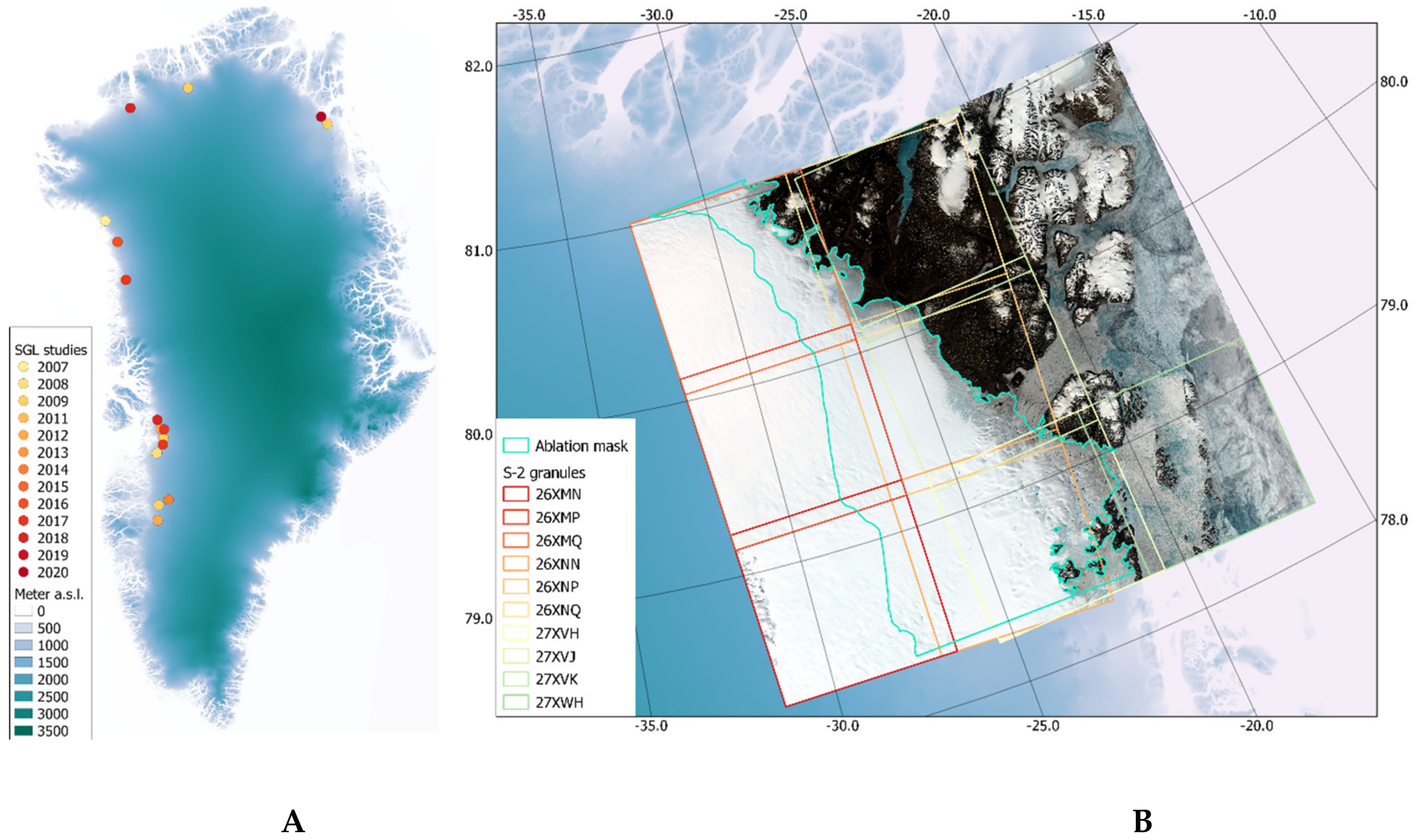
(A): Overview of SGL studies on Greenland between 2007 and 2020 [5,13,15,16,17,18,19,20,21,22,23,24,25,26,27,28]. Studies are color-coded by the year of publication. In case no exact coordinates were given in the respective study or a large area was monitored, the point was approximated to the center of the area of interest. In the case of multiple publications of the same first author for the same area of interest, only the first publication is shown. Studies covering the whole ice sheet, e.g., [29], are not shown. (B): Area of this study with footprints of the S-2 granules and the ablation mask used. True-color image is a 4–3–2 band mosaic of 19 June 2019. Background elevation model: Greenland Ice Sheet Mapping Project (GIMP) [30].
Figure 1.
(A): Overview of SGL studies on Greenland between 2007 and 2020 [5,13,15,16,17,18,19,20,21,22,23,24,25,26,27,28]. Studies are color-coded by the year of publication. In case no exact coordinates were given in the respective study or a large area was monitored, the point was approximated to the center of the area of interest. In the case of multiple publications of the same first author for the same area of interest, only the first publication is shown. Studies covering the whole ice sheet, e.g., [29], are not shown. (B): Area of this study with footprints of the S-2 granules and the ablation mask used. True-color image is a 4–3–2 band mosaic of 19 June 2019. Background elevation model: Greenland Ice Sheet Mapping Project (GIMP) [30].

Figure 2.
Flowchart of the data and methods applied. Rounded rectangles are input data; gray rectangles are processes, and blue parallelograms (intermediate) output.
Figure 2.
Flowchart of the data and methods applied. Rounded rectangles are input data; gray rectangles are processes, and blue parallelograms (intermediate) output.

Figure 3.
Postprocessing steps visualized by data of date 5 August 2019: (a) natural-color image (RGB, bands 4–3–2); (b) binary mask after thresholding; (c) binary mask cropped to the ablation area; (d) cropped mask after topographic shadow correction; (e) polygonized binary mask (with automatically created bounding box); (f) polygonized mask after dissolving; (g) lake polygons after cropping with topographic sinks; (h) lake polygons (g) over the true-color image (a).

Figure 4.
Sample statistics (dark) versus the whole dataset (bright): (A) number of sample scenes per year compared to the total number of scenes per year; numbers above bars indicate sample number (total number); (B) distribution of lake sizes for the whole dataset; (C) same as (B), only for the sample dataset.

Figure 5.
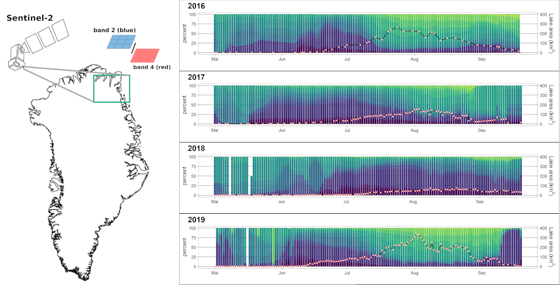
(A) Time-series of S-2 derived lake area sums for 2016, 2017, 2018 and 2019; (B) median lake area per 100 m altitude bin. Dot size: number of lakes per altitude and year.
Figure 5.
(A) Time-series of S-2 derived lake area sums for 2016, 2017, 2018 and 2019; (B) median lake area per 100 m altitude bin. Dot size: number of lakes per altitude and year.

Figure 6.
Lake area by elevation bins of 100 m as a percent of the total lake area per date between 1 May and 20 September (colored slices). Red dots show total lake area in km2. Values between observations (red dots) interpolated using linear regression.
Figure 6.
Lake area by elevation bins of 100 m as a percent of the total lake area per date between 1 May and 20 September (colored slices). Red dots show total lake area in km2. Values between observations (red dots) interpolated using linear regression.

Figure 7.
SGL distribution for the dates of maximum lake extent 2016 (24 July), 2017 (3 August), 2018 (21 August) and 2019 (2 August), plotted over ArcticDEM superimposed by an S-2 band 4–3–2 mosaic of 19 June 2019. Bottom panel: lake area for the same dates, summed upper 100 m elevation bin, versus the distance from the grounding line (colored lines). Black line: surface height of 79 N Glacier in m a.s.l.

Figure 8.
Comparison example of cloud masking procedures for 3 July 2017 (a,c,e,g,i) and 7 July 2017 (b,d,f,h,j): a,b: true-color image (band combination 4–3–2) of granule 26XNP; c,d: native level 1C cloud mask; e,f: fmask with default configuration; g,h: level 2A cloud mask (20 m resolution);i,j: results from the cloud classification matrix applied to the sink mask over the same granule. Labeled in pink are sinks where no lake was detected, purple are sinks where initially water was detected but was labeled as cloud/cloud covered, and yellow are sinks where lakes were detected and not labeled as cloudy.

Figure 9.
(A) lakes classified as cloud-covered using our algorithm versus cloud cover by level-1C (L1C) cloud mask, fmask and L2A cloud mask; (B) lakes classified as cloud-free using our algorithm versus the aforementioned masks. Axes display the number of lakes per scene and day. Right corners: root-mean-squared errors (RMSE) between the respective cloud masks and a perfect fit (dashed line).

Figure 10.
Rapid drainage event between 20 July 2017 and 26 July 2017. (A): S-2 true-color images of each day within the period, overlaid by the lake mask for the day in question (green = flagged as cloud-free, red-flagged as cloudy). (B): detected lake size in km2 before (blue) and after (purple) cloud detection (left vertical axis), and flags of cloud detection by time-dependent visibility (green) and spatial cloud extent (yellow, right vertical axis).

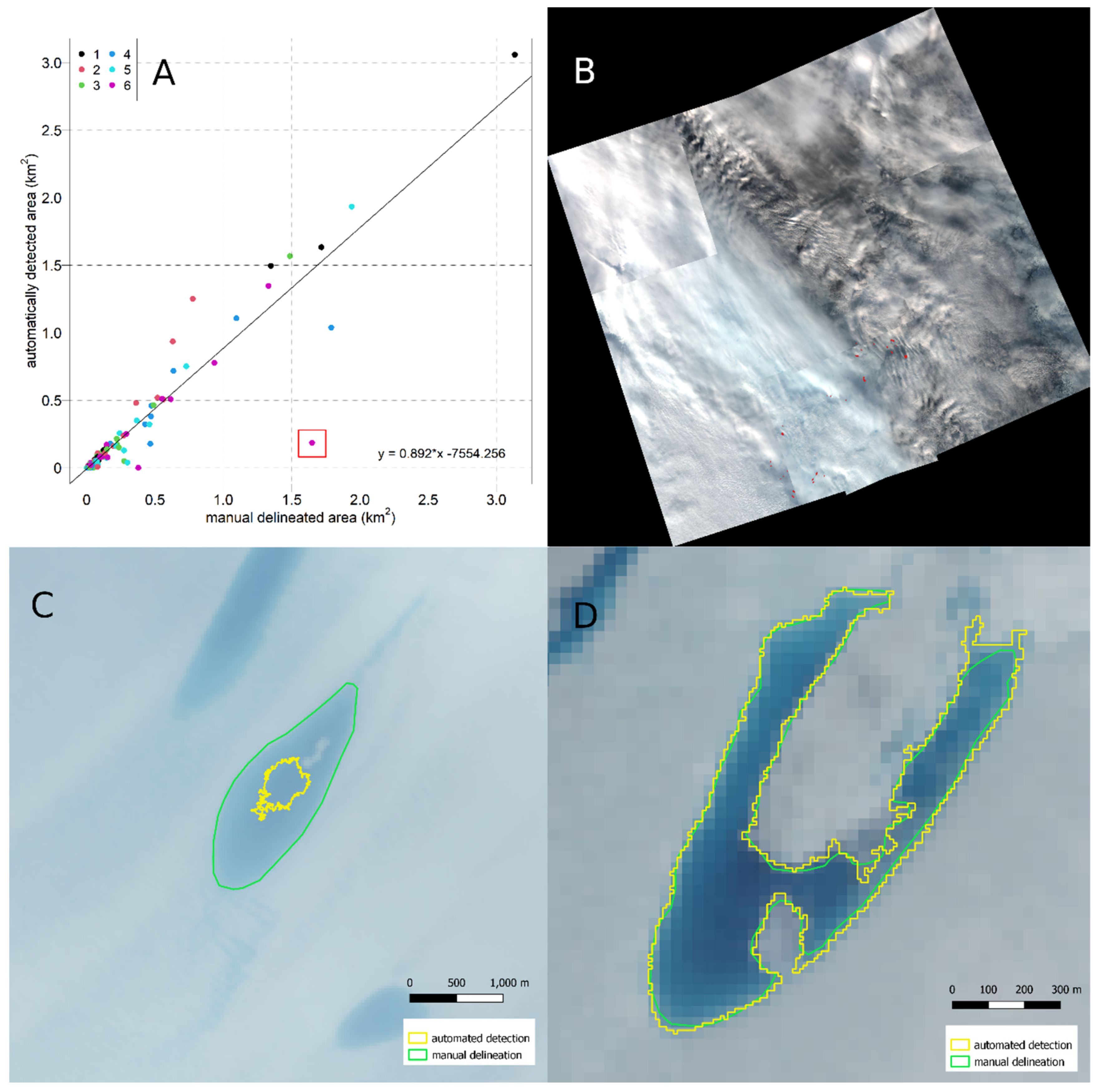
Figure 11.
Comparison of automatically detected and manually digitized lakes. (A) Linear regression (solid line) of manually (x-axis) and automatically (y-axis) derived lake areas. Point colors display cloud classes. Red rectangle: outlier lake (sink number 1020 of 1035) of date 17 August 2019. (B) RGB composite of date 17 August 2019, classified as extremely cloudy (class 6). (C) RGB closeup of the outlier (lake 1020, 30 m resolution) on the same date, with manually delineated extent (green) and automatically detected extent (yellow). (D) Difference between pixel-based (yellow) versus manual (green) delineation for lake 684, date 29 July 2018.


Table 1.
Multispectral sensors employed in previous studies of supraglacial lakes (SGL) on Greenland.
Table 1.
Multispectral sensors employed in previous studies of supraglacial lakes (SGL) on Greenland.
| Satellite | Sensor | Visible Spectra Resolution (m/Pixel) | Revisit Time in Days (at 79 N) | Cost | Swath Width (km) |
|---|---|---|---|---|---|
| Aqua/Terra | MODIS | 250 | daily | free of charge | 2330 |
| Landsat 7/8 | ETM+/OLI | 30 | 16 | free of charge | 185 |
| WorldView 2/3 | WV-3 Imager | 0.3 | daily | Commercial—price per km2 1 | 13.1 |
| Terra | ASTER | 15 | 16 | free of charge | 60 |
| Sentinel-2 | MSI | 10 | ca. 1.5 days | free of charge | 290 |
1 pricing varies with respect to provider, archive/new acquisition, or processing level.
Table 2.
S-2 data coverage by year, with day of the year (DOY) 1 as the day of the first complete set for the respective year and DOY n as the last day with a complete scene set.
Table 2.
S-2 data coverage by year, with day of the year (DOY) 1 as the day of the first complete set for the respective year and DOY n as the last day with a complete scene set.
| Year | DOY 1 | DOY n | Complete Scenes | Average Interval (Days) |
|---|---|---|---|---|
| 2016 1 | 93 | 262 | 54 | 3.13 |
| 2017 | 86 | 262 | 106 | 1.66 |
| 2018 | 82 | 263 | 150 | 1.21 |
| 2019 | 77 | 263 | 169 | 1.10 |
1 S-2 A only, due to the start of S-2 B in March 2017.
Table 3.
Lake area characteristics per year. If there is still > 1 km2 of lake area at the end of the sensing period, the melt season end cannot be determined (-).
Table 3.
Lake area characteristics per year. If there is still > 1 km2 of lake area at the end of the sensing period, the melt season end cannot be determined (-).
| Year | Max Lake Area (km2) | Date of Max Lake Area (DOY) | Start of Melt Season (DOY) | End of Melt Season (DOY) |
|---|---|---|---|---|
| 2016 | 265.39 | 24 July (206) | 10 June (162) | 19 September (263) |
| 2017 | 153.26 | 3 August (215) | 23 May (143) | - |
| 2018 | 76.66 | 21 August (233) | 13 June (164) | - |
| 2019 | 333.19 | 2 August (214) | 6 June (157) | 18 September (261) |
Publisher’s Note: MDPI stays neutral with regard to jurisdictional claims in published maps and institutional affiliations. |
© 2021 by the authors. Licensee MDPI, Basel, Switzerland. This article is an open access article distributed under the terms and conditions of the Creative Commons Attribution (CC BY) license (http://creativecommons.org/licenses/by/4.0/).
Share and Cite
MDPI and ACS Style
Hochreuther, P.; Neckel, N.; Reimann, N.; Humbert, A.; Braun, M. Fully Automated Detection of Supraglacial Lake Area for Northeast Greenland Using Sentinel-2 Time-Series. Remote Sens. 2021, 13, 205. https://doi.org/10.3390/rs13020205
AMA Style
Hochreuther P, Neckel N, Reimann N, Humbert A, Braun M. Fully Automated Detection of Supraglacial Lake Area for Northeast Greenland Using Sentinel-2 Time-Series. Remote Sensing. 2021; 13(2):205. https://doi.org/10.3390/rs13020205
Chicago/Turabian StyleHochreuther, Philipp, Niklas Neckel, Nathalie Reimann, Angelika Humbert, and Matthias Braun. 2021. "Fully Automated Detection of Supraglacial Lake Area for Northeast Greenland Using Sentinel-2 Time-Series" Remote Sensing 13, no. 2: 205. https://doi.org/10.3390/rs13020205
Note that from the first issue of 2016, this journal uses article numbers instead of page numbers. See further details here.