Characteristics of the Bright Band Based on Quasi-Vertical Profiles of Polarimetric Observations from an S-Band Weather Radar Network

Weather Radar Center, Korea Meteorological Administration, Seoul 07062, Korea
*
Author to whom correspondence should be addressed.
Remote Sens. 2020, 12(24), 4061; https://doi.org/10.3390/rs12244061
Submission received: 20 November 2020
/
Revised: 4 December 2020
/
Accepted: 7 December 2020
/
Published: 11 December 2020
(This article belongs to the Special Issue Radar-Based Studies of Precipitation Systems and Their Microphysics)
Abstract
:Bright band (BB) characteristics obtained via dual-polarization weather radars elucidate thermodynamic and microphysical processes within precipitation systems. This study identified BB using morphological features from quasi-vertical profiles (QVPs) of polarimetric observations, and their geometric, thermodynamic, and polarimetric characteristics were statistically examined using nine operational S-band weather radars in South Korea. For comparable analysis among weather radars in the network, the calibration biases in reflectivity (ZH) and differential reflectivity (ZDR) were corrected based on self-consistency. The cross-correlation coefficient (ρHV) bias in the weak echo regions was corrected using the signal-to-noise ratio (SNR). First, we analyzed the heights of BBPEAK derived from the ZH as a function of season and compared the heights of BBPEAK derived from the ZH, ZDR, and ρHV. The heights of BBPEAK were highest in the summer season when the surface temperature was high. However, they showed distinct differences depending on the location (e.g., latitude) within the radar network, even in the same season. The height where the size of melting particles was at a maximum (BBPEAK from the ZH) was above that where the oblateness of these particles maximized (BBPEAK from ZDR). The height at which the inhomogeneity of hydometeors was at maximum (BBPEAK from the ρHV) was also below that of BBPEAK from the ZH. Second, BB thickness and relative position of BBPEAK were investigated to characterize the geometric structure of the BBs. The BB thickness increased as the ZH at BBBOTTOM increased, which indicated that large snowflakes melt more slowly than small snowflakes. The geometrical structure of the BBs was asymmetric, since the melting particles spent more time forming the thin shell of meltwater around them, and they rapidly collapsed to form a raindrop at the final stage of melting. Third, the heights of BBTOP, BBPEAK, and BBBOTTOM were compared with the zero-isotherm heights. The dry-temperature zero-isotherm heights were between BBTOP and BBBOTTOM, while the wet-bulb temperature zero-isotherm heights were close to the height of BBPEAK. Finally, we examined the polarimetric observations to understand the involved microphysical processes. The correlation among ZH at BBTOP, BBPEAK, and BBBOTTOM was high (>0.94), and the ZDR at BBBOTTOM was high when the BB’s intensity was strong. This proved that the size and concentration of snowflakes above the BB influence the size and concentration of raindrops below the BB. There was no depression in the ρHV for a weak BB. Finally, the mean profile of the ZH and ZDR depended on the ZH at BBBOTTOM. In conclusion, the growth process of snowflakes above the BB controls polarimetric observations of BB.
1. Introduction
When falling snowflakes pass through the zero-isotherm layers into the warmer air, they melt and collapse to form raindrops, causing an increase in radar reflectivity (known as the bright band, hereafter BB). The reflectivity (ZH) increases owing to the increase in the dielectric constant. Afterwards, the ZH decreases upon the formation of raindrops, owing to the decrease in the size and number concentration of snowflakes caused by the increase in fall velocity [1,2]. The overestimation in ZH causes a significant error in radar rainfall estimates under the BB region. The identification of BB and correction of related errors are necessary for accurate estimations of precipitation [3,4,5]. The study of the vertical structure of the precipitation system associated with the melting layer and its characteristic analysis using remote sensing instruments is essential to understand cloud physics and rain microphysics. Weather radar can provide crucial information on melting layers with high spatiotemporal resolution. Therefore, detection and characterization of the BB using weather radar is one of the primary keys for understanding the microphysical processes related to the vertical structure of precipitation.
Most single-polarimetric techniques have identified the BB (i.e., peak, top, and bottom) based on a geometric feature from the vertical profile of ZH (VPR) [1,6,7,8,9,10]. The gradient of VPR has been commonly used to define the boundary of BB. Klaassen [11] and White et al. [12] used the change in radial velocity when snowflakes turn into raindrops as they pass through the melting layer to identify the BB. Dual-polarization radar can provide information on the size, shape, and phase of hydrometeors, resulting in improved BB detection [13,14,15,16,17]. Ryzhkov and Zrnić [13] showed that polarimetric signatures pronounce the presence of BB. Brandes and Ikeda [14] identified BB by matching observed and modelled profiles of polarimetric observations. Giangrande et al. [16] proposed thresholds for ZH, the differential reflectivity (ZDR), and the cross-correlation coefficient (ρHV) to detect top and bottom boundaries of BB in an operational environment. Boodoo et al. [18] modified the technique developed by Giangrande et al. [16] for a C-band radar in southern Ontario, Canada. The top of the BB effectively matched the 0 °C wet-bulb temperature layer. Illingworth and Thompson [19] showed that the linear depolarization ratio (LDR) was valuable for identifying BB and correcting an increase in ZH due to BB. Hall et al. (2015) developed a fuzzy logic-based BB detection technique using ZH, ZDR, ρHV, and LDR.
Fabry and Zawadzki [1] analyzed the vertical structure of BB revealed by X-band vertically pointing radar and wind profiler. The intensity of BB depends on variations in the refractive index, shape, and density of hydrometeors. Zawadzki [20] developed a BB model that showed that dense particles reduce the difference in ZH at the peak height of the BB and in the rain region. Wolfensberger et al. [21] analyzed the characteristics of BB using the range-height indicator (RHI) scan mode at various climatic regions (i.e., South of France; Swiss Alps and plateau; and Iowa, USA). The distribution of polarimetric observations within the BB was similar regardless of the season and climatic regions. They also showed that the thickness of BB is highly related to the presence of rimed particles, the fall velocity of the hydrometeors, and BB intensity.
Recently, quasi-vertical profiles (QVPs) of polarimetric observations (described in more detail in Section 3) were used to investigate the vertical structure and microphysical processes of the precipitation system [22,23,24,25]. Kumjian et al. [22] first used QVP to detect refreezing signals of precipitation during winter storms. According to Ryzhkov et al. [24], QVP is a useful tool for the examination of microphysical processes resulting in precipitation on the surface and aids in the determination of the growth process of snowflakes. Kumjian and Lombardo [23] analyzed the microphysical and dynamic characteristics of winter snowstorms. They found that an increase in differential reflectivity (ZDR) represented the initial stage of planar crystal growth, and an increase in the specific differential phase (KDP) indicated the high number concentrations of planar crystals. The supersaturation caused by the ascent boosts the depositional growth and raises the potential of an increase in KDP. Trömel et al. [26] showed the potential of ground precipitation nowcasting by identifying microphysical processes of stratiform snowfall storms. The KDP increase in the dendritic growth layer (DGL, between −10 and −20 °C) exhibited a very high correlation with rainfall on the ground after half an hour. Griffin et al. [27] detected BB and analyzed the microphysical processes associated with BB and DGL for stratiform precipitation in winter. Using the QVPs of polarimetric observations, they identified a weak BB (ZH of < 20 dBZ) whose detection failed when using the vertical profile of ZH only. They also compared polarimetric observations above, within, and below the BB using QVPs for the first time at the S band.
In this study, we identified BB using the QVPs of polarimetric observations obtained from nine S-band dual-polarization radars operated by the Korea Meteorological Administration (KMA). For the analysis of BB characteristics, geometric features (including heights of the BB peak, top, and bottom at QVPs) were analyzed statistically, and then compared to the height of the 0 °C isotherm. Finally, the characteristics of polarimetric observations at the top, peak, and bottom of the BB were examined to determine the microphysical processes related to the BB.
2. Materials and Methods
2.1. Materials and Data
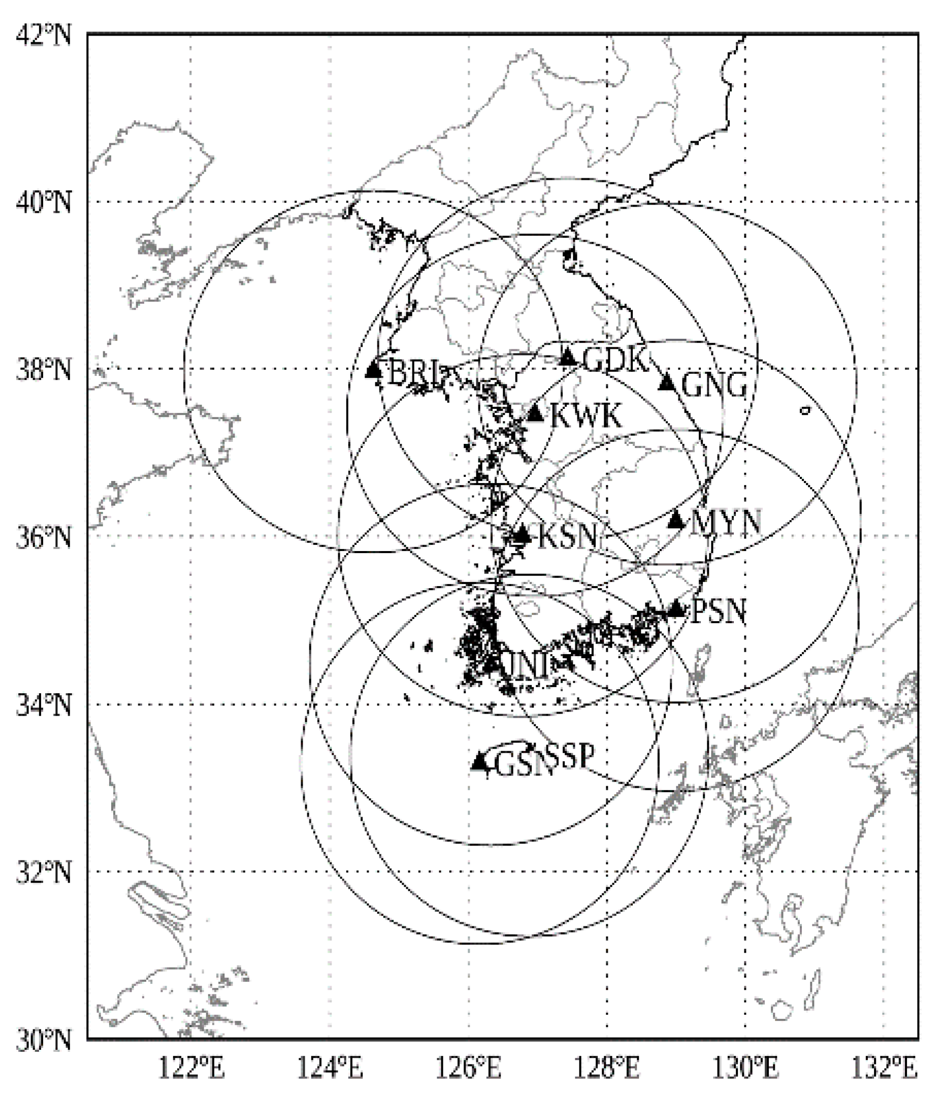
The KMA has operated a nationwide weather radar network composed of 10 S-band weather radars since 2008 and sequentially replaced all radars of the network with S-band dual-polarization radars during the period from 2014 to 2019. Figure 1 shows the deployment of the KMA S-band dual-polarization weather radar. The replacement began with the BRI radar at the northwestern island in 2014 and ended with the GNG radar at the northeastern coast in November 2019. We used a total of nine weather radars, except for the GNG radar, to analyze the characteristics of the BB from March to November 2019. Table 1 shows the volumetric scan strategies of the weather radar in the KMA network. All strategies consisted of nine elevation angles, including a wind profiling mode of 15° and were repeated every 5 min. Notably, several radars (i.e., KWK, MYN, and PSN) installed at a relatively high altitude (>600 m mean sea level (MSL)) employed a negative (−) elevation as the lowest elevation angle. The elevation angles for the lowest scan were determined based on a radar beam blockage simulation for standard beam propagation using the digital elevation model with a horizontal resolution of 1 arc second. The radar transmits a long pulse with a width of 2 μs at low elevation angles (less than 3°) to enhance the detectability of weak low-level echoes, such as winter snowstorms, whereas a short pulse of 1 μs pulse width is used at higher elevation angles (>3°) to increase the Nyquist velocity using high pulse repetition frequency (PRF). This configuration of the pulse length is based on the sensitivity test by Lee et al. [28]. They found that a longer pulse length (i.e., 2 μs) improved radar sensitivity and increased the spatial extent of the precipitation echo for radar reflectivity and all dual-polarimetric observations. The azimuthal and radial resolutions were 1.0° and 250 m, regardless of the elevation angle. The BB was identified using QVPs of polarimetric observations at the highest elevation angle of 15.0°.
To analyze the thermodynamic characteristics of BB, three-dimensional dry-bulb temperature (T), dew point temperature (Td) and wet-bulb temperature (Tw) data from three-dimensional atmospheric fields (T, Td, and pressure) were generated by multi-quadric interpolation using observational data and very short-range data assimilation and prediction systems (VDAPS) [29] were used every 5 min. The horizontal resolution of three-dimensional atmospheric field data was 4 km, and the vertical resolution was 100 m at altitudes of 0–2 km and 200 m at altitudes of 2–10 km. The three-dimensional data consisted of 60 × 257 × 257 (10 km × 1024 km × 1024 km) grids. The temperature data was interpolated to the same vertical resolution of the QVPs (20 m).
2.2. Methodology
2.2.1. Construction of the QVPs
The QVPs were obtained by azimuthal averaging individual polarimetric observations at each range gate and for the highest elevation angle (15°). According to Ryzhkov et al. [24], the QVP at an elevation angle between 10 and 20° can reduce horizontal inhomogeneity. The QVP provides a stable vertical structure of the precipitation system for the BB identification, where ZH and ZDR increase and ρHV decreases.
Two kinds of corrections were required for all KMA radars before constructing the QVPs of polarimetric observations as follows: (1) the calibration biases in the power-based polarimetric measurements (i.e., ZH and ZDR) and (2) the correction of ρHV in the low SNR area. First, the calibration biases in ZH and ZDR lead to an unsuitable identification of the BB, and the different calibration biases among radars within the network resulted in a misunderstanding of the spatial and temporal statistics of BB. In this study, the ZH bias was corrected based on the self-consistency principle between ZH and differential phase (ΦDP) [30,31]. The ZDR bias was calibrated by comparing the empirical relationship between ZH and ZDR obtained from the drop size distribution of a two-dimensional video disdrometer (2DVD) to the ZH-ZDR distribution of polarimetric measurements. Kwon et al. [31] described these two procedures in detail.
The noise caused by a radar receiver, waveguide, and antenna affects the quality of the polarimetric observations, even if the radar is properly calibrated [32]. The ρHV is biased in the low signal-to-noise ratio (SNR) areas. Meteorological echoes with a ρHV less than 0.98 are observed due to the bias related to the noise. The ρHV was corrected using the SNR as follows:
where ρHV(m) and ρHV are the measured and corrected ρHV, respectively. The snr (=100.1SNR(dB)) is the SNR in linear units.
ρHV = ρHV(m) (1 + 1/snr)
Radar observations included non-meteorological echoes. The regions with ρHV < 0.7, or with SNR < 10 dB, were removed to avoid contamination by non-meteorological echoes. The QVPs of polarimetric observations were constructed by obtaining the azimuthal average of ZH, ZDR, and ρHV. As the radar beam broadens, the QVP resolution is reduced at high altitudes. In this study, QVPs were converted to high resolution by interpolating them to a vertical resolution of 20 m. The QVPs of ZH, ZDR, and ρHV were used to analyze the characteristics of polarimetric observations at the top, peak, and bottom of the BB.
2.2.2. Detection of the Bright Band (BB)
Most BB detection algorithms apply the first and second derivatives of ZH (dZ/dh and d2Z/dh2). However, local variations of ZH can make the detection of the boundary of the BB challenging. A sharp curvature of ZH is required for the detection of the top and bottom of the BB. The coordinate rotation method developed by Rico-Ramire and Cluckie [9] was used to detect the boundaries of the BB. This method is simple and has the advantage of reliably detecting the BB signature,.The ZH and ZDR increase due to the increase in the hydrometeor dielectric constants and densities, and the ρHV decreases due to the diversity of the hydrometeor shapes, orientations, and densities. Before applying the coordinate rotation method, the ρHV was normalized to a value ranging between 0 and 100, and then converted to a new variable (new ρHV = 100 − 100*ρHV), which increased in the BB as a result of this conversion.
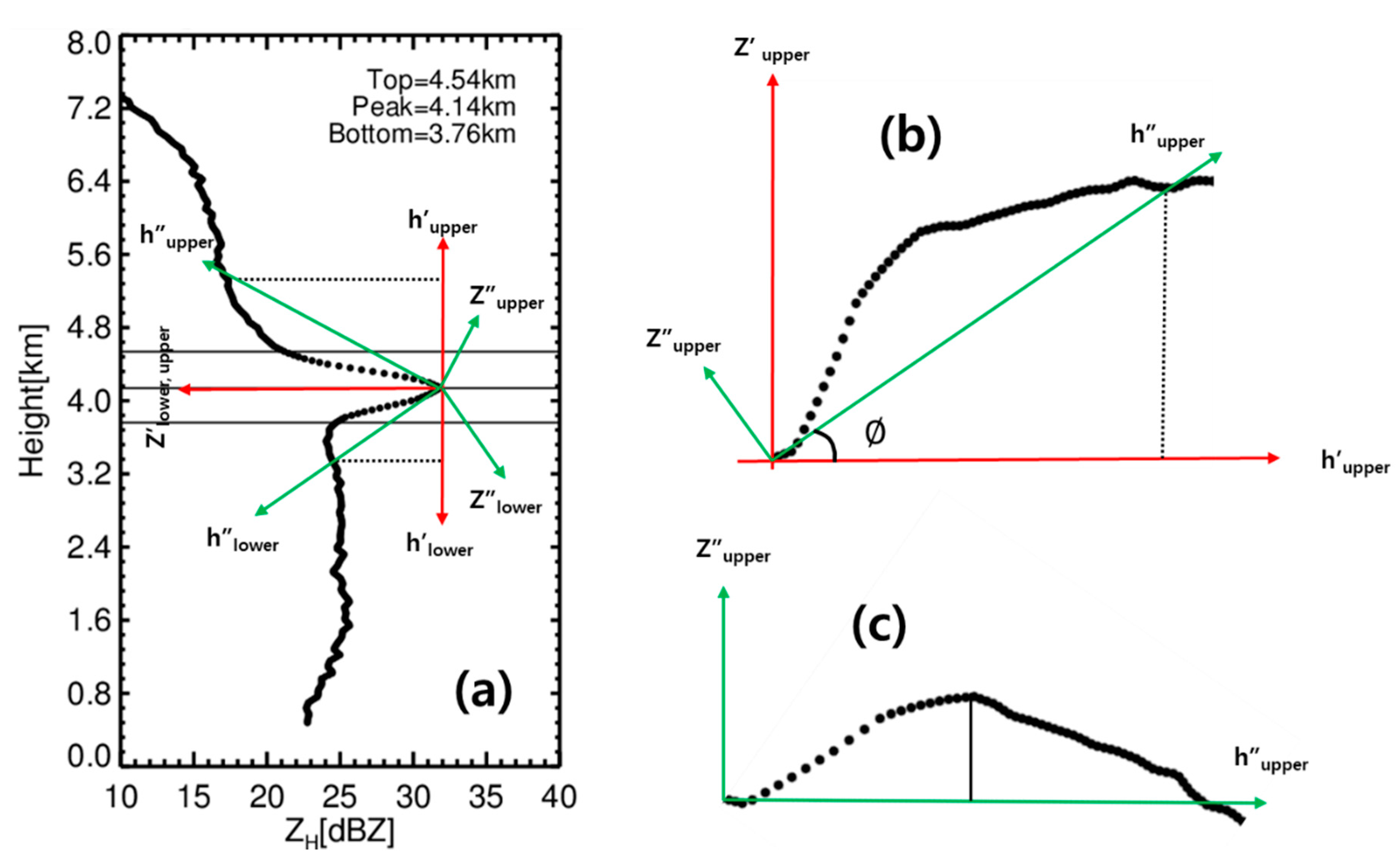
The procedures for BB detection using the QVPs of the ZH, ZDR, and new ρHV were divided into the following two steps: (1) detection of the peak of the BB (BBPEAK) and (2) detection of the top and bottom of the BB (BBTOP and BBBOTTOM) using the coordinate rotation method. BBPEAK was identified by calculating the first derivative of polarimetric observations. The first derivative was calculated from the difference in the polarimetric observations at a height of 60 m above and below a given height. BBPEAK was obtained from the maximum polarimetric observations (ZH, ZDR, and new ρHV) within a height of 400 m above and below the height at which the first gradient was at maximum. The ZH, ZDR, and new ρHV at BBPEAK should be greater than 0.0 dBZ, 0.0 dB, and 2 (=0.98), respectively. In this study, we briefly describe the coordinate rotation method. Figure 2 shows a diagram of the procedures for detecting BBTOP and BBBOTTOM from the QVP of the ZH. First, the QVP was separated by the upper and lower parts of BBPEAK relative to the line connecting BBPEAK and Z′lower, upper. The original coordinate was rotated 90° in the clockwise (counterclockwise) direction to obtain the new coordinate with h′upper−Z′ upper (h′lower−Z′lower). Then, the height of 1200 m (800 m) above (below) BBPEAK was selected to set the rotation angle . The coordinate was again rotated degrees in the clockwise (counterclockwise) direction, and h″upper (h″lower) and Z″ upper (Z″lower) are the x-axis and y-axis in the final coordinate. The maximum value in the final coordinate was defined as BBTOP (BBBOTTOM).
Figure 3 shows the time series of the QVPs of the ZH (top), ZDR (middle), and ρHV (bottom), and the heights of BBTOP (blue), BBPEAK (black), and BBBOTTOM (red) at an elevation angle of 15° for the BRI radar from 000 KST of 6 September 2019 to 1800 KST of 7 September 2019. In Figure 3a,c,e, the black solid line indicates BB height and the black dotted lines indicate T with a 5 °C interval (ranging from −30 to 20 °C). BBPEAK is located at the ZH maxima, ZDR maxima, and ρHV minima. BBTOP and BBBOTTOM are within a height of 500 m above and below BBPEAK. In Figure 3b,d,f, the solid and dashed lines indicate the heights where T is 0 °C and Tw is 0 °C, respectively. The height of BBTOP is closer to the zero-isotherm layer (T = 0 °C) than that of BBPEAK and BBBOTTOM.
2.2.3. Variables for Characterizing the BB
The definitions of the feature parameters used to characterize the BB are presented in Table 2. These parameters are related to the geometric, thermodynamic, and polarimetric properties of the BB. The heights of the BB (BBTOP, BBPEAK, and BBBOTTOM) obtained by each polarimetric observation are H(ZH Top), H(ZH Peak), H(ZH Bottom), H(ZDR Top), H(ZDR Peak), H(ZDR Bottom), H(ρHV Top), H(ρHV Peak), and H(ρHV Bottom). H(T = 0 °C), H(Td = 0 °C), and H(Tw = 0 °C) are the heights where T, Td, and Tw are 0 °C. ZH Top, ZH Peak, ZH Bottom, ZDR Top, ZDR Peak, ZDR Bottom, ρHV Top, ρHV Peak, and ρHV Bottom, which are the polarimetric observations at the heights of BBTOP, BBPEAK, and BBBOTTOM were defined to analyze polarimetric characteristics in the BB.
3. Results and Discussion
3.1. Characterization of the BB
3.1.1. Height of the BB
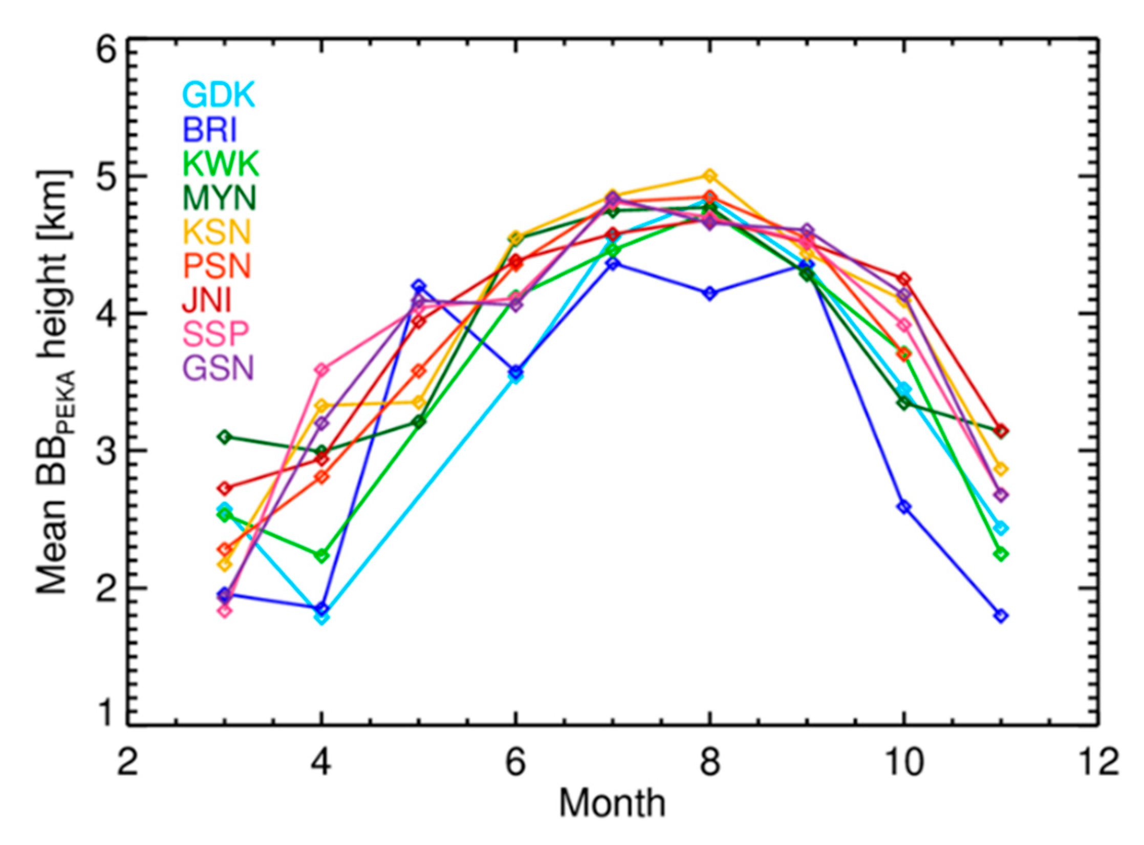
The monthly average H(ZH Peak) is shown in Figure 4 and Table 3. The cold (warm) color indicates that the radar is located at higher (lower) latitude. All H(ZH Peak) values in the warm season were higher than those in the cold season. The H(ZH Peak), which ranged from 4.14 to 4.71 km, on average, during the summer, showed an annual variation with a peak in July or August. The mean H (ZH Peak) in March, April, and November was less than 3.0 km, and that in September was greater than 4.0 km. The differences in H(ZH Peak) among radars during the cold seasons were greater than those during warm seasons. Overall, the H(ZH Peak) from radars at higher latitudes was lower than that from radar at lower latitudes. The H(ZH Peak) at the GSN and SSP radars, which are located at relatively low latitudes, reached 4 km in May, whereas those at the KWK, MYN, KSN, PSN, and JNI radars exceeded 4 km in June. The H(ZH Peak) at the BRI and GDK radars, which are located at relatively high altitudes, exceeded 4 km in July.
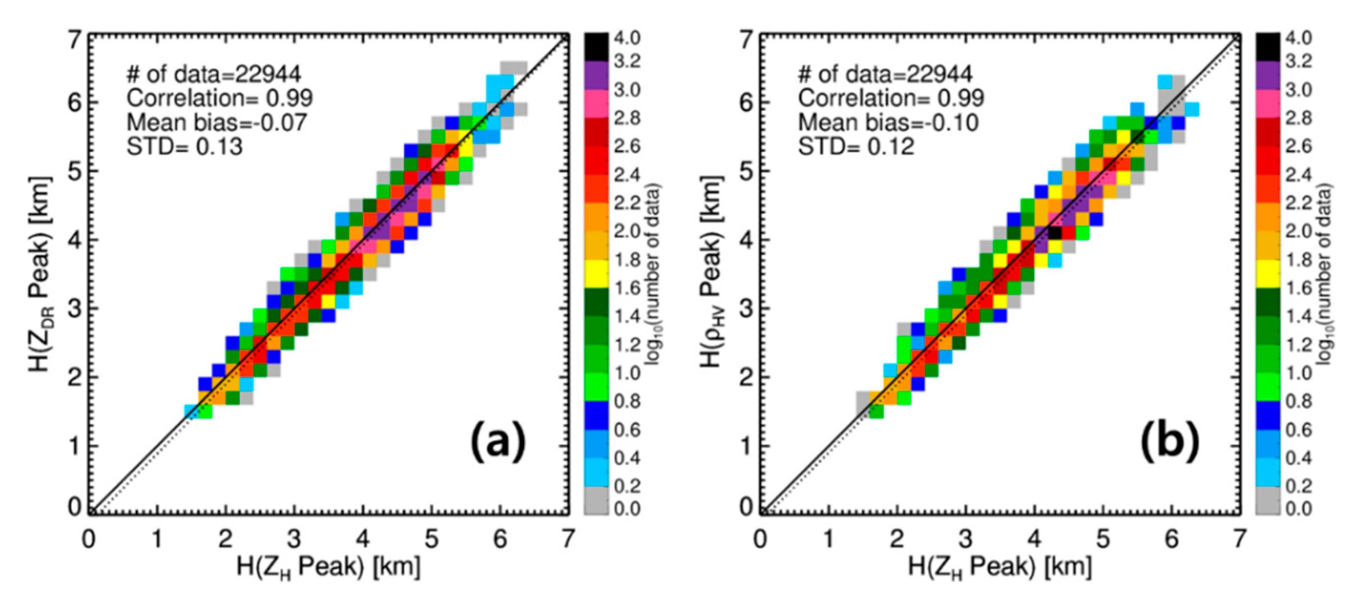
Figure 5 shows the two-dimensional frequency distribution between H(ZDR Peak) and H(ZH Peak) and between H(ρHV Peak) and H(ZH Peak). H(ZH Peak) was 70 m and 100 m higher than H(ZDR Peak) and H(ρHV Peak), respectively. The ZH depends on the size, refractive index, and number concentration of hydrometeors in the melting layer. When the snowflakes enter the 0 °C isotherm layer, they start to melt at the tips of the crystal branches (mainly at the bottom side). Small snowflakes melt faster than large snowflakes, which boosts the aggregation and coalescence due to the difference in fall velocity. The ZH increase below the 0 °C isotherm layer is due to the increase in the particle size (aggregation) or number density (no aggregation). The maximum of the ZH results from melting particles covered by meltwater with a large size and a high dielectric constant. The fall velocity increases as large particles turn into raindrops below ZH Peak. This process reduces the ZH due to a decrease in the number concentration. In the BB, the ZDR increases due to the oblate shape of the melting particles. The oblateness of the particles is maximized below ZH Peak (where their size is at maximum). The decrease in the ZDR below the BB is due to the break-up of large melted snowflakes, since the ZDR is not related to the number concentration. The ρHV begins to decrease when the snowflakes and raindrops mix to a sufficient degree; therefore, it occurs at a relatively lower altitude than where the ZH starts to increase via melting [16,21]. In other words, the ZH depends on the change in size and number concentration of melting snowflakes, whereas the ZDR and ρHV are subject to the non-spherical shape of melting snowflakes. The mean height difference between BBPEAK from the ZH and ρHV was 100 m in this study, which is consistent with the heights of 90, 96, and 121 m obtained in previous studies [21,33,34]. BB detection based on the ρHV can cause the underestimation of the height of the BB, as mentioned by Wolfensberger et al. [21]. According to Trömel et al. [26], the height of the maximum ZH was very close to that of the maximum backscatter differential phase (δ) and was higher than that of the minimum ρHV. Trömel et al. [26] suggested that differences between heights should be analyzed in various climatic conditions to determine whether the aforementioned phenomenon is caused by differences in microphysical processes.
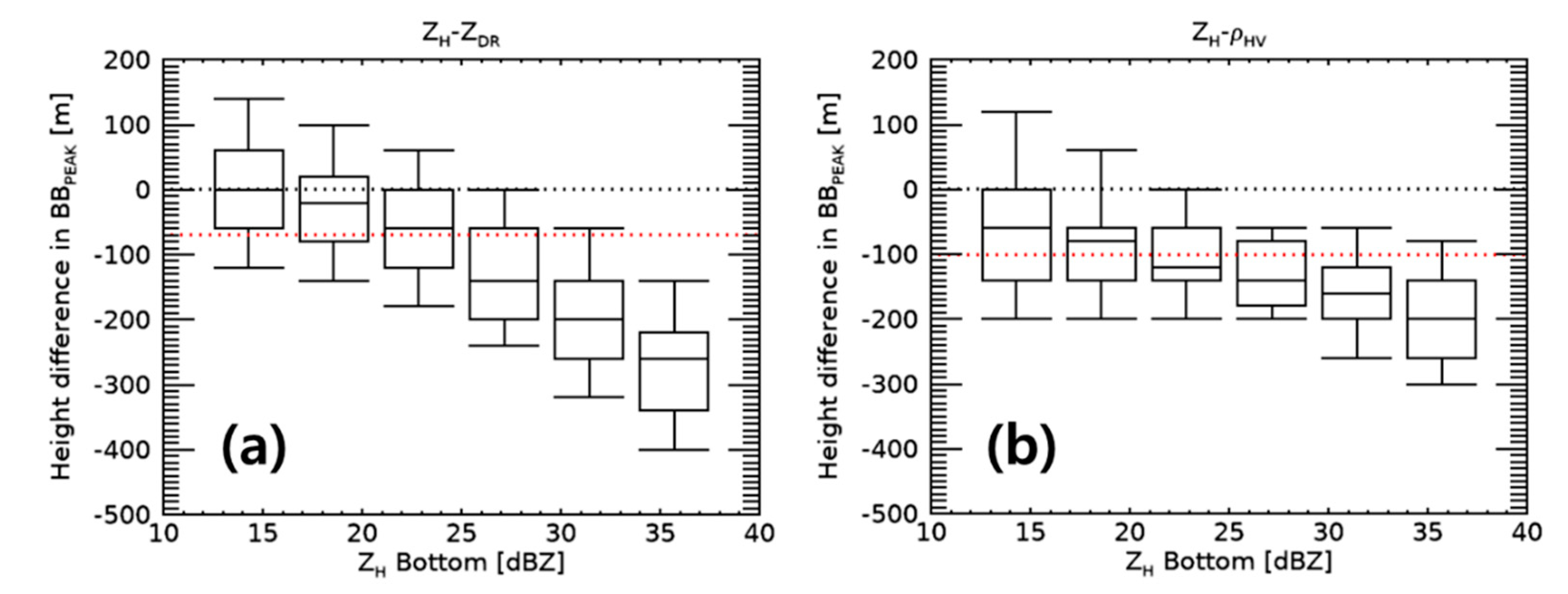
Figure 6 shows the difference between H(ZH Peak) and H(ZDR Peak) (black line), and that between H(ZH Peak) and H(ρHV Peak) (red line) as a function of ZH Bottom. The black (red) dotted line indicates no difference (the mean difference in heights shown in Figure 5). H(ZDR Peak) was almost identical to H(ZH Peak) in the range of 10 to 15 dBZ, whereas it was lower than 290 m than H(ZH Peak) in the range of 35 to 40 dBZ. However, H(ρHV Peak) differed from H(ZH Peak) by more than 60 m (200 m) in the range of 10 to 15 dBZ (35 to 40 dBZ). In summary, according to Figure 5 and Figure 6, H(ZH Peak), H(ZDR Peak), and H(ρHV Peak) did not match. The difference in heights of BBPEAK increased with increasing ZH Bottom. The larger size and higher number concentration of melting snowflakes result in more significant differences in the height of BBPEAK based on polarimetric observations.
3.1.2. Geometric Structure of the BB
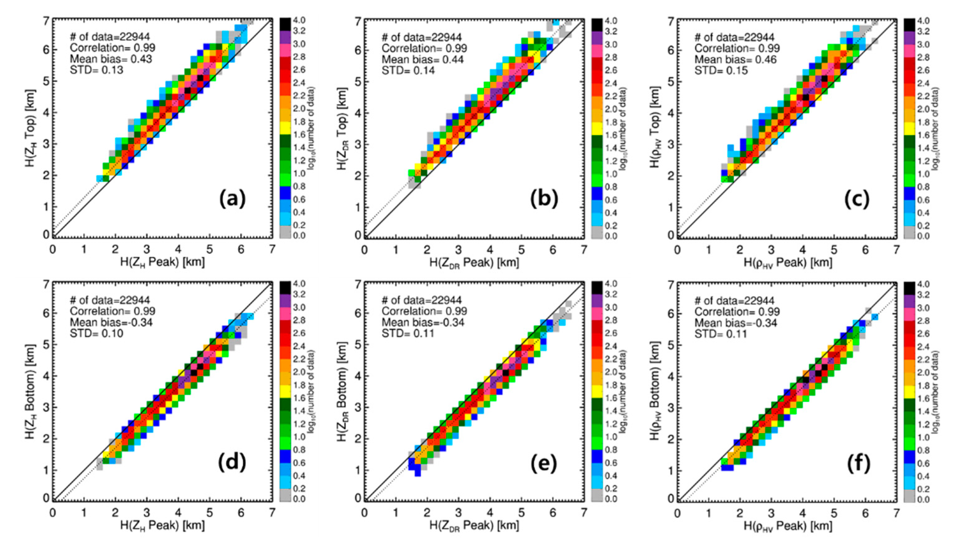
The heights of BBTOP, BBPEAK, and BBBOTTOM were analyzed to characterize the vertical structure of the BB. Figure 7 shows the frequency distributions among the heights of BBTOP, BBBOTTOM, and BBPEAK for ZH, ZDR, and ρHV, respectively. BBTOP was 430–460 m higher than BBPEAK, and BBBOTTOM was 340 m lower than BBPEAK on average, indicating that the structure of the BB was asymmetric. Physically, the melting particles spend more time covering the thin shell of meltwater around them, while they rapidly collapse to form a raindrop at the final stage of melting. The difference between the heights of BBTOP and BBBOTTOM is considered to be the BB thickness, and the relative position (r) is considered to be the difference between the heights of BBPEAK and BBBOTTOM to the BB thickness as expressed below:
r = (H(BBPEAK) − H(BBBOTTOM))/BB thickness
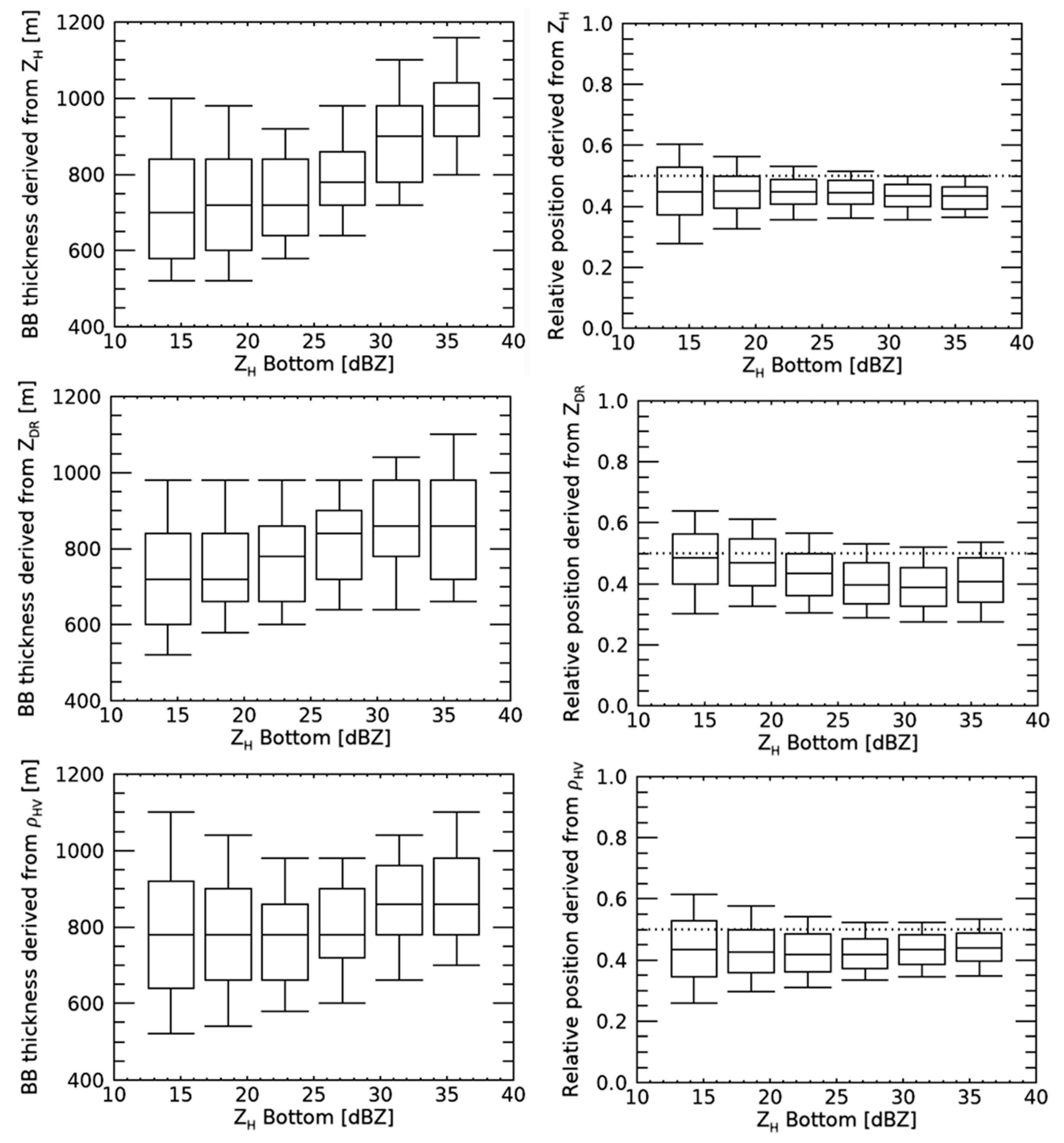
Figure 8 shows box plots of the BB’s thickness (left) and r (right) according to ZH Bottom at intervals of 5 dB. For the ZH and ZDR, the thicknesses of the BB increased with increasing ZH Bottom. The weak ZH in the BB represents non-aggregated snowflakes that are small in size. On the one hand, small snowflakes melt quickly and result in a thin BB. On the other hand, heavily aggregated snowflakes cause a thick and strong BB due to the fact that they need more time to completely melt than small particles. Interestingly, the BB thickness slowly increased until 20 dBZ, and rapidly increased above 20 dBZ, as shown in [34]. The BB thickness estimated using the ZH and ZDR exceeded 980 m and 870 m in the 35–40 dBZ range of ZH Bottom. The BB thickness estimated using ρHV was 800 m in the 10–15 dBZ range of ZH Bottom and 875 m in the 35–40 dBZ range of ZH Bottom. The ρHV related to the diversity of hydrometeors had a relatively constant thickness regardless of ZH at BBBOTTOM and a smaller variation as compared with the ZH and ZDR. The r was 0.45 for the ZH and ρHV regardless of ZH Bottom, and BBPEAK was closer to BBBOTTOM than BBTOP. The r of the ZDR decreased from 0.5 to 0.4 as ZH Bottom increased from the range of 10–15 dBZ to 35–40 dBZ. The non-symmetric structure of the ZDR resulted from a rapid decrease in the ZDR, due to the break-up of large melted particles at the final state of melting process [34].
3.1.3. Thermodynamic Characteristic of the BB
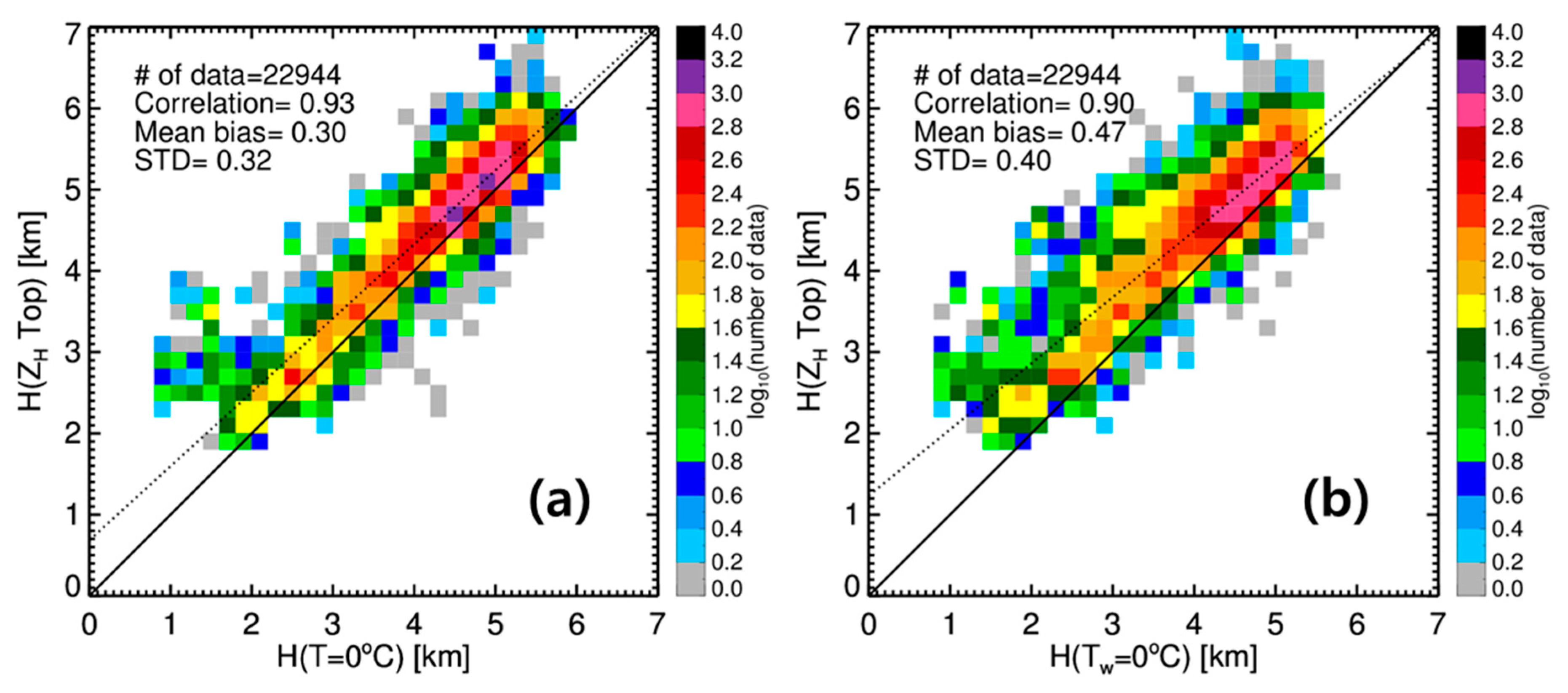
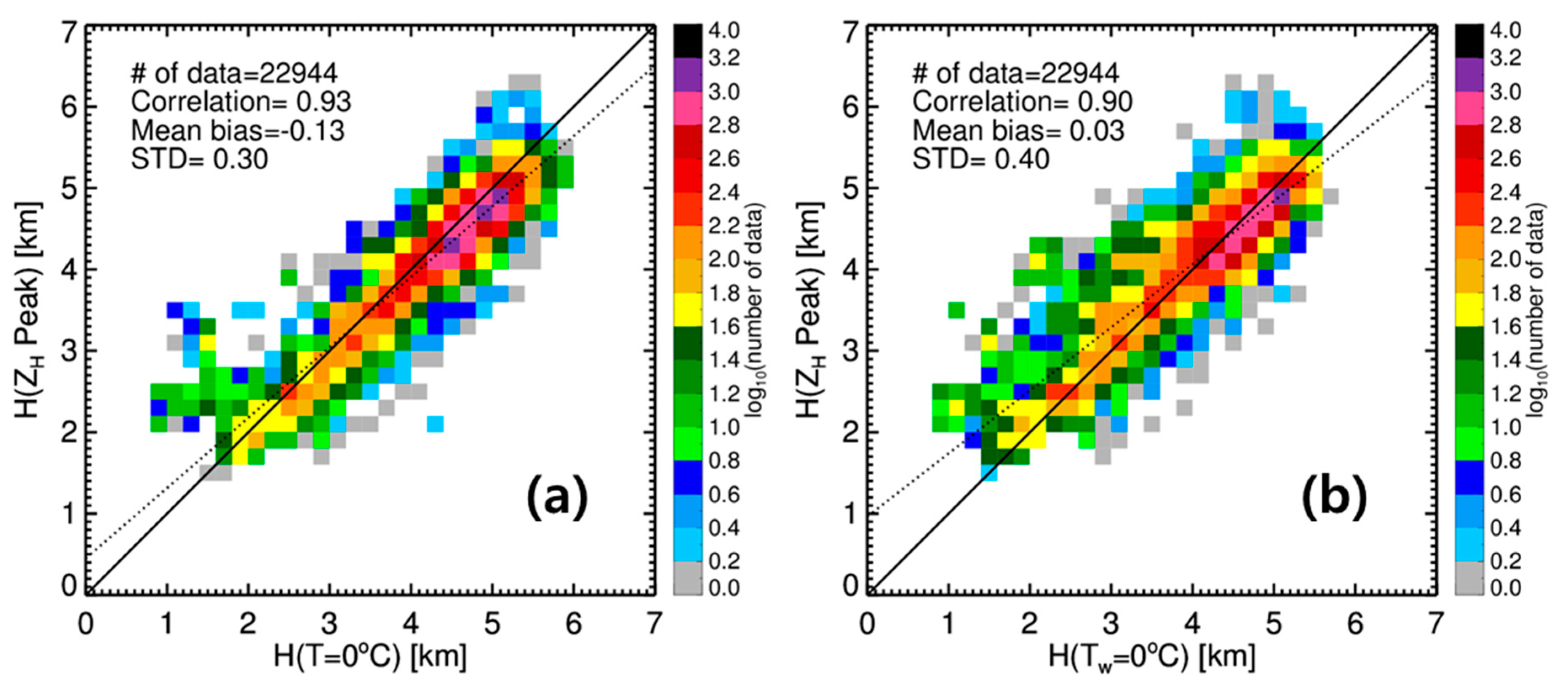
The seasonal variability of the height of the BB depends on the ground temperature. To further analyze the thermodynamic characteristics of the BB, we compared H (T = 0 °C), H (Tw = 0 °C), H(ZH Top), and H(ZH Peak) (Figure 9 and Figure 10). H(T = 0 °C) appears between H(ZH Top) and H(ZH Bottom), and H(Tw = 0°C) is close to H(ZH Peak). H(ZH Top) (H(ZH Peak)) presented at 300 m (130 m) above (below) H(T = 0°C) on average with a standard deviation of 320 m (300 m). As compared with the NWP in [10], H(ZH Peak) appeared at 100 m below H(T = 0 °C), on average, with a standard deviation of 386 m. As observed by Zhang et al. [10], the top height of the BB exceeded the 0 °C altitude owing to the beam spreading effect. H(Tw = 0 °C) was located 470 m below H(ZH Top) and 30 m below H(ZH Peak), and H(Tw = 0 °C) was closer to H(ZH Peak) than H(T = 0 °C). As mentioned in Zhang et. al. [10], the BB height detected from radars can be used to improve T for the numerical weather prediction (NWP).
The distributions of T, Td, and Tw at BBTOP, BBPEAK, and BBBOTTOM are shown in Figure 11, and Table 4 summarizes their mean and standard deviations. BBTOP and BBPEAK corresponded to temperatures ranging from −1.96 to −1.03 °C and 0.73 to 1.16 °C, respectively. The average T at BBBOTTOM ranged from 2.41 to 2.84 °C. The average Td at BBTOP, BBPEAK, and BBBOTTOM ranged from −2.90 to −2.60 °C, from −0.89 to −0.49 °C, and from 0.64 to 1.03 °C. Td refers to a longer tail on the left side of the distribution, with a standard deviation exceeding 3.00 °C. The average Tw at BBTOP (BBPEAK and BBBOTTOM) was −2.03 to −1.73 °C (−0.04 to 0.37 °C and 1.53 to 1.93 °C).
3.2. Polarimetric Observation of the BB
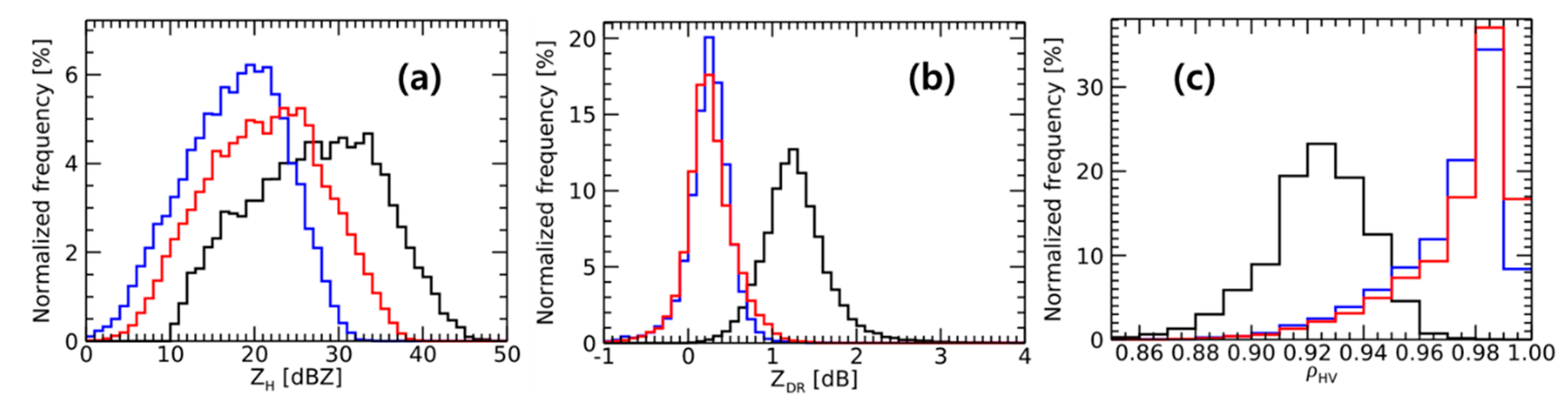
The distributions of polarimetric observations at BBTOP (blue), BBPEAK (black), and BBBOTTOM (red) are shown in Figure 12. ZH Peak mainly ranged between 10 and 45 dBZ, and the average ZH Peak was 27.2 dBZ. The average ZH Top (ZH Bottom) was 21.2 dBZ (17.5 dBZ). The ZH, when the ice particles completely melted, was lower than that when they began to melt. ZDR Peak was distributed between 0.0 and 3.0 dB with an average of 1.28 dB. The average values of ZDR Top and ZDR Bottom were almost similar (0.26 and 0.24 dB). The melting snowflakes were observed to be more oblate than snowflakes and raindrops. ρHV Peak was distributed between the range of 0.86 and 0.97 and was 0.92 on average. The average ρHV Top and ρHV Bottom, which are the threshold values commonly used for BB detection, were identical (0.97).
The results were compared with those obtained under various climatic conditions. In [21] and [26], the authors used X-band radar and [27] used S-band radar to analyze the BB. [21] detected the BB using RHI data from Davos (Swiss Alps), Ardeche (South of France), Iowa (Midwestern USA), and Payerne (Swiss Plateau). [26] constructed the QVPs from a radar located in Born (Germany), while [27] constructed theirs from the WSR-88D radar in the USA. Their BB detection technique was very similar to that of [21] and [26], and [27] applied a technique based on the ρHV. According to [27], QVP allows for more accurate quantification of polarimetric observations than RHI data. Therefore, the results of this study were comparable to those of previous studies. The distribution of ZH Peak, ZDR Peak, and ρHV Peak in Figure 12 were very similar to those in previous study. The average of ZH Peak (27.2 dBZ) was slightly lower than that in the Payerne region (29.0 dBZ), higher than that in the Iowa region (25.46 dBZ), and higher than that obtained by [27] (25.42 dBZ). The average ZDR Peak (1.28 dB) was slightly different from that in the Ardeche region (1.29 dB) and that obtained by [27] (1.13 dB). The ρHV Peak (0.92) was higher than those obtained in Davos and Iowa (0.82), but very consistent with those obtained in the Born region (0.93) and [27] (0.94).
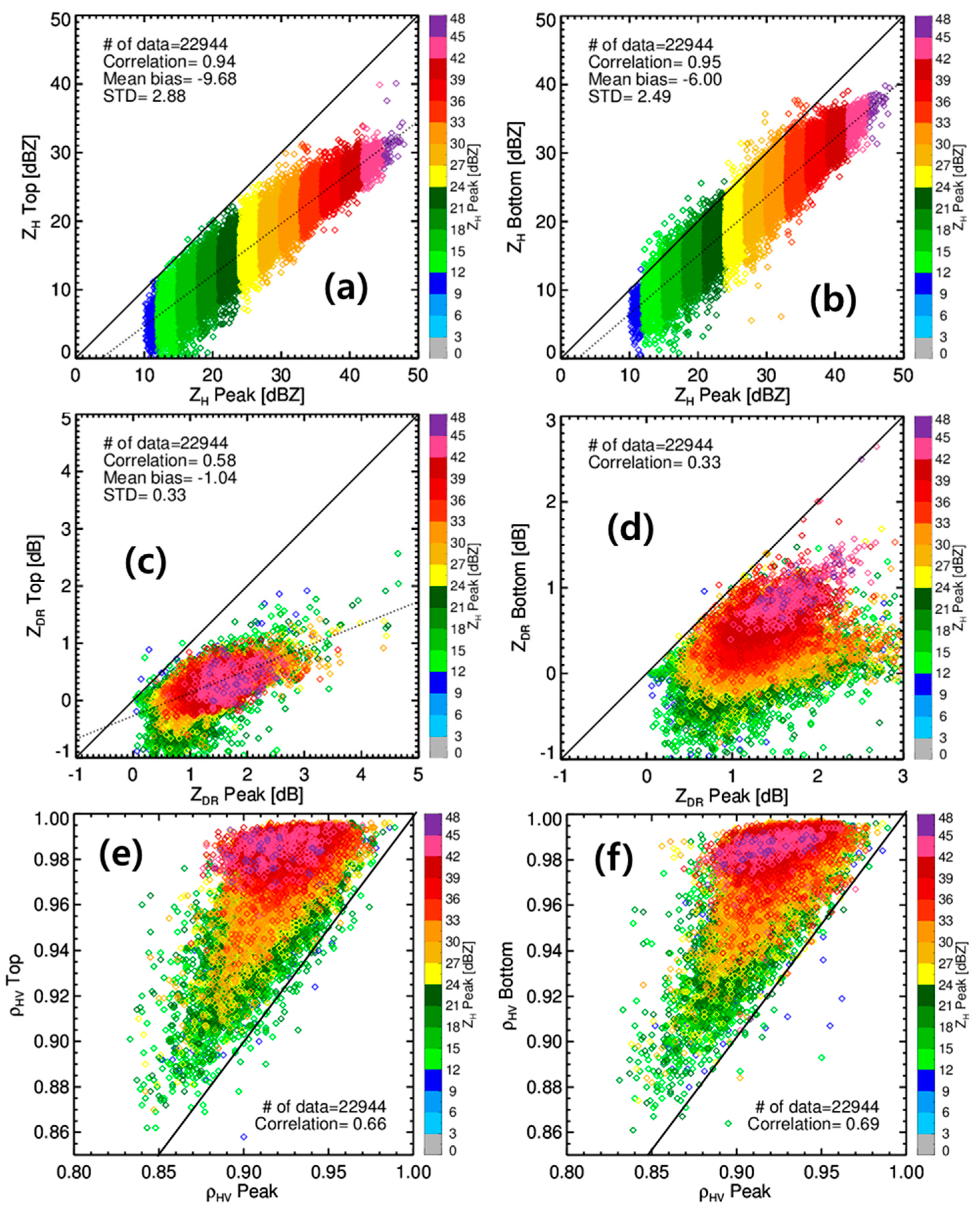
Figure 13 shows scatterplots between ZH Peak and ZH Top/ZH Bottom, ZDR Peak and ZDR Top/ZDR Bottom, and ρHV Peak and ρHV Top/ρHV Bottom. The color of the diamond symbol indicates the ZH Peak. According to [27], a high ZH in the BB represented large snowflakes enlarged via aggregation, and a low ZH mainly represented pristine ice crystals. In addition, a high number of snowflake concentrations increased the number of raindrops after passing the BB. It is apparent from Figure 13a that the mean difference between ZH Top and ZH Peak was 9.68, with a standard deviation of 2.88 dB, and the mean difference between ZH Peak and ZH Bottom was 6.00 dB with a standard deviation of 2.49 dB. Large snowflakes result in an intense BB, which leads to overestimation of rainfall at the surface. ZDR Top and ZDR Peak showed a correlation of 0.58 and a mean difference of −1.04 dB, while ZDR Peak and ZDR Bottom showed a correlation of 0.33. Large snowflakes with high ZH Bottom turn into large raindrops with high ZDR Bottom. Large snowflakes grown by aggregation (represented by high ZH Peak) turn into large raindrops (high ZDR Bottom). In other words, the size of raindrops is related to the growth process of snowflakes above the BB. The difference between ρHV Peak and ρHV Top (between ρHV Peak and ρHV Bottom) increased even more as ZH Peak increased. This results from the inhomogeneity of the hydrometeors’ shape, orientation, and size within the BB since large snowflakes melt more slowly than small snowflakes. In addition, ρHV Peak, ρHV Top, and ρHV Bottom with low ZH Bottom were similar (close to the 1:1 line). This mean that the ρHV shows no distinctive signature for a weak BB.
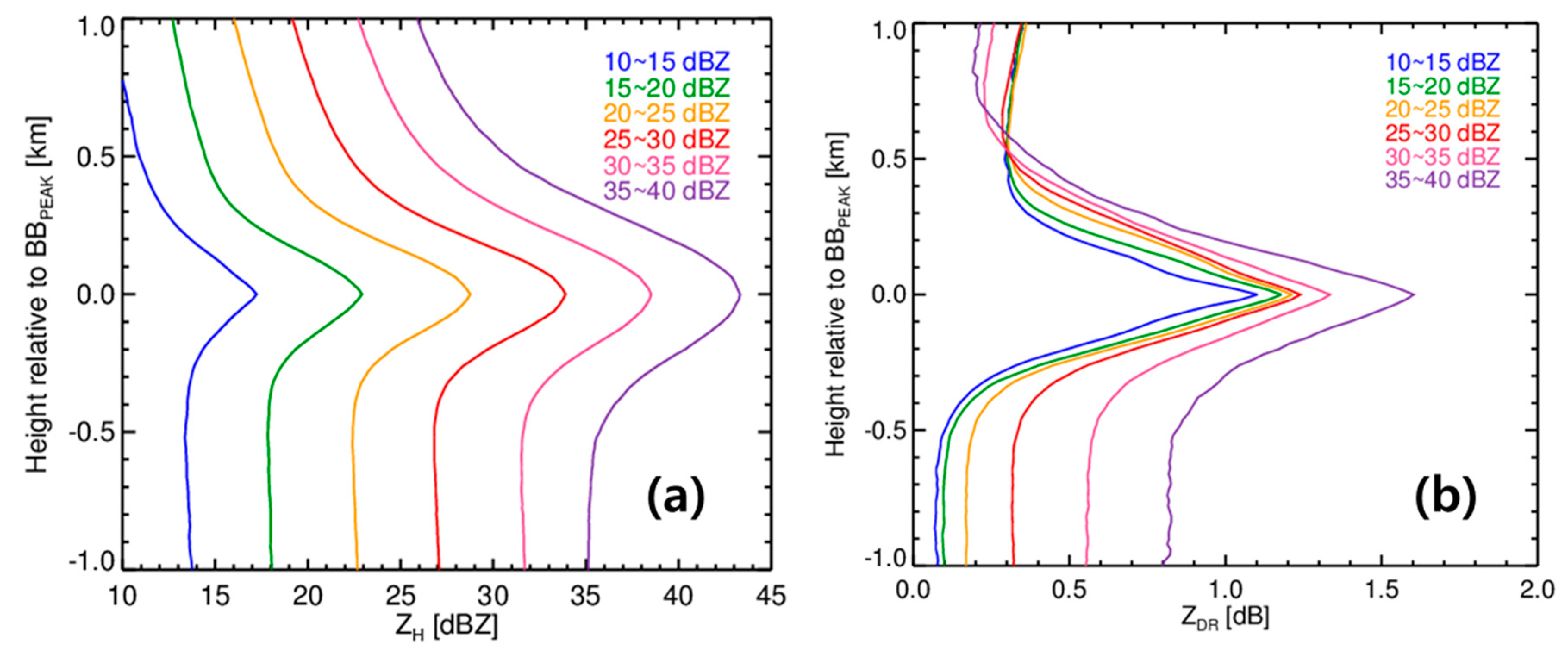
Figure 14 represents the mean profiles of the (a) ZH and (b) ZDR at the ZH Bottom classes with 5 dBZ intervals. H(ZH Peak) and H(ZDR Peak) are reference heights. The maximum ZH and ZDR were located at 0.0 km. The difference in the ZH above the BB and ZH Peak was greater than the difference in the ZH below the BB and ZH Peak. The intensity of the BB depended on ZH Bottom, and the ZH below the BB was almost constant at every class. The size and concentration of snowflakes determined the ZH structure of the BB and the rainfall intensity below the BB. The ZDR decreased above the BB as the snowflake particles smoothen when they start to melt. Large snowflakes (high ZH Bottom class) with a high axis ratio have a low ZDR above the BB. The ZDR within the BB with a high ZH Bottom class was greater than that with a low ZH Bottom class. The ZDR below the BB was larger at the high ZH Bottom class. The shape and orientation of snowflakes determined the ZDR structure of the BB.
4. Conclusions
In this study, we investigated the characteristics of BB in South Korea using QVPs from an operational S-band dual-polarization weather radar network. The BB was automatically identified based on the morphological features from the QVPs of polarimetric observations (ZH, ZDR, and ρHV) using the coordinate rotation technique proposed by [9], and their geometric, thermodynamic, and polarimetric characteristics were statistically examined. The polarimetric observations were corrected before constructing the QVPs for comparable analysis among weather radars in the network. First, the system calibration bias in power-related polarimetric observations (ZH and ZDR) was corrected based on the self-consistency principle between power- and phase-based measurements. Second, the ρHV was biased at low SNR due to noise effects. The precipitation echoes yielded a value that was equal to or greater than 0.98. Unfortunately, an abnormal ρHV was observed in meteorological echoes at a low SNR. The ρHV in low SNR areas was corrected using the SNR. Quality control was performed using the ρHV and SNR to minimize non-meteorological echoes, and then the ZH, ZDR, and ρHV were averaged in the azimuth direction to generate QVPs of polarimetric observations. The ρHV was converted to a new variable to apply the same procedure for the detection of the BB. In this study, the peak of the BB (BBPEAK) was defined as the maximum value by calculating the first gradient. The top and bottom of the BB (BBTOP and BBBOTTOM) were identified via application of the coordinate rotation method developed by [9].
We analyzed the monthly mean height of BBPEAK for all radars in the KMA network. The heights of BBPEAK showed a seasonal variation in all radars (e.g., the highest occurred in the summer). The maximum height of BBPEAK derived from the ZH was 5 km, and the average heights varied within the range from 4.14 to 4.71 km in summer. However, they showed distinct differences depending on the location (e.g., latitude) and the altitude of the radar within the radar network, even in the same season. The heights of BBPEAK differed among the polarimetric observations. The height where melting particles had the most oblate shapes (BBPEAK derived from ZDR) were below that where their size was at maximum (BBPEAK derived from ZH). The inhomogeneity of the hydrometeors was also at maximum (BBPEAK derived from ρHV) below BBPEAK derived from ZH. The height difference of BBPEAK between the ZH and ZDR, and that between ZH and ρHV increased with increasing ZH Bottom. The difference in heights of ZH Peak and ρHV Peak was similar to that in previous studies under various climatic conditions.
The relative position (r) of BBPEAK (defined as the height difference between BBPEAK and BBBOTTOM to the BB thickness) and the BB thickness were calculated to analyze the geometric characteristics of the BB. The difference in heights between BBPEAK and BBTOP (BBBOTTOM) was 430–460 m (350 m). The BB thickness represented by the ZH and ZDR tended to increase with increasing ZH Bottom. The r was less than 0.5 for all variables, and BBPEAK was close to BBBOTTOM. The r for the QVP of ZDR was close to 0.5 if ZH Bottom was low, and the r decreased to 0.4 if ZH Bottom was high. We confirmed from these results that the structure of the BB was asymmetrical and depended on ZH Bottom.
The thermodynamic characteristics were analyzed by comparing the BB heights and zero isothermal layers of dry-bulb, dew point, and wet-bulb temperatures. The zero-isotherm layer of the dry-bulb temperature was located between BBTOP and BBBOTTOM and was closer to the zero-isotherm layer of the welt-bulb temperature. BBTOP was located above the zero temperature (−1.96 to −1.03 °C), and BBPEAK was located below the zero temperature (0.73 to 1.16 °C).
The microphysical process associated with the BB was investigated by analyzing the polarimetric observations in the BB. The polarimetric observations at BBPEAK were compared with those in previous studies. The distribution of polarimetric observations was very similar, although previous studies utilized different frequencies, radar scan strategies, and BB detection techniques. The ZH at BBPEAK averaged 27.2 dB, with a difference of 9.68 (6.00) dB from that at BBTOP (BBBOTTOM). The ZDR at BBPEAK was 1.28 dB, which was higher than the ZDR at BBTOP (0.26 dB) and BBBOTTOM (0.24 dB). The ρHV at BBPEAK was 0.92, whereas that at BBTOP and BBBOTTOM was 0.97, which is the threshold traditionally used for the detection of the BB. The relation between polarimetric observations at BBPEAK, BBTOP, and BBBOTTOM represented the microphysical properties of the BB. The ZH at BBPEAK, BBTOP, and BBBOTTOM was highly correlated. This means that large snowflakes turn into large raindrops. It was also confirmed that the ZDR at BBBOTTOM and BBPEAK showed a positive relation with a high ZH at BBPEAK. The mean profiles of ZH and ZDR also depended on the size and concentration of the snowflakes above the BB.
In conclusion, the characteristics of BB from the QVPs of polarimetric observations were investigated in this study. The three-dimensional detection of BB and its intensity correction remain a challenge. Especially, this is more difficult in the cold season because the vertical structure of BB cannot be fully identified when they occur near the surface. The polarimetric observations above, within, and below the BB revealed in this study provide the characteristics of the BB related to microphysical processes. The results contribute by promoting an understanding of polarimetric signatures within BB and ultimately improve the performance of BB correction techniques. Furthermore, the NWP can represent the microphysical processes within BB, and the zero isothermal layer identified from radar observations can be used for NWP data assimilation.
Author Contributions
This work was possible through significant contributions from all authors. Conceptualization, S.-H.J., J.-E.L. and S.K.; methodology, S.-H.J., J.-E.L. and S.K.; software, J.-E.L., S.-H.J. and S.K.; formal analysis, J.-E.L.; investigation, J.-E.L.; writing—original draft preparation, S.-H.J. and J.-E.L.; writing—review and editing, S.-H.J. and J.-E.L.; visualization, J.-E.L.; supervision, S.-H.J.; funding acquisition, S.-H.J. All authors have read and agreed to the published version of the manuscript.
Funding
This research is supported by “Development and application of cross governmental dual-pol radar harmonization (WRC-2013-A-1)” project of the Weather Radar Center, Korea Meteorological Administration.
Conflicts of Interest
The authors declare no conflict of interest.
References
- Fabry, F.; Zawadzki, I. Long-term radar operations of the melting layer of precipitation and their interpretation. J. Atmos. Sci. 1995, 52, 838–851. [Google Scholar] [CrossRef]
- Szyrmer, W.; Zawadzki, I. Modeling of the melting layer. Part I: Dynamics and microphysics. J. Atmos. Sci. 1999, 56, 3573–3592. [Google Scholar]
- Bellon, A.; Lee, G.W.; Zawadzki, I. Error statistics of VPR corrections in stratiform precipitation. J. Appl. Meteor. 2005, 44, 998–1015. [Google Scholar] [CrossRef] [Green Version]
- Germann, U.; Joss, J. Mesobeta profiles to extrapolate radar precipitation measurements above the Alps to the ground level. J. Appl. Meteor. 2002, 41, 542–557. [Google Scholar] [CrossRef]
- Vignal, B.; Krajewski, W. Large-sample evaluation of two methods to correct range-dependent error for WSR-88D rainfall estimates. J. Hydrometeor. 2001, 2, 490–504. [Google Scholar] [CrossRef]
- Tilford, K.A.; Cluckie, I.D.; Griffith, R.J.; Lane, A. Vertical reflectivity characteristics and bright band correction. In Radar Hydrology for Real Time Flood Forecasting, Proceedings of an Advanced Study Course; Griffith, R.J., Cluckie, I.D., Austin, G.L., Han, D., Eds.; EUR-OP: Luxembourg, 2001; pp. 47–65. [Google Scholar]
- Gray, W.R.; Uddstrom, M.J.; Larsen, H.R. Radar surface rainfall estimates using a typical shape function approach to correct for the variations in the vertical profile of reflectivity. Int. J. Remote Sens. 2002, 23, 2489–2504. [Google Scholar] [CrossRef]
- Gourley, J.J.; Calvert, C.M. Automated detection of the bright band using WSR-88D data. Weather Forecast. 2003, 18, 585–598. [Google Scholar] [CrossRef]
- Rico-Ramirez, M.A.; Cluckie, I.D. Bright-band detection from radar vertical reflectivity profiles. Int. J. Remote Sens. 2007, 28, 4013–4025. [Google Scholar] [CrossRef]
- Zhang, J.; Langston, C.; Howard, K. Bright band identification based on vertical profiles of reflectivity from the WSR-88D. J. Atmos. Ocean. Technol. 2008, 25, 1859–1872. [Google Scholar] [CrossRef]
- Klaassen, W. Radar observations and simulations of the melting layer of precipitation. J. Atmos. Sci. 1988, 45, 3741–3753. [Google Scholar] [CrossRef]
- White, A.B.; Gottas, D.J.; Strem, E.T.; Ralph, F.M.; Neiman, P.J. An automated bright band height detection algorithm for use with Doppler radar spectral moments. J. Atmos. Ocean. Technol. 2002, 19, 687–697. [Google Scholar] [CrossRef] [Green Version]
- Ryzhkov, A.; Zrnić, D. Discrimination between rain and snow with a polarimetric radar. J. Appl. Meteor. 1998, 37, 1228–1440. [Google Scholar] [CrossRef]
- Brandes, E.; Ikeda, K. Freezing-level estimation with polarimetric radar. J. Appl. Meteorol. 2004, 43, 1541–1553. [Google Scholar] [CrossRef]
- Tabary, P.; Henaff, A.; Vulpiani, G.; Parent-du-Chatelet, J.; Gourley, J. Melting layer characterization and identification with a C-band dual-polarization radar: A long term analysis. In Proceedings of the Fourth European Conference on Radar in Meteorology and Hydrology (ERAD 2006), Barcelona, Spain, 18–22 September 2006; Servei Meteorològic de Catalunya: Barcelona, Spain, 2006; pp. 17–20. [Google Scholar]
- Giangrande, S.E.; Krause, J.M.; Ryzhkov, A.V. Automated designation of the melting layer with a polarimetric prototype of the WSR-88D radar. J. Appl. Meteor. Climatol. 2008, 47, 1354–1364. [Google Scholar] [CrossRef]
- Islam, T.; Rico-Ramirez, M.A.; Han, D.W.; Bray, M.; Srivastava, P.K. Fuzzy logic based melting layer recognition from 3 GHz dual polarization radar: Appraisal with NWP model and radio sounding observations. Theor. Appl. Climatol. 2013, 112, 317–338. [Google Scholar] [CrossRef]
- Boodoo, S.; Hudak, D.; Donaldson, N.; Leduc, M. Application of dual-polarization radar melting-layer detection algorithm. J. Appl. Meteorol. Climatol. 2010, 49, 1779–1793. [Google Scholar] [CrossRef]
- Illingworth, A.; Thompson, R. Radar bright band correction using the linear depolarisation ratio. In Proceedings of the Eighth International Symposium on Weather Radar and Hydrology, Exeter, UK, 18–21 April 2011; IAHS Publication: Wallingford, UK, 2011; Volume 351, pp. 64–68. [Google Scholar]
- Zawadzki, I.; Szyrmer, W.; Bell, C.; Fabry, F. Modeling of the melting layer. Part III: The density effect. J. Atmos. Sci. 2005, 62, 3705–3723. [Google Scholar] [CrossRef]
- Wolfensberger, D.; Scipion, D.; Berne, A. Detection and characterization of the melting layer based on polarimetric radar scans. Q. J. R. Meteorol. Soc. 2015, 142, 108–124. [Google Scholar] [CrossRef]
- Kumjian, M.R.; Ryzhkov, A.V.; Reeves, H.D.; Schuur, T.J. A dual polarization radar signature of hydrometeor refreezing in winter storms. J. Appl. Meteor. Climatol. 2013, 52, 2549–2566. [Google Scholar] [CrossRef]
- Kumjian, M.R.; Lombardo, K.A. Insights into the evolving microphysical and kinematic structure of northeastern U.S. winter storms from dual-polarization Dopper radar. Mon. Weather Rev. 2017, 145, 1033–1061. [Google Scholar] [CrossRef]
- Ryzhkov, A.V.; Zhang, P.; Reeves, H.D.; Kumjian, M.R.; Tschallener, T.; Trömel, S.; Simmer, C. Quasi-vertical profiles—A new way to look at polarimetric radar data. J. Atmos. Ocean. Technol. 2016, 33, 551–562. [Google Scholar] [CrossRef]
- Kim, H.L.; Jung, S.H.; Jang, K.I. Estimating rain microphysical characteristics using S-band dual-polarization radar in South Korea. J. Atmos. Ocean. Technol. 2020, 33, 551–562. [Google Scholar] [CrossRef] [Green Version]
- Trömel, S.; Ryzhkov, A.V.; Hickman, B.; Muhlbauer, K.; Simmer, C. Polarimetric radar variables in the layers of melting and dendritic growth at X band—Implications for a nowcasting strategy in stratiform rain. J. Appl. Meteorol. Climatol. 2019, 58, 2497–2522. [Google Scholar] [CrossRef]
- Griffin, E.M.; Schuur, T.J.; Ryzhkov, A.V. A polarization radar analysis of ice microphysical processes in melting layers of winter storms using S-band qusai-vertical profiles. J. Appl. Meteorol. Climatol. 2020, 59, 751–767. [Google Scholar] [CrossRef]
- Lee, J.-E.; Jung, S.-H.; Kim, J.-S.; Jang, K. Sensitivity analysis of polarimetric observations by two different pulse lengths of dual-polarization weather radar. Atmosphere 2019, 29, 192–211, (In Korean with English abstract). [Google Scholar]
- Kim, M.; Lee, K.; Lee, Y.H. Visibility Data Assimilation and Prediction Using an Observation Network in South Korea. Pure Appl. Geophys. 2019, 177, 1125–1141. [Google Scholar] [CrossRef]
- Lee, G.W.; Zawadzki, I. Radar calibration by gate, disdrometer, and polarimetry: Theoretical limit caused by the variability of drop size distribution and application to fast scanning operational radar data. J. Hydrol. 2006, 328, 83–97. [Google Scholar] [CrossRef]
- Kwon, S.; Lee, G.W.; Kim, G. Rainfall estimation from an operational S-band dual-polarization radar: Effect of radar calibration. J. Meteor. Soc. Jpn. 2015, 93, 65–79. [Google Scholar] [CrossRef] [Green Version]
- Ryzhkov, A.; Zrnić, D. Radar Polarimetry for Weather Observations; Springer: Cham, Switzerland, 2019; p. 486. [Google Scholar]
- Durden, S.L.; Kitiyakara, A.; Eastwood, I.; Tanner, A.B.; Haddad, Z.S.; Li, F.K.; Wilson, W.J. ARMAR observations of the melting layer during TOGA COARE. IEEE Trans. Geosci. Remote Sens. 1997, 35, 1453–1456. [Google Scholar] [CrossRef]
- Khanal, A.K.; Delrieu, G.; Cazenave, F.; Boudevillain, B. Radar Remote Sensing of Precipitation in High Mountains: Detection and Characterization of Melting layer in the Grenoble Valley, French Alps. Atmosphere 2019, 10, 784. [Google Scholar] [CrossRef] [Green Version]
Figure 1.
Deployment of the Korea Meteorological Administration (KMA) S-band dual-polarization weather radar network. The 10 circles indicate the 240 km radius coverage of the radar.
Figure 1.
Deployment of the Korea Meteorological Administration (KMA) S-band dual-polarization weather radar network. The 10 circles indicate the 240 km radius coverage of the radar.

Figure 2.
Quasi-vertical profile (QVP) of the ZH and the parameters defined for rotating coordinates. (a) Original coordinate; (b) New coordinate after 90° rotation; (c) Final coordinate after degree rotation. The thin lines indicate the top, peak, and bottom of the bright band (BB) derived from the QVP of the ZH.

Figure 3.
Time series of quasi-vertical profiles (QVPs) of the (a) ZH, (c) ZDR, and (e) ρHV and the height of the top (blue), peak (black), and bottom (red) of the BB from the (b) ZH, (d) ZDR, and (f) ρHV at elevation angles of 15.0° of the BRI radar from 0000 KST of 6 September 2019 to 1800 KST of 7 September 2019. The solid and dashed lines indicate the heights where T is 0 °C and Tw is 0 °C, respectively.

Figure 4.
Monthly variation in mean height for BBPEAK identified using the ZH from March to November from the individual radar across the KMA weather radar network. The blue to red color indicates radar located from higher to lower latitudes.
Figure 4.
Monthly variation in mean height for BBPEAK identified using the ZH from March to November from the individual radar across the KMA weather radar network. The blue to red color indicates radar located from higher to lower latitudes.

Figure 5.
Two-dimensional frequency distribution (a) between H(ZDR Peak) and H(ZH Peak) and (b) between H(ρHV Peak) and H(ZH Peak).
Figure 5.
Two-dimensional frequency distribution (a) between H(ZDR Peak) and H(ZH Peak) and (b) between H(ρHV Peak) and H(ZH Peak).

Figure 6.
Box plots of the mean differences between H(ZH Peak) and H(ZDR Peak) (a), and between H(ZH Peak) and H(ρHV Peak) (b) as a function of ZH Bottom. The black (red) dotted line indicates no difference (the mean height difference).
Figure 6.
Box plots of the mean differences between H(ZH Peak) and H(ZDR Peak) (a), and between H(ZH Peak) and H(ρHV Peak) (b) as a function of ZH Bottom. The black (red) dotted line indicates no difference (the mean height difference).

Figure 7.
Two-dimensional frequency distributions. (a) Between H(ZH Top) and H(ZH Peak); (b) Between H(ZDR Top) and H(ZDR Peak); (c) Between H(ρHV Top) and H(ρHV Peak); (d) Between H(ZH Bottom) and H(ZH Peak); (e) Between H(ZDR Bottom) and H(ZDR Peak); and (f) between H(ρHV Bottom) and H(ρHV Peak).
Figure 7.
Two-dimensional frequency distributions. (a) Between H(ZH Top) and H(ZH Peak); (b) Between H(ZDR Top) and H(ZDR Peak); (c) Between H(ρHV Top) and H(ρHV Peak); (d) Between H(ZH Bottom) and H(ZH Peak); (e) Between H(ZDR Bottom) and H(ZDR Peak); and (f) between H(ρHV Bottom) and H(ρHV Peak).

Figure 8.
Box plots of the thickness of the BB (left) and relative position of BBPEAK (right) as a function of ZH BBBOTTOM. The dashed line indicates the symmetric structure of the BB.
Figure 8.
Box plots of the thickness of the BB (left) and relative position of BBPEAK (right) as a function of ZH BBBOTTOM. The dashed line indicates the symmetric structure of the BB.

Figure 9.
Two-dimensional frequency distributions between (a) H(ZH Top) and H(T = 0 °C) and between (b) H(ZH Top) and H(Tw = 0 °C).
Figure 9.
Two-dimensional frequency distributions between (a) H(ZH Top) and H(T = 0 °C) and between (b) H(ZH Top) and H(Tw = 0 °C).

Figure 10.
Two-dimensional frequency distributions between (a) H(ZH Peak) and H(T = 0 °C) and between (b) H(ZH Peak) and H(Tw = 0 °C).
Figure 10.
Two-dimensional frequency distributions between (a) H(ZH Peak) and H(T = 0 °C) and between (b) H(ZH Peak) and H(Tw = 0 °C).

Figure 11.
Normalized frequency distribution of (a,d,g) T, (b,e,h) Td, and (c,f,i) Tw at top (blue), peak (black), and bottom (red) of bright band from QVPs of (a–c) ZH, (d–f) ZDR, and (g–i) ρHV.
Figure 11.
Normalized frequency distribution of (a,d,g) T, (b,e,h) Td, and (c,f,i) Tw at top (blue), peak (black), and bottom (red) of bright band from QVPs of (a–c) ZH, (d–f) ZDR, and (g–i) ρHV.

Figure 12.
Normalized frequency distribution of (a) ZH, (b) ZDR, and (c) ρHV at top (blue), peak (black), and bottom (red) of the BB.
Figure 12.
Normalized frequency distribution of (a) ZH, (b) ZDR, and (c) ρHV at top (blue), peak (black), and bottom (red) of the BB.

Figure 13.
Scatter plots of (a) ZH Top and ZH Peak, (b) ZDR Top and ZDR Peak, (c) ρHV Top and ρHV Peak, (d) ZH Bottom and ZH Peak, (e) ZDR Bottom and ZDR Peak, and (f) ρHV Bottom and ρHV Peak. Colors indicate the ZH Peak with 3 dBZ intervals.
Figure 13.
Scatter plots of (a) ZH Top and ZH Peak, (b) ZDR Top and ZDR Peak, (c) ρHV Top and ρHV Peak, (d) ZH Bottom and ZH Peak, (e) ZDR Bottom and ZDR Peak, and (f) ρHV Bottom and ρHV Peak. Colors indicate the ZH Peak with 3 dBZ intervals.

Figure 14.
Mean profile of the (a) ZH and (b) ZDR with respect to the height relative to BBPEAK at the ZH Bottom classes with 5 dBZ intervals.
Figure 14.
Mean profile of the (a) ZH and (b) ZDR with respect to the height relative to BBPEAK at the ZH Bottom classes with 5 dBZ intervals.


Table 1.
Scan strategy of KMA operational S-band dual-polarization radars.
| Radar | Elevation Angle (°) | ||||||||
|---|---|---|---|---|---|---|---|---|---|
| GDK | −0.40 | 0.01 | 0.31 | 0.80 | 1.41 | 2.50 | 4.20 | 7.11 | 15.01 |
| BRI | 0.10 | 0.42 | 0.81 | 1.41 | 2.20 | 3.41 | 5.10 | 7.61 | 15.01 |
| KWK | −0.19 | 0.00 | 0.30 | 0.81 | 1.50 | 2.60 | 4.40 | 7.30 | 15.01 |
| MYN | −0.80 | −0.39 | 0.01 | 0.41 | 0.91 | 1.91 | 3.60 | 7.00 | 15.01 |
| KSN | 0.00 | 0.30 | 0.70 | 1.30 | 2.10 | 3.21 | 5.00 | 7.61 | 15.01 |
| PSN | −0.09 | 0.20 | 0.60 | 1.10 | 1.81 | 3.00 | 4.71 | 7.40 | 15.01 |
| JNI | −0.09 | 0.20 | 0.60 | 1.10 | 1.81 | 3.00 | 4.71 | 7.42 | 15.02 |
| SSP | 0.20 | 0.50 | 1.01 | 1.60 | 2.41 | 3.50 | 5.20 | 7.60 | 15.00 |
| GSN | 0.20 | 0.50 | 1.01 | 1.60 | 2.41 | 3.50 | 5.20 | 7.60 | 15.01 |
Table 2.
Definitions of feature parameters for characterizing the BB.
| Feature Parameters | Definition |
|---|---|
| H(ZH Top) | Height of identified by QVP of ZH |
| H(ZH Peak) | Height of identified by QVP of ZH |
| H(ZH Bottom) | Height of identified by QVP of ZH |
| H(ZDR Top) | Height of identified by QVP of ZDR |
| H(ZDR Peak) | Height of identified by QVP of ZDR |
| H(ZDR Bottom) | Height of identified by QVP of ZDR |
| H(ρHV Top) | Height of identified by QVP of ρHV |
| H(ρHV Peak) | Height of identified by QVP of ρHV |
| H(ρHV Bottom) | Height of identified by QVP of ρHV |
| H( = 0 °C) | Height where is 0° |
| H( = 0 °C) | Height where is 0° |
| H( = 0 °C) | Height where is 0° |
| ZH Top | ZH value at H(ZH Top) |
| ZH Peak | ZH value at H(ZH Peak) (i.e., Maximum ZH in BB) |
| ZH Bottom | ZH value at H(ZH Bottom) |
| ZDR Top | ZDR value at H(ZDR Top) |
| ZDR Peak | ZDR value at H(ZDR Peak) (i.e., Maximum ZDR in BB) |
| ZDR Bottom | ZDR value at H(ZDR Bottom) |
| ρHV Top | ρHV value at H(ρHV Top) |
| ρHV Peak | ρHV value at H(ρHV Peak) (i.e., Minimum ρHV in BB) |
| ρHV Bottom | ρHV value at H(ρHV Bottom) |
Table 3.
Monthly mean height of BBPEAK at each radar sorted in ascending order according to latitude.
Table 3.
Monthly mean height of BBPEAK at each radar sorted in ascending order according to latitude.
| Radar | MAR | APR | MAY | JUN | JUL | AUG | SEP | OCT | NOV |
|---|---|---|---|---|---|---|---|---|---|
| GDK | 2.58 | 1.79 | - | 3.54 | 4.56 | 4.83 | 4.35 | 3.45 | 2.44 |
| BRI | 1.96 | 1.85 | 4.20 | 3.57 | 4.37 | 4.15 | 4.36 | 2.59 | 1.80 |
| KWK | 2.53 | 2.24 | - | 4.12 | 4.46 | 4.74 | 4.29 | 3.71 | 2.25 |
| MYN | 3.10 | 2.99 | 3.21 | 4.54 | 4.75 | 4.77 | 4.29 | 3.35 | 3.14 |
| KSN | 2.17 | 3.33 | 3.35 | 4.55 | 4.86 | 5.00 | 4.44 | 4.09 | 2.87 |
| PSN | 2.28 | 2.81 | 3.58 | 4.36 | 4.81 | 4.85 | 4.55 | 3.70 | - |
| JNI | 2.73 | 2.94 | 3.94 | 4.39 | 4.58 | 4.68 | 4.51 | 4.25 | 3.15 |
| SSP | 1.83 | 3.59 | 4.04 | 4.11 | 4.81 | 4.70 | 4.52 | 3.92 | 2.68 |
| GSN | 1.93 | 3.20 | 4.09 | 4.06 | 4.84 | 4.66 | 4.61 | 4.14 | 2.68 |
| Mean | 2.35 | 2.75 | 3.77 | 4.14 | 4.67 | 4.71 | 4.43 | 3.69 | 2.62 |
Table 4.
Mean and standard deviation (STD) of temperature (T), dew point temperature (Td), and wet-bulb temperature (Tw) at the top, peak, and bottom of the BB.
Table 4.
Mean and standard deviation (STD) of temperature (T), dew point temperature (Td), and wet-bulb temperature (Tw) at the top, peak, and bottom of the BB.
| at H(ZH Bottom/Peak/Top) | at H(ZH Bottom/Peak/Top) | at H(ZH Bottom/Peak/Top) | |||||||
| MEAN | 2.41 | 0.73 | −1.33 | 0.64 | −0.89 | −2.90 | 1.53 | −0.04 | −2.03 |
| STD | 1.55 | 1.32 | 1.39 | 3.34 | 3.24 | 3.36 | 1.71 | 1.52 | 1.58 |
| at H(ZDR Bottom/Peak/Top) | at H(ZDR Bottom/Peak/Top) | at H(ZDR Bottom/Peak/Top) | |||||||
| MEAN | 2.71 | 1.04 | −1.96 | 0.92 | −0.61 | −2.63 | 1.82 | 0.25 | −1.76 |
| STD | 1.63 | 1.47 | 1.42 | 3.39 | 3.31 | 3.38 | 1.79 | 1.65 | 1.60 |
| at H(ρHV Bottom/Peak/Top) | at H(ρHV Bottom/Peak/Top) | at H(ρHV Bottom/Peak/Top) | |||||||
| MEAN | 2.84 | 1.16 | −1.03 | 1.03 | −0.49 | −2.60 | 1.93 | 0.37 | −1.73 |
| STD | 1.65 | 1.44 | 1.51 | 3.39 | 3.28 | 3.40 | 1.79 | 1.60 | 1.69 |
Publisher’s Note: MDPI stays neutral with regard to jurisdictional claims in published maps and institutional affiliations. |
© 2020 by the authors. Licensee MDPI, Basel, Switzerland. This article is an open access article distributed under the terms and conditions of the Creative Commons Attribution (CC BY) license (http://creativecommons.org/licenses/by/4.0/).
Share and Cite
MDPI and ACS Style
Lee, J.-E.; Jung, S.-H.; Kwon, S. Characteristics of the Bright Band Based on Quasi-Vertical Profiles of Polarimetric Observations from an S-Band Weather Radar Network. Remote Sens. 2020, 12, 4061. https://doi.org/10.3390/rs12244061
AMA Style
Lee J-E, Jung S-H, Kwon S. Characteristics of the Bright Band Based on Quasi-Vertical Profiles of Polarimetric Observations from an S-Band Weather Radar Network. Remote Sensing. 2020; 12(24):4061. https://doi.org/10.3390/rs12244061
Chicago/Turabian StyleLee, Jeong-Eun, Sung-Hwa Jung, and Soohyun Kwon. 2020. "Characteristics of the Bright Band Based on Quasi-Vertical Profiles of Polarimetric Observations from an S-Band Weather Radar Network" Remote Sensing 12, no. 24: 4061. https://doi.org/10.3390/rs12244061
Note that from the first issue of 2016, this journal uses article numbers instead of page numbers. See further details here.