Application of Spectral Mixture Analysis to Vessel Monitoring Using Airborne Hyperspectral Data
by
 , , and
Jae-Jin Park
1, 
Tae-Sung Kim
2,
Kyung-Ae Park
3,*,
Sangwoo Oh
2,
Moonjin Lee
2 and
Pierre-Yves Foucher
4 1
Department of Science Education, Seoul National University, Seoul 08826, Korea
2
Maritime Safety and Environmental Research Division, Korea Research Institute of Ships and Ocean Engineering, Daejeon 38103, Korea
3
Department of Earth Science Education/Research Institute of Oceanography, Seoul National University, Seoul 08826, Korea
4
Theoretical and Applied Optics Department, Office National d’Etudes et Recherches Aérospatiales, F-31055 Toulouse, France
*
Author to whom correspondence should be addressed.
Remote Sens. 2020, 12(18), 2968; https://doi.org/10.3390/rs12182968
Submission received: 27 July 2020
/
Revised: 7 September 2020
/
Accepted: 10 September 2020
/
Published: 11 September 2020
(This article belongs to the Special Issue Optical Oceanographic Observation)
Abstract
:As marine transportation has increased in coastal regions, maritime accidents associated with vessels have steadily increased. Remotely sensed satellite or airborne images can aid rapid vessel monitoring over wide areas at high resolutions. In this study, airborne hyperspectral experiments were performed to detect marine vessels mainly including fishing boat and yacht by applying pixel-based mixture techniques and to estimate the size of the vessels through an objective ellipse fitting method. Various spectral libraries of marine objects and seawaters were constructed through in-situ experiments for spectral analysis of the internal structures of vessels. The hyperspectral images were dimensionally reduced through principal component analysis. Several hyperspectral mixture algorithms, such as N-FINDR, pixel purity index (PPI), independent component analysis (ICA), and vertex component analysis (VCA), were used for the detection of vessels. The N-FINDR and VCA techniques presented a total of 14 vessels, the ICA technique detected seven vessels, and the PPI technique detected two vessels. The pixel-based probability of detection (POD) and false alarm ratio (FAR) for all 14 vessels were 96.40% and 4.30%, respectively. The sizes of the vessels were estimated by extracting the boundaries of the vessels through a two-dimensional gradient and applying the ellipse fitting method. Compared with the digital mapping camera (DMC) images with resolutions of 0.10 m, the root-mean-square errors of the length and width of the vessels were approximately 1.19 m and 0.81 m, respectively. The application of spectral mixing methods provided a high probability of detecting the objects, as well as the overall structures of the decks of the vessels.
1. Introduction
Coastal regions are characterized by complex coastal sea waters, with waves, tides, tidal flats, and diverse geographical features such as sand shores, bays, and deltas. These regions provide important ecological, chemical, and geologically unique environments, making them suitable for human habitation and production activities. Consequently, 23% of the world’s population lives in coastal areas, and two-thirds of large cities with populations of more than 10 million are located offshore [1,2,3]. Coastal regions play a very important role in several sea-traffic routes. The Korean Peninsula is surrounded by ocean on three sides, and the ports and industrial areas are concentrated along complex coastlines. Recently, shipping maritime traffic has been increasing, and more vessels operating around the ports have led to an increasing number of maritime traffic accidents such as vessel collisions, stranding, and explosions. According to the Ministry of Ocean and Fisheries of Korea, the number of vessel accidents has been increased with a rate of approximately 70% over the last six years (https://www.kmst.go.kr). Thus, it is necessary to monitor vessels in real time to prepare for marine accidents and to effectively manage coastal regions. In the event of a marine accident, a rapid search of vessels is needed. Searching for vessels can be conducted by boarding vessels, using helicopters, or using radars around the point of the accident. Most accidents occur under poor weather conditions when winds are strong or waves are high. Such conditions have prevented the rapid detection of vessels. In light of this, high resolution remote sensing methods using satellites or aircraft can contribute to efficient monitoring over a wide area [4].
Conventional vessel detection studies using satellites have been conducted mainly using optical and synthetic aperture radar (SAR) sensors. An optical remote sensing vessel detection study began in 1978 using the threshold method on Landsat-2 Multispectral Scanner (MSS) imaging [5]. Since 2000, the launch of IKONOS and Satellite Pour l’Observation de la Terre (SPOT)-5 high-resolution optical satellites with resolutions of approximately 5 m has made it possible to distinguish not only vessels, but their shapes and textures. With the development of image processing techniques, various methods such as the canny edge, Fourier transform, Bayesian method, and random forest methods have been applied [6,7,8]. Recently, artificial intelligence has been applied to optical satellite images, and a machine learning vessel detection study using support vector machine (SVM) has been conducted. Deep learning research has progressed rapidly, enabling the detection and classification of vessels in images by modeling patterns in data into complex multi-layer networks. During extreme atmospheric conditions, high-resolution SAR images have been used to detect vessels [9,10,11,12,13,14]. In SAR images, the vessel pixels are normally bright, with a larger normalized radar cross section (NRCS) value, which clearly discriminates from the dark pixels. To classify the vessel from the surrounding background field, several algorithms have been developed and utilized for SAR images. The constant false alarm rate (CFAR) algorithm is one of the most well-known and widely used methods to distinguish the vessel pixels from the SAR data by selecting the most appropriate probability density function for the background field surrounding the vessel [15,16,17,18,19,20,21,22]. However, SAR images have some disadvantages in terms of limited observation frequency.
Multispectral sensors acquire limited spectral information at limited channels of ten or fewer spectral bands. In contrast, a hyperspectral sensor has the advantage of extracting more detailed spectral characteristics of objects by hundreds of narrow and continuous channels. Hyperspectral observations have been used not only in ocean regions but also in other atmospheric and land applications such as terrestrial classification, atmospheric correction, mineral mapping, and ocean water quality analysis [23,24,25,26,27,28,29,30,31,32,33,34,35]. Because the hyperspectral sensor can acquire a large amount of spectral information of ground objects, it can be sufficiently utilized in the field of remote vessel detection. However, few studies have attempted to detect vessels partly because of the relatively low spatial resolution of hyperspectral satellite images with frequent spectral noise [4,36]. In contrast to satellite data, airborne measurements can provide high spatial resolution image data. A previous study focused on the detection of floating objects such as non-vessels and surfboards with diverse colors using the vertex component analysis (VCA) method as a representative classification technique [37]. A hyperspectral method for ship detection has been validated by conducting a cruise campaign as well as airborne measurements using an airborne visible/infrared imaging spectrometer (AVIRIS) hyperspectral sensor [38]. Further study should enhance the capability of the detection methods by implementing the construction of an in-situ spectral library of additional floating objects and vessels.
Considering such aspects, in this study, we conducted an airborne experiment with a hyperspectral camera and conducted a ground experiment to obtain the spectra of the objects. The four objectives of this study were to: (1) perform a hyperspectral airborne experiment to obtain high-resolution images in the coastal region containing a large number of vessels, (2) construct a maritime library by measuring the spectrum of various vessel structures and seawater, (3) detect vessels and various objects on the decks and classify them by using various spectral mixture techniques, and (4) to apply the ellipse fitting method to the pixels corresponding to the vessel to estimate the size of the vessel.
2. Data and Methods
2.1. Airborne Hyperspectral Measurements
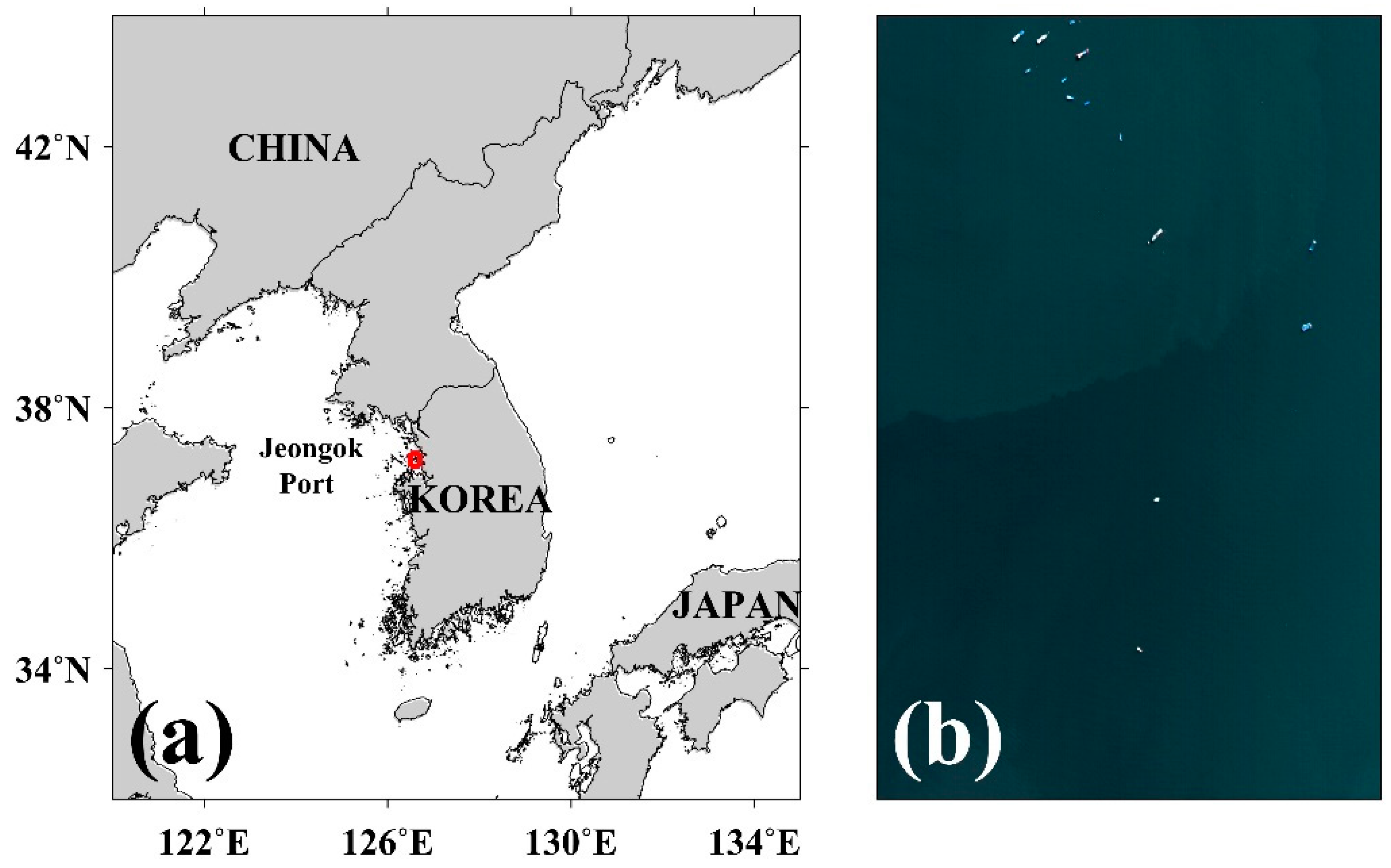
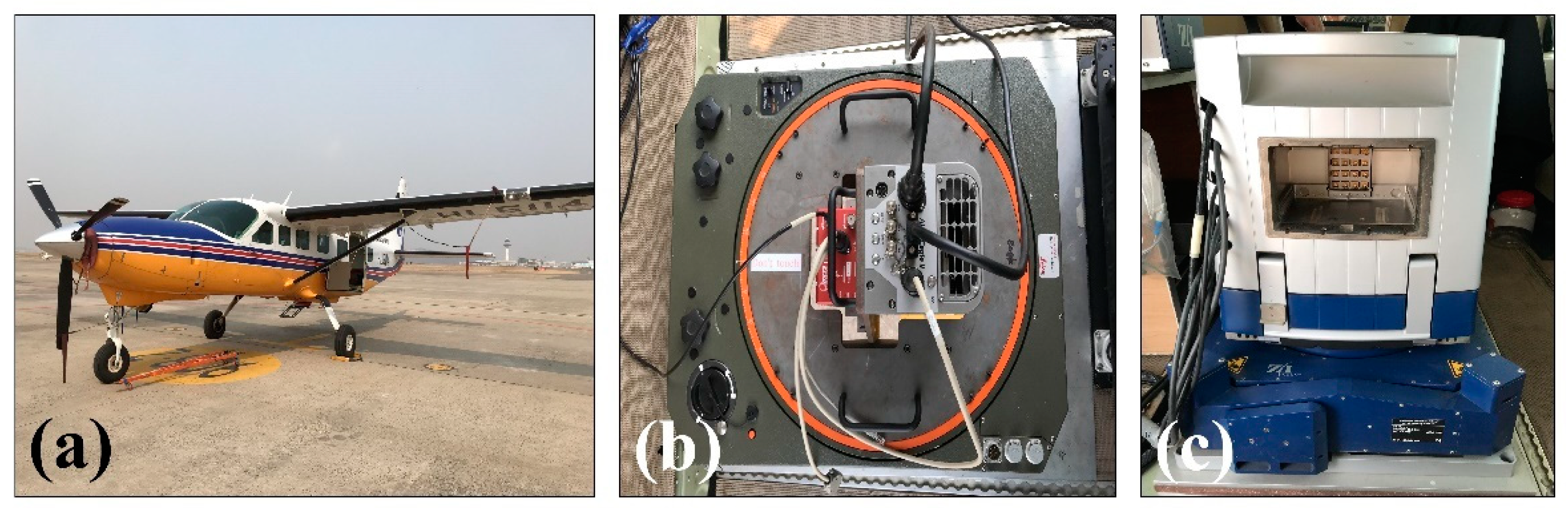
To observe high-resolution hyperspectral images, including a large number of vessels, the Jeongok Port that included a yacht club on the west coast of the Korean Peninsula was selected as the observation location for this study (Figure 1a). The observation date was May 10, 2019, and the weather conditions were clear with very few clouds and temperatures ranging from 8 °C to 27 °C. Figure 1b shows a hyperspectral RGB (red: 627.06 nm, green: 533.99 nm, blue: 488.32 nm) composite image corresponding to the red box in Figure 1a. The aircraft is a medium-sized single-engine aircraft (Cessna 208 Caravan model) which has two holes to shoot the hyperspectral sensor and the digital mapping camera (DMC) simultaneously (Figure 2). The flight speed was approximately 260 km h−1, allowing stable flight at low altitudes. The airborne observation was performed at an altitude of approximately 1 km. The hyperspectral sensor is an AisaEAGLE sensor manufactured by Specim and has a wavelength range of 400–900 nm with 127 spectral channels. The spatial resolution of the hyperspectral image at an altitude of 1 km was approximately 0.58 m and that of DMC was approximately 0.10 m. A high-resolution DMC image was used to verify the accuracy of the hyperspectral vessel detection algorithm and vessel size. Detailed specifications for the aircraft and sensors are shown in Table 1.
2.2. In-Situ Spectral Measurements
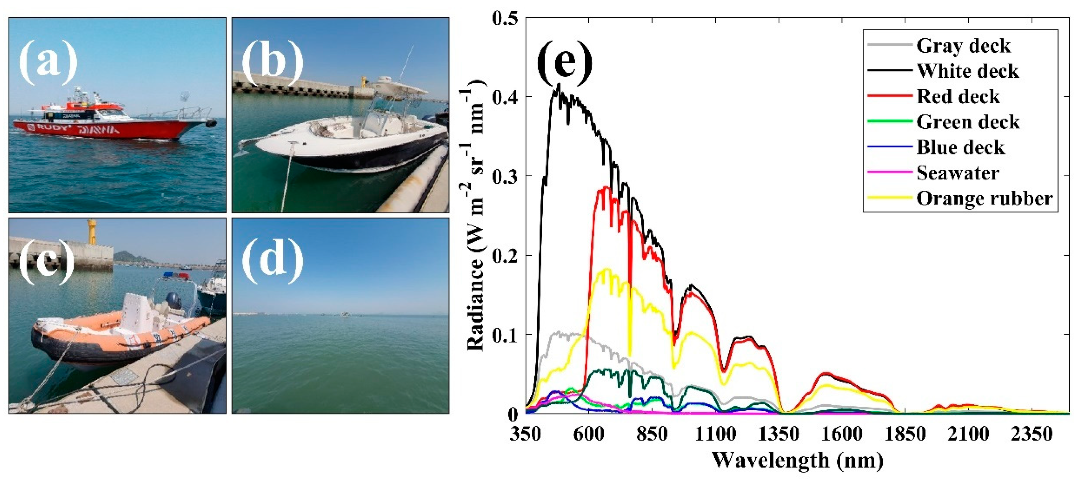
To conduct the in-situ ground experiments for obtaining hyperspectral images, we pre-positioned various vessel objects such as fishing boats, yachts, and life boats, under the path of the aircraft. Figure 3a shows a pre-deployed fishing boat for the test site, with a variety of colored deck objects in gray, white, and red. The yacht had a white deck and an orange lifeboat along the vessel boundary (Figure 3b,c). To construct the spectral library of the marine objects to be detected, the radiances of the targets were measured using a spectroradiometer. This device can measure a range of wavelengths from 300 nm to 2500 nm, with sampling intervals of 1.4 nm below 1000 nm and 1.1 nm above 1000 nm. All wavelengths were divided into 2151 channels and provided spectral information in each channel. The radiance of the white deck had a maximum value of 0.41 at approximately 480 nm, and decreased at wavelengths above 480 nm (Figure 3e). The red deck had a maximum value of 0.28 at 700 nm. The radiance increased sharply at 570 nm. Gray decks tended to decrease gradually, with their maximum radiance at 480 nm. In contrast, seawater showed a relatively small radiance of approximately 0.02 at approximately 570 nm and even lower values below 0.002 at wavelengths above 750 nm (Figure 3d,e).
2.3. Procedure for Vessel Detection Using Hyperspectral Image
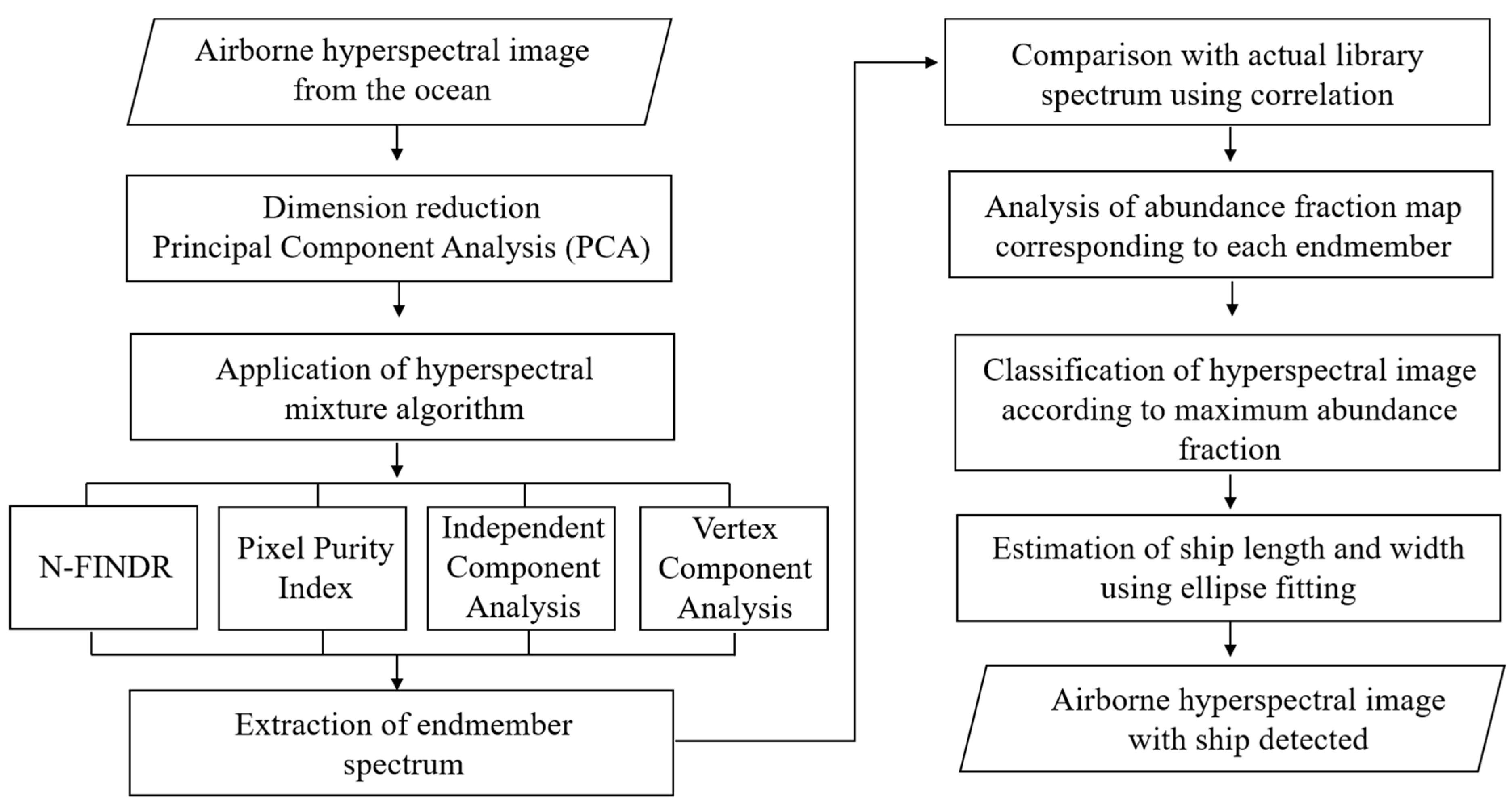
The entire procedure from hyperspectral airborne observation to the vessel detection and size estimation from an ellipse fitting method is presented in Figure 4. First, hyperspectral airborne observations surrounding the study area are performed. The principal component analysis (PCA) is applied as a pre-processing step for dimensional reduction of vessel hyperspectral images. Spectral mixture techniques including N-FINDR, pixel purity index (PPI), independent component analysis (ICA), and VCA are applied to extract the spectrum of end members of vessels and seawater for the hyperspectral images. The type of endmember can be inferred by comparing the similarity between the endmember and the marine spectrum library accumulated from in-situ measurements. Image classification based on a unit pixel can be classified through the maximum abundance fraction. Finally, the length and width of the vessels are obtained by applying ellipse fitting to the pixels classified as vessels.
2.4. Dimension Reduction Process
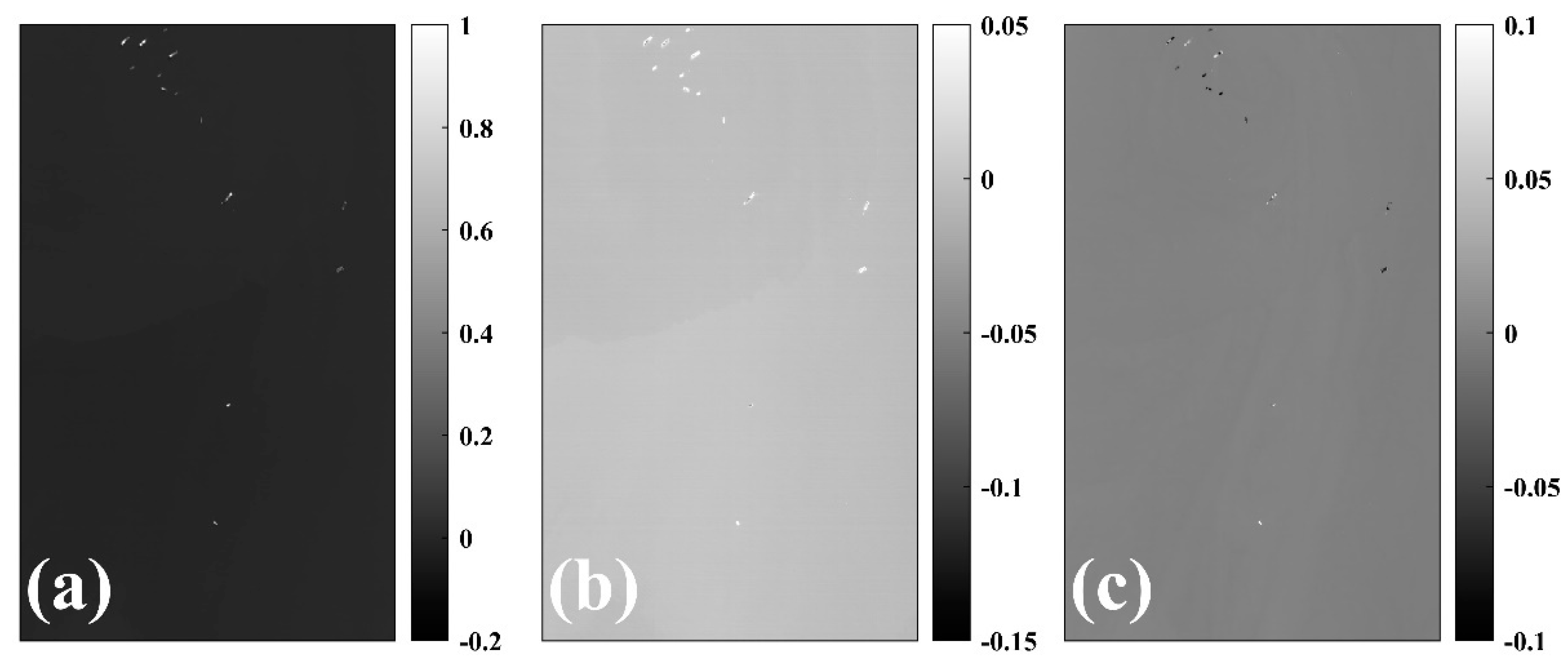
The hyperspectral image has large-capacity data containing hundreds of spectral channels, so the dimensional compression procedure should be primarily performed for efficiency of computation to extract specific information for vessel detection [39]. Typical hyperspectral compression techniques include PCA using orthogonal functions and minimum noise fraction (MNF) [40]. The PCA is a multidimensional linear transformation technique using an orthonormal basis determined by covariance, which converts high-dimensional data into low-dimensional data with no linear correlation while preserving the variance of the raw data [41]. The distance, shape, distribution, and displacement of the data are maintained when the data is orthogonally projected as a vector with a large variance. Figure 5 demonstrates the conversion of 127 bands to three representative bands by applying PCA to airborne hyperspectral images. The first mode represents 81.86% of the variance of the entire image, second mode is 4.65%, and third mode is 2.23%. The top three modes accounted for approximately 89% of the total variance.
2.5. Application of Spectral Mixture Algorithm
A unit pixel of the hyperspectral image does not contain spectral information of a single independent substance, but contains a mixture of spectral energies from one or more substances. Spectral mixture analysis is a method of classifying the mixed spectrum of different materials quantitatively in a pixel. It is hypothesized that a hyperspectral image should contain one pure substance called the endmember. Every pixel in the hyperspectral image is made up of a sum of the proportions of the endmember spectrum, and each pixel is composed of an abundance fraction of the various substances. Depending on whether the multiple endmember spectrums within a single pixel independently influence each other, they can be classified into linear and nonlinear spectral mixing. Linear spectral mixing maintains a linear relation vessel between the occupancy ratios of several endmembers in a unit pixel. Conversely, nonlinear spectral mixing is a nonlinear combination, wherein the materials of several endmembers are randomly located in a unit pixel with multiple scattering effects.
Linear spectral mixture methods include N-FINDR, PPI, ICA, and VCA. N-FINDR is one of the methods used to extract pure materials of p with the largest volume, through a random set of p pixels. Under the assumption that a simplex composed of pure material has the largest volume, p-pixel combination training was performed. This technique selects p endmembers in advance, compresses the hyperspectral image into p − 1 dimension by PCA, and constructs the pixel combinations for the compressed image. The initial p endmember set ( is used to calculate the maximum volume (V) of the endmember entities through Equation (1). Subsequently, the volume of each simplex is calculated by substituting all pixels into Equation (2) and extracting r pixels larger than the maximum volume as endmembers [42,43,44].
The advantage of this method is that it does not require any input variables other than the number of pure substances. The selection of p pure substances was determined by testing a random set of endmembers. In this study, four endmembers were selected. According to the pretests using more than five endmembers, minor parts of the endmembers overlapped and were confirmed to have similar spectra.
The PPI method repeatedly projects all pixels onto an arbitrary unit vector and then scores the pixels with extreme values [45]. The pixel with the highest score is considered an endmember, connoting that, after generating a random spectrum with the same number of bands, the spectrum distance with all pixels is calculated. Scores are assigned to the pixels with the largest and smallest values, respectively. Finally, the pixel with the highest scored is assumed to be a relatively pure material. The PPI method is not an iterative process and randomly generates k random parameters. Since this technique does not provide a criterion for selecting k parameters, the result may vary depending on the number of parameters and the number of endmembers. The endmember estimated by the PPI technique has a limitation in that it cannot represent an actual 100% hyperspectral image. It is a technique that requires a priori knowledge and experience [46].
ICA is a technique that classifies multivariate signals into subcomponents of independent signals when there is a non-Gaussian distribution of input data [47,48]. When the input signal s consisting of p is derived as a linearly mixed signal x, this technique can be expressed by Equation (3) as a process of finding p independent input signals inversely from the mixed signal. Noise ( is not distinguished from the input signal and therefore it can be omitted. The input signals are mixed matrices, and the basis vector A of the ICA method is shown in Equation (4). The ICA finds the inverse of the mixed matrix ) from the known x. The inverse mixed matrix W is required to make both the input signal and the output signal coincide (Equation (5)).
The VCA method is based on two aspects: the endmember is the vertex of the simplex and an affine transformation of a simplex is also a simplex. Similar to other algorithms, the VCA assumes the existence of a pure material in the image of which the data are projected repeatedly in the orthogonal direction in the previously determined subspace by the endmember. The signature of the new endmember matches the extremum of the projection [49,50,51].
When the endmember spectrum of the hyperspectral image is extracted through spectral mixture analysis, it is possible to analyze the abundance fraction of the endmember for each pixel. The abundance fraction should satisfy the two constraints [52]. The first constraint, abundance sum-to-one constraint, is that the sum of the abundance fractions of all pixels should be one. The second constraint, the abundance non-negative constraint, is that the abundance fraction should always have a positive value. Equation (6) is used to measure the abundance fraction of the endmember, where the pixel reconstruction error (E) should be minimized, r is the spectral signature of a pixel vector, and M is the spectral signature of the endmember. Equations (7) and (8) show least squares (LS) and fully constrained least squares (FCLS) solutions, respectively. The parameter I includes an array of p rows and one column with a component of one [44,52]. In this study, we assumed that the abundance fraction of the endmember satisfied both the fully constrained least squares conditions.
2.6. Ellipse Fitting for Vessel Size Estimation
To estimate the length and width of the vessel detected by the hyperspectral detection algorithm, we applied the ellipse fitting method [53]. This technique was designed so that the shape of the vessel boundary was most similar to an ellipse. The boundary pixels corresponding to the edge of the vessel were extracted from the magnitude of 2-D spatial gradient differences between the pixels detected by the vessel, and the surrounding background pixels of seawater. By applying the least-squared fitting of an ellipse equation to the geolocations of the boundary pixels, the characteristics of the ellipse, such as major- and minor-axis lengths, and a tilting angle, were then extracted. Here, the length and width of the vessel indicate the major- and minor axes of the ellipse.
3. Results
3.1. RGB Composite of Hyperspectral Data and DMC Image
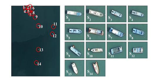
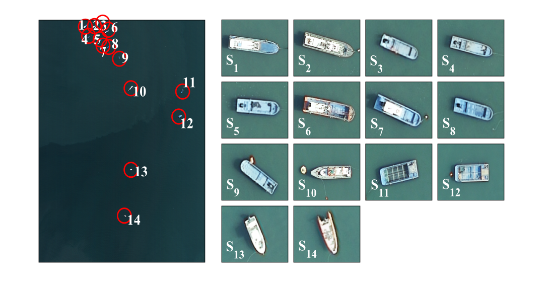
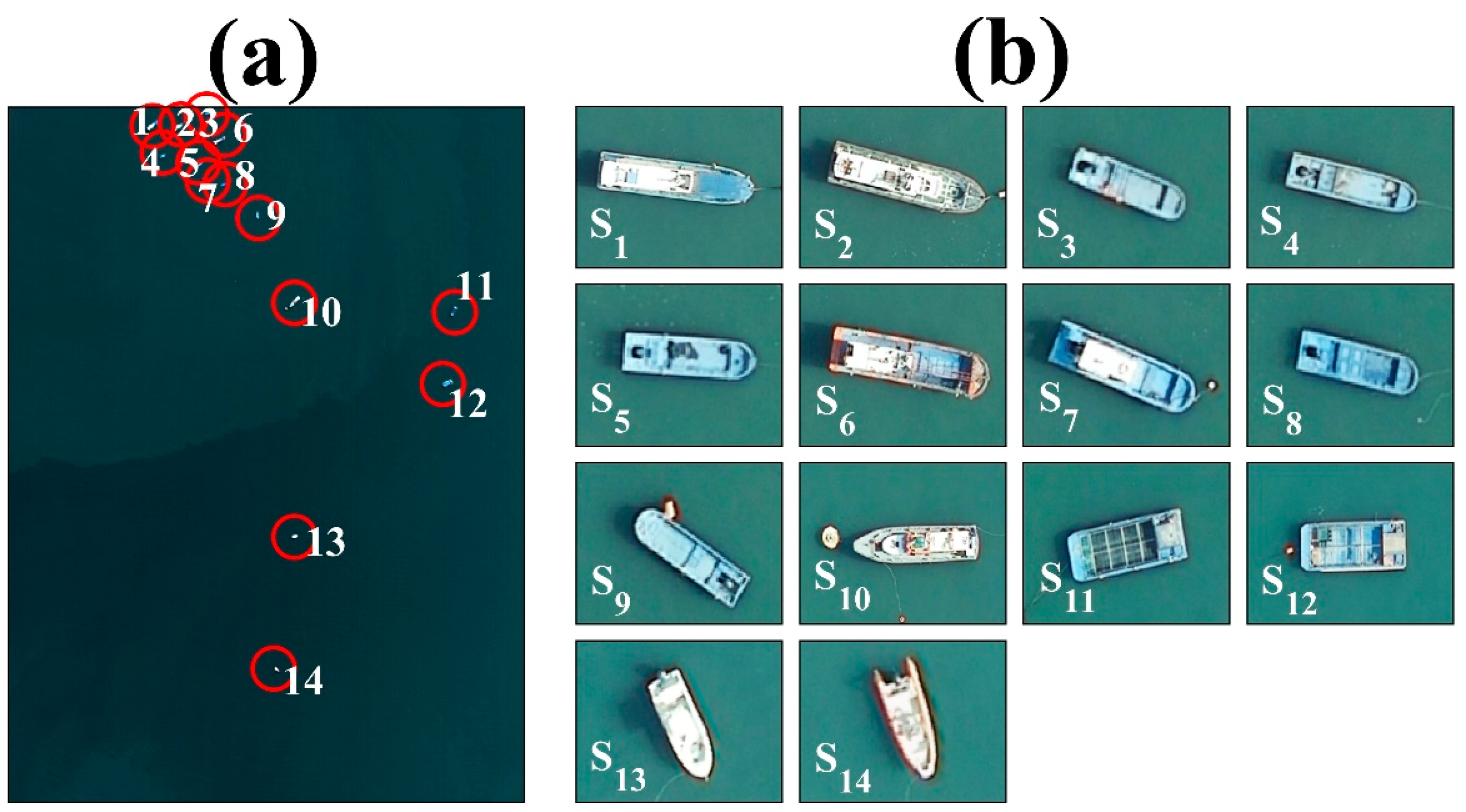
As a result of performing the composite procedure of the airborne hyperspectral data, the RGB image presents 14 vessels (Figure 6a). They are mostly concentrated in the upper portion near the port. To validate the results of the hyperspectral image analysis, a DMC image with a high resolution of 0.10 m was used. The DMC image presents the exact position of the vessels and a total of 10 fiber-reinforced plastic (FRP) vessels with blue decks (S1, S3−S9, S11, and S12) (Figure 6b). It reveals the shapes and detailed structures of every vessel. For example, the S2 vessel is a fishing boat with a white steering wheel on a gray deck. S10 is also a fishing boat with mostly gray decks and some white steering with red and green structures on the roof. S13 is a yacht with a single white deck, and S14 is a lifeboat with a white deck and an orange border. S10, S13, and S14 are pre-arranged for validation, as shown in Figure 3a–c, respectively.
3.2. Application of the Four Spectral Mixture Algorithms
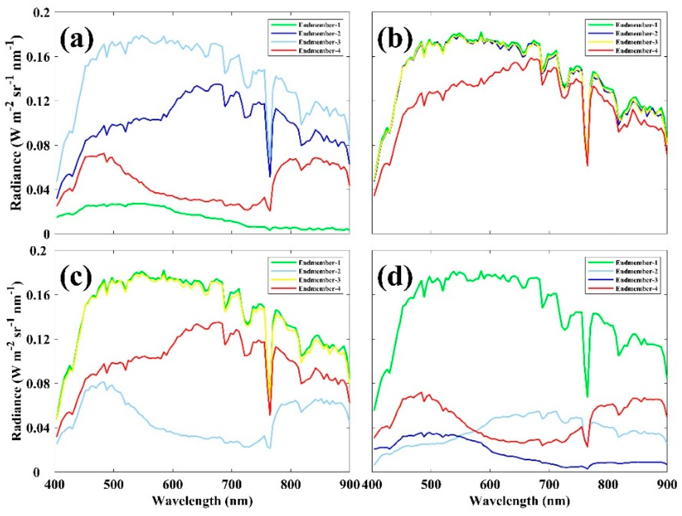
The N-FINDR, PPI, ICA, and VCA methods were applied to extract the spectra of four endmembers corresponding to single pure substances including vessels and seawater. Figure 7a shows the extracted spectra of each endmember from the hyperspectral data using the N-FINDR method. The radiance of endmember-3 showed higher values at all wavelengths than the other endmembers. The spectrum of endmember-1 (Figure 7a), showed the lowest value of 0.02 or less. Endmember-3 produced the maximum radiance at 680 nm and endmember-4 showed double peaks at 480 nm and 810 nm. These distinctive spectral distributions demonstrated the appropriate performance of the N-FINDR method.
In contrast, the spectral distributions of endmembers from the first to the third, extracted by applying the PPI technique, were similar in terms of magnitude and variation, with the exception of the fourth endmember that had a relatively lower radiance. These distributions suggest that the PPI method could not succeed in classifying the three endmembers. In addition, this method appeared to have failed to extract an endmember with a low value of 0.02 or less, corresponding to seawater, based on the results of the N-FINDR method.
The spectrum extracted through the ICA technique was subdivided into three spectra with some overlapping of the endmembers of 1 and 3 at all wavelengths (Figure 7c). Endmembers-2 and 4 show distinctive trends in spectral distribution. Similar to the PPI method, this technique also failed to extract endmembers with radiance values below 0.02, which was regarded as seawater. The VCA technique extracted four spectra with different radiance and tendency, similar to N-FINDR. The spectral distributions of endmember-1, with a maximum value of 0.18, and endmember-3, with a value less than 0.04, were extracted. Endmember-4 showed double peaks over all wavelengths. Endmember-2 showed a spectral pattern similar to that of the 2nd endmember of the N-FIDNR results. However, it showed a maximum value (~0.08) at a wavelength of approximately 700 nm Figure 7d.
3.3. Comparison of the Endmember Spectrum Using Spectral Correlation
The spectra of the four endmembers extracted from the VCA analysis in Figure 7d were compared with the spectrum library constructed through an in-situ experiment. The spectral correlation similarity (SCS) method was applied to estimate the correlation coefficients between in-situ measurements, and the endmember spectrum. The estimated correlation coefficients between the endmembers and the maritime library spectra are summarized in Table 2. Endmember-1, with a relatively large value with a maximum radiance of 0.18, had a high correlation coefficient of 0.53 with a white deck and 0.50 with a gray deck. Endmember-2 showed a tendency to increase in radiance in the section from 400 nm to 700 nm, with a decrease at high wavelengths greater than 700 nm (Figure 7d). This was correlated with the orange rubber corresponding to the lifeboat boundary, with a maximum correlation of 0.60, followed by 0.53 with the red deck. Endmember-3 showed a maximum correlation of 0.59 with seawater. Among the endmembers extracted from the sea, the spectrum with the lowest radiance was seawater. Endmember-4, which showed double peaks around 480 nm and 810 nm, had a high correlation of 0.60 with the blue deck of the FRP vessel.
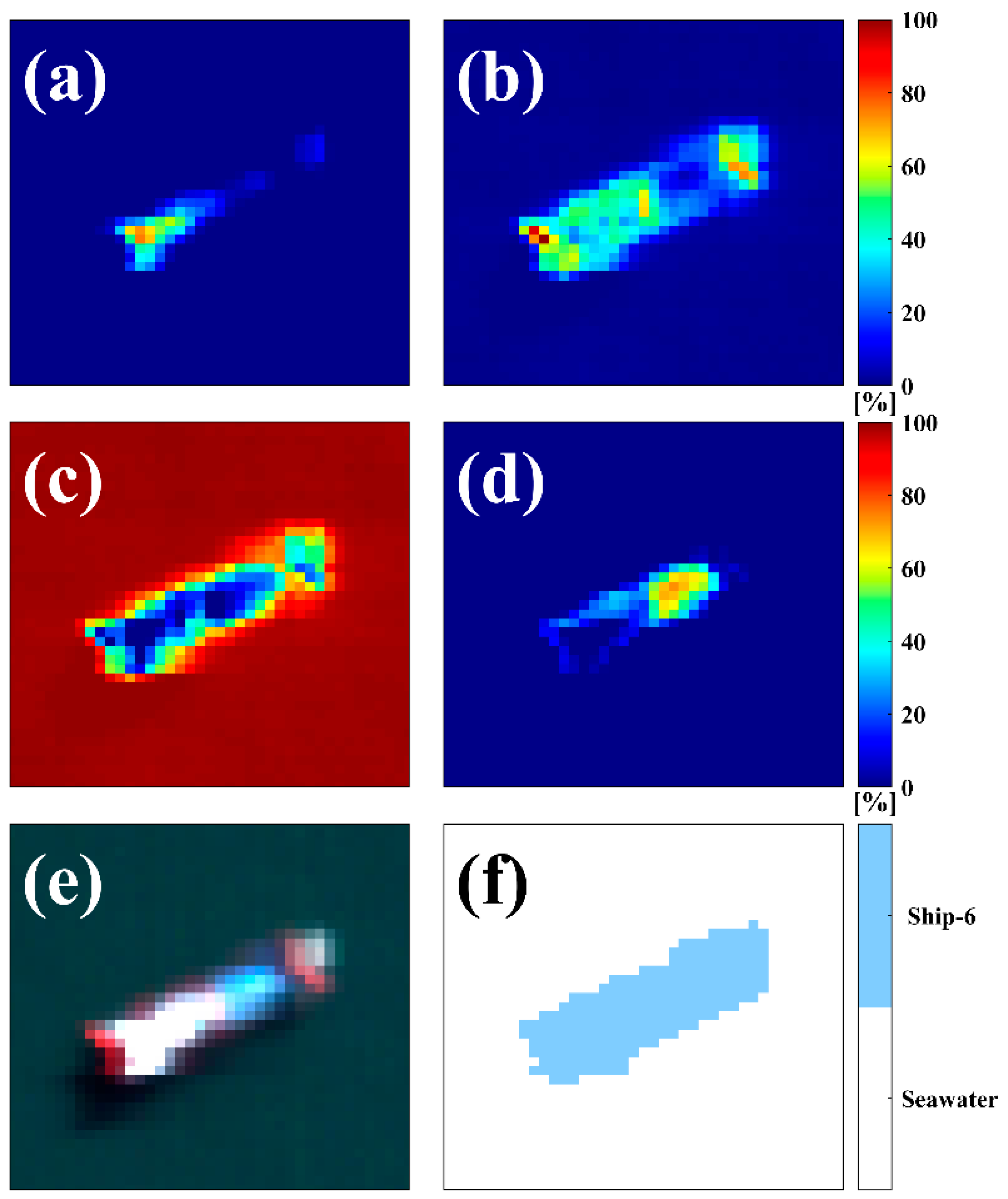
3.4. Vessel Detection Using the Abundance Fraction of Endmembers (Structure)
By comparing the abundance fractions of the four endmembers extracted by spectral mixture analysis, we analyzed the influence between the endmember spectra occupied in the unit pixel. Figure 8a–d shows the abundance fraction maps of endmember-1 to endmember-4 of the hyperspectral image including the vessel S6. Every pixel had a value between 0 and 100%. The abundance fraction of endmember-1 was greater than approximately 55% at the rear of the vessel (Figure 8a). These pixels were the positions corresponding to the vessel’s steering wheel, as marked in white in the DMC image. This is also consistent with the results of the spectral match method showing a correlation of 0.53 with the white deck. Figure 8b shows the occupancy rate of endmember-2, which accounted for more than 70% of the front and rear boundaries of the vessel. It also has percentages between 40% and 50% at the borders of both sides of the vessel. This showed a maximum correlation of 0.60 with the red objects, in comparison with the in-situ spectrum, which was similar to the positions with the same color as confirmed in the RGB composite image of Figure 8e.
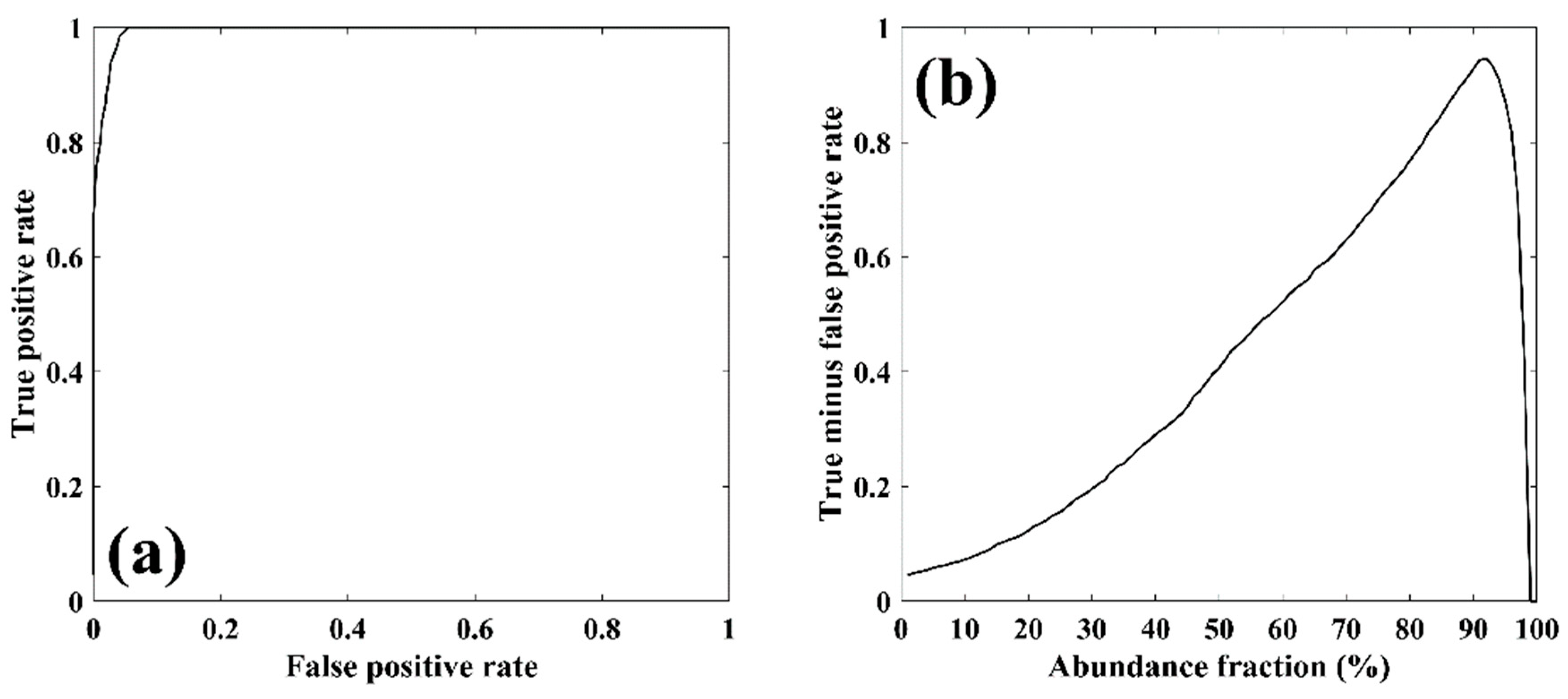
Endmember-3, with a fraction of 100% in most pixels except for the vessel in the center, corresponded to seawater (Figure 8c). This occupied more than 70% of the pixels along the vessel boundary. Pixels greater than 60% were concentrated on the front portion of the vessel, which were considered to be the pixels of the blue deck (Figure 8d). It had a high correlation of approximately 0.60 with the measured FRP blue spectrum. This result implies that the vessel and seawater can be classified based on the occupancy rate of seawater, herein endmember-3. The criterion was adopted through receiver operating characteristics (ROC) curve analysis according to the abundance fraction change, which results in a high detection probability when the true positive rate is high, and the false positive rate is low (Figure 9a) [54]. The abundance fraction that maximizes the difference between the true positive rate and the false positive rate is approximately 92% as shown in Figure 9b. The threshold was given as 90% by considering the uncertainty of the detection probability. Thus, it is concluded that the pixels occupying more than 90% of the abundance fraction of seawater were treated as seawater pixels and the rest were judged to be vessels (Figure 8f).
3.5. Accuracy Assessment of the Four Algorithms
Figure 10a demonstrates the result of detecting a vessel by the N-FINDR technique based on the endmember-1 abundance fraction corresponding to seawater. Pixels with a ratio of endmember-1 more than 90% were detected as seawater, and pixels with a lower ratio were classified as vessels.
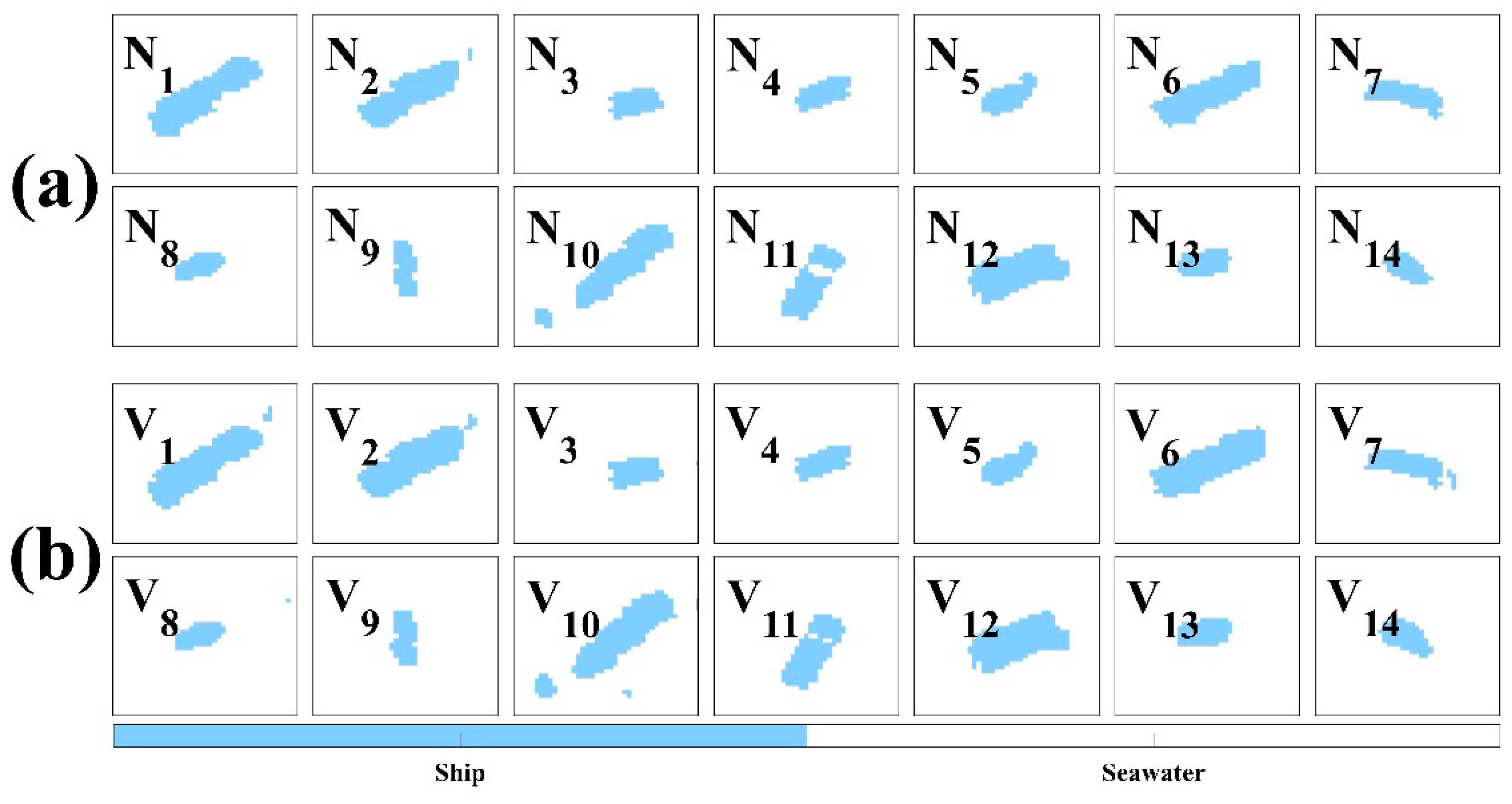
N-FINDR detected all vessels of various types and colors. This method comparatively detected the existence of vessels, however, it could not always delineate the complete shape of the vessel boundary. For example, the central portion of the N11 vessel was detected as seawater. When compared with the same vessel in the DMC image, it was inferred to be induced by the black net located at the center by being recognized as a spectrum similar to that of seawater. Therefore, it is necessary to consider that the detection accuracy depends on the structures on the surface of the vessel. In the case of the N10 vessel, some pixels of the vessel were missed at the portions of the center and the lower left. This is associated with the existence of the main rock pillar that holds the vessel. The number of pixels containing the vessel can be used to estimate the size of the vessel.
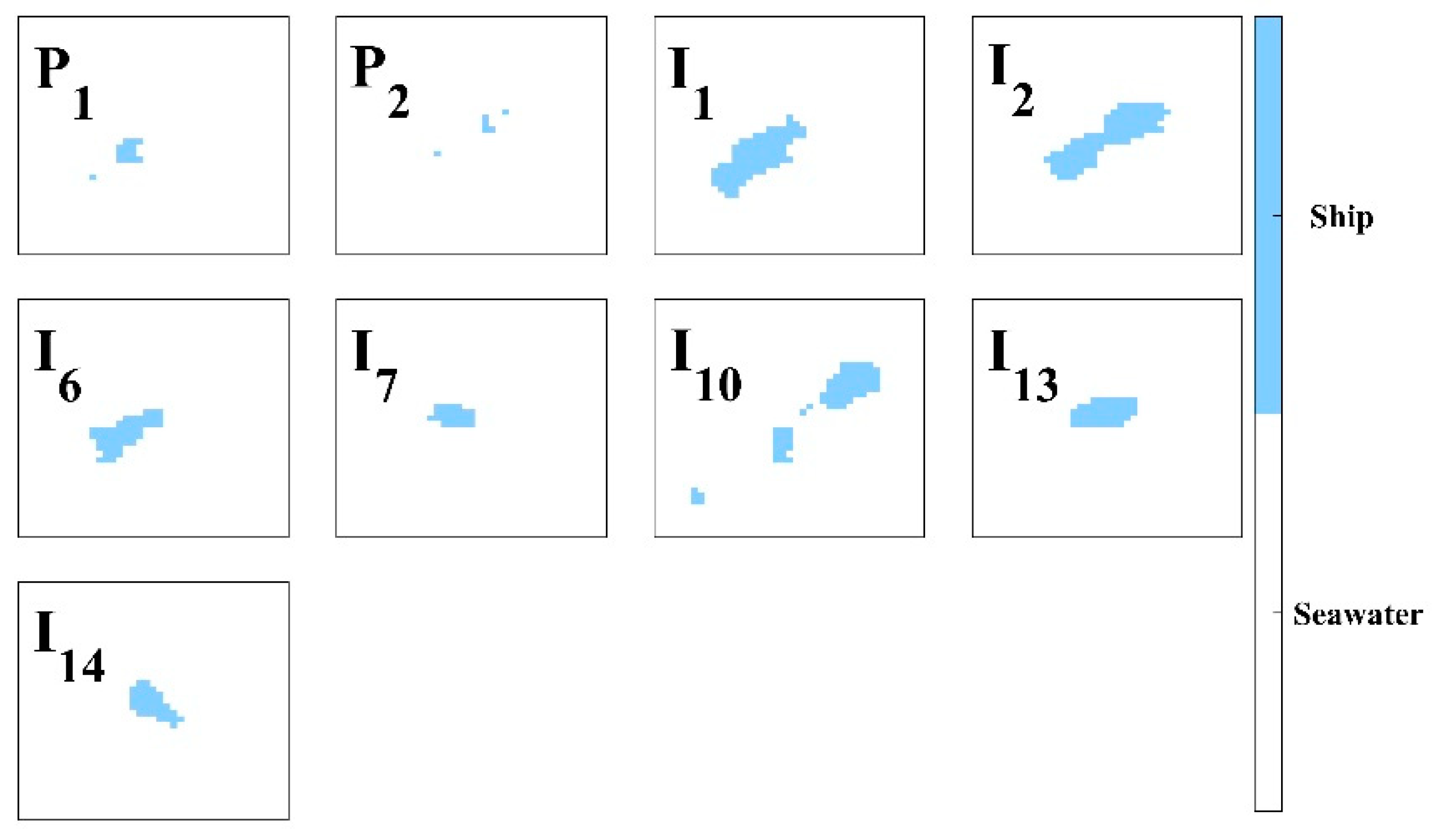
Similar to N-FINDR, the VCA technique detected 14 vessels (Figure 10b). This technique differed in radiance only in endmember-2 of the spectrum in N-FINDR, and the remainder had similar scales. As a result of classifying vessels and seawater based on 10% of the abundance fraction of endemember-3 corresponding to seawater, the pixels of the vessel boundary were detected to be more extended than those by the N-FINDR method. Similarly, some of the inside regions of the V11 vessel were classified as seawater. The results of vessel detection using the PPI and ICA techniques are presented in Figure 11. In the PPI technique, only two vessels, P1 and P2, were classified, and the number of pixels was estimated to be low, at 12 and 1, respectively. This method detected only a few parts of the vessels, which represent a low capability for vessel detection compared to other techniques. The ICA technique detected seven vessels (I1, I2, I6, I7, I10, I13, and I14) and failed to detect the other seven objects. The reason for the low accuracy of the detection by these two methods is that the four spectra extracted as endmembers were classified as not pure substances independent of each other, but impurities by both two and three endmembers.
To present the accuracy of pixel-based detection, we analyzed the histogram of the research area for the blue pixels of the RGB image to estimate the threshold value for classifying vessels and seawater. The DN values estimated to be seawater mostly ranged from 50 to 80, and the pixels estimated to be vessels clearly indicated a DN value of 255. The pixels corresponding to the boundary between the seawater and the vessel had values between 80 and 255. We assumed that pixels larger than 80 corresponded to vessels, so that a total of 1834 pixels could be found in the same vessel area. The number of vessel pixels detected by the hyperspectral mixing technique was 1768, so the probability of detection (POD) in this study was evaluated to be 96.40%, but some of the pixels tended to be overestimated compared to the actual number of vessels. Accordingly, the false alarm ratio (FAR) of the method was 4.30%. The accuracy of each vessel detection is presented in Table 3.
3.6. Estimation of Vessel Size Using the Ellipse Fitting Method
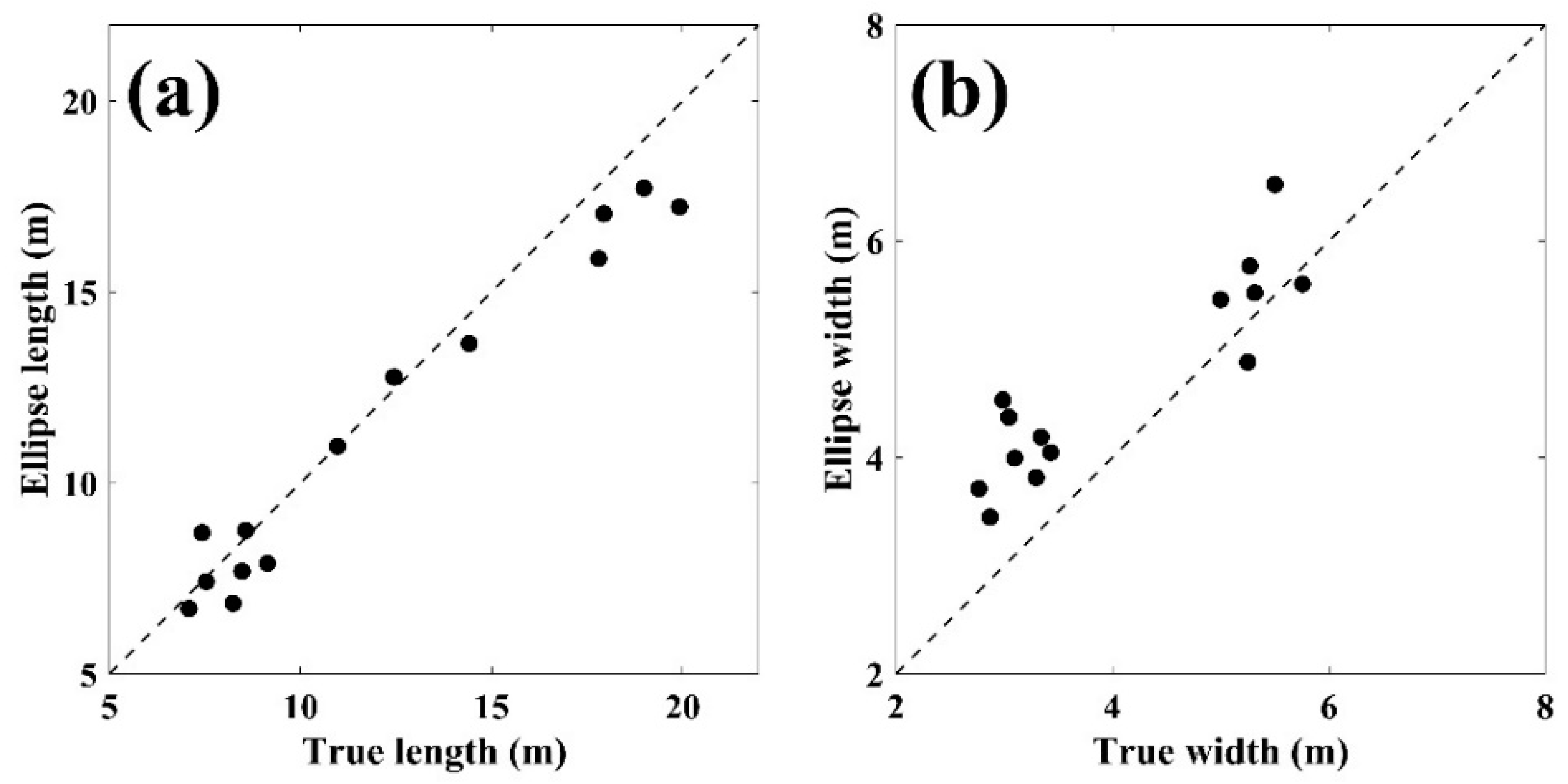
In addition to the detection of vessels using remotely sensed images, information regarding the vessel size is also a major factor in characterizing the carrying capacity of the vessel. Therefore, this study attempted to estimate vessel size by using the ellipse-fitting method. Prior to validating vessel size estimated from the ellipse method, the actual vessel size was firstly acquired for comparison using DMC images with a spatial resolution of 0.10 m. All vessels in the high-resolution image were facing in different directions, so the major axis of each vessel was rotated parallel to the horizontal direction. The difference between the maximum and minimum values of the x-axis and y-axis was regarded as the length and width of the vessel. The vessel lengths varied from 7.08 m (S14) to 19.92 m (S10), and the width of the vessels were between 2.77 m (S9) and 5.76 m (S6).
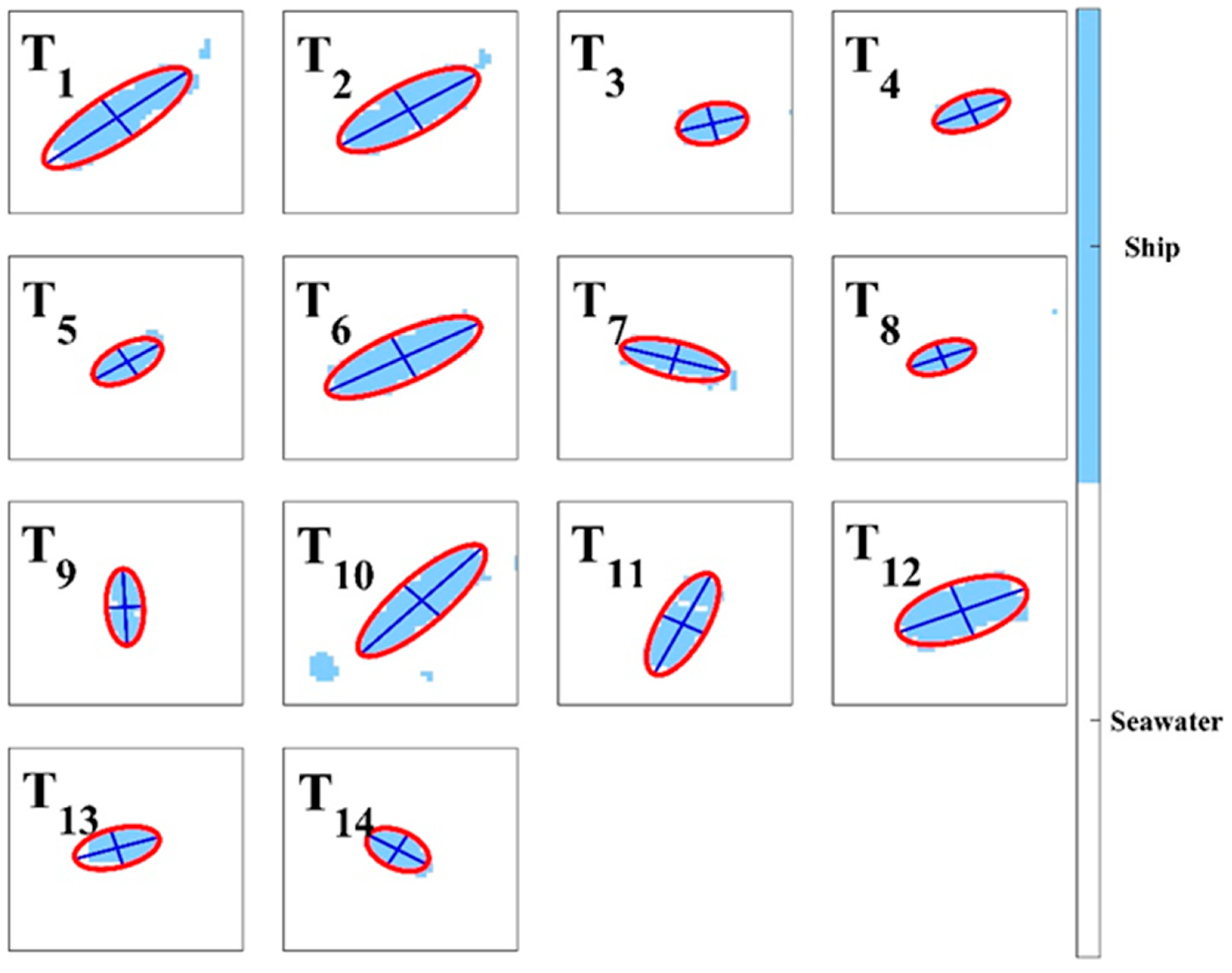
To estimate the size of the vessel pixels detected by the abundance of endmembers, pixels corresponding to the vessel boundary were selected by applying a 2-D gradient difference between the classified vessel and the seawater pixels. The red circles in Figure 12 indicate ellipses encircling the vessels, and the blue lines inside the ellipse show the lengths of the major- and minor axis of the ellipse corresponding to the vessel length and width. Figure 13 illustrates the comparison of the estimated vessel sizes from the high-resolution DMC image and ellipse fitting. The RMSE and bias of the estimated lengths were 1.19 m and 0.81 m, respectively. The estimated lengths of the vessels showed a tendency to be slightly underestimated compared with the actual length of the vessel. This tendency was found for relatively long vessels of more than 15 m. The RMSE and bias of the vessel’s width were 0.81 m and −0.63 m, respectively. The accuracy of this type of elliptic approach tends to be improved as the size of the vessel increases.
4. Discussion
This study showed a high capability of detecting the existence of vessels with high POD values, and retrieving the sizes of the vessels with comparatively good accuracy. The estimated sizes contained bias errors related to various factors and therefore, it is necessary to discuss the potential causes of the errors affecting the size estimations.
Firstly, biases can be associated with the high eccentricity of the simulated ellipse following the boundary of the vessel. A previous study has suggested that the sizes of vessels with eccentricities greater than 0.97 could likely be overestimated compared with the actual lengths [55]. Most of the eccentricity values of the vessels detected in this study were less than 0.95. Secondly, the vessels used in this study were small, being less than 20 m. The larger the vessel, the smaller the error of the calculated size. This may also be related to the size of a pixel in a remotely sensed image. In low-resolution images, small vessels are likely to contain relatively large errors as compared to large vessels. Thirdly, error can be related to the kurtosis of the vessel. In general, the front of the vessel has a sharper edge than the back position, so it offsets the overestimation when simulating an ellipse. If the front part of the vessel has a flat shape, the error will increase when simulated with an ellipse [55].
Fourthly, differences in spatial resolution between hyperspectral images and DMC images can be produced with respect to the viewing angle. The aircraft observed the sea at an altitude of approximately 1 km and an incident angle of approximately 37°. The pixel resolution decreased as the incidence angle increased from the direct point of the aircraft path to both ends of the swath. Considering the swath and angle of incidence of the aircraft, the resolution at the direct point of the aircraft was 0.58 m, whereas the resolution of the vessel pixels at both ends increased by 0.11 m. This can account for a difference of approximately 18.97% depending on the position of the vessel. Two devices with different resolutions observed the same vessel, and therefore, the vessel size contained the resolution error of each sensor itself. The size of the same vessel, observed by a hyperspectral sensor with a resolution of 0.58 m and a DMC with a resolution of 0.10 m, included respective fundamental differences in the internal resolution.
Finally, there are various types of vessels that are not suitable for ellipses. The ellipse fitting estimated the length and width of the vessel under the assumption that the boundary of the vessel was most similar to the ellipse. In the case of a closer rectangular than an ellipse, such as S12, the width of a vessel having a relatively large ratio to its length may be overestimated, particularly in terms of length. Furthermore, small vessels such as S3 have fewer pixels to be detected, so ellipse fitting is a limited in the estimation of the small size of the vessel.
5. Conclusions
In this study, airborne observations with hyperspectral sensors and DMC observations were performed to obtain hyperspectral images around the port located on the west coast of the Korean Peninsula. As a vessel detection method, spectral mixture techniques based on unit pixels such as N-FINDR, ICA, PPI, and VCA were adopted. Through this technique, four endmember spectra representing unique pixels on the images were extracted, and the correlation of each endmember was quantitatively analyzed by matching it with a maritime spectral library constructed through an in-situ experiment during the campaign. By applying the methods, the vessels were detected well, with an accuracy of approximately 96.40% for the seawater endmember pixels, and accounting for more than 90% of the abundance fraction. The spatial distribution of all endmember abundance fractions additionally suggested that the inside area of the vessel, including decks and steering wheels, could be classified with good reliability. Considering that the shape of the vessel is similar to an ellipse, the length and width of the vessels were estimated by applying elliptical fitting.
The eastern, western, and southern sides of the Korean Peninsula are surrounded by sea, thereby having a complex maritime traffic environment including various marine and port facilities, overseas trade, and high fishing intensity. Marine accidents in this region are steadily increasing over time. Considering this, it is expected that the hyperspectral remote sensing of this study will contribute to the detection of missing vessels in the event of vessel accidents as well as the management of marine vessels. This study has emphasized the importance of the high capability of hyperspectral remote sensing and airborne measurements, as well as multi-spectral remotely sensed images, in vessel monitoring and size information regarding the vessels in the coastal region. In the future, it will be necessary to analyze various spectral characteristics of ships by conducting aerial experiments using microwave SAR sensors as well as hyperspectral sensors.
Author Contributions
Conceptualization, K.-A.P.; data processing, J.-J.P.; methodology, K.-A.P., P.-Y.F., and J.-J.P.; writing—original draft preparation, J.-J.P.; writing—review and editing, K.-A.P. and J.-J.P.; discussion and funding, T.-S.K., S.O., and M.L. All authors have read and agreed to the published version of the manuscript.
Funding
This research was a part of the project titled ‘Development of Management Technology for HNS Accident’, funded by the Ministry of Oceans and Fisheries, Korea. Data processing was supported by a grant from the Endowment Project of “Development of hyperspectral image analysis technology for rapid detection and identification of marine accidents based on machine learning approaches” funded by the Korea Research Institute of Ships and Ocean engineering (PES3650).
Conflicts of Interest
The authors declare no conflict of interest.
References
- Cohen, J.E.; Small, C.; Mellinger, A.; Gallup, J.; Sachs, J. Estimates of coastal populations. Science 1997, 278, 1209–1213. [Google Scholar] [CrossRef]
- Small, C.; Nicholls, R.J. A global analysis of human settlement in coastal zones. J. Cosatal Res. 2003, 19, 584–599. [Google Scholar]
- Martínez, M.L.; Intralawan, A.; Vázquez, G.; Pérez-Maqueo, O.; Sutton, P.; Landgrave, R. The coasts of our world: Ecological, economic and social importance. Ecol. Econ. 2007, 63, 254–272. [Google Scholar] [CrossRef]
- Kanjir, U.; Greidanus, H.; Oštir, K. Vessel detection and classification from spaceborne optical images: A literature survey. Remote Sens. Environ. 2019, 207, 1–26. [Google Scholar] [CrossRef]
- McDonnell, M.J.; Lewis, A.J. Ship detection from LANDSAT imagery. Photogram Eng. Rem. Sens. 1978, 44, 291–301. [Google Scholar]
- Buck, H.; Sharghi, E.; Guilas, C.; Stastny, J.; Morgart, W.; Schalcosky, B.; Pifko, K. Enhanced ship detection from overhead imagery. In Optics and Photonics in Global Homeland Security IV; Halvorson, C.S., Lehrfeld, D., Saito, T.T., Eds.; SPIE: Washington, DC, USA, 2008. [Google Scholar] [CrossRef]
- Proia, N.; Pagé, V. Characterization of a Bayesian ship detection method in optical satellite images. IEEE Geosci. Remote Sens. 2009, 7, 226–230. [Google Scholar] [CrossRef]
- Johansson, P. Small Vessel Detection in High Quality Optical Satellite Imagery; Chalmers University of Technology: Goethenburg, Sweden, 2011. [Google Scholar]
- Vachon, P.W.; Campbell, J.W.M.; Bjerkelund, C.A.; Dobson, F.W.; Rey, M.T. Ship detection by the RADARSAT SAR: Validation of detection model predictions. Can. J. Remote Sens. 1997, 23, 48–59. [Google Scholar] [CrossRef]
- Tello, M.; Lopez-Martinez, C.; Mallorqui, J.; Bonastre, R. Automatic detection of spots and extraction of frontiers in SAR images by means of the wavelet transform: Application to ship and coastline detection. In Proceedings of the IEEE IGARSS, Denver, CO, USA, 31 July–4 August 2006. [Google Scholar] [CrossRef]
- Liu, C.; Gierull, C.H. A new application for PolSAR imagery in the field of moving target indication/ship detection. IEEE Trans. Geosci. Remote Sens. 2007, 45, 3426–3436. [Google Scholar] [CrossRef]
- Brusch, S.; Lehner, S.; Fritz, T.; Soccorsi, M.; Soloviev, A.; van Schie, B. Ship surveillance with TerraSAR-X. IEEE Trans. Geosci. Remote Sens. 2011, 49, 1092–1103. [Google Scholar] [CrossRef]
- Wang, S.; Wang, M.; Yang, S.; Jiao, L. New hierarchical saliency filtering for fast ship detection in high-resolution SAR images. IEEE Trans. Geosci. Remote Sens. 2016, 55, 351–362. [Google Scholar] [CrossRef]
- Song, S.; Xu, B.; Yang, J. Ship detection in polarimetric sar images via variational bayesian inference. IEEE J-STARS 2017, 10, 2819–2829. [Google Scholar] [CrossRef]
- Wackerman, C.C.; Friedman, K.S.; Pichel, W.G.; Clemente-Colón, P.; Li, X.A. Automatic detection of ships in RADARSAT-1 SAR imagery. Can. J. Remote Sens. 2001, 27, 568–577. [Google Scholar] [CrossRef]
- Liao, M.; Wang, C.; Wang, Y.; Jiang, L. Using SAR images to detect ships from sea clutter. IEEE Geosci. Remote Sens. 2008, 5, 194–198. [Google Scholar] [CrossRef]
- An, W.; Xie, C.; Yuan, X. An improved iterative censoring scheme for CFAR ship detection with SAR imagery. IEEE Trans. Geosci. Remote Sens. 2013, 52, 4585–4595. [Google Scholar] [CrossRef]
- Brando, V.E.; Lovell, J.L.; King, E.A.; Boadle, D.; Scott, R.; Schroeder, T. The potential of autonomous ship-borne hyperspectral radiometers for the validation of ocean color radiometry data. Remote Sens. 2016, 8, 150. [Google Scholar] [CrossRef] [Green Version]
- Rostami, M.; Kolouri, S.; Eaton, E.; Kim, K. Deep transfer learning for few-shot sar image classification. Remote Sens. 2019, 11, 1374. [Google Scholar] [CrossRef] [Green Version]
- Gao, F.; Shi, W.; Wang, J.; Yang, E.; Zhou, H. Enhanced feature extraction for ship detection from multi-resolution and multi-scene synthetic aperture radar (SAR) images. Remote Sens. 2019, 11, 2694. [Google Scholar] [CrossRef] [Green Version]
- Chen, S.; Zhang, J.; Zhan, R. R2FA-Det: Delving into high-quality rotatable boxes for ship detection in SAR images. Remote Sens. 2020, 12, 2031. [Google Scholar] [CrossRef]
- Song, J.; Kim, D.J.; Kang, K.M. automated procurement of training data for machine learning algorithm on ship detection using ais information. Remote Sens. 2020, 12, 1443. [Google Scholar] [CrossRef]
- Hirano, A.; Madden, M.; Welch, R. Hyperspectral image data for mapping wetland vegetation. Wetlands 2003, 23, 436–448. [Google Scholar] [CrossRef]
- Pengra, B.W.; Johnston, C.A.; Loveland, T.R. Mapping an invasive plant, Phragmites australis, in coastal wetlands using the EO-1 Hyperion hyperspectral sensor. Remote Sens. Environ. 2007, 108, 74–81. [Google Scholar] [CrossRef]
- Zomer, R.J.; Trabucco, A.; Ustin, S.L. Building spectral libraries for wetlands land cover classification and hyperspectral remote sensing. J. Environ. Manag. 2009, 90, 2170–2177. [Google Scholar] [CrossRef] [PubMed]
- Prospere, K.; McLaren, K.; Wilson, B. Plant species discrimination in a tropical wetland using in situ hyperspectral data. Remote Sens. 2014, 6, 8494–8523. [Google Scholar] [CrossRef] [Green Version]
- Griffin, M.K.; Burke, H.H.K. Compensation of hyperspectral data for atmospheric effects. Linc. Lab. J. 2003, 14, 29–54. [Google Scholar]
- Gao, B.C.; Montes, M.J.; Ahmad, Z.; Davis, C.O. Atmospheric correction algorithm for hyperspectral remote sensing of ocean color from space. Appl. Opt. 2000, 39, 887–896. [Google Scholar] [CrossRef] [Green Version]
- Gao, B.C.; Montes, M.J.; Davis, C.O.; Goetz, A.F. Atmospheric correction algorithms for hyperspectral remote sensing data of land and ocean. Remote Sens. Environ. 2009, 113, 17–24. [Google Scholar] [CrossRef]
- Kruse, F.A.; Boardman, J.W.; Huntington, J.F. Comparison of airborne hyperspectral data and EO-1 Hyperion for mineral mapping. IEEE Trans. Geosci. Remote Sens. 2003, 41, 1388–1400. [Google Scholar] [CrossRef] [Green Version]
- Neville, R.A.; Levesque, J.; Staenz, K.; Nadeau, C.; Hauff, P.; Borstad, G.A. Spectral unmixing of hyperspectral imagery for mineral exploration: Comparison of results from SFSI and AVIRIS. Can. J. Remote Sens. 2003, 29, 99–110. [Google Scholar] [CrossRef]
- Bishop, C.A.; Liu, J.G.; Mason, P.J. Hyperspectral remote sensing for mineral exploration in Pulang, Yunnan Province, China. Int. J. Remote Sens. 2011, 32, 2409–2426. [Google Scholar] [CrossRef]
- Lee, Z.; Carder, K.L.; Mobley, C.D.; Steward, R.G.; Patch, J.S. Hyperspectral remote sensing for shallow waters: 2. Deriving bottom depths and water properties by optimization. Appl. Opt. 1999, 38, 3831–3843. [Google Scholar] [CrossRef] [Green Version]
- Brando, V.E.; Dekker, A.G. Satellite hyperspectral remote sensing for estimating estuarine and coastal water quality. IEEE Trans. Geosci. Remote Sens. 2003, 41, 1378–1387. [Google Scholar] [CrossRef]
- Randolph, K.; Wilson, J.; Tedesco, L.; Li, L.; Pascual, D.L.; Soyeux, E. Hyperspectral remote sensing of cyanobacteria in turbid productive water using optically active pigments, chlorophyll a and phycocyanin. Remote Sens. Environ. 2008, 112, 4009–4019. [Google Scholar] [CrossRef]
- Wang, Z.; Yin, Q.; Li, H.; Hu, B. Surface ship target detection in hyperspectral images based on improved variance minimum algorithm. In Proceedings of the SPIE 10033, Eighth International Conference on Digital Image Processing (ICDIP 2016), Chengu, China, 20–22 May 2016. [Google Scholar] [CrossRef]
- Yan, L.; Noro, N.; Takara, Y.; Ando, F.; Yamaguchi, M. Using hyperspectral image enhancement method for small size object detection on the sea surface. In Proceedings of the SPIE 9643, Image and Signal Processing for Remote Sensing XXI, 96430H, Toulouse, France, 15 October 2015. [Google Scholar] [CrossRef]
- Park, J.J.; Oh, S.; Park, K.A.; Foucher, P.Y.; Jang, J.C.; Lee, M.; Kang, W.S. The Ship Detection Using Airborne and In-situ Measurements Based on Hyperspectral Remote Sensing. J. Korean Earth Sci. Soc. 2017, 38, 535–545. [Google Scholar] [CrossRef]
- Farrell, M.D.; Mersereau, R.M. On the impact of PCA dimension reduction for hyperspectral detection of difficult targets. IEEE Geosci. Remote Sens. 2005, 2, 192–195. [Google Scholar] [CrossRef]
- Luo, G.; Chen, G.; Tian, L.; Qin, K.; Qian, S.E. Minimum noise fraction versus principal component analysis as a preprocessing step for hyperspectral imagery denoising. Can. J. Remote Sens. 2016, 42, 106–116. [Google Scholar] [CrossRef]
- Koonsanit, K.; Jaruskulchai, C.; Eiumnoh, A. Band selection for dimension reduction in hyper spectral image using integrated information gain and principal components analysis technique. Int. J. Mach. Learn. Comput. 2012, 2, 248. [Google Scholar] [CrossRef]
- Winter, M.E. N-FINDR: An Algorithm for Fast Autonomous Spectral End-Member Determination in Hyperspectral Data; Descour, M.R., Shen, S.S., Eds.; Imaging Spectrometry V.: Denver, CO, USA, 1999; Volume 3753, pp. 266–275. [Google Scholar] [CrossRef]
- Xiong, W.; Chang, C.I.; Wu, C.C.; Kalpakis, L.; Chen, H.M. Fast algorithms to implement N-FINDR for hyperspectral endmember extraction. IEEE J. STARS 2011, 4, 545–564. [Google Scholar] [CrossRef]
- Park, J.J.; Oh, S.; Park, K.A.; Kim, T.S.; Lee, M. Applying hyperspectral remote sensing methods to ship detection based on airborne and ground experiments. Int. J. Remote Sens. 2020, 41, 5928–5952. [Google Scholar] [CrossRef]
- Boardman, J.W.; Kruse, F.A.; Green, R.O. Mapping Target Signatures via Partial Unmixing of AVIRIS Data. In Summaries of the Fifth JPL Airborne Earth Science Workshop; JPL Publication 95–1; NASA Jet Propulsion Laboratory: Pasadena, CA, USA, 1995. [Google Scholar]
- Chaudhry, F.; Wu, C.C.; Liu, W.; Chang, C.I.; Plaza, A. Pixel purity index-based algorithms for endmember extraction from hyperspectral imagery. In Recent Advances in Hyperspectral Signal and Image Processing; Transworld Research Network: Kerala, India, 2006; Volume 37, pp. 29–62. [Google Scholar]
- Wang, J.; Chang, C.I. Independent component analysis-based dimensionality reduction with applications in hyperspectral image analysis. IEEE Trans. Geosci. Remote Sens. 2006, 46, 1586–1600. [Google Scholar] [CrossRef]
- Nascimento, J.M.; Dias, J.M. Does independent component analysis play a role in unmixing hyperspectral data? IEEE Trans. Geosci. Remote Sens. 2005, 43, 175–187. [Google Scholar] [CrossRef]
- Bioucas-Dias, J.M.; Nascimento, J.M.P. Estimation of signal subspace on hyperspectral data. Proc. SPIE 2005, 5982, 59820L. [Google Scholar]
- Nascimento, J.M.; Dias, J.M. Vertex component analysis: A fast algorithm to unmix hyperspectral data. IEEE Trans. Geosci. Remote Sens. 2005, 43, 898–910. [Google Scholar] [CrossRef] [Green Version]
- Lopez, S.; Horstrand, P.; Callico, G.M.; Lopez, J.F.; Sarmiento, R. A low-computational-complexity algorithm for hyperspectral endmember extraction: Modified vertex component analysis. IEEE Geosci. Remote Sens. 2011, 9, 502–506. [Google Scholar] [CrossRef]
- Heinz, D.C. Fully constrained least squares linear spectral mixture analysis method for material quantification in hyperspectral imagery. IEEE Trans. Geosci. Remote Sens. 2001, 39, 529–545. [Google Scholar] [CrossRef] [Green Version]
- Park, K.A.; Woo, H.J.; Ryu, J.H. Spatial scales of mesoscale eddies from GOCI Chlorophyll-a concentration images in the East/Japan Sea. Ocean Sci. J. 2012, 47, 347–358. [Google Scholar] [CrossRef]
- Kerekes, J. Receiver operating characteristic curve confidence intervals and regions. IEEE Geosci. Remote Sens. 2008, 5, 251–255. [Google Scholar] [CrossRef] [Green Version]
- Park, J.J.; Park, K.A.; Foucher, P.Y.; Lee, M.; Oh, S. Estimation of ship size from satellite optical image using elliptic characteristics of ship periphery. Int. J. Remote Sens. 2020, 41, 5905–5927. [Google Scholar] [CrossRef]
Figure 1.
(a) Location of the Jeongok Port, (b) enlarged portion of the red box in (a), RGB hyperspectral image taken on May 10, 2019.
Figure 1.
(a) Location of the Jeongok Port, (b) enlarged portion of the red box in (a), RGB hyperspectral image taken on May 10, 2019.

Figure 2.
(a) Cessna Grand Caravan 208B, (b) AisaEAGLE hyperspectral sensor, and (c) digital mapping camera (DMC).
Figure 2.
(a) Cessna Grand Caravan 208B, (b) AisaEAGLE hyperspectral sensor, and (c) digital mapping camera (DMC).

Figure 3.
(a) Fishing boat, (b) yacht, (c) lift boat, (d) seawater, and (e) spectral radiance of the decks of vessels and seawater as a function of wavelength.
Figure 3.
(a) Fishing boat, (b) yacht, (c) lift boat, (d) seawater, and (e) spectral radiance of the decks of vessels and seawater as a function of wavelength.

Figure 4.
Flowchart of hyperspectral image data analysis for vessel detection.

Figure 5.
Spatial distributions of (a) the first mode, (b) the second mode, and (c) the third mode of the airborne hyperspectral data from principal component analysis (PCA).
Figure 5.
Spatial distributions of (a) the first mode, (b) the second mode, and (c) the third mode of the airborne hyperspectral data from principal component analysis (PCA).

Figure 6.
(a) Hyperspectral RGB composite image and (b) enlarged portion of the red circle in (a) using digital mapping camera (DMC).
Figure 6.
(a) Hyperspectral RGB composite image and (b) enlarged portion of the red circle in (a) using digital mapping camera (DMC).

Figure 7.
Comparison of endmember spectra radiance using different spectral mixture algorithms (a) N-FINDR, (b) pixel purity index (PPI), (c) independent component analysis (ICA), and (d) vertex component analysis (VCA).
Figure 7.
Comparison of endmember spectra radiance using different spectral mixture algorithms (a) N-FINDR, (b) pixel purity index (PPI), (c) independent component analysis (ICA), and (d) vertex component analysis (VCA).

Figure 8.
Abundance fraction map (a–d) corresponding to endmembers 1–4, and (e) RGB composite image. (f) Spatial distribution of the classification result for the S6 vessel based on the abundance fraction of the seawater endmember.
Figure 8.
Abundance fraction map (a–d) corresponding to endmembers 1–4, and (e) RGB composite image. (f) Spatial distribution of the classification result for the S6 vessel based on the abundance fraction of the seawater endmember.

Figure 9.
Comparison of (a) receiver operating characteristic (ROC) curve according to the abundance fractions of vessels and (b) the difference of true minus false positive rate according the abundance fraction.
Figure 9.
Comparison of (a) receiver operating characteristic (ROC) curve according to the abundance fractions of vessels and (b) the difference of true minus false positive rate according the abundance fraction.

Figure 10.
Spatial distribution of the classification result for the hyperspectral image based on the abundance fraction of the seawater endmember using (a) N-FINDR and (b) vertex component analysis (VCA) techniques.
Figure 10.
Spatial distribution of the classification result for the hyperspectral image based on the abundance fraction of the seawater endmember using (a) N-FINDR and (b) vertex component analysis (VCA) techniques.

Figure 11.
Spatial distribution of the classification result for the hyperspectral image based on the abundance fraction of the seawater endmember using pixel purity index (PPI) and independent component analysis (ICA) techniques.
Figure 11.
Spatial distribution of the classification result for the hyperspectral image based on the abundance fraction of the seawater endmember using pixel purity index (PPI) and independent component analysis (ICA) techniques.

Figure 12.
Spatial distribution of the vessels from T1 to T14, marked in blue, and least-squared fitted ellipses along the boundary of the vessels.
Figure 12.
Spatial distribution of the vessels from T1 to T14, marked in blue, and least-squared fitted ellipses along the boundary of the vessels.

Figure 13.
Comparison of (a) length and (b) width of vessels estimated by ellipse fitting.


Table 1.
Airborne and hyperspectral sensor specifications.
| Instruments | Characteristics | Specifications |
|---|---|---|
| Cessna Grand Caravan 208B | Width (m) | 15.9 |
| Length (m) | 12.7 | |
| Height (m) | 4.7 | |
| Max takeoff weight (kg) | 3969 | |
| Takeoff run (m) | 354 | |
| Landing run (m) | 227 | |
| Endurance | 5 hr 30 min | |
| AisaEAGLE Hyperspectral sensor | Spectral range (nm) | 400−900 |
| Spectral resolution (m) | Min 3.3 | |
| Spatial resolution (m) | 0.58 | |
| Spatial pixels | 1024 | |
| Spectral channel | 127 | |
| SNR | 1250:1 |
Table 2.
Correlation coefficient between endmember and marine library spectrum.
| Correlation | Endmember-1 | Endmember-2 | Endmember-3 | Endmember-4 |
|---|---|---|---|---|
| Gray deck | 0.50 | −0.02 | 0.51 | −0.06 |
| White deck | 0.53 | 0.01 | 0.49 | −0.03 |
| Red deck | 0.01 | 0.54 | −0.56 | −0.25 |
| Green deck | 0.25 | −0.19 | 0.41 | 0.28 |
| Blue deck | −0.15 | −0.43 | 0.28 | 0.60 |
| Seawater | 0.40 | −0.19 | 0.59 | −0.01 |
| Orange rubber | 0.15 | 0.60 | −0.50 | −0.30 |
Table 3.
Accuracy of vessel detection rate (%) of each ship from S1 to S14 to hyperspectral mixture analysis methods such as N-FINDR, VCA, PPI, and ICA, where ‘Total’ represents the errors for integrating all results of the four methods.
Table 3.
Accuracy of vessel detection rate (%) of each ship from S1 to S14 to hyperspectral mixture analysis methods such as N-FINDR, VCA, PPI, and ICA, where ‘Total’ represents the errors for integrating all results of the four methods.
| Method | S1 | S2 | S3 | S4 | S5 | S6 | S7 | S8 | S9 | S10 | S11 | S12 | S13 | S14 |
|---|---|---|---|---|---|---|---|---|---|---|---|---|---|---|
| N-FINDR | 85.96 | 88.23 | 72.52 | 77.27 | 82.75 | 100 | 80.56 | 75.34 | 86.76 | 82.16 | 78.71 | 89.52 | 92.96 | 100 |
| VCA | 93.61 | 100 | 78.02 | 78.40 | 85.06 | 100 | 90.74 | 75.34 | 95.59 | 100 | 90.32 | 94.29 | 100 | 100 |
| PPI | 0.06 | 47.56 | 0 | 0 | 0 | 0 | 0 | 0 | 0 | 0 | 0 | 0 | 0 | 0 |
| ICA | 35.32 | 0 | 0 | 0 | 0 | 26.82 | 20.37 | 0 | 0 | 31.92 | 0 | 0 | 60.56 | 63.46 |
| Total | 93.61 | 100 | 78.02 | 78.04 | 85.06 | 100 | 91.67 | 75.34 | 95.59 | 100 | 91.61 | 94.29 | 100 | 100 |
© 2020 by the authors. Licensee MDPI, Basel, Switzerland. This article is an open access article distributed under the terms and conditions of the Creative Commons Attribution (CC BY) license (http://creativecommons.org/licenses/by/4.0/).
Share and Cite
MDPI and ACS Style
Park, J.-J.; Kim, T.-S.; Park, K.-A.; Oh, S.; Lee, M.; Foucher, P.-Y. Application of Spectral Mixture Analysis to Vessel Monitoring Using Airborne Hyperspectral Data. Remote Sens. 2020, 12, 2968. https://doi.org/10.3390/rs12182968
AMA Style
Park J-J, Kim T-S, Park K-A, Oh S, Lee M, Foucher P-Y. Application of Spectral Mixture Analysis to Vessel Monitoring Using Airborne Hyperspectral Data. Remote Sensing. 2020; 12(18):2968. https://doi.org/10.3390/rs12182968
Chicago/Turabian StylePark, Jae-Jin, Tae-Sung Kim, Kyung-Ae Park, Sangwoo Oh, Moonjin Lee, and Pierre-Yves Foucher. 2020. "Application of Spectral Mixture Analysis to Vessel Monitoring Using Airborne Hyperspectral Data" Remote Sensing 12, no. 18: 2968. https://doi.org/10.3390/rs12182968
Note that from the first issue of 2016, this journal uses article numbers instead of page numbers. See further details here.