Semi-Automatization of Support Vector Machines to Map Lithium (Li) Bearing Pegmatites
by
 , , and
Joana Cardoso-Fernandes
1,2,* ,
,
Ana C. Teodoro
1,2 ,
,
Alexandre Lima
1,2 and
and
Encarnación Roda-Robles
3 1
Department of Geosciences, Environment and Land Planning, Faculty of Sciences, University of Porto, Rua Campo Alegre, 4169-007 Porto, Portugal
2
Institute of Earth Sciences (ICT), Pole of University of Porto, 4169-007 Porto, Portugal
3
Departamento de Mineralogía y Petrología, University of País Vasco (UPV/EHU), Barrio Sarriena, Leioa, 48940 Bilbao, Spain
*
Author to whom correspondence should be addressed.
Remote Sens. 2020, 12(14), 2319; https://doi.org/10.3390/rs12142319
Submission received: 5 June 2020
/
Revised: 8 July 2020
/
Accepted: 17 July 2020
/
Published: 19 July 2020
(This article belongs to the Section Remote Sensing in Geology, Geomorphology and Hydrology)
Abstract
:Machine learning (ML) algorithms have shown great performance in geological remote sensing applications. The study area of this work was the Fregeneda–Almendra region (Spain–Portugal) where the support vector machine (SVM) was employed. Lithium (Li)-pegmatite exploration using satellite data presents some challenges since pegmatites are, by nature, small, narrow bodies. Consequently, the following objectives were defined: (i) train several SVM’s on Sentinel-2 images with different parameters to find the optimal model; (ii) assess the impact of imbalanced data; (iii) develop a successful methodological approach to delineate target areas for Li-exploration. Parameter optimization and model evaluation was accomplished by a two-staged grid-search with cross-validation. Several new methodological advances were proposed, including a region of interest (ROI)-based splitting strategy to create the training and test subsets, a semi-automatization of the classification process, and the application of a more innovative and adequate metric score to choose the best model. The proposed methodology obtained good results, identifying known Li-pegmatite occurrences as well as other target areas for Li-exploration. Also, the results showed that the class imbalance had a negative impact on the SVM performance since known Li-pegmatite occurrences were not identified. The potentials and limitations of the methodology proposed are highlighted and its applicability to other case studies is discussed.
1. Introduction
Recently, there has been an increasing demand for lithium (Li) as a mineral commodity driven by the electric car industry, in which Li is one of the batteries’ main components. This increasing demand will result in an intensive Li exploitation soon, and untraditional Li-exploration methods that allow exploration companies to quickly delineate potentially economic areas are to meet the market expectations. With that goal in mind, some authors have attempted to identify Li-bearing pegmatites with different remote sensing data (ASTER, Landsat-5, Landsat-8, and Sentinel-2) and different image processing techniques [1,2,3,4,5,6]. Cardoso-Fernandes, et al. [7] recently reviewed the approaches and developments made to Li-exploration using remote sensing data and image processing techniques, pointing out their weaknesses and strengths.
The study area of this work is the Fregeneda–Almendra (Salamanca, Spain—Vila Nova de Foz Côa, Portugal) region, where different Li-bearing pegmatites were mapped using ASTER, Landsat-5, Landsat-8, and Sentinel-2 data, and several image processing algorithms, such as RGB combinations, band ratios, and principal component analysis (PCA) were employed [1,2]. Although these techniques allowed to vector known Li-pegmatites and other potential areas, spectral confusion with urbanized areas or agricultural fields was noticeable. Therefore, a more powerful technique capable of vectoring Li-pegmatites with more confidence is needed, to make the use of remote sensing data in Li-exploration more significant for exploration companies.
During the last decades, there has also been a growing application of machine learning (ML) in the field of geology, either in satellite-based geological mapping [8,9,10,11,12] or in mineral prospectivity mapping [13,14,15,16]. Their growing popularity is due to their ability to outperform classical classification algorithms (e.g., [8,16]). While the use of ML to map Li-pegmatites may seem promising, two main problems can be identified beforehand: (i) pegmatites are relatively small bodies and (ii) generally have low exposition. This means that in an image classification approach, Li-pegmatites correspond to a scarce class with few training samples, and some ML algorithms are sensitive to training data size and class imbalance. Furthermore, the objectives of geological exploration are different from the objectives of Land Use/Land Cover (LULC) classification. In a LULC classification problem, all classes bear the same importance and both false positives and false negatives need to be avoided. In a geological exploration, and in this case, the Li-bearing pegmatite class is the target class. Consequently, misclassifications affecting other classes are less important. Besides, false positives (i.e., over-estimating the Li-pegmatite class) may not constitute a problem while false negatives (i.e., not identifying pixels that correspond in fact to Li-pegmatites on the ground) are serious and should be avoided.
Taking this into account, the choice of correct ML algorithms is paramount to successfully map and identify Li-pegmatites. That is why in a preliminary study in the Fregeneda–Almendra region, ML algorithms like support vector machines (SVM’s) and random forest (RF) were employed to classify Sentinel-2 images [5]. According to several authors, these algorithms, when compared with classical and other ML techniques, are less sensitive to the training size [17,18] and more capable of dealing with imbalanced datasets [19]. The preliminary results obtained in this study area [5] were unsatisfactory. Both algorithms presented overfitting problems, achieving perfect to almost perfect accuracy scores at a class level, but then failing to correctly map some classes in the whole image [5]. Moreover, the discrimination between Li-pegmatites and the host-rocks was very low which ultimately resulted in a large number of Li-pegmatite false positives [5].
Moreover, algorithm parameterization is still a major difficulty in the sense that most of the time ML algorithms cannot achieve good performance without optimization [18,19]. Therefore, we believe that the previous results can be improved through better algorithm parameterization and improvement of training data. For this improved approach, SVM’s were chosen due to their challenging optimization when compared with RF. Several models were optimized and tested, including kernelized and non-kernelized SVM. The objectives of this study were then to (i) train several SVM’s on Sentinel-2 images with different parameters to find the optimal model; (ii) assess the impact of imbalanced data through the comparison of different class-balancing strategies; and (iii) improve the previously employed methodology and delineate target areas for Li-exploration. This work also aimed to answer distinct research questions, namely: (i) how to overcome the overfitting challenges; (ii) which factors most influence the SVM performance; (iii) can the SVM classification process be automatized; (iv) what are the main challenges and benefits of using SVM in Li-pegmatite mapping; and (v) can the methodology be extrapolated to other study areas. Ultimately, this research intends to fill the literature gap by contributing to the state of the art regarding the use of ML in Li-pegmatite mapping, by clarifying how SVM can be helpful in Li-pegmatite exploration.
The Fregeneda–Almendra Pegmatite Field
The Fregeneda–Almendra (FA) pegmatite field lies within the Central Iberian Zone of the Iberian Massif, spreading from Portugal (Almendra) to Spain (La Fregeneda). The border is materialized by the Águeda river, and the pegmatite field is delimitated to the north by the Douro river and to the east by the Vilariça’s fault. The study area of this work comprises most of the FA field where different types of pegmatite dykes were defined (Figure 1) taking into account their mineralogy, morphology, and internal structure [20,21,22]. These bodies intruded on the metasedimentary rocks of the Schist-Graywacke Complex (SGC) [23,24]. To the south the syn-Variscan Mêda-Penedono-Lumbrales granitic complex outcrops. Within the more evolved aplite–pegmatites, there are four dyke-types containing Li-bearing minerals: petalite-rich, spodumene-rich, lepidolite–spodumene-rich, and lepidolite-rich. All the Li-pegmatites are discordant from the host-rock main foliation and are emplaced in the same fracture set, striking from N-S to N30 °E. The petalite-rich dykes can reach a maximum thickness of 5 m to 30 m [22,25]. The spodumene-rich dykes are very similar to the petalite ones in terms of mineralogy, attitude, and dimension, with a thickness ranging from 4 m to 15 m [22,25]. Both dyke-types present no internal zonation. The lepidolite–spodumene-rich dykes present a common internal layering and thickness usually less than 15 m [22,25]. The thinner dykes are the lepidolite-rich, with a thickness lesser than 3 m and occasionally with internal banded structure (where lepidolite-rich layers alternate with albite-rich ones) [22,25].
In the FA area, there are three locations were these Li-dykes are being exploited in open-pit mines (Figure 1). This type of excavation favors the application of remote sensing data/techniques, because it increases pegmatite exposition at the surface. Moreover, each open-pit mine exploits a different pegmatite dyke-type. The Bajoca mine, located near Almendra in the Portuguese side of the field, exploits a petalite-rich dyke with up to 30 m of thickness [22]. The Alberto mine, near La Fregeneda in Spain, exploits several spodumene-rich dykes with varying thicknesses. Despite spodumene being the predominant Li-bearing phase, primary petalite can also be found in these dykes [22]. Finally, in the Feli mine, located near the Douro river on the Spanish side of the pegmatite field, a lepidolite–spodumene-rich dike is exploited.
Currently, other complementary studies are being developed in the FA area to help target Li-mineralizations. Stream sediment analysis of more than 3000 samples is being employed on the Portuguese side to identify areas with Li-potential. Spectral studies are being conducted using a laboratory spectroradiometer to build a spectral database of Li-bearing minerals. Moreover, as stated by Cardoso-Fernandes, et al. [7], the knowledge on the alteration halos associated with Li-pegmatites could favor alteration mapping techniques, thus increasing the size of the target areas and possibly allowing to vector near-surface hidden dykes. For that, more than 70 host-rocks samples are being characterized through geochemical studies. Overall, the expected results will help to improve Li-pegmatite remote mapping capabilities. The ability to recognize Li-pegmatites remotely is of great interest to the exploration/mining industry. Firstly, it would allow to decrease the time and costs of field campaigns. Secondly, the social acceptance of mineral exploration is becoming a major concern in Europe. Consequently, less intrusive exploration methods such as remote sensing are increasingly becoming an integral part of the companies’ exploration strategies.
2. Support Vector Machines (SVM’s)
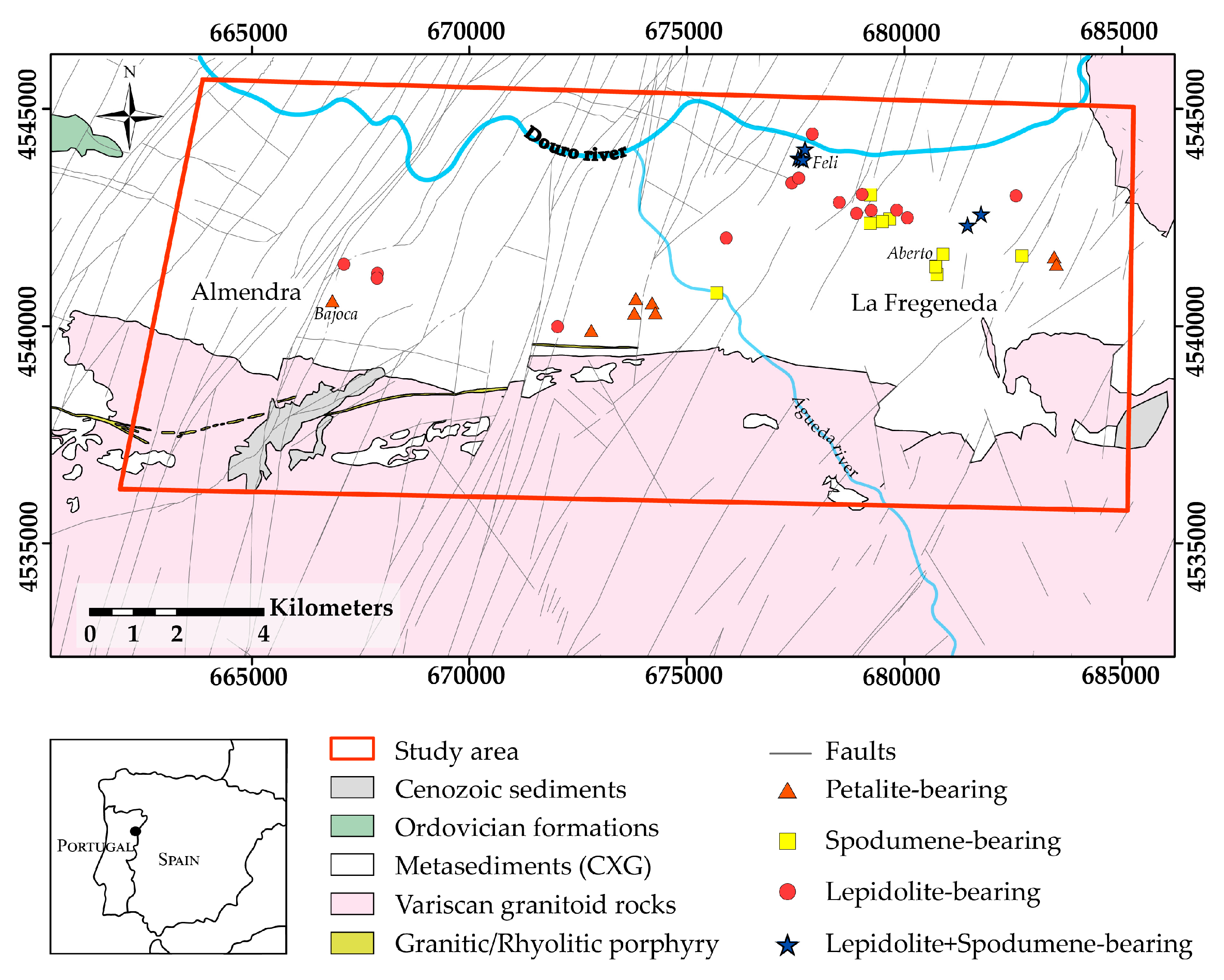
Support vector machines (SVM’s) are a non-parametric classification technique based on statistical learning theory [28], and therefore no assumption on the distribution of the data is made. The SVM technique tries to find an optimal hyperplane that separates the dataset into a defined number of classes. This optimal hyperplane is the decision boundary that maximizes the distance of the margin between the class bounding hyperplanes (also called supporting hyperplanes). The bounding hyperplanes are parallel to the optimal hyperplane and are defined by the training samples that are closest to the boundary—the support vectors (Figure 2).
SVM is by nature a binary classifier, but it can be extended for multiclass classification, using the ‘one-against-all’ or ‘one-against-one’ strategies [8,17]. In the ‘one-against-all’ strategy, k SVM models are built (where k is equal to the number of classes), each of them separating one class from the remaining. In the ‘one-against-one’ approach, k(k-1)/2 SVM classifiers are built and trained for all possible two-class combinations out of k classes [29]. In other words, a sample is classified as one of two classes for each model and the output class label is decided by the majority votes.
Since the SVM is inherently a linear classifier, it assumes that the multispectral feature data are linearly separable in the input space [17]. However, in practice, the data can be noisy and different classes may not be entirely separable due to class overlap [8,17]. This limitation can be overcome using techniques like the soft margin method [30] and the kernel trick that map the data into a higher dimension known as feature space and add additional variables called slack variables to accommodate outliers. This projection is done under the assumption that a linear boundary may exist in that higher-dimensional feature space [18]. In what concerns the soft-margin technique, the training samples are allowed to fall on the opposite side of the decision boundary (the optimal hyperplane) and the limit of the violation of the bounding hyperplanes is set by the slack variables. To each sample classified on the wrong side of the boundary, there is a penalty associated, in this case, it is the cost hyperparameter C [30]. A smaller C value will result in a larger margin that will allow for more violations, but this may lead to an inappropriate (large) number of support vectors [8,18]. Oppositely, a higher C value means a narrower margin that will limit violations. This can result in a more complex decision boundary and may cause the model to lose its generalization capability and even overfit the data [8,18]. In remote sensing, an overfitting model can explain very well the variance of the training data, while having a low capability to generalize to the whole image. Consequently, a classical sign that a model is overfitting the data is when the performance on the training set is notably better than in the testing/validation dataset [31]. In the kernel trick case, some of the more popular kernel functions(K) are, for two input vectors xi e xj:
where the γ (gamma parameter) serves as an inner product coefficient in the polynomial function (Equation (2)) and in the hyperbolic tangent function of the sigmoid kernel (Equation (4)), while controlling the kernel width in RBF (Equation (3)) [13,31]. In the specific case of the RBF kernel (Equation (3)), the γ parameter defines the range of influence of each training sample. A higher γ decreases the range of influence of sample which results in a more irregular decision boundary, while a smaller γ increases the range of influence of each sample, leading to a smoother boundary [31]. The parameter d corresponds to the degree of the polynomial function (Equation (2)). The parameter r is used for both the polynomial (Equation (2)) and sigmoid (Equation (4)) kernels, and controls in Equation (2) how much the model is influenced by high-degree polynomials versus low-degree polynomials [31].
Linear: K(xi,xj) = γxixj;
Polynomial of degree d: K(xi,xj) = (γxixj+r)d, γ > 0;
Radial basis function (RBF): K(xi,xj) = exp{– γ||xi-xj||2, γ > 0;
Sigmoid: K(xi,xj) = tanh(γxixj+r), γ > 0;
3. Data and Methodology
3.1. Dataset
As mentioned before, pegmatite exposition can be very small when compared with the spatial resolution of several free satellite products [7,32]. Despite the fact that lack of thermal band can limit the applicability of Sentinel-2 images in Li-pegmatite identification [2], its medium to high spatial resolution (10–60 m) may be crucial in a classification exercise where the target class presents the lowest exposition. Therefore, a Sentinel-2B satellite product, acquired on 07/09/2019 (tile number T29TPF), was used. The product’s processing level is 2A and its projection is Universal Transverse Mercator zone 29 N, WGS84 datum.
The Sentinel-2 mission includes a constellation of two twin satellites placed in the same sun-synchronous orbit, phased at 180° to each other: Sentinel-2A and Sentinel-2B [33]. On-board, the Multispectral Instrument (MSI) acquires information in 13 spectral bands from the visible-near infrared (VNIR) to the short-wave infrared (SWIR), but only the bands in bold in Table 1 were used in the image classification approach. These bands are the most adequate for geological purposes since minerals and rocks have important absorption features in the correspondent wavelengths. Additionally, the remaining Sentinel-2 bands have specific applications, such as detecting coastal aerosols (band 1), vegetation (bands 5, 6 and 7), water vapor (band 9), and clouds (band 10).
Since it is a Level 2A product, the bands were already provided in surface reflectance [35]. Basic pre-processing operations such as resampling all bands to a 10-m spatial resolution, as well as spectral and geographic sub-setting were performed using the Sentinel Application Platform (SNAP) software [36].
3.1.1. Sampling and Training Areas Definition
The training areas were defined based on (i) areas directly identified by visual inspection of the Sentinel-2 images, namely of a natural color composite (RGB combination 4-3-2) and the calculation of the Normalized Burn Ratio (NBR) index; (ii) extremely high-resolution images provided by Google Earth [37], Esri World Imagery [38] and by drone flights made over a known outcropping Li-pegmatite (0.025 m resolution); (iii) the Portuguese Geological Map at 1:50,000 [26,27]; and (iv) field reconnaissance.
The definition of training areas corresponded to an iterative process: for each set of training samples, class separability measurements (see Section 3.1.2) and spectral analysis were made until satisfactory results were obtained in order to select the best training areas and therefore proceed with the classification process. To improve the classification results and class separability, the number of user-defined classes was diminished when compared to previous attempts [5]. Urbanized and vegetated areas as well as the water bodies were masked out from the image, using the information provided by the Portuguese and Spanish LULC Maps (COS 2015; COS 2018; SIOSE 2014) and the Scene Classification maps provided in the Sentinel-2 Level 2A products [35]. In addition, some lithological units were deliberately left out from the classification due to small exposition (Ordovician Formations; Figure 1) or to great spatial correlation with other classes (Cenozoic sediments; Figure 1). The selected training areas contain 3053 pixels distributed by 5 classes and 33 regions of interest (ROIs) as presented in Table 2.
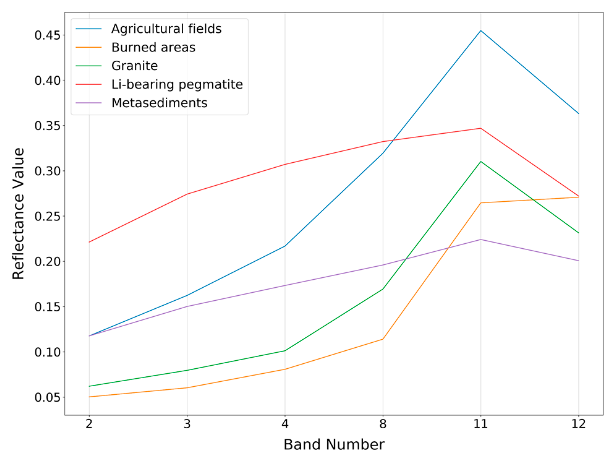
Since different classes occupy different areas on the ground, sample acquisition was not even between classes. The major problem was in the identification of samples from the Li-bearing pegmatite class because of their small exposition. Although the training areas included samples not only from the outcropping dykes, but also from ore stockpiles, the resulting dataset was still very imbalanced as can be seen in Table 2. The spectral responses of the classes for the training pixel samples were computed directly from the Sentinel-2B image—Figure 3.
3.1.2. Class Separability
As referred before, the evaluation of the spectral separability between pairs of training classes is an important step of the training areas refinement process. Therefore, a quantitative measurement of class separation was made using the Jeffries–Matusita (JM) distance and transformed divergence (TD) matrix. These spectral distances were computed using PCI’s Geomatica 2018 software [39] and the values obtained are presented in Table 3. Both distances present values between 0 and 2, where 0 means a complete overlap between the signatures of two classes, and 2 indicates a complete separation between classes [40]. In general, values higher than 1.9 indicate a very good class separability, values between 1.7 and 1.9 correspond to a good class separability, while values below 1.7 indicate that the classes are difficult to separate. These measurements can give an insight into the classification accuracy: a higher-class separability should indicate a better classification result.
Table 3 shows that all classes have a good separability, with exception of the pair Granite–Agricultural fields which is the one with minimum separability. Using the JM distance, the average separability obtained was 1.983, the minimum separability obtained was 1.865, while the maximum separability achieved was 2.000. Similarly, minimum and maximum separability obtained with the TD matrix were between 1.994 and 2.000, with an average separability of 1.999.
3.2. Parameter Tuning, Cross-Validation, and Model Evaluation
To achieve high accuracy, optimization of the parameters and kernel functions is required, because they are site-sensitive [18,19]. Parameter tuning and model evaluation was achieved using the open-source library scikit-learn [41] (version 0.20.1) for Python programming language.
Initially, all training samples were shuffled and randomly divided into training and test sets (25% for testing and 75% for training) using a stratified iterator to ensure that both sets contained samples from Li-bearing pegmatites. However, after a considerable number of trials, all the models presented the same signs of overfitting with almost perfect training scores and very high-test scores. In a classical overfitting example, the test score should be very low in comparison to the training score. However, when analyzing the results, it was possible to conclude that the training and test subsets were not independent. This means that the variance of the training and test data were very similar. Consequently, SVM not only learned very well the patterns of the training data, but also from the test subset. Only when applying the models to the whole image (i.e., when introducing new, independent data), the performance score would drop drastically as typical in overfitting models. Thus, a different strategy had to be employed to ensure that the training and testing data were independent. Considering that all samples from the same ROI would have similar spectral behavior, instead of randomly splitting the individual samples, a procedure to randomly split the ROIs into training and test subsets was adopted (Figure 4). Additional information, as well as the source code employed in this procedure, is available in Section 1 of the Supplementary Materials.
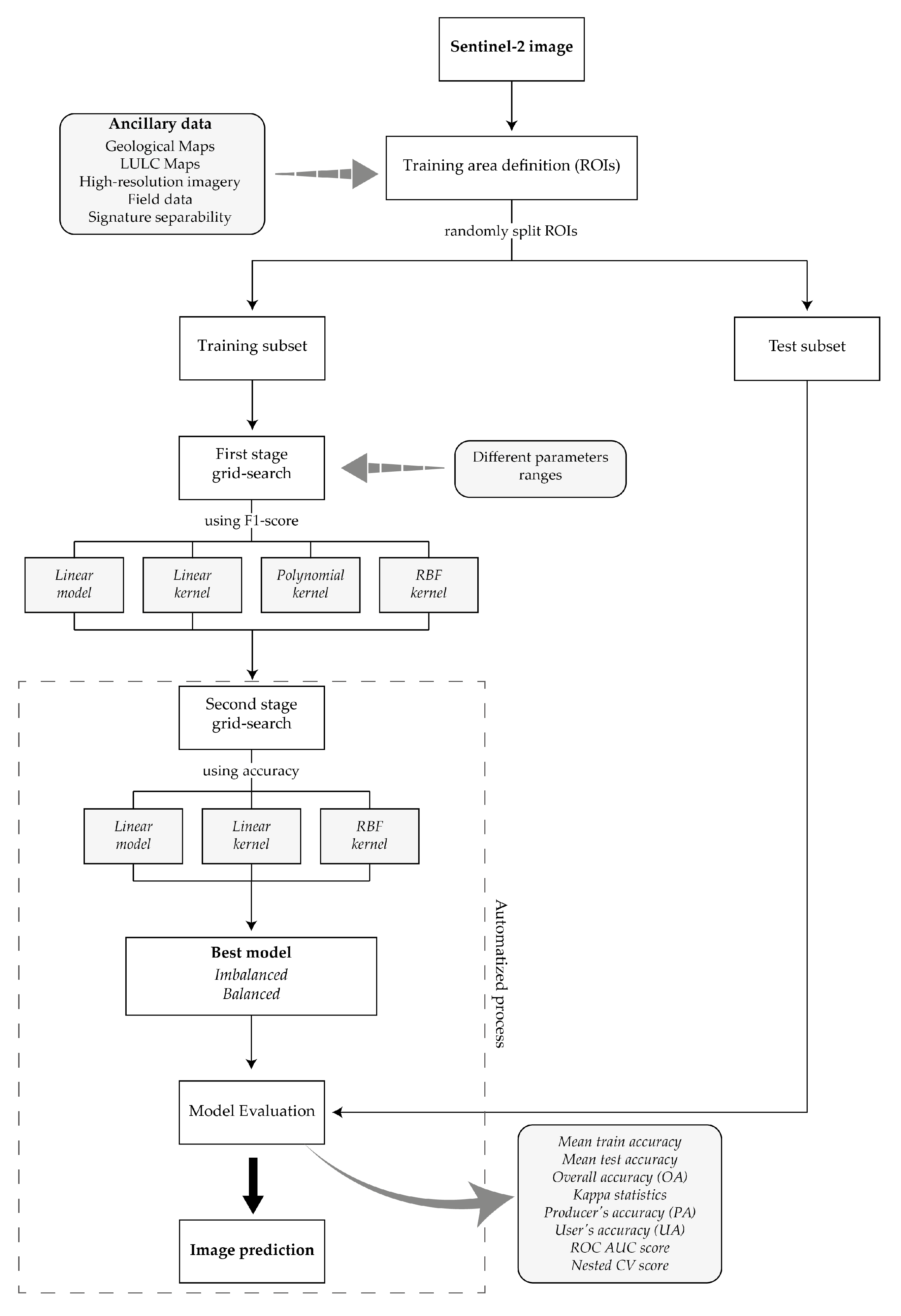
The choice of the best kernel (among linear, polynomial and RBF) and of best parameters was accomplished by a two-staged grid-search with cross-validation (CV). Besides the kernelized SVM models, the Linear model (that assumes the data is linearly separable without using any kernel function [31]) was also evaluated (Figure 4). While scikit-learn’s kernelized SVM classifier uses a ‘one-against-one’ multiclass strategy, the Linear model employs “one-vs-the-rest” [42].
The first stage grid-search represents a coarser grid-search: the Linear model (non-kernelized SVM) and all the different kernels were tested separately, using several ranges for the parameters, which either increased in a logarithmic or exponential fashion (see for example [19,43]). Each parameter range was cross-validated using a stratified 5-fold CV. This means that the original training set was split into five groups (maintaining the original proportion of samples per class), and in each fold, one group was retained in turn to use as a validation set, while the model was trained in the remaining 4/5 of the data. After the 5 folds were completed, the score obtained in each fold was averaged, obtaining the mean test score for every parameter input or combination. The best parameter(s) were the ones that obtained a higher mean CV test score. In this step, to optimize the discrimination between the target class (Li-bearing pegmatite) and the host rocks (Metasediments) the employed metric score was the F1-score of these two classes. The F1-score is the harmonic mean of precision and recall, where precision measures the accuracy of positive predictions and recall measures how many positive samples are correctly detected by the classifier [31].
The first stage grid-search is mainly based on the knowledge of the operator since different ranges will return very distinct optimal parameter(s). The sensitivity of SVM to the setting of the parameter range was already described by other authors [44]. Therefore, the results of each range should be interpreted carefully and an increase or decrease of the search space may be necessary to improve the grid-search outputs. When choosing the best range, several criteria must be considered besides the CV test score, namely the values of the returned parameter(s). This means that when the obtained scores are similar, the operator should opt for the one with a smaller C and/or gamma, for example, to avoid choosing a rigid model that may overfit the data [31].
To try to balance the dataset, three different approaches were applied: (i) use a built-in class-weight parameter; (ii) downsampling; and (iii) upsampling. In the first case, a weight is attributed to each class during the training phase to account for class imbalance: this weight can be user-defined, or it can be set automatically to the inversely proportional to class frequency (the so-called “balanced” mode). In this work, we decided to use the “balanced” option. In what concerns the downsampling process, the classes with more observations are randomly sampled without replacement, to obtain several samples equal to the size of the smallest class. On the other hand, upsampling is the process that for each observation of the largest class, randomly selects from the other classes with replacement. For more information on the first stage grid-search, see Section 2 of the Supplementary Materials.
In the second stage grid-search, a stratified 5-fold CV was again implemented, but this time with linear increments around the best parameter values returned in the first step. Whenever possible, the incremental steps employed were the same used by Oommen, et al. [43]. In this second stage, the polynomial kernel was not included, since the best degree obtained in the first stage was always equal to one, and the first-degree polynomial corresponds to the linear kernel when the parameter r equals to zero (Equations (1) and (2)). The downsampling and upsampling strategies were also excluded from the second stage, because the introduction of a random sampling process (that did not consider the ROIs) leads to overtraining problems. Consequently, in the second stage grid-search, only three models were trained for both the imbalanced and balanced data using the class-weight parameter. The choice of the best model was automatized (see Section 3 of the Supplementary Materials) and in the end, two models, one built on the imbalanced data and one using the class-weight option, were applied to the whole image (Figure 4). This means that on the contrary of what happened in the first stage (where each model was trained separately), in the second stage the three models were confronted in the same grid-search and the best model was automatically return. Only the best model returned were subjected to the “Model evaluation” step of Figure 4.
In what concerns the model evaluation, the metric score employed to choose the best model in the second stage was the accuracy. Besides the mean train accuracy and mean test accuracy obtained in the CV, the overall accuracy and the Kappa statistics were also computed. To evaluate the classification at the class level, the producer’s and user’s accuracy were calculated. Knowing the true and predicted classes of the test data, the confusion matrix gives insight for each class on how many samples were correctly classified, how many were misclassified, and on which class the samples were incorrectly classified. The matrix diagonal represents the samples that were correctly classified in the respective class and the OA is calculated by dividing the sum of the correctly classified instances by the total number of pixels [45]. The producer’s accuracy (PA) is obtained by dividing the number of correct pixels in a given class by the total number of pixels of that class in the test set, and indicates the probability of a training sample being correctly classified [46]. On the other hand, the user’s accuracy (UA) can be computed by dividing the number of correct pixels in a determined class by the total number of pixels that were classified in that class. It indicates the reliability of the map and gives the probability that a pixel classified as of belonging to a certain class actually belongs to that class on the ground [45,46]. The Kappa statistic corresponds to a measure of agreement between the classifier output and reference data [47]. To access the influence of the correct choice of model in the Li-pegmatite class, receiver operating characteristic (ROC) curves were computed for all the models tested during the second stage grid-search. The ROC curve plots the true positive rate (or for recall) against the false positive rate (fraction of negative samples misclassified as positive) [31]. The area under the curve (AUC) score was calculated to compare the different classifiers.
The ability of each model to generalize to unknown data was evaluated by applying a nested CV. This procedure allows multiple splits of CV instead of just one (the training-validation split), thus reducing the risk of biasing model evaluations by using different portions of the data for parameter selection and model evaluation. In practice, the procedure corresponds to a CV of the first CV: the inner loop is for parameter tuning and model selection, the outer loop is dedicated to evaluating the model’s performance. In this work, the outer loop consisted of a 3-fold CV. The source code employed in this procedure is available in Section 3 of the Supplementary Materials.
4. Results
The automatized process allowed to choose the best model for both the imbalanced and balanced datasets. Data balancing had an impact on SVM performance since the best model found was the Linear model (non-kernelized SVM) for the imbalanced data and the RBF kernel for the dataset balanced using the class weight option.
The results from the second stage grid-search with CV and from the model evaluation step are presented in Table 4. In general, both models reached a similar performance, although the Linear-SVM obtained a higher train score. The RBF-SVM was the model that achieved a higher test score during the CV process, but the Linear-SVM attained a better OA and Kappa hat statistics. The models’ generalization capability (nested CV score) was also very similar.
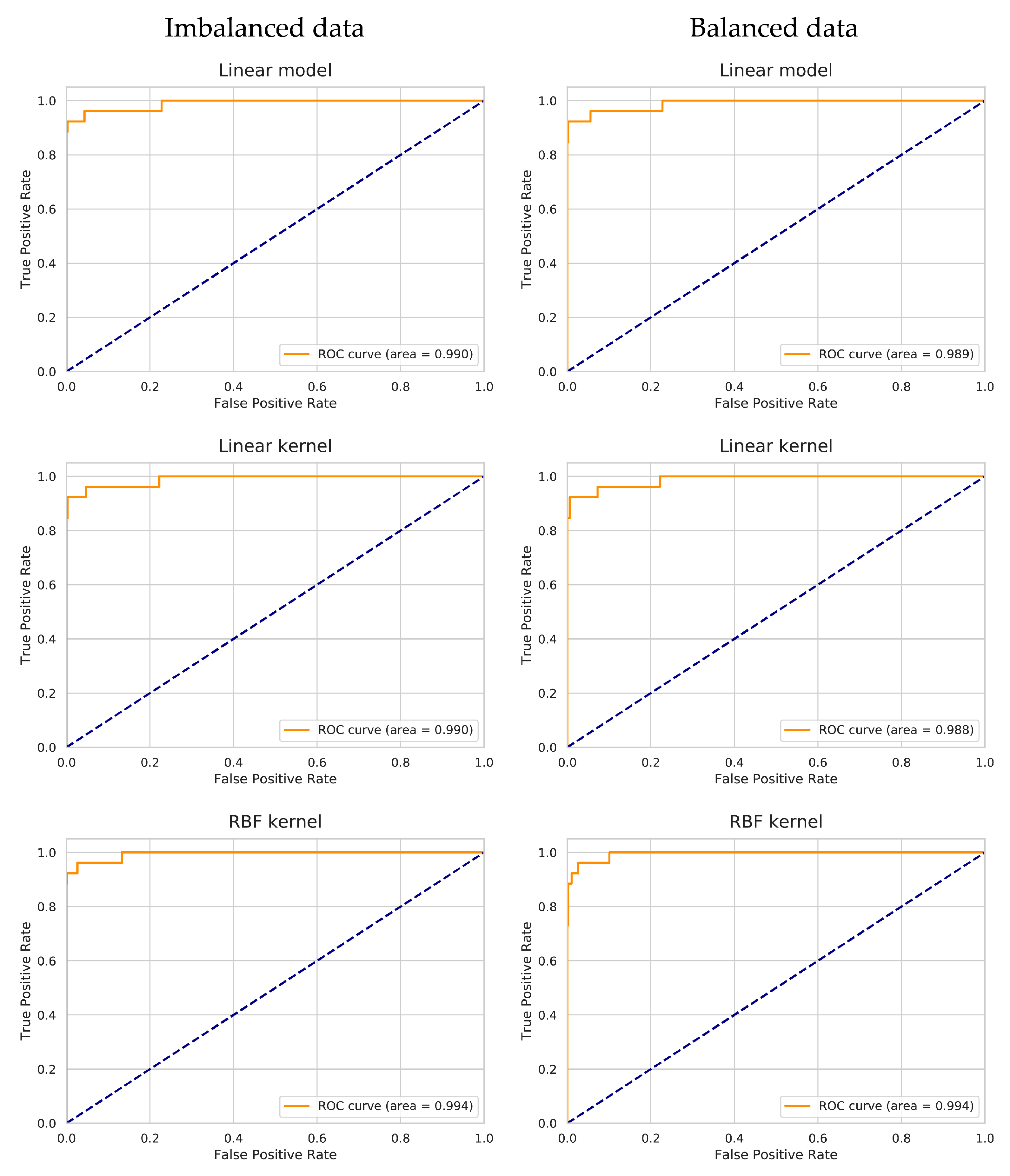
Based on the metrics, especially on the attained OA and Kappa hat, the Linear-SVM appears to be the best model. Plotting the ROC curves for each model tested in the second stage grid-search and computing the respective AUC score allowed to assess the models’ performance exclusively on the Li-pegmatite class (Figure 5). The results show that the use of class balancing strategies improved the performance on the Li-pegmatite class for the Linear model and for the Linear kernel. In the balanced dataset, the best model found through the automatized process, the RBF kernel, was the one that achieved a higher AUC. However, in the case of imbalanced data, the RBF kernel was still the one with the highest AUC, despite the Linear model being chosen as the best model with the automatized process. This happened because the automatized process selects the best model based on the performance in all classes while the AUC score only accounts for the Li-pegmatite class.
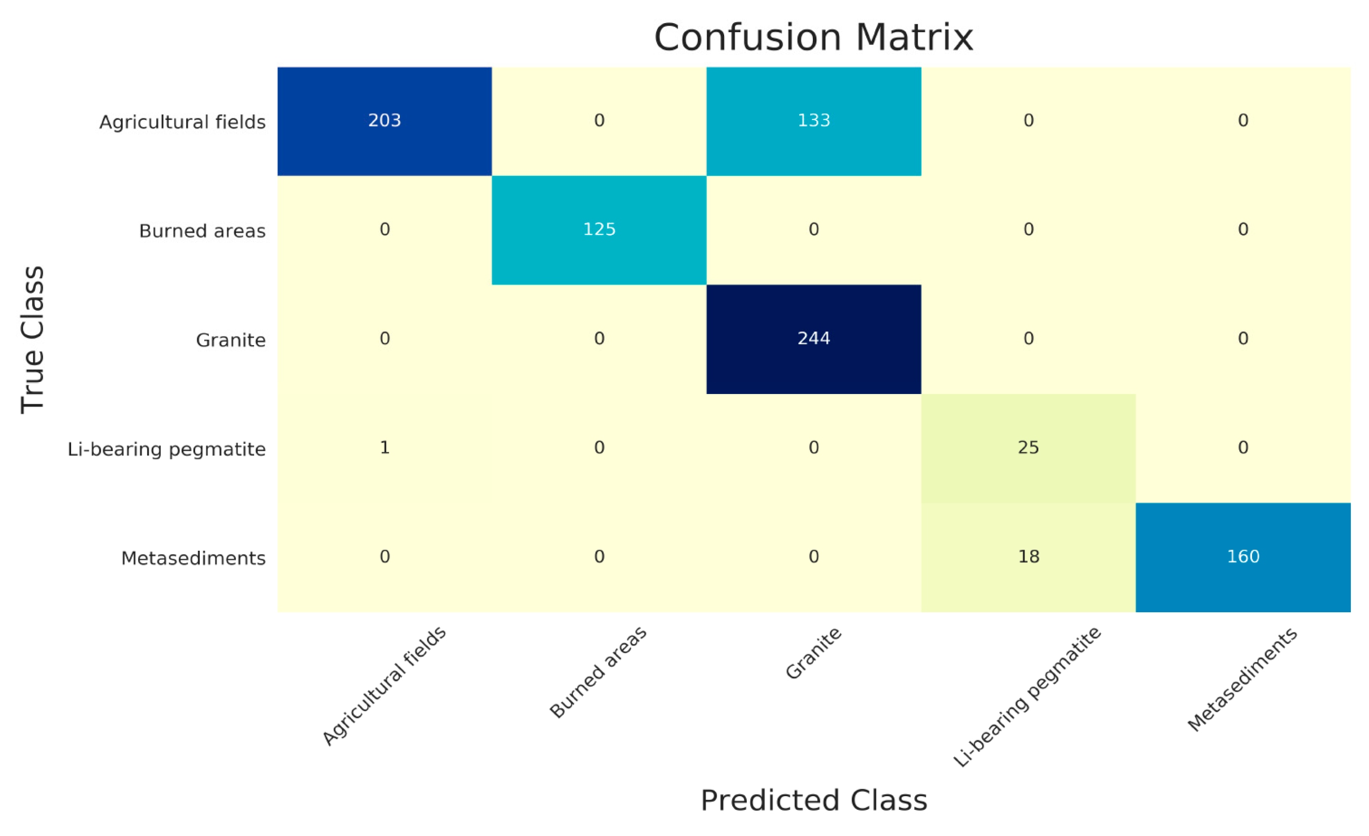
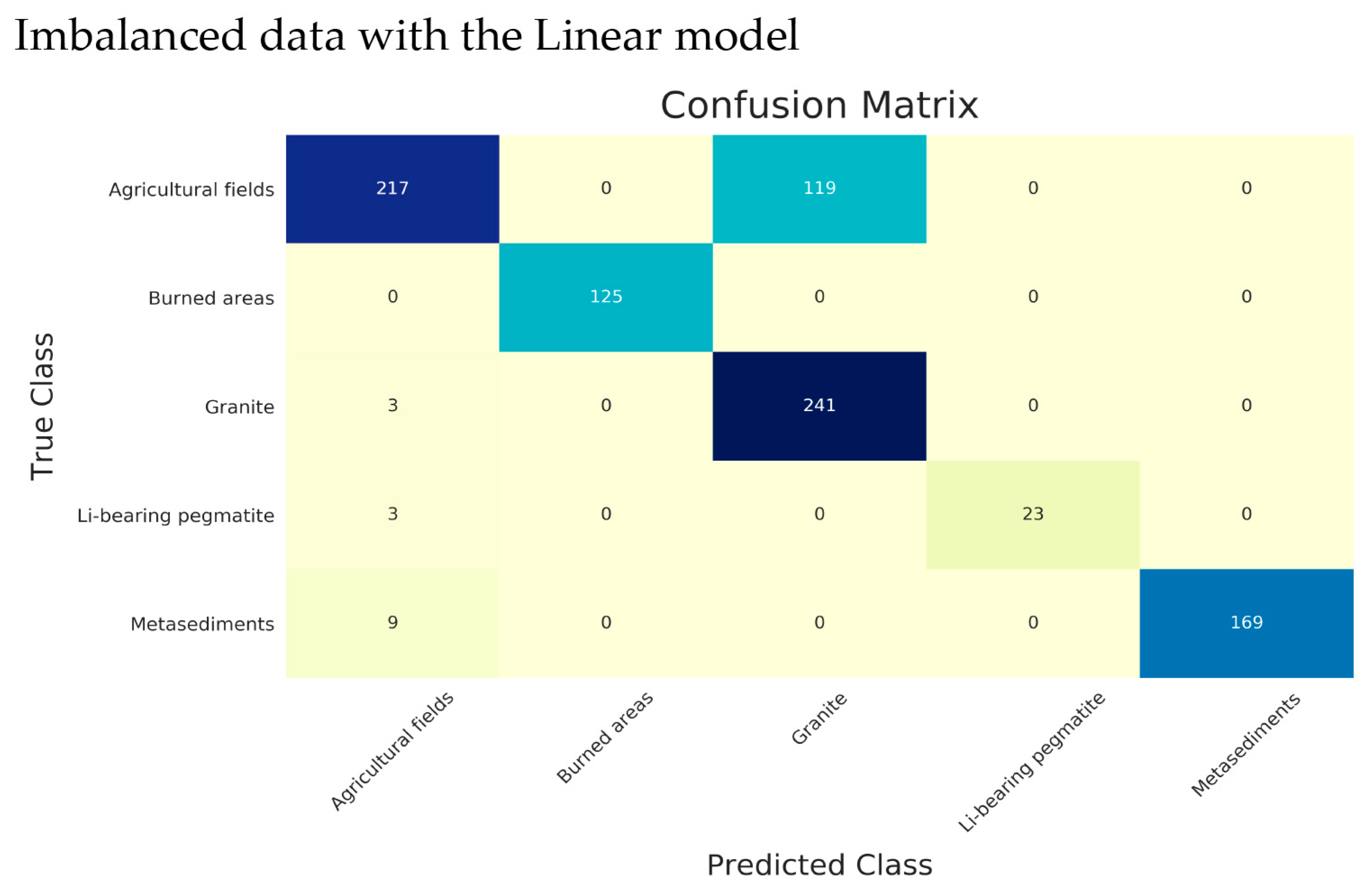
To analyze and compare in detail the accuracy performance on each class the confusion matrices were computed for the Linear-SVM (Figure A1) and the RBF-SVM (Figure 6). The UA and PA were computed considering the respective confusion matrix and are presented in Table 5.
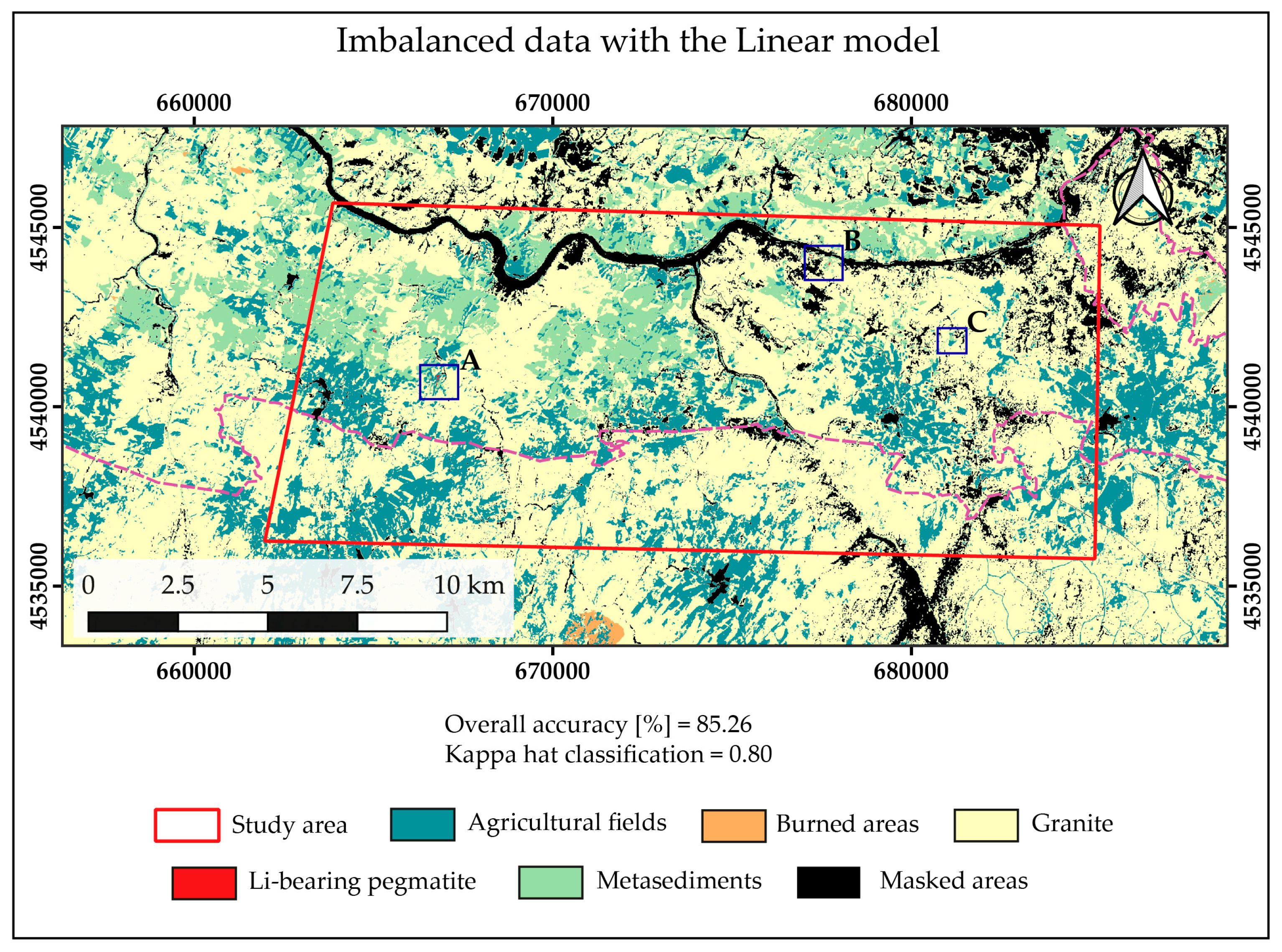
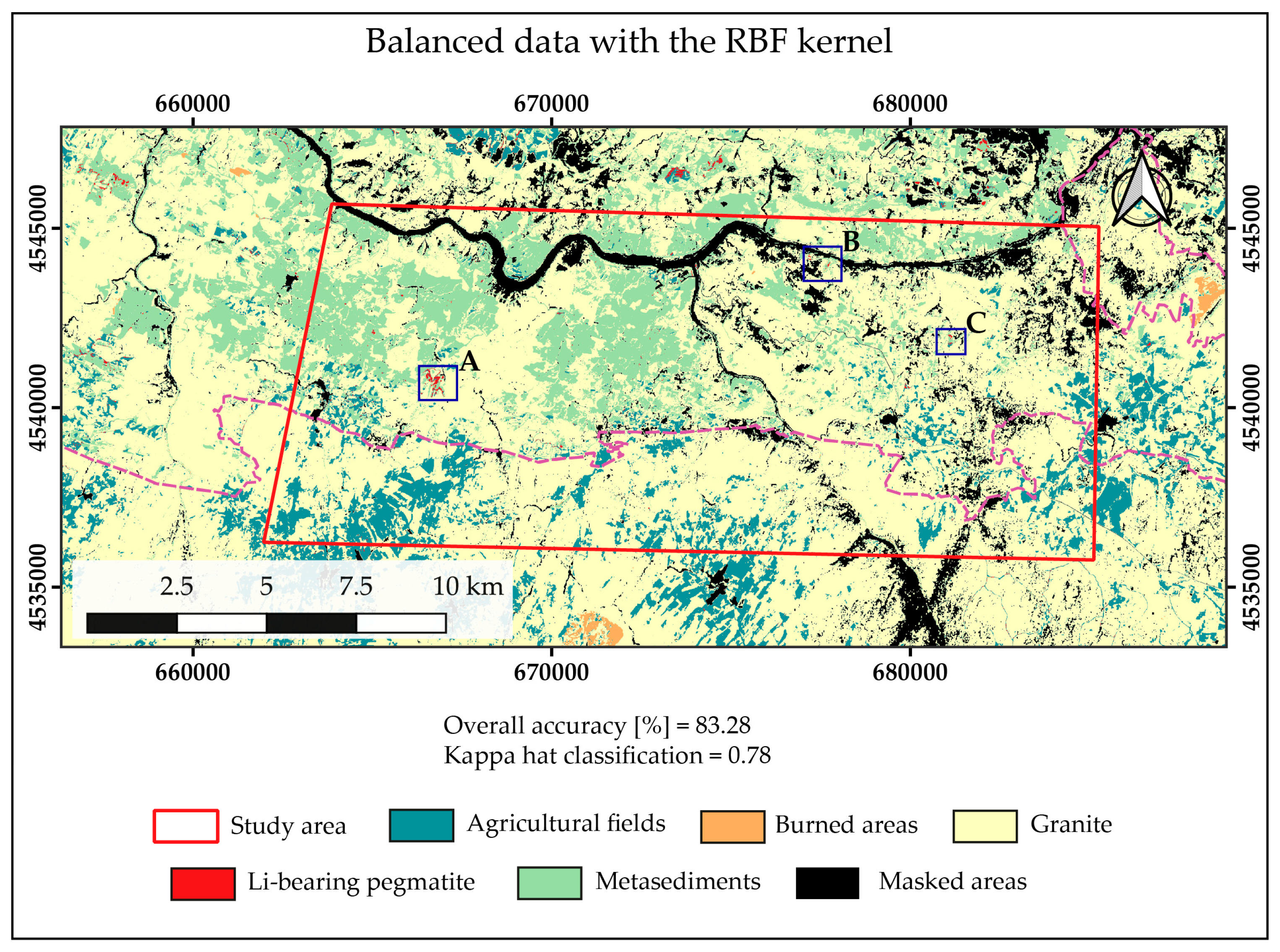
As can be observed, in both models, the greater misclassification errors happened between the Agricultural fields and Granite classes. Regarding the Li-bearing pegmatite class, the Linear-SVM model was the one that maximized the discrimination between the mineralized dykes and the host rocks, but this was done at a cost—a higher number of false negatives. Conversely, the RBF-SVM model minimized the misclassification of true samples from the Li-bearing pegmatite class at the cost of a higher confusion with the metasedimentary host-rocks. These results are in line with the interpretations with the final classification maps obtained for Linear-SVM (Figure 7) and for RBF-SVM (Figure 8).
The comparison between the two classification maps indicated that the overall performance of each class changed from one model to the other. For example, the RBF-SVM model was able to correctly classify all the areas affected by wildfires while the Linear-SVM model misclassified some of these areas as Metasediments. On the other hand, the Linear-SVM model was the one that better identified the Agricultural Fields, whereas the RBF-model only showed good performance in the classification of the Agricultural Fields located over a granitic basement. Both models showed problems in the classification of the Metasediments that were often classified as Granites.
In what concerns the target class, Li-bearing pegmatite, the Linear-SVM was able to minimize the occurrence of false positives. Therefore, the pixels classified as belonging to the Li-class were limited, almost exclusively, to small areas inside the known open-pit mines. On the other hand, the RBF-SVM was able to identify other possible target areas beyond the known occurrences. As this is the final goal of mineral exploration, the results obtained with RBF-SVM are preferred even though some areas where Metasediments outcrop were classified as Li-bearing pegmatite (top left corner and top center of the classified image—Figure 8). These results are contradictory to the quantitative model analysis achieved with the OA and Kappa statistics. That is why it is fundamental to evaluate the models using distinct statistical methods. Moreover, the results obtained with each model were qualitatively analyzed and evaluated.
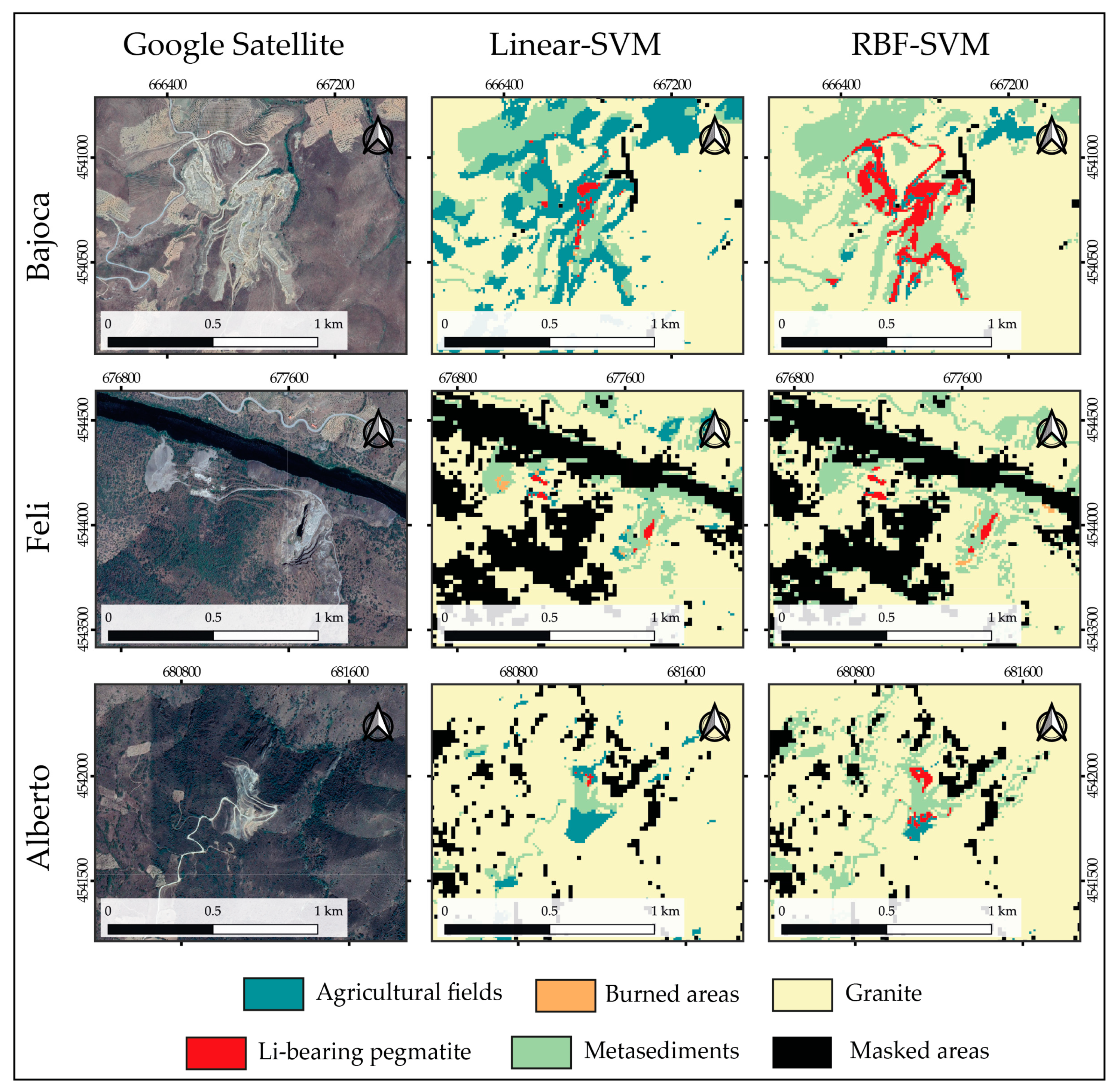
The performance of the models was evaluated in their capacity to correctly identify known target areas. As mentioned before, in the Fregenda–Almendra area there are three open-pit mines currently exploiting Li-bearing pegmatites: the Bajoca mine on the Portuguese side, and the Feli and Alberto mines in Spain. From the 43 Li-pegmatite samples defined for training and evaluation, 42 of those samples belonged to the Bajoca mine (outcropping pegmatite and ore stockpile). The remaining sample was collected from one outcropping pegmatite in the Alberto mine. The classification results obtained for these three target areas using both algorithms are presented in Figure 9.
The results obtained for the Feli mine were similar using the two algorithms, identifying the presence of Li-bearing pegmatite in the open-pit and next to the two waste piles (to the left of the open-pit). However, in the case of the Bajoca and Alberto mines, the Linear-SVM classified a much smaller area as being Li-bearing pegmatite when compared to the RBF model. Oppositely, the RBF-SVM identifies some false positives like in the dirt road that leads to the Bajoca mine (Figure 9). Regarding the other classes, both models overestimated the occurrence of Granite where in fact metasedimentary rocks occur. Moreover, the Linear-SVM misclassified some pixels inside the open-pits as being Agricultural Fields. This misclassification was less frequent with the RBF model.
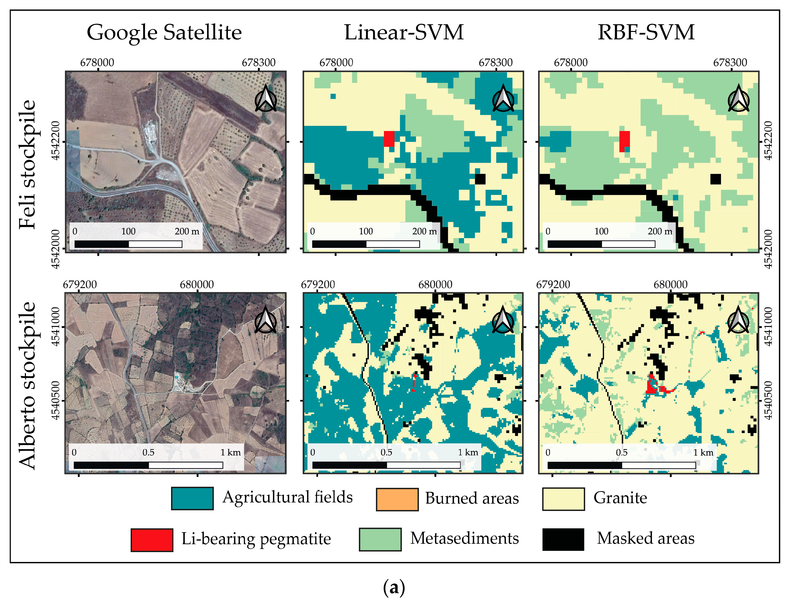
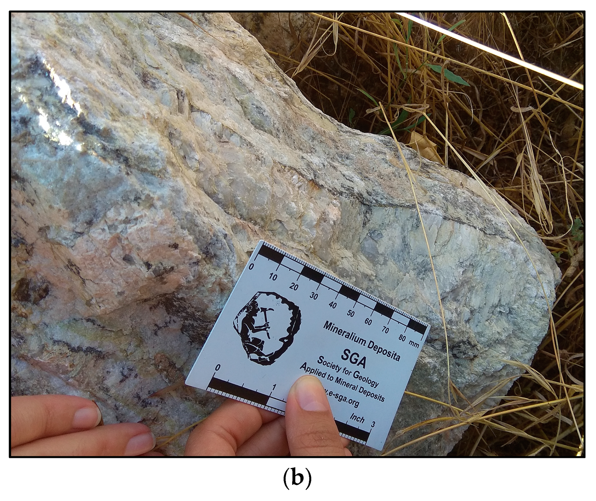
On the contrary to what happens in the Bajoca mine, the ore stockpiles, where the extracted Li-pegmatite from the Feli and Alberto mines are stored, are not located near the open-pits. Therefore, these two known stockpiles were also used to verify the models’ performance in the classification of the Li-bearing pegmatite class (Figure 10). Field campaigns allowed to verify that Li-minerals are present in these stockpiles (Figure 10b). In the case of the Feli stockpile, both models were able to identify the occurrence of Li-bearing pegmatite. Inversely, on the Alberto stockpile, only the RBF-SVM correctly identified most of the areas where Li-pegmatite is present. In what concerns the remaining classes, besides the areas misclassified as Granite, the Linear-SVM was the model that correctly identified most of the Agricultural Fields.
5. Discussion
A previous attempt to use ML algorithms in Li-bearing pegmatite identification showed that the model parameterization and optimization were not enough to avoid overfitting, which ultimately led to a large number of Li-pegmatite false positives [5]. In this study, several methodological improvements were made. Besides reducing the area to be classified and the number of classes through masking of undesired classes, a new strategy to split the training data into training and test subsets was proposed. This new strategy resulted in a higher independency between the two subsets, since sample location was taken into consideration in the split. Inevitably, the random sampling process introduced when using the downsampling and upsampling strategies made the developed ROI-based splitting strategy infeasible. This led to overfitting problems and, therefore, these strategies were excluded from the classification. The proper definition of the range of the tested parameters was crucial to optimize the models during the first stage grid-search, and several literature-based ranges were tested. While several authors have also employed grid-search techniques to determine the best parameter(s) [8,18,19,43,48], this step is not always employed, with some authors achieving parameterization through the trial and error method [14]. Other authors have opted to not optimize the models and used the default parameters or other specific sets of parameters [9,10,12,49]. The observation of the first stage results allowed to select the right parameters, but also to exclude the polynomial kernel, reinforcing the importance of the intervention of the operator at the beginning of the classification process.
The second stage grid-search automatically returned two different models respectively for the imbalanced and balanced datasets, which is the first indication that class imbalance may affect the obtained results. The Linear-SVM trained on the imbalance data and the RBF-SVM trained using the class-weight option showed, at turn, better performance depending on the class. Both models achieved a better ability to discriminate the target class (Li-pegmatite) from the host rocks, thus reducing the number of false positives when compared to the SVM model trained in the previous work of Cardoso-Fernandes, et al. [5]. This corroborates that the methodological adjustments made in the current study helped to improve the SVM performance.
Nonetheless, the results obtained with each model for the Li-bearing pegmatite class were very distinct. The Linear-SVM presented the best discrimination between Li-pegmatite and Metasediments, while missing to correctly classify pixels with known Li-pegmatite exposition. Oppositely, the RBF-SVM avoided the occurrence of Li-pegmatite false negatives while classifying Metasediments and dirt roads as areas with Li-potential. Increasing the discrimination between Metasediments and Li-pegmatites may only be achieved with a better spatial resolution data. In the Fregeneda–Almendra pegmatite field, dyke thickness can range between 4 m and 15 m in the case of the spodumene-bearing dykes, and between 5 m and 30 m in the petalite-bearing ones [25]. Even in the largest dyke that outcrops in the Bajoca mine, metasedimentary enclaves can be found in the middle of the pegmatite, which contributes to pixel mixing, since the Sentinel-2 bands used in this work have between 10 m to 20 m of spatial resolution. In addition, the slightly different mineral paragenesis of the Feli mine (with lepidolite), when compared with Alberto or Bajoca, may have influenced the performance of Linear-SVM.
The interpretations of the final classification maps (Figure 7 and Figure 8) are supported by the computed statistical metrics and respective confusion matrices (Figure A1 and Figure 6). When looking at the performance metrics at a class level, Linear-SVM reached a better performance on the test set (Figure A1), which may indicate more overtraining and fewer ability to generalize to unknown data, when compared with RBF-SVM. When dealing with imbalanced datasets, special attention should be given when interpreting the results obtained with global metrics such as OA and Kappa hat, since the influence that minor classes such as Li-pegmatite have on the final output can be masked by the majority class(es) [44,50]. That is why it is important to qualitatively assess the performance of the models. Zoom images concerning known Li-pegmatite expositions (Figure 9 and Figure 10) support the previous interpretations that the RBF-SVM performs better in Li-pegmatite identification, when compared with the Linear-SVM. Moreover, the results obtained highlight that the developed methodology can identify Li-pegmatite occurrences beyond those that were used as training instances.
In what concerns the remaining lithological classes, both models overestimated the occurrence of Granite in areas where Metasediments occur. This can be mainly explained by the spectral confusion with the Agricultural fields class, especially in the case of the RBF-model. The phenomenon is not only corroborated by the computed confusion matrices, but also by the signature separability measures (see Section 3.1.2.). The overestimation of the Granite class can also be linked to the difficulty to correctly classify the metasedimentary rocks since (i) they outcrop in less extent when compared with the granites, (ii) are often covered by vegetation or (iii) serve for olive/almond tree plantations. This happens because granites are not so easily weathered as the metasediments, and regolith tends to form over the latter. Taking this into account, a regolith–geology mapping approach like the one employed by De Boissieu, et al. [9] could help improve the results.
On the other hand, considering that in geological exploration false negatives should be avoided, the RBF-SVM built using a class balancing strategy is therefore the preferred model to define areas with Li-potential. In satellite image classification, the RBF is often the preferred kernel, commonly showing good performance [12,19,43,49]. Melgani and Bruzzone [51] concluded that the RBF-kernel achieved higher OA than the Linear-model in hyperspectral image classification. Geranian, et al. [16] have compared the performance attained with different kernels in mineral prospectivity mapping and concluded the RBF achieved the best results. However, in a similar study, Zuo and Carranza [13] found the sigmoid kernel to be the optimal function.
Contrary to the expected and opposed to previous studies [5], the results also show that the class imbalance had a higher impact on the SVM performance (Figure 5, Figure 7, Figure 8, Figure 9 and Figure 10). This is of particular interest and importance, since Maxwell, et al. [18] stated that, for SVM, balancing the data had a negligible effect on UA and PA of the rare classes of the Indian pine dataset, Indiana (USA). Noi and Kappas [19] also concluded that SVM was less impacted by sample size and class imbalance than other ML algorithms. However, despite its robustness to data imbalance, the SVM algorithm works by minimizing the overall error (that is inherently biased toward the majority class) which can lead to the underprediction of the less-abundant class [18,50]. In this work, the Li-class was underpredicted using the imbalanced dataset when compared to the balanced one. Ultimately, class imbalance affected the ability to predict the Li-pegmatite class not only in possibly target areas, but also where Li-pegmatite occurrences are known.
Overall, the methodological developments made in this study represent a major contribution not only to the state of the art of Li-pegmatite satellite-based exploration, but also to the application of ML algorithms to remote sensing lithological mapping. The step-by-step optimization made in this study is proof that ML algorithms, particularly SVM, are not easy and ready to apply (at least to some specific applications such as mineral exploration). The major difficulty in Li-pegmatite exploration using remote sensing data is their relatively small size and exposition. This means that, in an image classification problem, the target class is by nature a small, underrepresented class. Therefore, the adaptations proposed to achieve the optimal parameters proved to be fundamental to successfully deal with class imbalance. Detailed insights on algorithm parameterization were given, so that the methodology can be replicated in other case studies. Algorithm optimization was reached at several levels, namely: (i) data splitting for training and testing; (ii) strategy do deal with data imbalance; (iii) type of SVM model and kernel function; (iv) associated hyperparameter(es); and (v) metric score employed in the CV process. When using a grid-search with CV to find the best parameters, commonly used metrics are the OA and Kappa statistics [8,18,19]. As part of the algorithm optimization, a more innovative strategy was employed in the first stage grid-search where the parameters were chosen based on the F1-score of just two classes: the Li-pegmatite and the Metasediments. Moreover, the semi-automatization of the SVM classification process allowed to simplify the choice of the best model among several options. In this case, the results obtained with the RBF-SVM allowed to delineate target areas for Li-exploration.
However, the developed methodology still has some shortcomings. The main limitation is that some smaller pegmatite occurrences and other potential areas for Li-exploration were missed while trying to increase the discrimination between the Li-pegmatite class and the Metasediments. This can be related or accentuated by the low ratio between pegmatite size and the satellite image spatial resolution. This issue was vastly explained in previous studies [7,32]. Another major concern in ML and deep learning (DL) remote sensing applications is the ability to transfer learning between case studies [52]. Unfortunately, there is no current solution for this problem, but in this study, we wanted to ensure that the improved methodology and SVM optimization could be applied to other datasets and study areas. To achieve this goal, the first stage grid-search was optimized to discriminate the target area from the host-rocks. Thus, when applying to another area, the operator should adapt the source code available in Section 2 of Supplementary Materials, to create a personalized metric score concerning the Li-bearing pegmatite and the existing host-rocks. In this metric score, a beta coefficient can be added to the F1-score, thus creating an F-beta score that allows the operator to adjust the relative importance of precision and recall, according to characteristics of the study area.
6. Conclusions
In this study, untraditional approaches were developed and employed to improve SVM performance in Li-pegmatite mapping. Several kernelized and non-kernelized SVM’s models with different parameter ranges were trained to find the optimal model. Overall, the objectives of this work were accomplished, and the research questions proposed were addressed with the new methodological advances proposed:
- To overcome and avoid overfitting, a new splitting strategy based on the regions of interest (ROIs) was developed and applied with success to create the training and test subsets.
- The choice of an adequate metric score proved to be essential not only in the parameter optimization but also in the model evaluation step. To maximize the discrimination between the target (Li-pegmatites) and the host rocks, a customized metric score was created for the first stage grid-search with CV.
- A semi-automatized process allowed to choose the best model among several options. However, a blind automatization of the SVM classification is not yet possible, since the intervention of the operator is fundamental at the beginning of the model training and parameterization.
- The methodological adjustments proposed in this study improved the previously obtained results with SVM for the same study area, by reducing model overfitting and improving the discrimination between Li-pegmatites and their host-rock. The best model found with the semi-automatized process was the one built with the RBF kernel and using the class-weight option to account for imbalanced data.
- Contrary to the results obtained by other authors, this study shows that the class imbalance had a negative impact on the SVM performance, and the adaptations made to account for the imbalanced nature of the data were crucial for successfully delineating Li-pegmatite occurrences.
- On the other hand, the qualitative assessment of the SVM models’ performance highlighted the success and potential of the methodology in the identification of known Li-pegmatite occurrences beyond those used for training. Other target areas for Li-exploration were also delineated using the RBF-SVM model.
- The main limitation found was that some smaller pegmatite occurrences and other potential areas for Li-exploration were missed while trying to optimize class separability and reduce overfitting. Therefore, the right balance between increasing the separability of Li-pegmatite/host-rocks and minimizing false negatives needs to be found. This can be achieved with higher resolution satellite images. Different ML algorithms can also be compared.
- Furthermore, the methodological optimization made in this study already provides tools to personalize and help generalize its application to other locations. This approach could also be modified to map remotely other types of pegmatites containing important mineral commodities like rare elements and gemstones.
Despite the encountered limitations, these results still represent a major contribution to the state of art regarding the use of ML in Li-pegmatite mapping. Moreover, the newly developed methodological approach can be very helpful for the exploration/mining industry, since the ability to remotely map mineralized pegmatites can reduce the costs of exploration campaigns while increasing the social acceptance of mineral exploration through the use of more conscientious environmental practices.
Supplementary Materials
The source code developed in this study is available online at https://www.mdpi.com/2072-4292/12/14/2319/s1, Section 1: Splitting the data into training and test subsets; Section 2: First stage grid-search; Section 3: Second stage grid-search, model evaluation and image prediction.
Author Contributions
All the authors conceived and designed the experiments; J.C.-F. performed the experiments and conducted the research; all the authors analyzed the data; J.C.-F. wrote the paper; A.C.T., A.L., and E.R.-R. revised the paper. All authors have read and agreed to the published version of the manuscript.
Funding
The authors would like to thank the financial support provided by FCT—Fundação para a Ciência e a Tecnologia, I.P., with the ERA-MIN/0001/2017—LIGHTS project. The work was also supported by National Funds through the FCT project UIDB/04683/2020—ICT (Institute of Earth Sciences). Joana Cardoso-Fernandes is financially supported within the compass of a Ph.D. Thesis, ref. SFRH/BD/136108/2018, by national funds from MCTES through FCT, and co-financed by the European Social Fund (ESF) through POCH—Programa Operacional Capital Humano. The Spanish Ministerio de Ciencia, Innovacion y Universidades (Project RTI2018-094097-B-100, with ERDF funds) and the University of the Basque Country (UPV/EHU) (grant GIU18/084) also contributed economically.
Acknowledgments
The authors would like to thank N. Pires (University of Porto) for helping with Python coding.
Conflicts of Interest
The authors declare no conflict of interest. The funders had no role in the design of the study; in the collection, analyses, or interpretation of data; in the writing of the manuscript, or in the decision to publish the results.
Appendix A
Figure A1.
Confusion matrix for the Linear-SVM model built on the imbalanced dataset.

References
- Cardoso-Fernandes, J.; Teodoro, A.C.; Lima, A. Potential of Sentinel-2 data in the detection of lithium (Li)-bearing pegmatites: A study case. In Proceedings of the SPIE Remote Sensing, Berlin, Germany, 10–13 September 2018; p. 15. [Google Scholar]
- Cardoso-Fernandes, J.; Teodoro, A.C.; Lima, A. Remote sensing data in lithium (Li) exploration: A new approach for the detection of Li-bearing pegmatites. Int. J. Appl. Earth Obs. Geoinf. 2019, 76, 10–25. [Google Scholar] [CrossRef]
- Perrotta, M.M.; Souza Filho, C.R.; Leite, C.A.S. Mapeamento espectral de intrusões pegmatíticas relacionadas a mineralizações de lítio, gemas e minerais industriais na região do vale do Jequitinhonha (MG) a partir de imagens ASTER. In Proceedings of the Anais do XII Simpósio Brasileiro de Sensoriamento Remoto, Goiânia, Brazil, 16–21 April 2005; pp. 1855–1862. [Google Scholar]
- Mendes, D.; Perrotta, M.M.; Costa, M.A.C.; Paes, V.J.C. Mapeamento espectral para identificação de assinaturas espectrais de minerais de lítio em imagens ASTER (NE/MG). In Proceedings of the Anais do XVIII Simpósio Brasileiro de Sensoriamento Remoto, Santos-SP, Brazil, 28–29 May 2017; pp. 5273–5280. [Google Scholar]
- Cardoso-Fernandes, J.; Teodoro, A.C.; Lima, A.; Roda-Robles, E. Evaluating the performance of support vector machines (SVMs) and random forest (RF) in Li-pegmatite mapping: Preliminary results. In Proceedings of the SPIE Remote Sensing, Strasbourg, France, 9–12 September 2019. [Google Scholar]
- Santos, D.; Teodoro, A.; Lima, A.; Cardoso-Fernandes, J. Remote sensing techniques to detect areas with potential for lithium exploration in Minas Gerais, Brazil. In Proceedings of the SPIE Remote Sensing, Strasbourg, France, 9–12 September 2019. [Google Scholar]
- Cardoso-Fernandes, J.; Teodoro, A.C.; Lima, A.; Perrotta, M.; Roda-Robles, E. Detecting Lithium (Li) Mineralizations from Space: Current Research and Future Perspectives. Appl. Sci. 2020, 10, 1785. [Google Scholar] [CrossRef] [Green Version]
- Yu, L.; Porwal, A.; Holden, E.-J.; Dentith, M.C. Towards automatic lithological classification from remote sensing data using support vector machines. Comput. Geosci. 2012, 45, 229–239. [Google Scholar] [CrossRef]
- De Boissieu, F.; Sevin, B.; Cudahy, T.; Mangeas, M.; Chevrel, S.; Ong, C.; Rodger, A.; Maurizot, P.; Laukamp, C.; Lau, I.; et al. Regolith-geology mapping with support vector machine: A case study over weathered Ni-bearing peridotites, New Caledonia. Int. J. Appl. Earth Obs. Geoinf. 2018, 64, 377–385. [Google Scholar] [CrossRef]
- Othman, A.A.; Gloaguen, R. Improving Lithological Mapping by SVM Classification of Spectral and Morphological Features: The Discovery of a New Chromite Body in the Mawat Ophiolite Complex (Kurdistan, NE Iraq). Remote Sens. 2014, 6, 6867–6896. [Google Scholar] [CrossRef] [Green Version]
- Latifovic, R.; Pouliot, D.; Campbell, J. Assessment of Convolution Neural Networks for Surficial Geology Mapping in the South Rae Geological Region, Northwest Territories, Canada. Remote Sens. 2018, 10, 307. [Google Scholar] [CrossRef] [Green Version]
- Gasmi, A.; Gomez, C.; Zouari, H.; Masse, A.; Ducrot, D. PCA and SVM as geo-computational methods for geological mapping in the southern of Tunisia, using ASTER remote sensing data set. Arab. J. Geosci. 2016, 9, 753. [Google Scholar] [CrossRef]
- Zuo, R.; Carranza, E.J.M. Support vector machine: A tool for mapping mineral prospectivity. Comput. Geosci. 2011, 37, 1967–1975. [Google Scholar] [CrossRef]
- Abedi, M.; Norouzi, G.-H.; Bahroudi, A. Support vector machine for multi-classification of mineral prospectivity areas. Comput. Geosci. 2012, 46, 272–283. [Google Scholar] [CrossRef]
- Rodriguez-Galiano, V.; Sanchez-Castillo, M.; Chica-Olmo, M.; Chica-Rivas, M. Machine learning predictive models for mineral prospectivity: An evaluation of neural networks, random forest, regression trees and support vector machines. Ore Geol. Rev. 2015, 71, 804–818. [Google Scholar] [CrossRef]
- Geranian, H.; Tabatabaei, S.H.; Asadi, H.H.; Carranza, E.J.M. Application of Discriminant Analysis and Support Vector Machine in Mapping Gold Potential Areas for Further Drilling in the Sari-Gunay Gold Deposit, NW Iran. Nat. Resour. Res. 2016, 25, 145–159. [Google Scholar] [CrossRef]
- Mountrakis, G.; Im, J.; Ogole, C. Support vector machines in remote sensing: A review. ISPRS J. Photogramm. Remote Sens. 2011, 66, 247–259. [Google Scholar] [CrossRef]
- Maxwell, A.E.; Warner, T.A.; Fang, F. Implementation of machine-learning classification in remote sensing: An applied review. Int. J. Remote Sens. 2018, 39, 2784–2817. [Google Scholar] [CrossRef] [Green Version]
- Noi, P.T.; Kappas, M. Comparison of Random Forest, k-Nearest Neighbor, and Support Vector Machine Classifiers for Land Cover Classification Using Sentinel-2 Imagery. Sensors 2017, 18, 18. [Google Scholar] [CrossRef] [Green Version]
- Roda, E. Distribución, Caracteristicas y Petrogenesis de las Pegmatitas de La Fregeneda (Salamanca). Ph.D. Thesis, UPV/EHU, Bilbao, Spain, 1993. [Google Scholar]
- Roda-Robles, E.; Pesquera, A.; Velasco, F.; Fontan, F. The granitic pegmatites of the Fregeneda area (Salamanca, Spain): Characteristics and petrogenesis. Miner. Mag. 1999, 63, 535–558. [Google Scholar] [CrossRef]
- Vieira, R. Aplitopegmatitos com elementos raros da região entre Almendra (V.N. de Foz Côa) e Barca d’Alva (Figueira de Castelo Rodrigo). Campo aplitopegmatítico da Fregeneda- Almendra. Ph.D. Thesis, Faculdade de Ciências da Universidade do Porto, Porto, Portugal, 2010. [Google Scholar]
- Costa, J.C.S.D. Notícia sobre uma carta geológica do Buçaco, de Nery Delgado; Serviços Geológicos de Portugal: Lisboa, Portugal, 1950. [Google Scholar]
- Teixeira, C. Notas sobre geologia de Portugal o complexo xisto-grauváquico ante-ordoviciano; Empresa Literaria Fluminense Lda.: Lisboa, Portugal, 1955; p. 48. [Google Scholar]
- Roda-Robles, E.; Vieira, R.; Pesquera, A.; Lima, A. Chemical variations and significance of phosphates from the Fregeneda-Almendra pegmatite field, Central Iberian Zone (Spain and Portugal). Miner. Pet. 2010, 100, 23–34. [Google Scholar] [CrossRef]
- Silva, A.F.d.; Rebelo, J.A.; Ribeiro, M.L. Notícia Explicativa da folha 11-C Torre de Moncorvo; Serviços Geológicos de Portugal: Lisboa, Portugal, 1989; p. 65. [Google Scholar]
- Silva, A.F.d.; Ribeiro, M.L. Notícia Explicativa da folha 15-A Vila Nova de Foz Côa; Serviços Geológicos de Portugal: Lisboa, Portugal, 1991; p. 52. [Google Scholar]
- Vapnik, V.N. The Nature of Statistical Learning Theory; Springer: New York, NY, USA, 1995. [Google Scholar]
- Knerr, S.; Personnaz, L.; Dreyfus, G. Single-layer learning revisited: A stepwise procedure for building and training a neural network. In Neurocomputing; Soulié, F.F., Hérault, J., Eds.; Springer: Berlin/Heidelberg, Germany, 1990; pp. 41–50. [Google Scholar]
- Cortes, C.; Vapnik, V. Support-vector networks. Mach. Learn. 1995, 20, 273–297. [Google Scholar] [CrossRef]
- Géron, A. Hands-On Machine Learning with Scikit-Learn and TensorFlow: Concepts, Tools, and Techniques to Build Intelligent Systems; O’Reilly Media, Inc.: Sebastopol, CA, USA, 2017; p. 568. [Google Scholar]
- Cardoso-Fernandes, J.; Lima, A.; Roda-Robles, E.; Teodoro, A.C. Constraints and potentials of remote sensing data/techniques applied to lithium (Li)-pegmatites. Can. Miner. 2019, 57, 723–725. [Google Scholar] [CrossRef]
- Missions: Sentinel-2. Available online: https://sentinel.esa.int/web/sentinel/missions/sentinel-2 (accessed on 20 April 2020).
- MultiSpectral Instrument (MSI) Overview. Available online: https://sentinel.esa.int/web/sentinel/technical-guides/sentinel-2-msi/msi-instrument (accessed on 20 April 2020).
- Sentinel-2 MSI: Products and Algorithms. Available online: https://sentinel.esa.int/web/sentinel/technical-guides/sentinel-2-msi/products-algorithms (accessed on 20 April 2020).
- SNAP. Available online: https://step.esa.int/main/toolboxes/snap/ (accessed on 20 April 2020).
- Google Earth Pro. Available online: https://www.google.com/intl/en_uk/earth/desktop/ (accessed on 3 August 2018).
- Esri World Imagery. Available online: https://www.arcgis.com/home/item.html?id=10df2279f9684e4a9f6a7f08febac2a9 (accessed on 9 May 2019).
- Geomatica 2018. Available online: https://www.pcigeomatics.com/ (accessed on 12 July 2019).
- Geomatica Help. Available online: http://www.pcigeomatics.com/geomatica-help/ (accessed on 23 April 2019).
- Pedregosa, F.; Varoquaux, G.; Gramfort, A.; Michel, V.; Thirion, B.; Grisel, O.; Blondel, M.; Prettenhofer, P.; Weiss, R.; Dubourg, V.; et al. Scikit-learn: Machine Learning in Python. J. Mach. Learn. Res. 2012, 12, 2825–2830. [Google Scholar]
- 1.4. Support Vector Machines—Scikit-Learn 0.20.4 Documentation. Available online: https://scikit-learn.org/0.20/modules/svm.html#svm-classification (accessed on 24 April 2020).
- Oommen, T.; Misra, D.; Twarakavi, N.K.C.; Prakash, A.; Sahoo, B.; Bandopadhyay, S. An Objective Analysis of Support Vector Machine Based Classification for Remote Sensing. Math. Geosci. 2008, 40, 409–424. [Google Scholar] [CrossRef]
- Müller, A.C.; Guido, S. Chapter 5. Model Evaluation and Improvement. In Introduction to Machine Learning with Python: A Guide for Data Scientists; Schanafelt, D., Ed.; O’Reilly Media, Inc.: Sebastopol, CA, USA, 2016; pp. 251–303. [Google Scholar]
- Story, M.; Congalton, R. Accuracy assessment: A user’s perspective. Photogramm. Eng. Remote Sens. 1986, 52, 397–399. [Google Scholar]
- Congalton, R.G. A review of assessing the accuracy of classifications of remotely sensed data. Remote Sens. Environ. 1991, 37, 35–46. [Google Scholar] [CrossRef]
- Cohen, J. A Coefficient of Agreement for Nominal Scales. Educ. Psychol. Meas. 1960, 20, 37–46. [Google Scholar] [CrossRef]
- Cracknell, M.J.; Reading, A.M.; McNeill, A.W. Mapping geology and volcanic-hosted massive sulfide alteration in the Hellyer–Mt Charter region, Tasmania, using Random Forests™ and Self-Organising Maps. Aust. J. Earth Sci. 2014, 61, 287–304. [Google Scholar] [CrossRef]
- Pal, M.; Mather, P.M. Support vector machines for classification in remote sensing. Int. J. Remote Sens. 2005, 26, 1007–1011. [Google Scholar] [CrossRef]
- He, H.; Garcia, E.A. Learning from Imbalanced Data. IEEE Trans. Knowl. Data Eng. 2009, 21, 1263–1284. [Google Scholar] [CrossRef]
- Melgani, F.; Bruzzone, L. Classification of hyperspectral remote sensing images with support vector machines. IEEE Trans. Geosci. Remote Sens. 2004, 42, 1778–1790. [Google Scholar] [CrossRef] [Green Version]
- Li, Y.; Zhang, H.; Xue, X.; Jiang, Y.; Shen, Q. Deep learning for remote sensing image classification: A survey. Wiley Interdiscip. Rev. Data Min. Knowl. Discov. 2018, 8, e1264. [Google Scholar] [CrossRef] [Green Version]
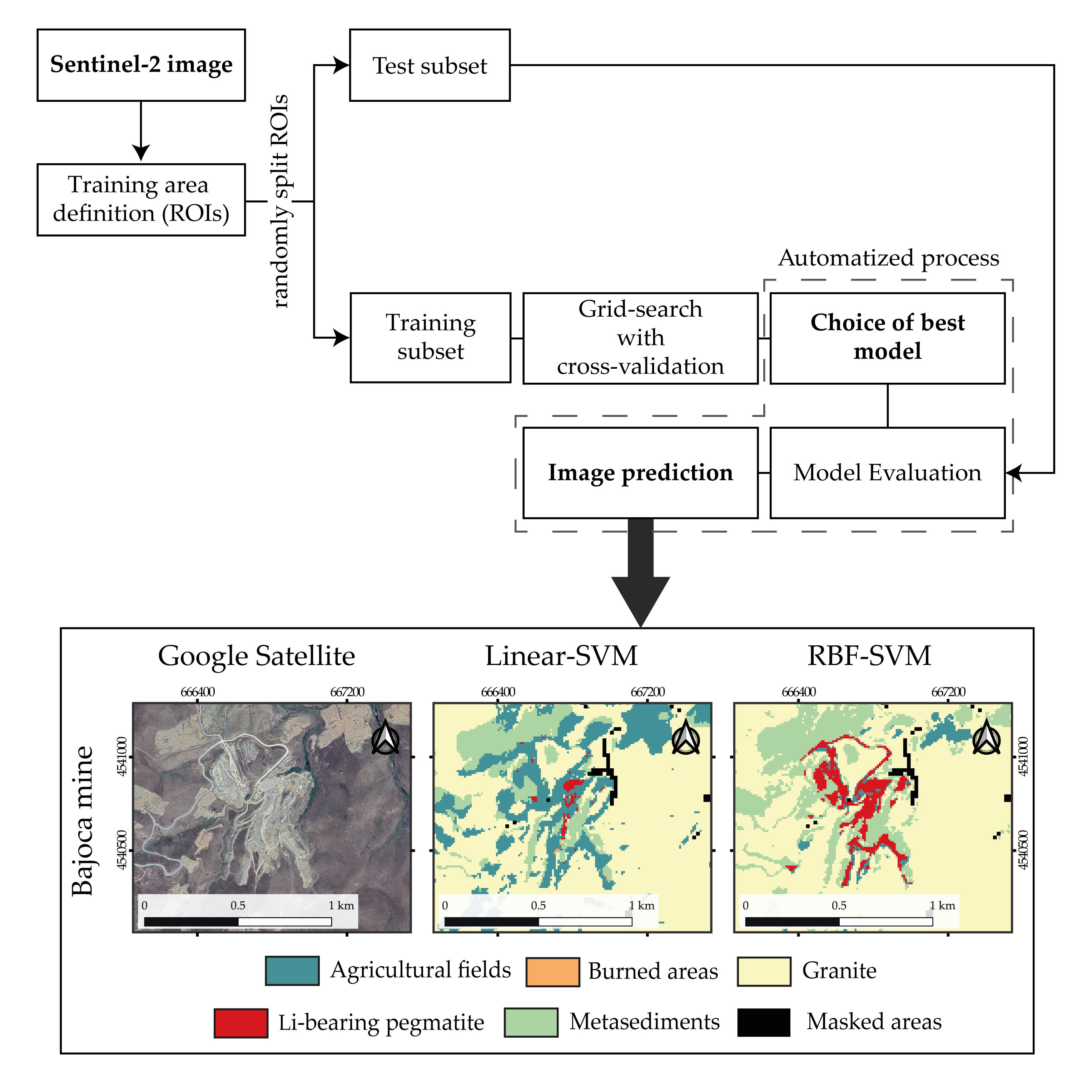
Figure 1.
Location and geological map of the study area where the different aplite–pegmatite dykes outcrop (adapted from [22,26,27]). Open-pit mines of Bajoca, Feli and Alberto are also highlighted. The map projection is Universal Transverse Mercator zone 29 N from the WGS84 datum.

Figure 2.
The support vector machines (SVM) method: the optimal hyperplane separates the two classes and is parallel to the bounding hyperplanes on which the support vectors lie. The distance between these two bounding hyperplanes is called the margin, and the distance d between the bounding hyperplane and the outlier (misclassified sample) indicates that there are slack variables (modified from [8]).

Figure 3.
Mean spectral signatures based on the training pixels selected for each class.

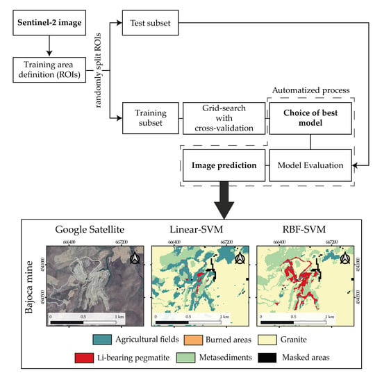
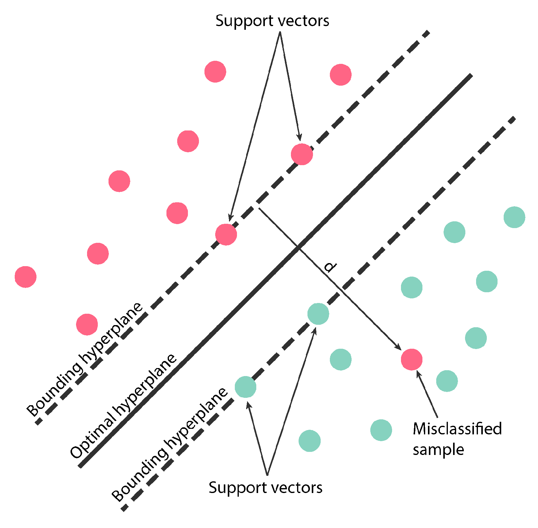
Figure 4.
Flowchart of the image classification process.

Figure 5.
Receiver operating characteristic (ROC) curves and area under the curve (AUC) scores for each of the models tested in the second stage grid-search for both the imbalanced and balanced data.
Figure 5.
Receiver operating characteristic (ROC) curves and area under the curve (AUC) scores for each of the models tested in the second stage grid-search for both the imbalanced and balanced data.

Figure 6.
Confusion matrix for the RBF-SVM model built on the balanced dataset.

Figure 7.
Final classification map based on the Linear-SVM model built with imbalanced data. Three open-pit mines exploiting Li-minerals are identified: A—Bajoca, B—Feli, and C—Alberto. The dashed purple line represents the simplified contact between the Metasediments and the Granite. Zoom images of the open-pit mines can be found in Figure 9.

Figure 8.
Final classification map based on the RBF-SVM model built with the balanced data. A—Bajoca mine, B—Feli mine, and C—Alberto mine. Dashed purple line: simplified contact between the Metasediments and the Granite. Zoom images of the open-pit mines can be found in Figure 9.
Figure 8.
Final classification map based on the RBF-SVM model built with the balanced data. A—Bajoca mine, B—Feli mine, and C—Alberto mine. Dashed purple line: simplified contact between the Metasediments and the Granite. Zoom images of the open-pit mines can be found in Figure 9.

Figure 9.
Evaluation of the models’ performance in the known open-pit mines exploiting Li-bearing pegmatite.
Figure 9.
Evaluation of the models’ performance in the known open-pit mines exploiting Li-bearing pegmatite.

Figure 10.
Evaluation of the models’ performance in known ore stockpiles containing Li-bearing minerals (a). (b) Field photograph of a spodumene crystal (a Li-bearing mineral) from the Alberto stockpile.
Figure 10.
Evaluation of the models’ performance in known ore stockpiles containing Li-bearing minerals (a). (b) Field photograph of a spodumene crystal (a Li-bearing mineral) from the Alberto stockpile.


Table 1.
Sentinel-2B Band’s Characteristics [34].
Table 1.
Sentinel-2B Band’s Characteristics [34].
| Band Number | Central Wavelength (nm) | Bandwidth (nm) | Spatial Resolution (m) |
|---|---|---|---|
| 1 | 442.3 | 21 | 60 |
| 2 | 492.1 | 66 | 10 |
| 3 | 559.0 | 36 | 10 |
| 4 | 665.0 | 31 | 10 |
| 5 | 703.8 | 16 | 20 |
| 6 | 739.1 | 15 | 20 |
| 7 | 779.7 | 20 | 20 |
| 8 | 833.0 | 106 | 10 |
| 8A | 864.0 | 22 | 20 |
| 9 | 943.2 | 21 | 60 |
| 10 | 1376.9 | 30 | 60 |
| 11 | 1610.4 | 94 | 20 |
| 12 | 2185.7 | 185 | 20 |
Table 2.
Distribution of Training Pixels by Classes and regions of interest (ROIs).
| Class name | Total Pixel Number | Training Pixels | Testing Pixels | ROI Number |
|---|---|---|---|---|
| Agricultural fields | 1230 | 894 | 336 | 8 |
| Burned areas | 205 | 80 | 125 | 2 |
| Granite | 1231 | 987 | 244 | 9 |
| Li-bearing pegmatite | 43 | 17 | 26 | 5 |
| Metasediments | 344 | 166 | 178 | 9 |
Table 3.
Jeffries–Matusita (JM) (Blue) and transformed divergence (TD) (Orange) Separability Measures for Each Pair of Classes.
Table 3.
Jeffries–Matusita (JM) (Blue) and transformed divergence (TD) (Orange) Separability Measures for Each Pair of Classes.
| Li-Bearing Pegmatite | Metasediments | Granite | Burned Areas | Agricultural Fields | |
|---|---|---|---|---|---|
| Li-bearing pegmatite | 2.000 | 2.000 | 2.000 | 2.000 | |
| Metasediments | 1.977 | 2.000 | 2.000 | 2.000 | |
| Granite | 2.000 | 1.998 | 2.000 | 1.994 | |
| Burned areas | 2.000 | 2.000 | 2.000 | 2.000 | |
| Agricultural fields | 1.998 | 1.994 | 1.865 | 2.000 |
Table 4.
Classification Performance Summary for the Two Models Built.
| Model | Imbalanced | Balanced | |
|---|---|---|---|
| Linear Model | RBF Kernel | ||
| Parameter(s) | C = 32 | C = 0.2 | γ = 4.4 |
| Mean train score (CV) | 0.980643 | 0.941802 | |
| Mean test score (CV) | 0.917444 | 0.93750 | |
| Overall accuracy (OA) | 0.852585 | 0.832783 | |
| Kappa hat | 0.801678 | 0.777337 | |
| Nested CV score | 0.906241 | 0.906229 | |
Table 5.
User’s and producer’s accuracy (UA and PA) for Both the Linear-SVM and Radial Basis Function (RBF)-SVM Models. Values in percentage (%).
Table 5.
User’s and producer’s accuracy (UA and PA) for Both the Linear-SVM and Radial Basis Function (RBF)-SVM Models. Values in percentage (%).
| Class | Imbalanced | Balanced | ||
|---|---|---|---|---|
| PA | UA | PA | UA | |
| Agricultural fields | 64.58 | 93.53 | 61.01 | 99.51 |
| Burned areas | 100.00 | 100.00 | 100.00 | 100.00 |
| Granite | 98.77 | 66.94 | 100.00 | 65.07 |
| Li-bearing pegmatite | 88.46 | 100.00 | 96.15 | 59.52 |
| Metasediments | 94.94 | 100.00 | 90.45 | 100.00 |
© 2020 by the authors. Licensee MDPI, Basel, Switzerland. This article is an open access article distributed under the terms and conditions of the Creative Commons Attribution (CC BY) license (http://creativecommons.org/licenses/by/4.0/).
Share and Cite
MDPI and ACS Style
Cardoso-Fernandes, J.; Teodoro, A.C.; Lima, A.; Roda-Robles, E. Semi-Automatization of Support Vector Machines to Map Lithium (Li) Bearing Pegmatites. Remote Sens. 2020, 12, 2319. https://doi.org/10.3390/rs12142319
AMA Style
Cardoso-Fernandes J, Teodoro AC, Lima A, Roda-Robles E. Semi-Automatization of Support Vector Machines to Map Lithium (Li) Bearing Pegmatites. Remote Sensing. 2020; 12(14):2319. https://doi.org/10.3390/rs12142319
Chicago/Turabian StyleCardoso-Fernandes, Joana, Ana C. Teodoro, Alexandre Lima, and Encarnación Roda-Robles. 2020. "Semi-Automatization of Support Vector Machines to Map Lithium (Li) Bearing Pegmatites" Remote Sensing 12, no. 14: 2319. https://doi.org/10.3390/rs12142319
Note that from the first issue of 2016, this journal uses article numbers instead of page numbers. See further details here.