Creating New Near-Surface Air Temperature Datasets to Understand Elevation-Dependent Warming in the Tibetan Plateau

Abstract

The Tibetan Plateau has been undergoing accelerated warming over recent decades, and is considered an indicator for broader global warming phenomena. However, our understanding of warming rates with elevation in complex mountain regions is incomplete. The most serious concern is the lack of high-quality near-surface air temperature (Tair) datasets in these areas. To address this knowledge gap, we developed an automated mapping framework for the estimation of seamless daily minimum and maximum Land Surface Temperatures (LSTs) for the Tibetan Plateau from the existing MODIS LST products for a long period of time (i.e., 2002–present). Specific machine learning methods were developed and linked with target-oriented validation and then applied to convert LST to Tair. Spatial variables in retrieving Tair, such as solar radiation and vegetation indices, were used in estimation of Tair, whereas MODIS LST products were mainly focused on temporal variation in surface air temperature. We validated our process using independent Tair products, revealing more reliable estimates on Tair; the R² and RMSE at monthly scales generally fell in the range of 0.9–0.95 and 1–2 °C. Using these continuous and consistent Tair datasets, we found temperature increases in the elevation range between 2000–3000 m and 4000–5000 m, whereas the elevation interval at 6000–7000 m exhibits a cooling trend. The developed datasets, findings and methodology contribute to global studies on accelerated warming.

1. Introduction

The Tibetan Plateau (TP) is named "the third pole of the Earth", and is the highest and largest plateau in the world [1]. The TP exerts profound dynamic and thermal influences on the regional and global climate [2,3]. For global warming, the TP is considered an early warning sign. Over the period of 1984–2009, TP has undergone serious warming, with a warming rate of 0.46 °C per decade⁻¹, which is almost 1.5 times the rate of global warming [4,5]. Accelerated warming on the TP has intensified permafrost degradation, snow melt and glacier retreat [6]. Presently, the status of TP warming is evaluated through the analysis of Tair at meteorological stations. However, most meteorological stations are located in the eastern TP below 3800 m. Because of sparse high-elevation meteorological observations in central and northwest TP, there is a possibility that we may not capture the greatest warming rate over some regions [7]. In addition to limited coverage by in situ measurements, Tair at TP suffers from extreme local variability due to factors such as topography and exposure [8]. Therefore, improved Tair estimations by developing high-resolution products considering the rugged terrain in the TP is a crucial step for understanding the accelerated warming occurring there.

Remotely sensed Land Surface Temperature (LST) is a crucial parameter in the modelling of the surface energy balance at regional and global scales [9,10,11]. LST also provides the possibility of getting high spatial-temporal daily Tair datasets (Tair). Since the late 1980s, a variety of long-time series LST products from Moderate Resolution Imaging Spectroradiometer (MODIS), Advanced Along-Track Scanning Radiometer (AATSR), Advanced Spaceborne Thermal Emission and Reflection Radiometer (ASTER), Multi-Functional Transport Satellite (MTSAT), and Geostationary Operational Environment Satellite have been published [12]. MODIS Terra/Aqua sensors provide close temporal proximity of overpasses, with four LST datasets per day. Many studies have focused on using various combinations of the four MODIS LST datasets to estimate Tair [13,14,15]. Studies have also investigated how to combine the four LST datasets to create composite daily minimum and maximum LST values that supplement the existing Terra/Aqua LST products and reduce areas of missing data. Crosson and Al-Hamdan [16] increased the data coverage of MODIS LST in the United States by 24% and 30% for daily minimum and maximum LST, respectively. Li and Zhou [17] developed a hybrid gap-filling method that merged datasets from existing LST products to fill gaps while integrating with a spatio-temporal gap-filling method to fill the rest of MODIS daily LST gaps, finally creating LSTs dataset over the urban and surrounding areas of United States. However, to the best of our knowledge, no attempt has been made to explore an automated mapping framework for the estimation of daily seamless minimum and maximum LSTs from the four MODIS LST products.

LST is not equivalent to Tair, and their relationship is complex from a theoretical and empirical perspective [14]. Hence, it is difficult to estimate surface air temperature solely using LST, and additional auxiliary factors are used to estimate the Tair in mountainous regions using three representative methods. (1) A semi-empirical method which builds a linear relationship between MODIS LST and a vegetation index, such that Tair can be extrapolated by allowing the regression line to intersect with the vegetation index of full cover [18,19]. (2) A spatio-temporal regression method is used, such as a geographically and temporally weighted regression (GWTR) or a regression-kriging method, both of which consider the relationship between Tair and other variables such as MODIS LST and topographical layers [20,21]. (3) Machine learning models predict Tair from multiple data sources including LST, whilst considering spatio-temporal autocorrelation of Tair [15,22]. In general, each method has been proven to be successful in estimating Tair, but they still have shortcomings in large-scale complex mountainous areas with limited weather stations. For example, the Temperature-Vegetation Index (TVX) method is not appropriate for estimating Tair in regions with low vegetation cover [23]. Statistical models fail to capture the nonlinear behaviour of the climate system in mountainous area. Machine learning models, such as Random Forest, Cubist and Support Vector Machine (SVM), have proven to be flexible in areas with complex terrains like the TP for estimating Tair from LST and additional variables [23]. But they require more datasets for model training. The problem is that training datasets is usually insufficient in such complex mountainous areas. In addition, machine learning models often fail to capture the extreme low and high values of Tair [24,25]. Furthermore, the estimated performance of machine learning models risks spatio-temporal overfitting, which partly depends on different validation strategies [26]. Thus, further investigated is required to identify the accuracy and performance of machine learning models in the absence of sufficient field observations in the complex mountainous areas of TP.

Other environmental datasets, such as vegetation indices, snow cover, albedo, soil type and water bodies, are highly related to Tair. LST with such auxiliary information enables the estimation of Tair within mountainous areas using machine learning models. It is well known that the variation of incoming solar radiation has a strong relationship with the spatial temporal dynamic of Tair [27]. In previous studies, solar zenith and sunshine duration were used as substitutes for mountainous solar radiation for Tair estimation [15]. In this study, we will incorporate truly mountainous solar radiation datasets as one of the covariates for Tair estimation [28]. We assumed that solar radiation and biophysical factors would be related to spatial variability in Tair, whereas we predicted that MODIS LST would be more strongly related to temporal variation in Tair.

The objectives of this study were to (1) create seamless 1000 m daily MODIS LST datasets using a hybrid method; (2) predict Tair using LST and remotely sensed indices with machine learning; (3) compare the performance of different machine learning methods for estimating maximum, minimum and mean air temperature accordingly; and (4) explore elevation-dependent warming over the TP using decadal temperature datasets.

2. Materials and Methods

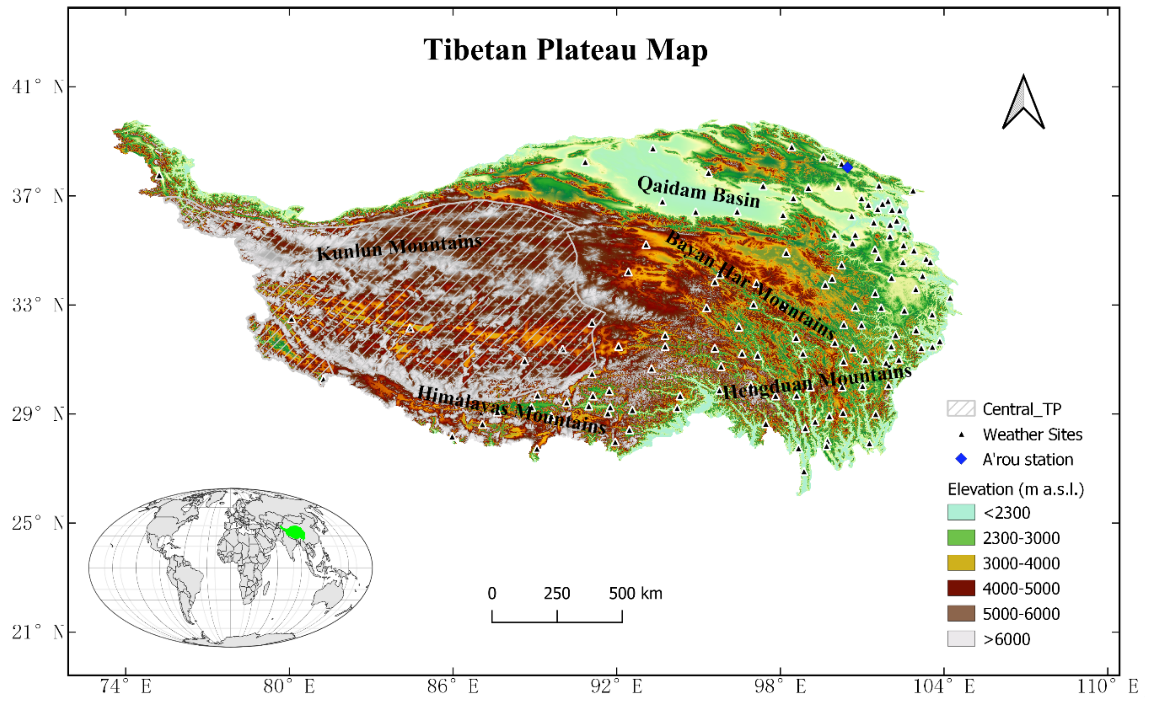
2.1. Study Area and All Climate Data

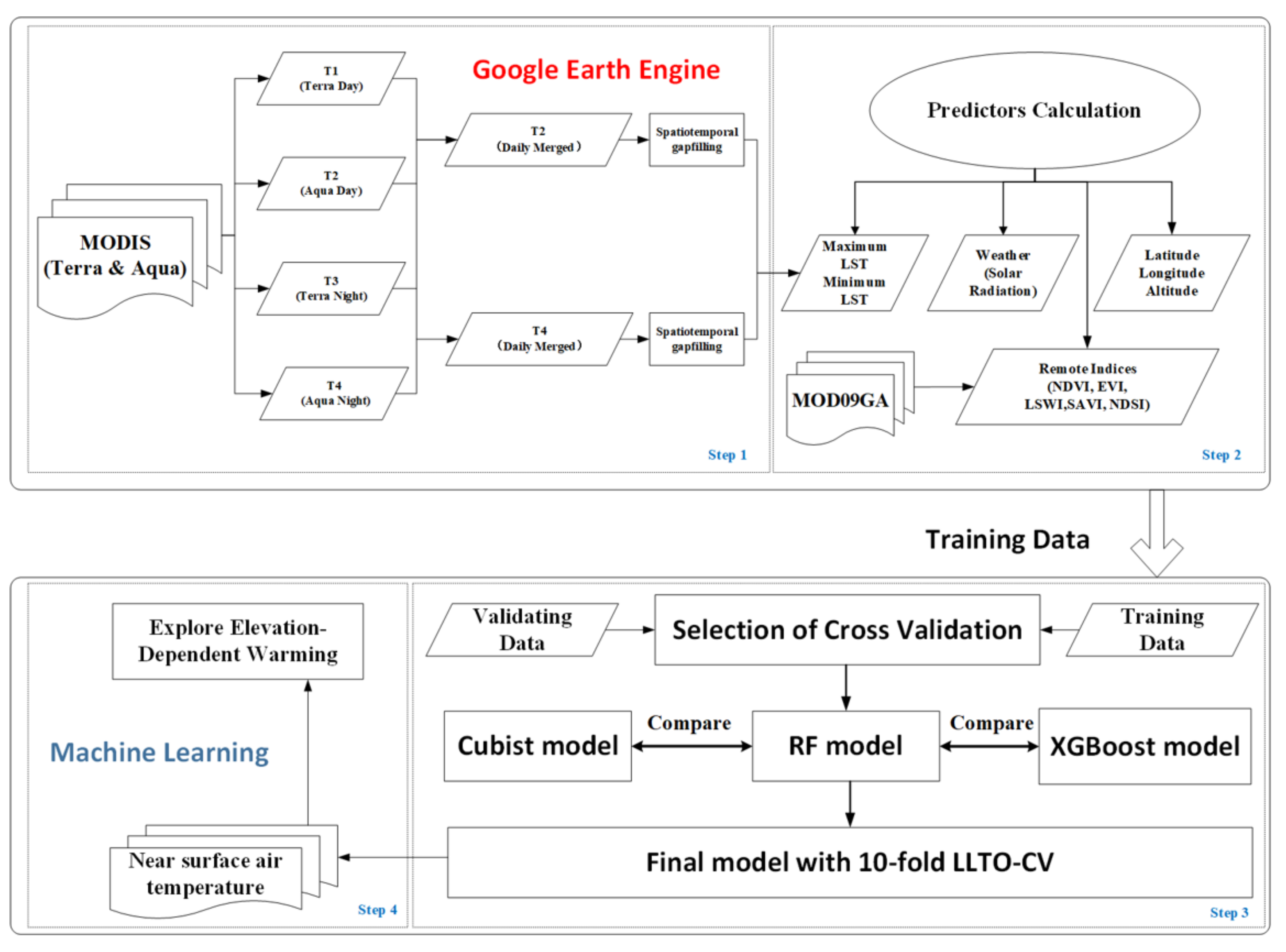
The TP is located at 26–40 N and 73–105 E degree. It has irregular topography with elevations varying between approximately 498 and 7198 m a.s.l. (above sea level) and generally increasing from northwest to southeast (Figure 1). As elevation increases, the landscape transitions from forests to alpine grassland and then bare rock, and finally to snow and ice [29]. The highest Himalayan mountains are on the southern edge of the TP, while the Kunlun Mountains are another high mountain chain on the northwest boundary. The headwater areas of major rivers in Asia lie in the south-eastern part of TP (Hengduan Mountains). Typical alpine permafrost lies in Bayan Har Mountains. The Qaidam Basin is the largest basin in the TP.

In this study, daily observations of Tmax, Tmin, Tmean, and sunshine duration (2000–2016) from 130 available China Meteorological Administration (CMA) stations were used; the altitude of these stations ranged from 1600 to 4800 m a.s.l. To keep consistency between MODIS LST pixels and ground observations, a relatively homogeneous LST validation site named A’rou was chosen, which was located on the northeast edge of the TP with an elevation of 3032 m a.s.l. The in situ LST was derived from the upwelling and downwelling longwave radiation fluxes from A’rou station using a radiation transfer equation. As different emissivity sources provide different accuracies in LST calculation, in this study, we used ASTER-derived emissivity, derived from clear-sky pixels of ASTER images from 2000 to 2008 covering the study area. The monthly mean Tair observation data over the TP in 1981–2010, used in this study as reference data, are from the China Meteorological Data Service Centre (http://data.cma.cn/site/index. html). Another dataset is from the China Meteorological Forcing Dataset (CMFD) for the period of 1979–2018, developed through the fusion of remote sensing products, reanalysing datasets and in situ station data with a spatial resolution of 0.1° and a temporal resolution of three hours. Due to its continuous temporal coverage and consistent quality, the CMFD is one of the most widely-used climate datasets for China [30]. In addition, TerraClimate is a global gridded dataset of meteorological and water balance variables at 2.5 arc-minute resolution (4000 m) from 1958 to 2020 [31]. TerraClimate updates with a monthly time step and is available at https://climate.northwestknowledge.net/ TERRACLIMATE. The input datasets used in this study are listed on

Table 1. Overview of datasets across the TP.

Data Source	Temporal Resolution	Spatial Resolution
DEM	2000	30 m
Weather Sites	2003–2013, daily
LST Site	2007–2011, 10-min
MOD11A1/MYD11A1	2002–Current, daily	1000 m
MOD09GA	2000–2020, daily	1000 m
CMFD	1979–2018, 3-hour	0.1 degree
TerraClimate	1958–2018, monthly	0.025 degree

.

2.2. Methodology

The spatio-temporal patterns of Tair in mountainous areas were quite complex due to the influence of landscape-scale physiographic factors. To address these problems, we developed a modelling framework for Tair (Figure 2). The first step was to apply a hybrid method (combine serval methods, i.e., daily merging and spatio-temporal gap-filling) to create seamless remotely sensed LST datasets. The second step was to calculate a set of predictors including LST datasets, mountainous solar radiation, biophysical factors and topography indices for surface air temperature modelling over the TP from 2003 to 2013. The calculations of the above two steps were all conducted in the Google Earth Engine (GEE) environment. Those predictors were then integrated as explanatory variables for machine learning models, while the in situ measurements were used as the response variables. To avoid the spatial-overfitting of machine learning models, target-oriented validation strategies were used. In the third step, the cross validation (CV) data was split into 10 folds using spatial ID and Year ID as splitting criteria to predict unknown points in time and unknown locations. Then, the best model for each month was used for final tuning with 10-fold Leave Location and Time Out-Cross Validation (LLTO-CV), allowing us to provide accurate monthly spatial maps of Tair over the TP. The final step was to evaluate the climate change in TP with monthly Tair datasets by comparison with other temperature products. More details are presented in the following subsections.

2.2.1. Step 1: Hybrid Model to Estimate Daily Seamless MODIS LST and Validation

The development of globally complete spatial-temporal daily LST images still faces many challenges. Considering the advantages of MODIS LST including 1000 m spatial resolution with high temporal resolution and the computing efficiency of different gap-filling methods, we used a three-step hybrid method to build daily LST. The first step was the daily merging method, which involved using values from the other three times on the same day to fill the missing values for a given time. For example, we estimated T2 from T1, T3 and T4 and obtained four time series of T2 (LSTday), and then composited them to get the merged LST on a daily basis. The details of this step were presented by Li and Zhou [17]. The benefit of the daily merging method of four observations is that it increases the spatial and temporal extent of the daily LST coverage. The second step was to use a spatio-temporal gap-filling method by estimating missing values with values of their neighbouring cells and days. Existing spatio-temporal gap-filling methods are all sensitive to parameter configurations. However, when applied at a global scale, a set of universal key parameters is difficult to select. In this study, we used a new spatio-temporal gap-filling algorithm instead of traditional gap-filling packages or software, as this method is computationally efficient and is promising for large scale applications. Especially, we chose 10,000 m as the searching radius of bicubic interpolation and 30 days as the given window for moving the average temporal interpolation. The third step was to use the Whittaker smoother to remove the outliers introduced by spatio-temporal filled LSTs. We noted that the hybrid method depended heavily on daily merging LSTs. Therefore, the daily merging LSTs were treated as good LSTs and the remaining gaps left after the daily merging were filled by Whittaker smoother values.

Validation of the land surface temperature used the radiation transfer equation below:

R_n = R_si − R_so + R_li − R_lo

(1)

where R_si, R_so, R_li, R_lo are incoming shortwave radiation (w·m⁻²), outgoing shortwave radiation (w·m⁻²), incoming longwave radiation (w·m⁻²), outgoing longwave radiation (w·m⁻²) respectively, R_n with the net radiation. In Equation (1), R_lo is a direct function of land surface temperature. For a surface with emissivity ε (unitless), the outgoing long-wave flux is composed of both reflected and emitted parts.

R_lo = (1 − ε) × R_li + ε × σ × T_s⁴

(2)

where σ is Stefan-Boltzmann constant (5.67 × 10⁻⁸ W m⁻² K⁻⁴) and T_s is land surface temperature. If R_li and R_lo were obtained from radiometric network, the accuracy of the land surface temperature would be dependent on emissivity ε.

2.2.2. Step 2: Remotely Sensed Indices, DEM Derivatives and Mountainous Solar Radiation

Due to the limited data availability from the TP, the model accuracy largely relies on the input datasets. If it is insufficiently trained, a robust correlation cannot be expected, that is, the more sufficient the samples, the better the spatial prediction accuracy [32]. MODIS Terra/Aqua LST products (MOD11A1 and MYD11A1) were obtained from NASA (https://lpdaac.usgs.gov/products/myd11a1v006/, https://lpdaac.usgs.gov/products/mod11a1v006/). The MODIS Terra overpass times are around local time 10:30 AM (T1) in descending mode and 10:30 PM (T2) in ascending mode. The MODIS Aqua overpass time is around 1:30 PM (T3) in ascending mode and 1:30 AM (T4) in descending mode. Time-variant biophysical factors, such as Normalized Difference Vegetation Index (NDVI), Enhanced Vegetation Index (EVI), Land Surface Water Index (LSWI), Normalized Difference Snow Index (NDSI), and Soil Adjusted Vegetation Index (SAVI), derived from MODIS surface reflectance bands, and which have the same spatial and temporal resolution as LST, were incorporated as training inputs for machine learning models. This study also produced incoming mountainous solar radiation dataset as a predictor of air temperature distribution in the TP, and provided a web app tool based on GEE for user access (https://geogismx.users.earthengine.app/view/tpmsr). In fact, the incoming mountainous solar radiation in TP was used the first time in this study, as previously such dataset did not exist or was not used as a variable in estimating air temperature over the TP. Therefore, with the availability of these topographical variables, weather datasets and biophysical indices for the TP, we were able to achieve a more reliable estimate on Tair in high mountainous area.

2.2.3. Step 3: Regression Models and Target-Oriented Validation

In this study, we adopted three commonly used regression techniques to reproduce Tair. From the literature review, it was suggested that the differences in land surface properties, solar radiation, topography and many other factors could influence the relationships between MODIS LST and Tair. Therefore, the linear regression model is unlikely to be able to handle the complicated relationship between Tair and the abovementioned variables under different conditions. In contrast, advanced machine learning models, such as Random Forest, Cubist and XGBoost, can take account of the nonlinear and complicated relationship between the predictor and response variables in a mountainous study area like the TP.

Random Forest (RF), also known as random decision forest, is an advanced ensemble machine learning technique which can be used to develop predictive models for both regression and classification purposes [33]. The ensemble technique is an algorithm that integrates outputs from multiple learning models to generate better predictions. In the case of RF, it achieves this goal by obtaining outputs from a whole forest of random decision trees. Decision trees are also a popular regression method, but they tend to overfit on training data and usually have high variance, even if utilizing different training and testing sets from a same dataset [34]. Nevertheless, decision trees can be used as an underlying foundation in ensemble methods to produce more accurate predictions. The RF first creates an ensemble of decision trees through a process of bagging (bootstrap aggregating). Randomised subsets of the predictors are assigned to each tree to generate predictions. The average of the predictions from the ensemble of the trees is treated as the final outcome [35]. Thus, the RF succeeds in reducing the variance by creating a majority-votes model. In recent years, RF has been frequently used in remote sensing-related research [36,37].

Extreme Gradient Boosting (XGBoost) is a scalable and efficient implementation of the gradient boosting framework [38]. It is also an ensemble technique that can build a final predictive model based on a larger number of underlying models. The most commonly used underlying model is a regression tree, different to RF. Another difference is that XGBoost repeatedly trains trees or the residuals of the previous predictors, while RF trains many independent trees and then averages them. In the present study, we adopted DART (Dropouts meet multiple Additive Regression Trees), an ensemble model of boosted regression trees, which is capable of overcoming the issue of “over-specialization” [39].

Cubist regression is a commercial, rule-based regression method that was developed based on a combination of the ideas of Quinlan [40]. For this reason, it lacks algorithmic documentation. After Cubist regression was introduced into R by Kuhn, it has been widely used in remote sensing studies. Unlike CART-based regression trees (e.g., RF) that have a final model, Cubist produces rule-based multivariate regression models, which means that a set of rules is associated with sets of multivariate regression. Then, an actual prediction model will be chosen based on the rule that best fits the predictors. Since Cubist generates rule-based results, it is more straightforward and interpretable than RF. Cubist has much shorter run times than CART-based regression trees.

K-fold Cross Validation is popular for estimations of the performance of the model with a view towards data that has not been used for model training. The validation dataset is randomly split into k folds during standard random k-fold Cross Validation. However, the problem of dependencies caused by the nature of spatial-temporal data was ignored, producing overly-optimistic model performance because of spatial-temporal overfitting [26,41,42]. To be more specific, many prediction models use auxiliary predictor variables which vary in space but not in time (e.g. elevation, location, and biophysical characters). However, temporally static variables that focus on describing the spatial characteristics of the climate stations are prone to enabling machine learning algorithms to disguise the real relationships between predictors and responses, and lead to spatial over-fitting. For example, the performance differences between K-fold random Cross Validation (lower RMSE) and Leave-Location-Out Cross Validation (higher RMSE) in the literature strongly suggest that spatio-temporal prediction models fail in the prediction beyond the location of training stations, but can very well predict the unknown time of the training stations.

As we aim to predict air temperature in unknown locations, we perform a target-oriented validation which validates the model with a view towards spatial mapping. To this end, we repeatedly leave the complete time series of one or more data loggers out, and use them as test data during CV. This study will use the following two steps to identify and avoid overfitting.

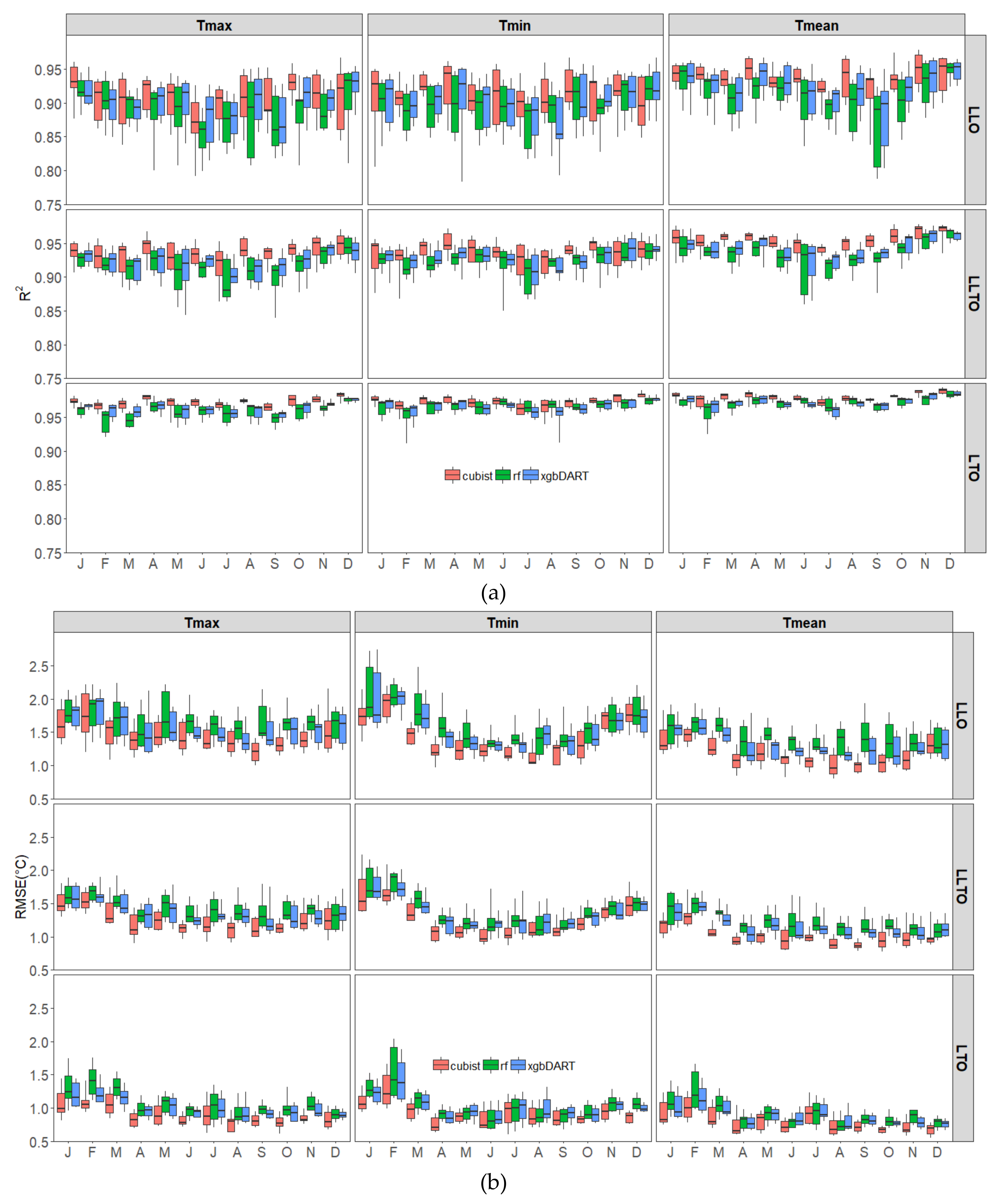
• To compare Machine Learning methods with different validation strategies using 10-fold Leave-Location-Time-Out (LLTO), Leave-Location-Out (LLO) and Leave-Time-Out (LTO).
• Using the best fitting model with suitable validation strategies to estimate monthly Tair products based on 10-fold LLTO Cross-Validation.

2.2.4. Step 4: Creating Near-Surface Air Temperature Products and Elevation-Dependent Warming Analysis

The controversy over the elevation-dependent nature of warming in the TP is mainly due to a lack of high-altitude meteorological data from the region [43]. In this paper, to obtain more reliable Tair products for elevation-dependent warming analyses, we produced 11 variables to build the actual nonlinear relationship with response, and tested three machine learning models with three different validation methods. According to the performance measurement of RMSE and R², RF was finally selected as the best model for Tair product generation. By comparing the accuracy of the three Tair products, the most accurate monthly mean air temperature during the period from 2003 to 2013 was selected to analyse the temperature change over TP.

Due to the wide spatial domain of the TP, temperature variations are inconsistent in different regions. Therefore, in this study, all the pixels in the three 1000 m elevation intervals were extracted and the time series of temperature changes in each elevation range were computed from the mean of the pixels. Specifically, we explore the relationship between temperature trends and elevations of 2000–3000 m, and 4000–5000 m and 6000–7000 m a.s.l., respectively. Among the analysis of temperature trends, the Seasonal Mann–Kendall statistical test and Seasonal Sen’s slope test [44] were employed to test the significances of trend and the magnitude of trend in the seasonal mean temperatures.

3. Results

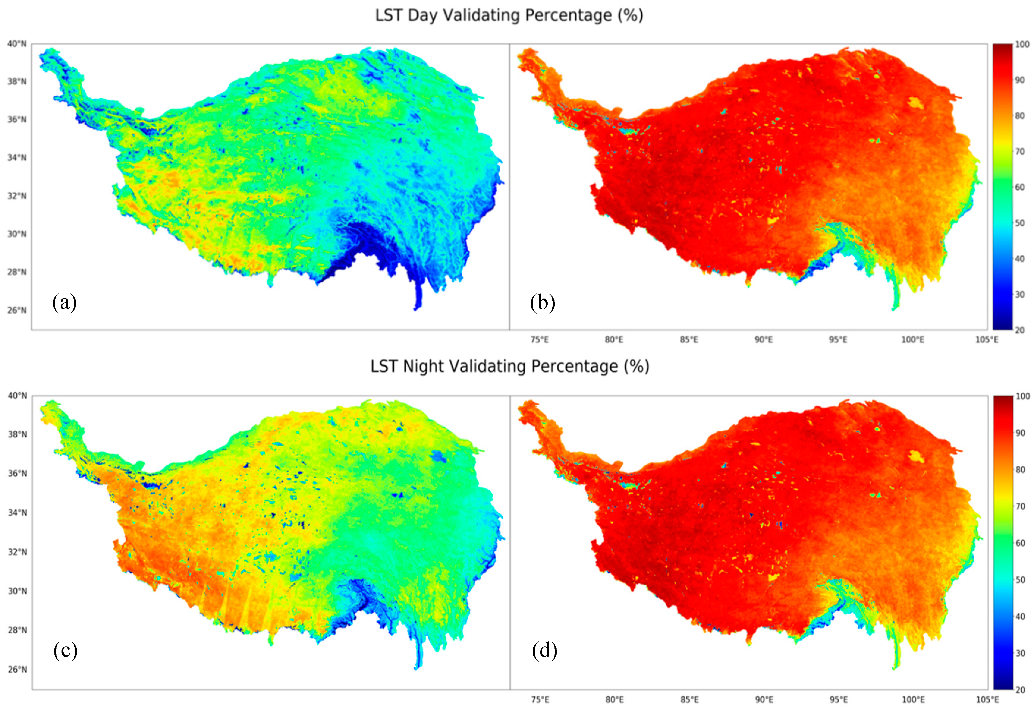
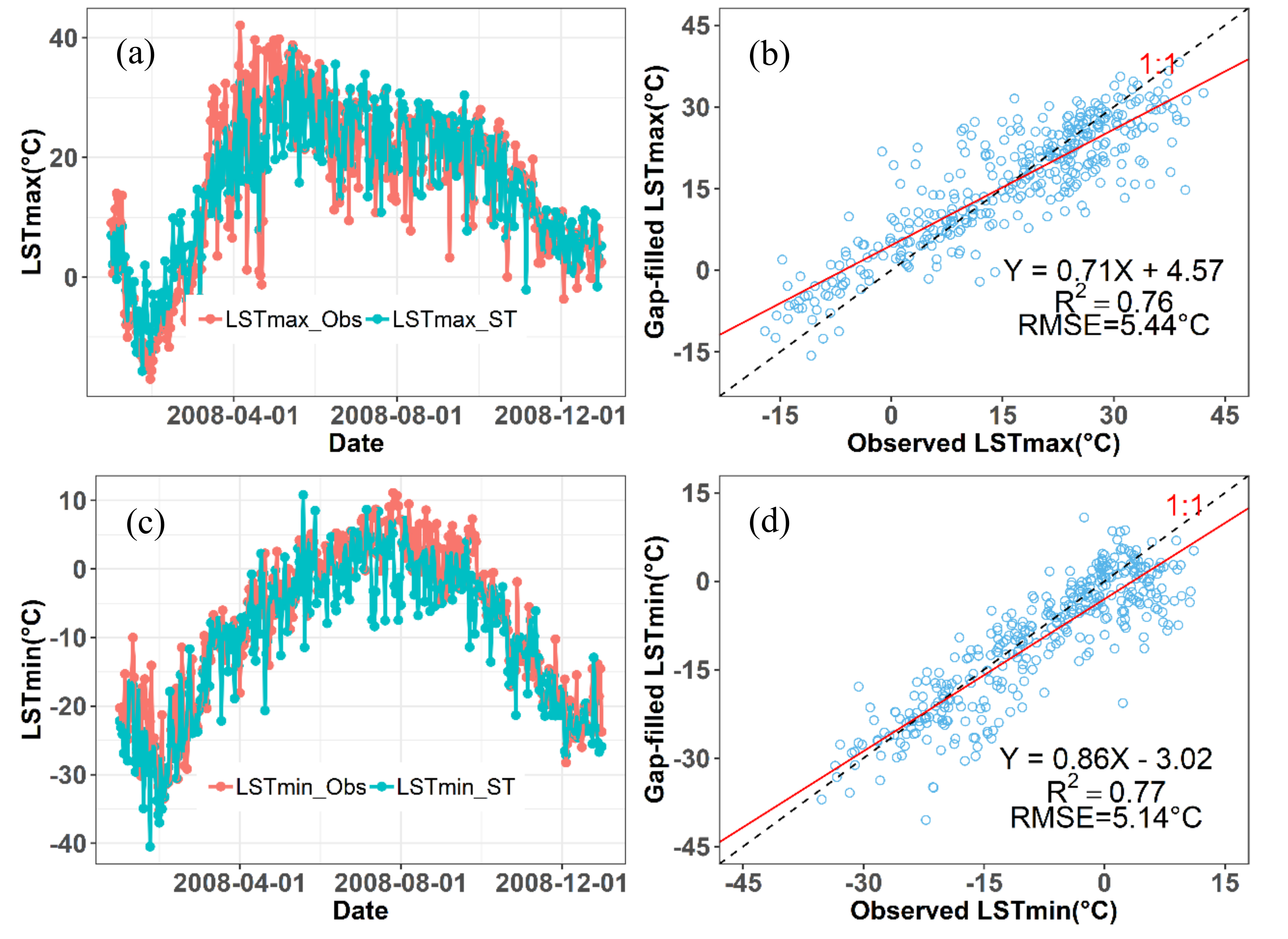
3.1. Evaluation of Spatio-Temporal Composite LST

Figure 3 shows the percentages of all available days per year for which maximum LST and minimum LST before and after using daily merging method. Overall, the percentage of MODIS LST data availability over TP is over 80%, while after daily merging, it is over 99%. For example, daily merging of the four observations increases most of LST data coverage by about 30% and 20% for LST day and LST night, respectively. In addition, a comparison of Figure 3a,c shows that the LST day value availability is intrinsically lower than that in LST night. For the central part of TP, the data coverage of the observed LST day is around 70%, while the data coverage LST night availability is about 80%. For the eastern part of TP, the available percentages for the observed LST day and night are about 45% and 60%, respectively. After merging daily LSTs from the four overpasses, LST coverage can increase to over 99% in central TP, and about 80% in eastern TP. However, it still fails to fill the gaps in the boundary of southern TP (see in Figure 3b,d). Therefore, an additional step is to use spatio-temporal gapfilling to fill the remaining missing values for the whole region.

To evaluate the accuracy of MODIS spatio-temporal composite LST, a ground measurement comparison at the A’rou station for 2008 was conducted for both maximum LST and minimum LST observations. The ground measurements at the nearest collection times matching with MODIS maximum and minimum LSTs were used. The annual comparisons are shown in the left panel of Figure 4. The scatterplots of the comparisons are given in the right panel of this figure. For the maximum LST comparison, the RMSE and R² over A’rou station were 5.44 °C and 0.76. For the minimum LST comparison, the RMSE and R² were 5.14 °C and 0.77. It should be noted that the minimum LST results were slightly better than for the maximum LST due to the stable weather conditions at night. From the annual results comparison, we can see that during the winter/spring when the freeze/thaw transition happens frequently, the differences of maximum LST or minimum LST with in situ measurements were greater than in other seasons.

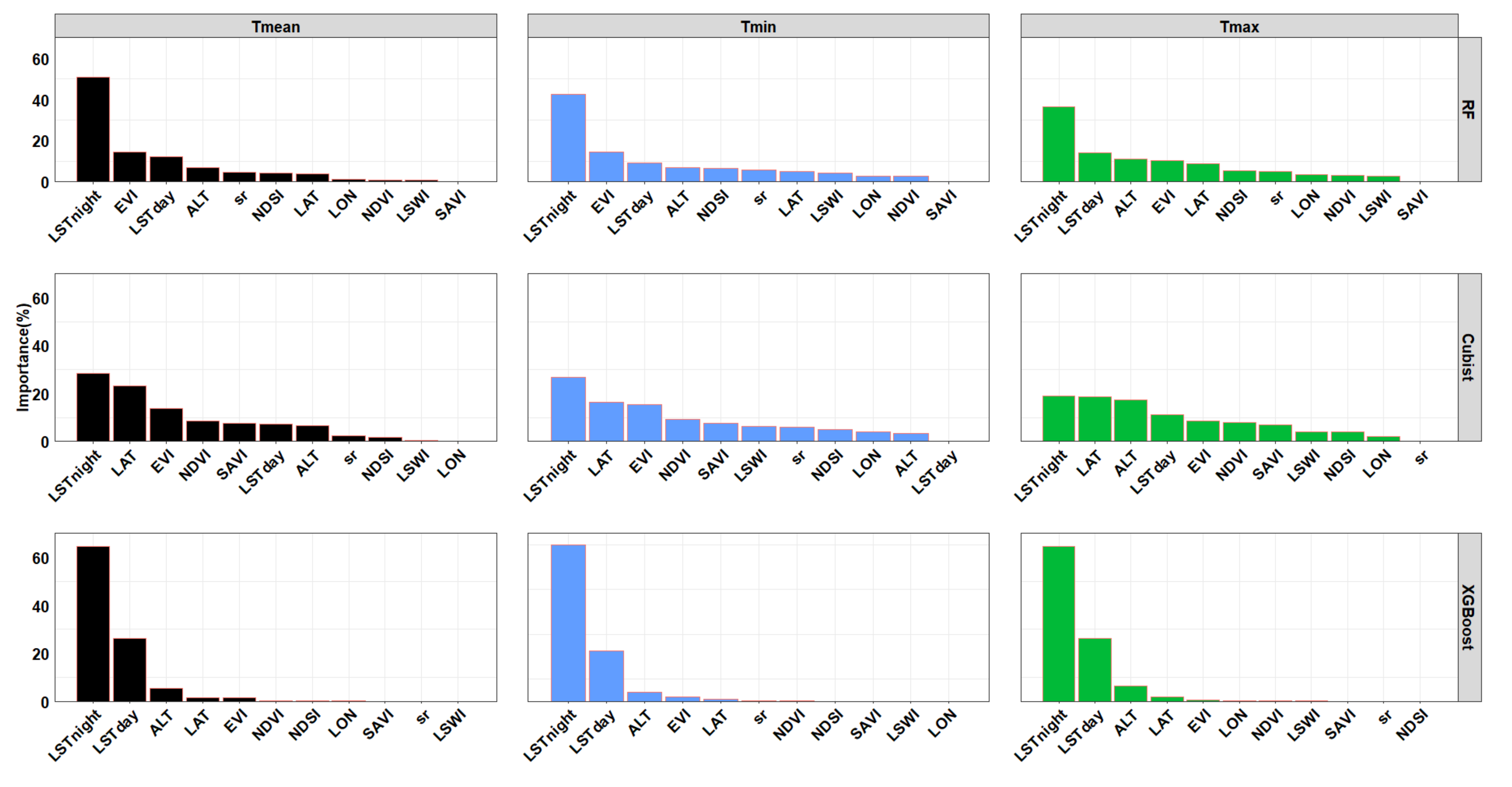
3.2. Model Performance and Variable Importance

Figure 5 shows that model performances differed from the different temperature products and the target-oriented validation methods. All the 27 models used in this study appeared to have strong relationships (R² > 0.75 and RMSE < 2.6 °C) at the monthly scale. For the three methods used, it can be clearly seen that Cubist regression always showed higher accuracy than XGBoost and RF, but RF was the most robust one with less outliers (not shown on Figure 5, R² < 1th percentiles and R² > 99th percentiles). In terms of the model performance for three temperature products, the Tmean had the highest accuracy and conversely, the Tmax had the lowest. From Tmax to Tmin to Tmean, the model performance increased, and the differences between RF, Cubist, XGBoost were getting smaller. Additionally, the model performance of LTO-CV was much better than that of LLO-CV and LLTO-CV. The changes of R² for different temperature products across 12 months was not obvious, but the RMSE showed apparent seasonal variation, i.e., higher in winter and lower in summer. Notably, the RMSE in August (the median RMSE is about 1.0 °C) were much lower compared to other months.

Variable importance for each Tmax, Tmin, and Tmean was determined by different Machine Learning methods based on LLTO-CV (Figure 6). For all properties in all plots, LSTnight explained most of the variable importance. LSTday was identified as being of major importance to the RF and XGBoost, but LSTday within the Cubist variable importance plots had limited influence on Tmax and Tmean, and its importance even dropped to zero in relation to Tmin. Meanwhile, the importance of elevation demonstrated by Cubist became progressively weaker from Tmax to Tmean, and Tmin. In contrast, RF and XGBoost identified elevation as a decisive factor in for temperature estimates. More specifically, elevation occupied the third or the fourth place in terms of importance in the plots of Random Forest, and always ranked in the top three within XGBoost plots. However, for the subplots using XGBoost, there was no clear influence for other variables except LSTday, LSTnight and elevation, where their total importance was higher than 95%. Unlike the XGBoost, other indices in the variable ranking plots demonstrated by Random Forest were also good predictors, while both LSTday and LSTnight showed great ability to improve the air temperature estimates. Therefore, these results revealed that RF had greater explanatory capability for temperature estimates than the other two machine learning methods. Modelled solar radiation, which was a predictor of Tair in complex terrain, also had good explanatory power, i.e., in the top five, within RF. The ranking results of other remotely sensed indices such as EVI and NDSI were as expected; vegetation had a close relationship with temperature, and snow cover change reflected by NDSI was an important indicatod of a warming/cooling climate.

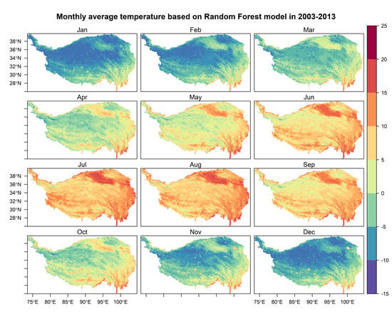
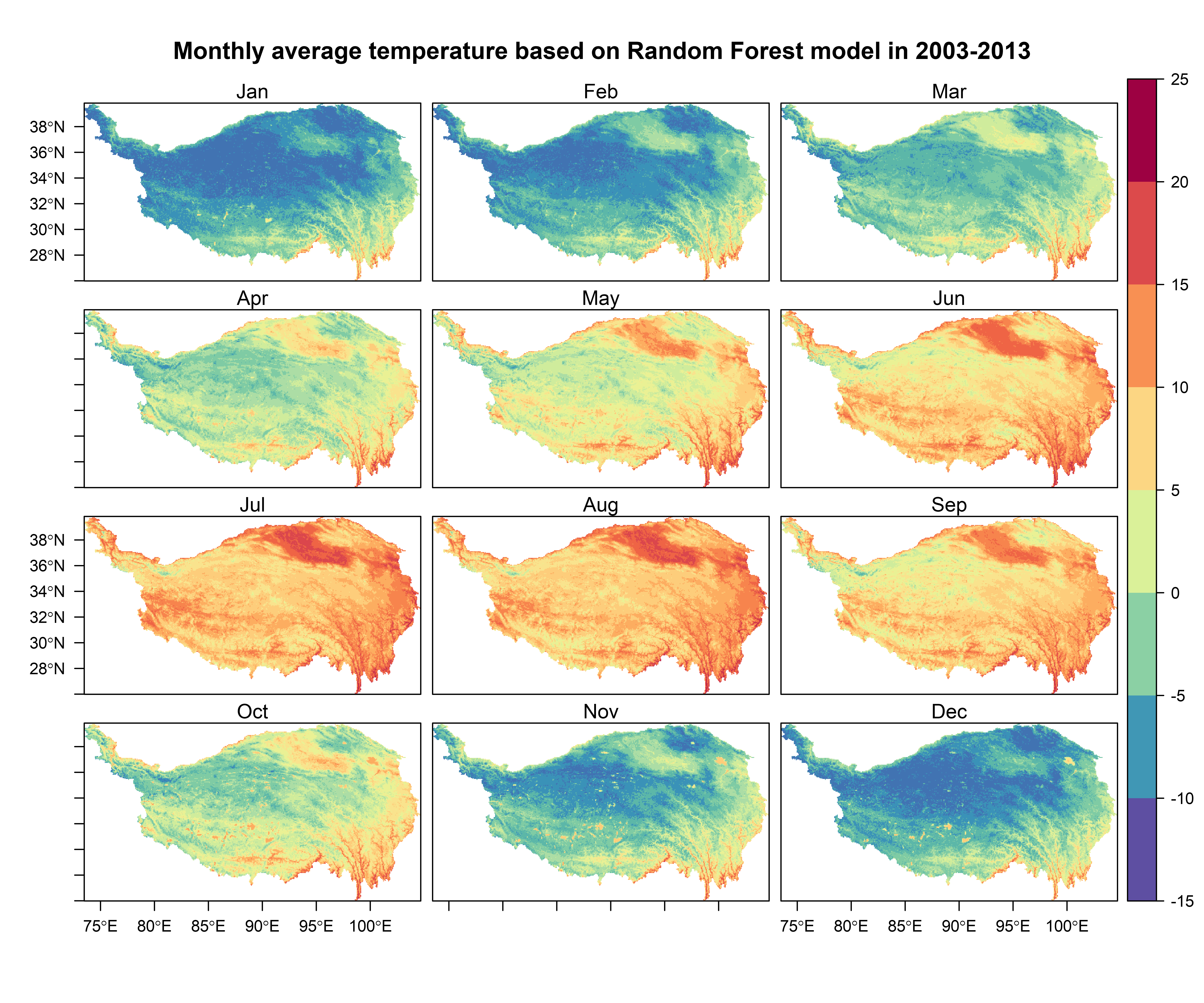
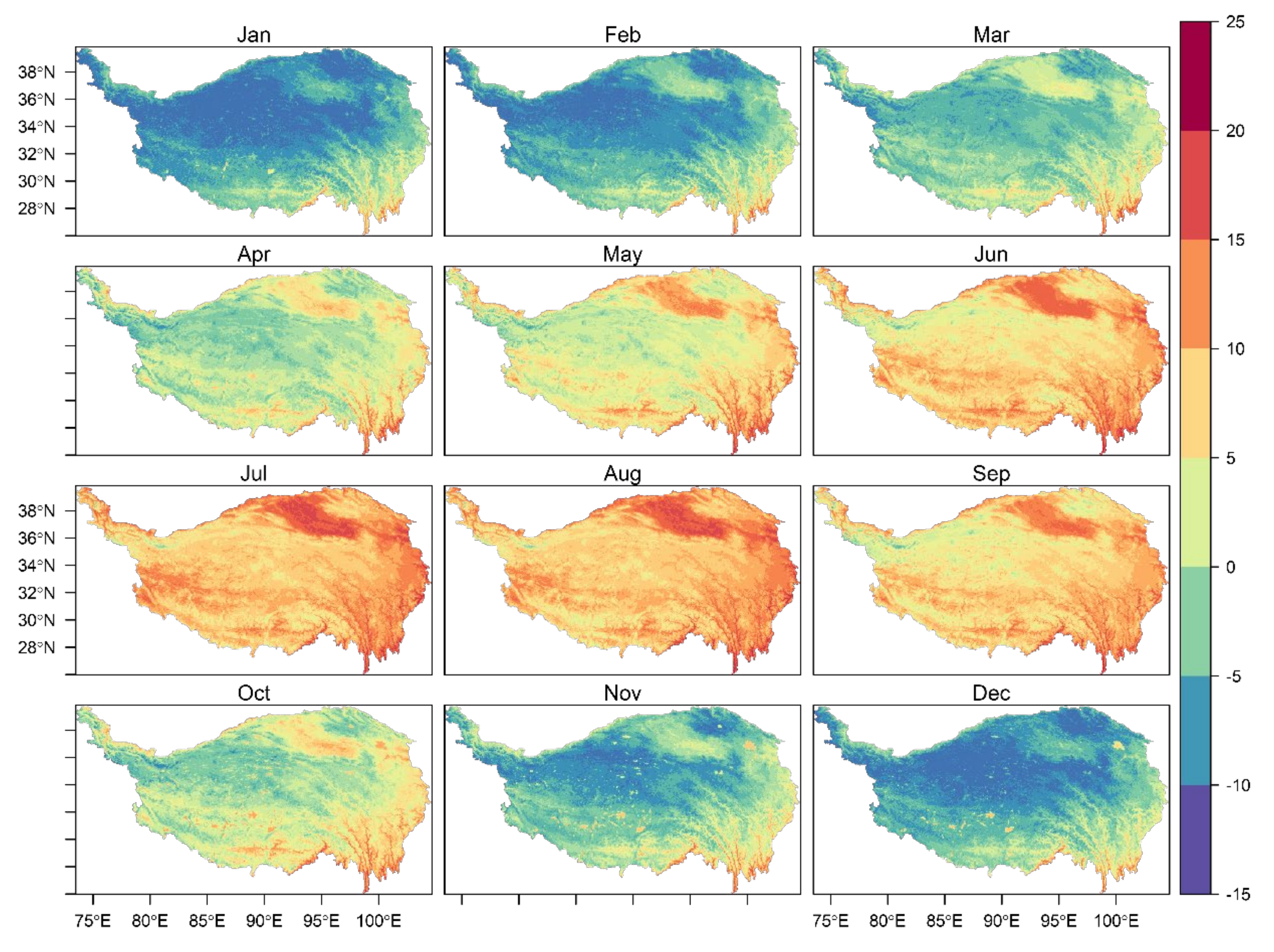
3.3. Spatial Distribution of Surface Air Temperature

As the monthly time step is more important for many long-term natural resource models, here, we focused on the spatio-temporal characteristics of monthly Tmean in 2003–2013 over the TP using both the station network and our modelling product. Spatially, the range of Tmean was from −15 °C to 20 °C across the TP (Figure 7). The warmest month was July and the coldest was January. Monthly Tmax and Tmin (see in Supplementary Materials Figure S2, Figure S3) generally followed similar spatial patterns; the northwest TP was the coldest area, gradually increasing toward the southeast, showing a stepped distribution. As areas in the south and east of the plateau are covered with lush vegetation and strongly influenced by the monsoon, they are amongst the hottest parts of the plateau. Meanwhile, the south eastern part of the plateau was the warmest, followed by the Qaidam Basin in the northeast, because of its relatively low altitude. In addition, we derived the seasonal mean and annual mean temperatures from the monthly mean temperature over the TP (see in Supplementary Materials Figure S1), with results similar to those of Zhang and Zhang [15].

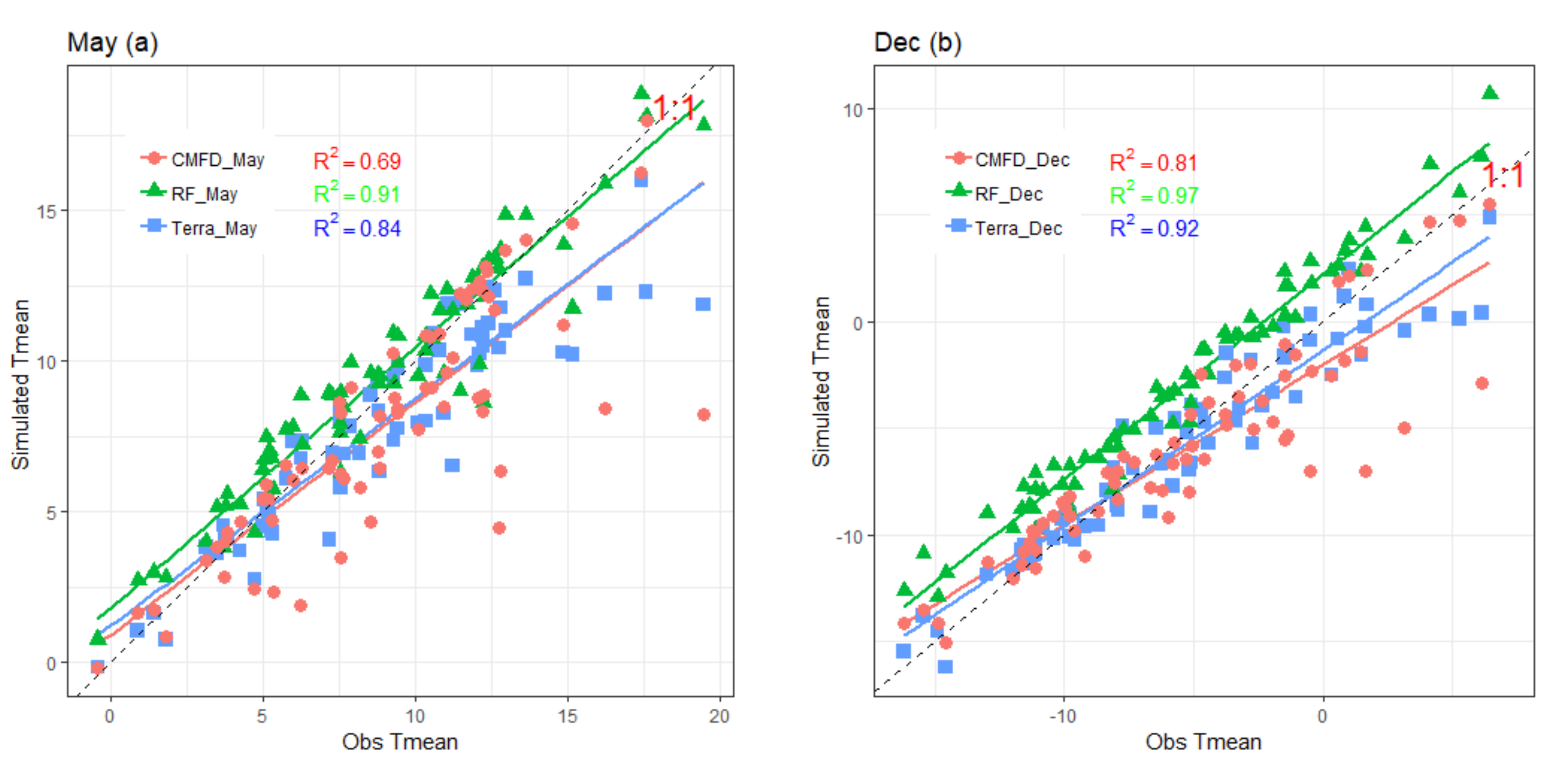
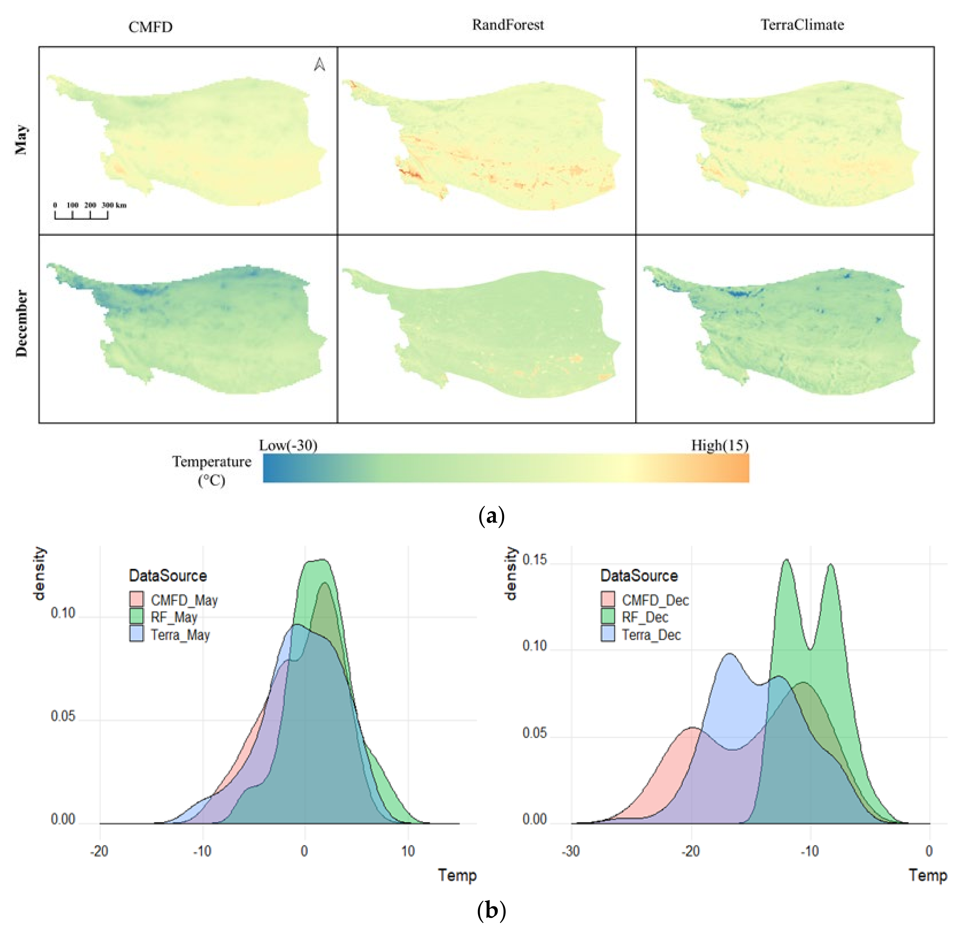
3.4. Comparison with Other Tibetan Plateau Temperature Products

The solar elevation angle in May is relatively high, and daytime ventilation and atmospheric mixing are generally great. In contrast, the lower solar elevation angle, longer night-time and more frequent radiative cooling in December result in colder air drainage and temperature inversions [45]. Thus, we used Tmean in May to compare the difference between our temperature product and others. Figure 8 shows the R² using different monthly air temperature products for May and December over the eastern plateau, with a dense concentration of climate stations. The Random Forest method resulted in R² values of 0.84 and 0.97 for May (Figure 8a) and December (Figure 8b) respectively. The monthly Tmean based on TerraClimate products had R² values of 0.79 for May and 0.91 for December. In contrast, CMFD showed a lower performance with R² of 0.55 for May and 0.78 for December. Thus, the accuracy of our product was better than other temperature products over the eastern TP.

The spatial maps of Tmean for May and December based on different products are shown in Figure 9a. The density plots from every pixel of those spatial maps are provided for comparison (Figure 9b). In May, a normal distribution of single peaks appeared; however, in December, a normal distribution of double peaks was observed. The mean values of the density curves in May were about the same, but the variance was different. In comparison, the difference was notable in the case of December, where mean temperatures from TerraClimate were much lower than those from our product. The density of mean temperature in December was in the range of −30 °C to −5 °C. However, according to Zhang, Zhang [15], the mean temperature in winter in the TP is mostly above −12 °C. This difference is partially due to the different models applied. In terms of Tmean generated from Random Forest, it tended to be warmer than the others. For the method applied in TerraClimate, the Tair in various regions of the world always has a positive relationship with elevation. According to the research of Cai and You [46], Tair in TP in the spring has a negative elevation dependency, while that in summer has a positive one. Based on the above conclusion, it is possible to understand the reason that Tair in May showed no obvious differences between the three products.

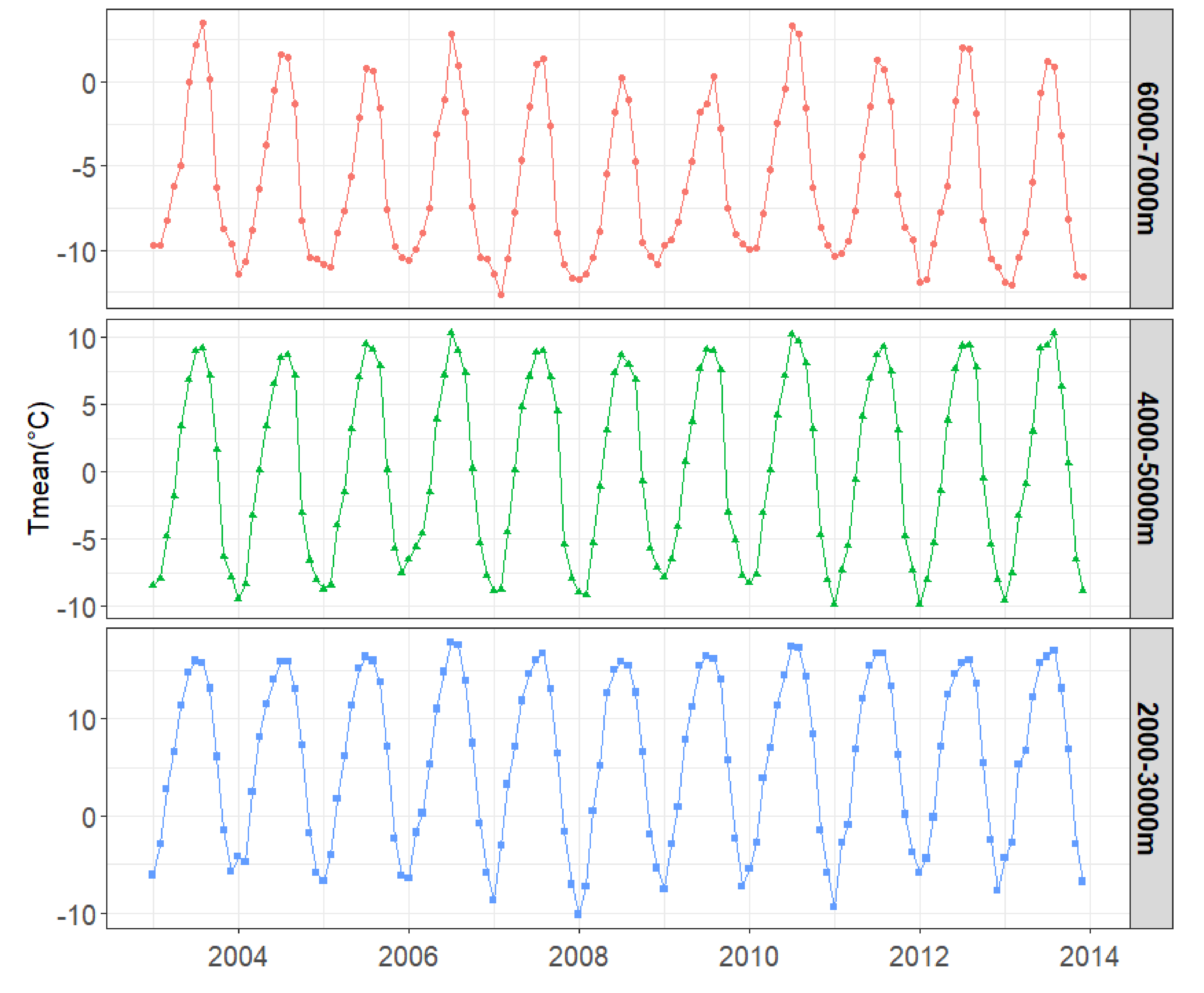
3.5. Elevation-Dependent Warming

Mean Tair products with the highest accuracy were used to explore the evidence of elevation-dependent warming over TP based on three representative elevation zones: 6000–7000 m, 4000–5000 m, and 2000–3000 m. As shown on Figure 10, in the period from 2003 to 2007, temperature increased in the elevation zones of 2000–3000 m and 4000–5000 m, while temperature decreased at 6000–7000 m. According to the seasonal Mann-Kendall test, only the temperature data in 6000–7000 m (p value = 0.003) showed a significant cooling trend, while the 2000–3000 m (0.37) and 4000–5000 m (0.11) data did not pass the test. In the period from 2003 to 2013, we found that a cooling trend was observed over 6000 m, but that the trends at 2000–3000 m and 4000–5000 m were not significant. Furthermore, when the seasonal Sen’s slope test was used, we found that the magnitude of the trend at 6000–7000 m (slope = −0.09) showed a negative tendency, while 2000–3000 m (slope = 0.02) and 4000–5000 m (0.04) both showed positive trends.

4. Discussion

In this study, we investigated the usefulness of a hybrid methodology to provide continuous remote-sensed LST for modelling Tair. The application of this methodology over the TP provides thorough datasets in data-sparse areas with high elevations by daily MODIS Terra/Aqua LST merging and spatio-temporal gap-filling. It is noteworthy that the missing pixels in the daily LST images after processing by the hybrid method still exist along the south-eastern boundary of the TP, where cloud-days are much more frequent than clear-sky days. Key map and figure results were illustrated in a web application (Hybrid MODIS LST Composite Online Tool, https://geogismx.users.earthengine.app/view/hybrid-modis-composite-lst). This web tool gives us instant access to the global-scale LST data archive and cloud computation capabilities of the GEE. Moreover, with this app link, the user can even acquire results from mobile devices, and does not need to install any software and third-party packages, as opposed to desktop applications. Other prospects for the application of this tool include obtaining high-resolution LSTs which would dynamically capture the urban heat island phenomenon at a fine scale. However, Leihy and Duffy [25] found great uncertainty in gap-fill predictions for missing LSTs at high elevation sites. For spatially- and temporally-neighboring predictions, further research needs to consider advanced spatio-temporal gap filling methods that account for the use of unique parameters for the pixel-specific gap patterns to fill in the missing values [47], especially in mountainous area.

The daily daytime and nighttime LST estimates from this study have good correlation (R² = 0.75) comparable to those of Ouyang and Chen [12],although they only used clear-sky AATSR products at the A’rou station for validation. However, due to the difficulty of obtaining representative LST data from ground LST measurements in TP, validation of LST at only one site (A’rou) cannot be deemed representative of the whole TP. Therefore, with the Hybrid MODIS LST online composite tools, more in situ LST measurements, if available, could be used for validations in the future. Additionally, the spatio-temporal model validation strategies in this study do not rely on random k-fold cross validation. Instead, stricter validation strategies such as LTO, LLO, and LLTO are used for comparisons. However, the aim of this study is to assess the error in both time and space; LLTO CV is finally used for the final target-oriented CV. According to Meyer and Reudenbach [26], Forward Feature Selection (FFS) in conjunction with LLTO makes it possible to remove variables that lead to overfitting. For example, the terrain related variables may contribute to overfitting, as these “static variables” are overrepresented in the predictor datasets. Considering the fact that the process of training a large number of datasets was time consuming for the FFS, and that it did not show strong evidence in improving model performance, FFS was not adopted in this study. However, care must be taken when choosing the variables for training. We avoided an overly-optimistic approach to temperature prediction by using the target-oriented validation (in this case LLTO); nonetheless, the temperature products still contained errors coming from the characteristics of machine learning algorithms which were not able to predict extreme values (i.e., very low and very high temperatures). Further work is needed to improve these spatio-temporal models to capture extreme or abnormal temperature in both spatial and temporal domains.

Although in situ observation data below 4000 m clearly show a significant warming trend in the TP, the rate of warming at high-elevation mountains is still unknown. As far as we know, the gridded Tair products in the world are commonly interpolated by spatio-temporal interpolation based on meteorological stations, even in areas like TP with sparse networks of weather stations. In other words, unknown Tair at other locations (such as high mountainous areas and valley areas) is estimated by what we know from locations. The key to the success and applicability of common spatio-temporal interpolation is the underlying assumption employed in describing the relationships and the way in which these relationships are characterised [32]. The underlying assumption of common spatio-temporal interpolation to estimate unknown Tair is that the values of target Tair are spatially autocorrelated. Locations which are closer would have more similar Tair values than locations which are further apart. Therefore, geographical variables such as elevation and distance are used to capture and represent spatio-temporal correlations through geostatistical methods (such as Kriging, IDW). However, geographical variables are consistently static, do not generally capture the temporal dynamics of the spatial pattern of the Tair, and cannot represent the effects of biophysical characteristics [48]. LST was used as a proxy for Tair, and has been successfully applied to estimate Tair for various regions of the world due to its ability to describe the surface-atmosphere energy exchange process. In this study, we used not just widely used auxiliary datasets (i.e., LST, locations, elevation, solar radiation and remotely sensed indices) to explicitly represent topographical and biophysical factors on Tair, but also adopted machine learning algorithms to handle the nonlinearity and highly correlated variables. Therefore, the proposed methods are technologically interoperable and scientifically rigorous for estimating Tair in mountainous areas. Improved satellite-based temperature Tair products may provide evidence of elevation-dependent warming. The validation results (Figure 8) indicate that the monthly gridded temperature maps show a potential to provide long-term Tair over TP compared to other independent coarse products. Such a product is of great necessity for data-scarce areas, and is therefore, critical for climate change research. As shown in Figure 10, before 2007, temperatures increased in the elevation zones of 2000–3000 m and 4000–5000 m, and decreased over 6000 m. This finding is consistent with findings in other research [49]. However, this result is debatable, because the period of analysis is extremely short. During the long period of 2003 to 2013, we found that the cooling trend over 6000 m was detected by seasonal Mann-Kendall test, and the warming patterns between 2000–3000 m and 4000–5000m were not obvious. This phenomenon was also observed by [29]. For instance, an increase in temperature was observed in parts of mountainous regions at around 4500–5500 m, whereas other mountainous regions observed limited temperature increases. However, according to previous landscape-scale research on Tair in mountainous environments [50], it is suggested that significant variations in temperature are occurring at elevation intervals of less than 1000 m. Minimum air temperature, with its strong sensitivity to cold-air drainage, is likely to vary at scales less than 200 m. It is believed that future improvements need to combine the distinct microclimates in high-mountain regions with high-resolution satellite-based datasets.

Unlike plain zones, which are relatively homogenous, mountain areas suffer from local variability, thus making it extremely difficult to ensure that the model simulation is perfect. Notwithstanding these limitations, the factors used for model simulation in this study have been shown to reflect temperature changes well. We found the predictor of NDSI to have a higher importance ranking than some other indices. As TP is one of the most sensitive areas to snow feedback on Earth, the shortened or prolonged snow cover duration in TP will influence the surface air temperature. You and Min [51] gave a further explanation that the rapid warming in TP is line with the decreasing snow cover, and hypothesised that changes in snow/ice cover expose the soil to wind or increase the snow line position and alter the absorption of solar radiation, leading to changes in surface temperature. Meanwhile, incoming solar radiation also plays a relatively important role in Tair estimations. Additionally, our results (Figure 5) show the model performance in estimating Tmin with night-time LST is better than Tmax using daytime LST. This difference can be partially explained by the fact that night-time LST is more stable than daytime LST. It is also of note that the model simulations are influenced by other climate factors and human activities, such as wind, relative humidity, cloud cover and land use change. However, these factors were not employed due to limited observations. Therefore, further studies considering more informative indices are needed to improve the simulations. For example, cloud cover over the TP shows a significant increasing trend; the supporting evidence for this is that there is a significant amount of atmospheric brown cloud generated by fossil fuel consumption and biomass burning over the Indian subcontinent and Asia which is transported to the TP by atmospheric circulation [52]. As we know, the presence of clouds interferes with the estimation of Tair in mountainous areas. That is probably part of the reason why the accuracy of the estimated Tair from the end of summer to the end of spring in the following year was not good (Figure 5). The most straightforward effect of cloud cover is that MODIS daily LST datasets suffer from a large number of missing values because of clouds and other atmospheric conditions (see in Figure 3a,c). Therefore, we adopted a hybrid approach (combining several methods) to fill the gaps in high spatio-temporal LST datasets before using them to estimate Tair. However, due to the lack of the cloud cover information, there is still a deviation between the gap-filled LST and the real LST on cloudy days. Another indirect effect of cloud cover is the estimation of other predictors (i.e., incoming solar radiation in TP). Instead of using a cloud-based model, a sunshine-based model was adopted to simulate incoming solar radiation under the influence of clouds. Therefore, if appropriate atmospheric parameters for the study area, such as cloud cover, atmospheric transmissivity and atmospheric turbidity can be obtained, the final modelling results would be better. In addition, factors like wind and relative humidity data also contribute to estimations of Tair. For example, weakening of the zonal wind speed was also shown to significantly raise the temperature in the Qaidam Basin [53].

5. Conclusions

In this study, we built an online tool based on a MODIS LST “hybrid” methodology to generate continuous daily maximum and minimum land surface temperature datasets in locations without observations, and to provide the required remotely sensed inputs to air temperature prediction models. Changes in received solar energy among mountains inevitably affect the earth’s energy budget. We integrate mountain solar radiation and diverse remotely sensed vegetation indices to provide reliable temperature products for the TP. By comparing the performance of different machine learning techniques, we found that the RF model performed best in predicting Tmax, Tmin, and Tmean. The methodology that we have developed could be useful for improving temperature datasets in mountainous regions around the globe, thereby also improving climatic, environmental, hydrological and ecological models.

References

1. Qiu, J. The third pole. Nature 2008, 454, 393–396. [Google Scholar] [CrossRef] [PubMed] [Green Version]
2. Manabe, S.; Terpstra, T. The effects of mountains on the general circulation of the atmosphere as identified by numerical experiments. J. Atmos. Sci. 1974, 31, 3–42. [Google Scholar] [CrossRef]
3. Duan, A.; Wu, G.; Liu, Y.; Ma, Y.; Zhao, P. Weather and climate effects of the Tibetan Plateau. Adv. Atmos. Sci. 2012, 29, 978–992. [Google Scholar] [CrossRef]
4. Kuang, X.; Jiao, J.J. Review on climate change on the Tibetan plateau during the last half century. J. Geophys. Res. Atmos. 2016, 121, 3979–4007. [Google Scholar] [CrossRef]
5. Kang, S.; Xu, Y.; You, Q.; Flügel, W.A.; Pepin, N.; Yao, T. Review of climate and cryospheric change in the Tibetan Plateau. Environ. Res. Lett. 2010, 5, 015101. [Google Scholar] [CrossRef]
6. Yang, K.; Wu, H.; Qin, J.; Lin, C.; Tang, W.; Chen, Y. Recent climate changes over the Tibetan Plateau and their impacts on energy and water cycle: A review. Glob. Planet. Chang. 2014, 112, 79–91. [Google Scholar] [CrossRef]
7. Dimri, A.P.; Bookhagen, B.; Stoffel, M.; Yasunari, T. Himalayan Weather and Climate and their Impact on the Environment. In Himalayan Weather and Climate and their Impact on the Environment; Springer Nature: Stuttgart, Germany, 2019. [Google Scholar]
8. Pepin, N.; Bradley, R.S.; Diaz, H.F.; Baraer, M.; Caceres, E.B.; Forsythe, N.; Fowler, H.; Greenwood, G.; Hashmi, M.Z.; Liu, X.D.; et al. Elevation-dependent warming in mountain regions of the world. Nat. Clim. Chang. 2015, 5, 424–430. [Google Scholar]
9. Fu, P.; Xie, Y.; Weng, Q.; Myint, S.; Meacham-Hensold, K.; Bernacchi, C. A physical model-based method for retrieving urban land surface temperatures under cloudy conditions. Remote Sens. Environ. 2019, 230, 111191. [Google Scholar] [CrossRef]
10. Anderson, M.C.; Norman, J.M.; Kustas, W.P.; Houborg, R.; Starks, P.J.; Agam, N. A thermal-based remote sensing technique for routine mapping of land-surface carbon, water and energy fluxes from field to regional scales. Remote Sens. Environ. 2008, 112, 4227–4241. [Google Scholar] [CrossRef]
11. Mallick, K.; Jarvis, A.J.; Boegh, E.; Fisher, J.B.; Drewry, D.T.; Tu, K.P.; Hook, S.J.; Hulley, G.; Ardö, J.; Beringer, J.; et al. A Surface Temperature Initiated Closure (STIC) for surface energy balance fluxes. Remote Sens. Environ. 2014, 141, 243–261. [Google Scholar] [CrossRef]
12. Ouyang, X.; Chen, D.; Duan, S.-B.; Lei, Y.; Dou, Y.; Hu, G.J.R.S. Validation and analysis of long-term AATSR land surface temperature product in the Heihe River basin, China. Remote Sens. 2017, 9, 152. [Google Scholar] [CrossRef] [Green Version]
13. Noi, P.; Degener, J.; Kappas, M. Comparison of multiple linear regression, cubist regression, and random forest algorithms to estimate daily air surface temperature from dynamic combinations of modis lst data. Remote Sens. 2017, 9, 398. [Google Scholar] [CrossRef] [Green Version]
14. Yang, Y.; Cai, W.; Yang, J. Evaluation of MODIS land surface temperature data to estimate near-surface air temperature in northeast China. Remote Sens. 2017, 9, 410. [Google Scholar] [CrossRef] [Green Version]
15. Zhang, H.; Zhang, F.; Ye, M.; Che, T.; Zhang, G. Estimating daily air temperatures over the Tibetan Plateau by dynamically integrating MODIS LST data. J. Geophys. Res. Atmos. 2016, 121, 11–425,441. [Google Scholar] [CrossRef] [Green Version]
16. Crosson, W.L.; Al-Hamdan, M.Z.; Hemmings, S.N.J.; Wade, G.M. A daily merged MODIS Aqua–Terra land surface temperature data set for the conterminous United States. Remote Sens. Environ. 2012, 119, 315–324. [Google Scholar] [CrossRef]
17. Li, X.; Zhou, Y.; Asrar, G.R.; Zhu, Z. Creating a seamless 1 km resolution daily land surface temperature dataset for urban and surrounding areas in the conterminous United States. Remote Sens. Environ. 2018, 206, 84–97. [Google Scholar] [CrossRef]
18. Zhu, W.; Lű, A.; Jia, S. Estimation of daily maximum and minimum air temperature using MODIS land surface temperature products. Remote Sens. Environ. 2013, 130, 62–73. [Google Scholar] [CrossRef]
19. Stisen, S.; Sandholt, I.; Nørgaard, A.; Fensholt, R.; Eklundh, L.J.R.S.O.E. Estimation of diurnal air temperature using MSG SEVIRI data in West Africa. Remote Sens. Environ. 2007, 110, 262–274. [Google Scholar] [CrossRef]
20. Kilibarda, M.; Hengl, T.; Heuvelink, G.B.M.; Gräler, B.; Pebesma, E.; Perčec Tadić, M.; Bajat, B. Spatio-temporal interpolation of daily temperatures for global land areas at 1 km resolution. J. Geophys. Res. Atmos. 2014, 119, 2294–2313. [Google Scholar] [CrossRef] [Green Version]
21. Metz, M.; Andreo, V.; Neteler, M. A New Fully Gap-Free Time Series of Land Surface Temperature from MODIS LST Data. Remote Sens. 2017, 9, 1333. [Google Scholar] [CrossRef] [Green Version]
22. Zhu, X.; Zhang, Q.; Xu, C.; Sun, P.; Hu, P. Reconstruction of high spatial resolution surface air temperature data across China: A new geo-intelligent multisource data-based machine learning technique. Sci. Total Environ. 2019, 665, 300–313. [Google Scholar] [CrossRef] [PubMed]
23. Yoo, C.; Im, J.; Park, S.; Quackenbush, L.J. Estimation of daily maximum and minimum air temperatures in urban landscapes using MODIS time series satellite data. ISPRS J. Photogramm. Remote Sens. 2018, 137, 149–162. [Google Scholar] [CrossRef]
24. Kalra, A.; Ahmad, S. Using oceanic-atmospheric oscillations for long lead time streamflow forecasting. Water Resour. Res. 2009, 45. [Google Scholar] [CrossRef]
25. Leihy, R.I.; Duffy, G.A.; Nortje, E.; Chown, S.L. High resolution temperature data for ecological research and management on the Southern Ocean Islands. Sci. Data 2018, 5, 180177. [Google Scholar] [CrossRef]
26. Meyer, H.; Reudenbach, C.; Hengl, T.; Katurji, M.; Nauss, T. Improving performance of spatio-temporal machine learning models using forward feature selection and target-oriented validation. Environ. Model. Softw. 2018, 101, 1–9. [Google Scholar] [CrossRef]
27. Bristow, K.L.; Campbell, G.S. On the relationship between incoming solar radiation and daily maximum and minimum temperature. Agric. For. Meteorol. 1984, 31, 159–166. [Google Scholar] [CrossRef]
28. Zhang, M.; Wang, B.; Liu, D.L.; Liu, J.; Zhang, H.; Feng, P.; Kong, D.; Cleverly, J.; Yang, X.; Yu, Q. Incorporating dynamic factors for improving a GIS-based solar radiation model. Trans. GIS 2020. [Google Scholar] [CrossRef]
29. Pepin, N.; Deng, H.; Zhang, H.; Zhang, F.; Kang, S.; Yao, T. An Examination of Temperature Trends at High Elevations Across the Tibetan Plateau: The Use of MODIS LST to Understand Patterns of Elevation-Dependent Warming. J. Geophys. Res. Atmos. 2019, 124, 5738–5756. [Google Scholar] [CrossRef] [Green Version]
30. He, J.; Yang, K.; Tang, W.; Lu, H.; Qin, J.; Chen, Y.; Li, X. The first high-resolution meteorological forcing dataset for land process studies over China. Sci. Data 2020, 7. [Google Scholar] [CrossRef] [Green Version]
31. Abatzoglou, J.T.; Dobrowski, S.Z.; Parks, S.A.; Hegewisch, K.C. TerraClimate, a high-resolution global dataset of monthly climate and climatic water balance from 1958-2015. Sci. Data 2018, 5, 171091. [Google Scholar] [CrossRef] [Green Version]
32. Zhu, A.X.; Lu, G.; Liu, J.; Qin, C.Z.; Zhou, C. Spatial prediction based on Third Law of Geography. Ann. GIS 2018, 24, 225–240. [Google Scholar] [CrossRef]
33. Breiman, L. Random forest. Mach. Learn. 2001, 45, 5–32. [Google Scholar] [CrossRef] [Green Version]
34. Olaru, C.; Wehenkel, L. A complete fuzzy decision tree technique. Fuzzy Sets Syst. 2003, 138, 221–254. [Google Scholar] [CrossRef] [Green Version]
35. Cutler, D.R.; Edwards, T.C.; Beard, K.H.; Cutler, A.; Hess, K.T. Random forests for classification in ecology. Ecology 2007, 88, 2783–2792. [Google Scholar] [CrossRef] [PubMed]
36. Moreno-Martínez, Á.; Camps-Valls, G.; Kattge, J.; Robinson, N.; Reichstein, M.; van Bodegom, P.; Kramer, K.; Cornelissen, J.H.C.; Reich, P.; Bahn, M.J.R.S.O.E. A methodology to derive global maps of leaf traits using remote sensing and climate data. Remote Sens. Environ. 2018, 218, 69–88. [Google Scholar] [CrossRef] [Green Version]
37. Hashimoto, H.; Wang, W.; Melton, F.S.; Moreno, A.L.; Ganguly, S.; Michaelis, A.R.; Nemani, R.R. High-resolution mapping of daily climate variables by aggregating multiple spatial data sets with the random forest algorithm over the conterminous United States. Int. J. Climatol. 2019, 39, 2964–2983. [Google Scholar] [CrossRef]
38. Friedman, J.H. Greedy function approximation: A gradient boosting machine. Ann. Stat. 2001, 29, 1189–1232. [Google Scholar] [CrossRef]
39. Rashmi, K.V.; Gilad-Bachrach, R. DART: Dropouts meet Multiple Additive Regression Trees. In Proceedings of the AISTATS, San Diego, CA, USA, 9–12 May 2015. [Google Scholar]
40. Quinlan, J.R. Learning with continuous classes. In Proceedings of the 5th Australian Joint Conference on Artificial Intelligence, Hobart, Astralia, 16–18 November 1992; pp. 343–348. [Google Scholar]
41. Gasch, C.K.; Hengl, T.; Gräler, B.; Meyer, H.; Magney, T.S.; Brown, D.J.J.S.S. Spatio-temporal interpolation of soil water, temperature, and electrical conductivity in 3D+ T: The Cook Agronomy Farm data set. Spat. Stat. 2015, 14, 70–90. [Google Scholar] [CrossRef]
42. Meyer, H.; Katurji, M.; Appelhans, T.; Müller, M.; Nauss, T.; Roudier, P.; Zawar-Reza, P.J.R.S. Mapping daily air temperature for Antarctica based on MODIS LST. Remote Sens. 2016, 8, 732. [Google Scholar] [CrossRef] [Green Version]
43. Li, B.; Chen, Y.; Shi, X. Does elevation dependent warming exist in high mountain Asia? Environ. Res. Lett. 2020, 15. [Google Scholar] [CrossRef]
44. Hirsch, R.M.; Slack, H.R.; Smith, R.A. Techniques of trend analysis for monthly water quality data. Water Resour. Res. 1982, 18, 107–121. [Google Scholar] [CrossRef] [Green Version]
45. Daly, C.; Conklin, D.R.; Unsworth, M.H. Local atmospheric decoupling in complex topography alters climate change impacts. Int. J. Climatol. 2009, 30, 1857–1864. [Google Scholar] [CrossRef]
46. Cai, D.; You, Q.; Fraedrich, K.; Guan, Y. Spatiotemporal Temperature Variability over the Tibetan Plateau: Altitudinal Dependence Associated with the Global Warming Hiatus. J. Clim. 2017, 30, 969–984. [Google Scholar] [CrossRef]
47. Kong, D.; Zhang, Y.; Gu, X.; Wang, D.J.I.J.O.P.; Sensing, R. A robust method for reconstructing global MODIS EVI time series on the Google Earth Engine. ISPRS J. Photogramm. Remote Sens. 2019, 155, 13–24. [Google Scholar] [CrossRef]
48. Li, X.; Zhou, Y.; Asrar, G.R.; Zhu, Z. Developing a 1 km resolution daily air temperature dataset for urban and surrounding areas in the conterminous United States. Remote Sens. Environ. 2018, 215, 74–84. [Google Scholar] [CrossRef]
49. Qin, J.; Yang, K.; Liang, S.; Guo, X. The altitudinal dependence of recent rapid warming over the Tibetan Plateau. Clim. Chang. 2009, 97, 321. [Google Scholar] [CrossRef]
50. Todd, R.L.; Dean, L.U. Spatial estimation of air temperature differences for landscape-scale studies in montane environments. Agric. For. Meteorol. 2003, 114, 141–151. [Google Scholar]
51. You, Q.; Min, J.; Kang, S. Rapid warming in the Tibetan Plateau from observations and CMIP5 models in recent decades. Int. J. Climatol. 2016, 36, 2660–2670. [Google Scholar] [CrossRef]
52. Ramanathan, V.; Ramana, M.V.; Roberts, G.; Kim, D.; Corrigan, C.; Chung, C.; Winker, D. Warming trends in Asia amplified by brown cloud solar absorption. Nature 2007, 448, 575–578. [Google Scholar] [CrossRef]
53. Wang, X.; Yang, M.; Liang, X.; Pang, G.; Wan, G.; Chen, X.; Luo, X. The dramatic climate warming in the Qaidam Basin, northeastern Tibetan Plateau, during 1961–2010. Int. J. Climatol. 2014, 34, 1524–1537. [Google Scholar] [CrossRef]
Figure 1. Location of TP, distribution of 130 weather stations and A’rou station.
Remotesensing 12 01722 g001
Figure 2. Flowchart of steps for calculation of near-surface temperature over TP.
Remotesensing 12 01722 g002
Figure 3. The percentages of available data in the two pairs of maps. (a) shows the percentage of days for the given year for which LST day (i.e., 1:30 pm on Aqua (T2)) values are available at each pixel of the TP domain. (b) shows the percentage of daily merged T2 for the given year for which daily merged T2 values are available. (c) shows the percentage of days for the given year for which LST night (i.e., 1:30 am on Aqua (T4)) values are available at each pixel of the TP domain. (d) shows the percentage of daily merged T4 for the given year for which daily merged T4 values are available.
Remotesensing 12 01722 g003
Figure 4. LST maximum and minimum temperature validation with in situ LST measurements in A’rou station. (a) and (b) show annual daytime comparison at A’rou site. (c) and (d) show annual nighttime comparison at A’rou site.
Remotesensing 12 01722 g004
Figure 5. (a) and (b) show the R2 and RMSE for maximum (Tmax), minimum (Tmin) and mean (Tmean) air temperatures using rf, cubist and xgbDART methods based on LLTO-CV, LTO-CV, LLO-CV. The boundaries of box mark the 25th and 75th percentiles; the horizontal black lines within the box indicate the median; the upper and lower whiskers mark the 90th and 10th percentiles.
Remotesensing 12 01722 g005
Figure 6. Tmean, Tmin, and Tmax temperature residuals showed varying temporal sensitivity to physiographic drivers. Each variable was scaled to a total of 100%.
Remotesensing 12 01722 g006
Figure 7. Monthly Tmean based on RF model in 2003–2013.
Remotesensing 12 01722 g007
Figure 8. Comparison of monthly Tmean in May (a) and December (b) derived from Random Forest, TerraClimate and CMFD with the observed mean temperature of 1980–2010 from in situ measurements.
Remotesensing 12 01722 g008
Figure 9. (a) Spatial average maps and (b) histograms of Tmean in 2003–2013 at Central TP for May and December.
Remotesensing 12 01722 g009
Figure 10. Tmean variation at three elevation zones from January 2003 to December 2013. The number of pixels within 1000 m elevation interval was extracted and each temperature change was computed from the mean of the pixels.
Remotesensing 12 01722 g010