Article

Monitoring Water-Related Ecosystems with Earth Observation Data in Support of Sustainable Development Goal (SDG) 6 Reporting

1
NASA Goddard Space Flight Center, 8800 Greenbelt Rd, Greenbelt, MD 20771, USA
2
USDA Forest Service Washington Office, 201 14th Street SW, Washington, DC 20024, USA
3
Science Systems and Applications, Inc., 10210 Greenbelt Road, Suite 600 Lanham, MD 20706, USA
4
Department of Geographical Sciences, University of Maryland, College Park, MD 20742, USA
5
Department of Coastal Studies, East Carolina University, Wanchese, NC 27948, USA
6
School of Computer, Mathematics & Natural Sciences, Morgan State University, 1700 E Cold Spring Ln, Montebello D302, Baltimore, MD 21251, USA
7
Booz Allen Hamilton, NASA Headquarters, 300 E St SW, Mail Suite: 3S67, Washington, DC 20546, USA
8
NOAA National Weather Service, 1325 East West Highway, Silver Spring, MD 20910, USA
9
Massachusetts Institute of Technology, 77 Massachusetts Avenue, Cambridge, MA 02139, USA
*
Author to whom correspondence should be addressed.
Remote Sens. 2020, 12(10), 1634; https://doi.org/10.3390/rs12101634
Submission received: 2 March 2020 / Revised: 11 May 2020 / Accepted: 12 May 2020 / Published: 20 May 2020

Abstract

:
Lack of national data on water-related ecosystems is a major challenge to achieving the Sustainable Development Goal (SDG) 6 targets by 2030. Monitoring surface water extent, wetlands, and water quality from space can be an important asset for many countries in support of SDG 6 reporting. We demonstrate the potential for Earth observation (EO) data to support country reporting for SDG Indicator 6.6.1, ‘Change in the extent of water-related ecosystems over time’ and identify important considerations for countries using these data for SDG reporting. The spatial extent of water-related ecosystems, and the partial quality of water within these ecosystems is investigated for seven countries. Data from the Moderate Resolution Imaging Spectroradiometer (MODIS) and Landsat 5, 7, and 8 with Shuttle Radar Topography Mission (SRTM) are used to measure surface water extent at 250 m and 30 m spatial resolution, respectively, in Cambodia, Jamaica, Peru, the Philippines, Senegal, Uganda, and Zambia. The extent of mangroves is mapped at 30 m spatial resolution using Landsat 8 Operational Land Imager (OLI), Sentinel-1, and SRTM data for Jamaica, Peru, and Senegal. Using Landsat 8 and Sentinel 2A imagery, total suspended solids and chlorophyll-a are mapped over time for a select number of large surface water bodies in Peru, Senegal, and Zambia. All of the EO datasets used are of global coverage and publicly available at no cost. The temporal consistency and long time-series of many of the datasets enable replicability over time, making reporting of change from baseline values consistent and systematic. We find that statistical comparisons between different surface water data products can help provide some degree of confidence for countries during their validation process and highlight the need for accuracy assessments when using EO-based land change data for SDG reporting. We also raise concern that EO data in the context of SDG Indicator 6.6.1 reporting may be more challenging for some countries, such as small island nations, than others to use in assessing the extent of water-related ecosystems due to scale limitations and climate variability. Country-driven validation of the EO data products remains a priority to ensure successful data integration in support of SDG Indicator 6.6.1 reporting. Multi-country studies such as this one can be valuable tools for helping to guide the evolution of SDG monitoring methodologies and provide a useful resource for countries reporting on water-related ecosystems. The EO data analyses and statistical methods used in this study can be easily replicated for country-driven validation of EO data products in the future.

Graphical Abstract

1. Introduction

According to the first Sustainable Development Goal (SDG) 6 Synthesis Report released in 2018, the world is not on track to achieve the SDG 6 targets by 2030. Lack of available and reliable national data for SDG 6 reporting is listed among the main reasons for this. Nearly 60% of the 193 member states do not have adequate data available to meet the reporting requirements of a majority of the SDG 6 indicators [1]. SDG Indicator 6.6.1, ‘Change in the extent of water-related ecosystems over time’, is one of the most data limited. Only 20% of countries have submitted data on the spatial extent, quantity, and quality of their water-related ecosystems [1]. As a cross-cutting indicator, SDG Indicator 6.6.1 is integral to assess the health and function of our global water resources and connects SDG 6, the global goal on Clean Water and Sanitation, with the SDG’s on Climate Action (SDG 13), Life Below Water (SDG 14), and Life on Land (SDG 15) [2]. Early assessments have highlighted the potential for countries, where comprehensive ground-based information is lacking or limited, to use satellite-based Earth observation (EO) data in support of Indicator 6.6.1 reporting [1,2,3].
SDG 6 uses the term “water-related ecosystems” to describe vegetated wetlands, rivers and estuaries, lakes, aquifers, and artificial water bodies. These water-related ecosystems are increasingly at risk of degradation, loss, and significant disturbance due to population growth, urbanization, agricultural expansion, economic development, and climate change [4,5,6,7,8]. For example, over the past century the world has lost 63% of its coastal and 75% of its inland natural wetlands [9], while an estimated 30% to 50% of the world’s mangroves have been lost to coastal development in the last half century [10]. At the same time, uncontrolled farming, deforestation, illegal discharges together with increasingly extreme weather patterns (e.g., extended periods of warm, cold, flooding or drought) are jeopardizing water quality in lakes, reservoirs, and water supplies [11]. The 2030 Agenda for Sustainable Development provides an important mechanism for countries to report on the state of water-related ecosystems at a globally relevant, national level. Yet more science and synthesized analysis of existing global datasets is needed to meet the ambitious reporting goals set by SDG 6 [12,13].
In recent years, satellite-derived data have become more easily accessible and increasingly used to track changes to surface water, wetlands, and water quality. Changes to surface water have been successfully mapped using the National Aeronautics and Space Administration (NASA)-US Geological Survey Landsat (Landsat) imagery [14,15,16,17,18] and NASA’s Moderate Resolution Imaging Spectroradiometer (MODIS) [19,20,21], as well as other high-, medium-, and coarse-resolution EO data [22]. The change in extent, structure, and unique characteristics (e.g., topography, vegetation) of wetlands has been mapped using Landsat and the European Space Agency’s Copernicus Sentinel (Sentinel) datasets [23,24,25,26]. While EO has long been utilized to track changes in phytoplankton biomass in the upper-layer of open ocean waters [27], a growing body of research has demonstrated that inland and coastal water quality can also be measured using moderate-resolution EO data, which provide information on near-surface concentrations of materials that affect the color of water. This includes concentrations of total suspended solids (TSS) and chlorophyll-a (Chl) [28,29,30,31,32,33]. Although research in these areas is active and ongoing, there are countless examples of EO data being used operationally to support decision-making on water quality and quantity [34,35,36,37,38], and wetland management [39,40,41,42]. Landsat data, in particular, have been used extensively by many national organizations and land and water management agencies due in part to the relatively long and continuous record of available data as well as a policy change in 2008 that made analysis-ready Landsat imagery free and open access [43,44]. With the history of satellite-EO data applications for decision-making, a growing body of research, and development of more accessible computing tools such as Google Earth Engine [45], there is a real opportunity for EO to help fill in the gaps when it comes to Indicator 6.6.1 reporting and SDG reporting overall. However, the sheer volume of EO data tools, products, and approaches can be overwhelming for end-users and Indicator 6.6.1 reporting will require a sieving of available EO capabilities and tools as well as proof of concept studies that can test out the recommendations laid out in the Indicator’s monitoring methodology.
Here, we discuss findings from a proof of concept study to demonstrate the potential for EO data to support country reporting for SDG Indicator 6.6.1. Specifically, we explore to what degree and under what considerations readily available or emerging EO data products could be used for Indicator 6.6.1 reporting, by stepping through the process of data collection and following the United Nations (UN) Environment monitoring methodology. Surface water bodies (lakes, rivers, estuaries) and mangrove wetlands are mapped using readily available data and methods, and time-series analysis of TSS and Chl in select inland water bodies is demonstrated. Seven countries were selected for the study based on input from the UN Environment and country agreements to participate in the study. Changes in the spatial extent of surface water bodies from 2000 to 2015 are mapped using a MODIS-based data product and two Landsat-based data products in Cambodia, Jamaica, Peru, the Philippines, Senegal, Uganda, and Zambia. Changes in the spatial extent of mangroves in Jamaica, Peru, and Senegal are mapped from 2000 to 2016 using Landsat and Sentinel-2 data. Time series of TSS and Chl are extracted for four large lakes and one river in Peru, Senegal, and Zambia using Landsat and Sentinel-1 data between 2013 and 2017. The objectives of the study were to demonstrate the application of readily available EO-based data products for SDG reporting, identify the most important considerations when using EO-based data for SDG Indicator 6.6.1, and provide a starting point for countries interested in EO data integration for SDG reporting.

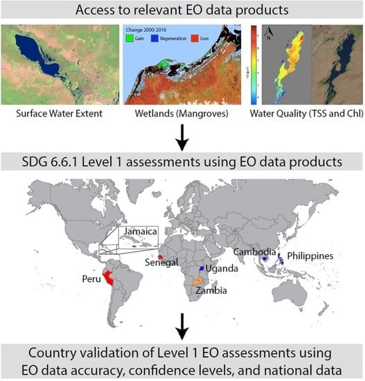
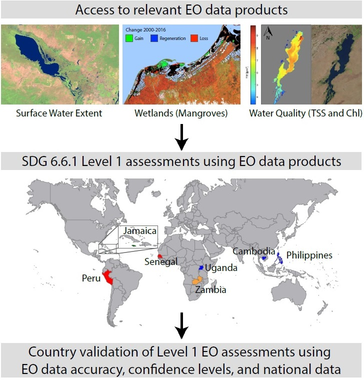
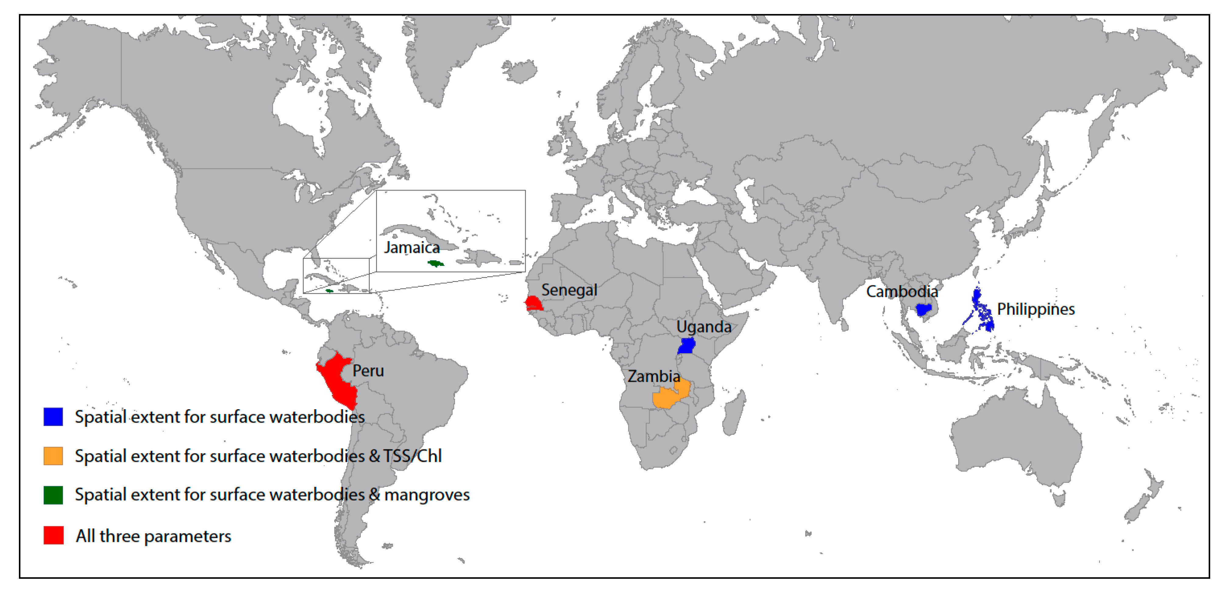
2. Overview of the Study

Global monitoring of SDG 6 was initiated in early 2017 following development, testing, and evaluation of methodologies for monitoring the associated indicators. The UN Environment is the custodian agency for SDG Indicator 6.6.1 and developed a step-by-step methodology that explains how to monitor the sub-indicators (further broken down into categories and components), including definitions, computational steps, and recommendations on spatial and temporal resolutions. Custodian agencies are charged with producing methodologies for collecting data from national data sources and tracking progress, as well as contributing to statistical capacity building, among other key activities. The UN Environment, in collaboration with the Group on Earth Observations (GEO) and space and research agencies including the National Aeronautics and Space Administration (NASA), the European Space Agency (ESA), and the Joint Research Centre (JRC), are working to support the use of EO for Indicator 6.6.1 data collection and reporting. To support this effort, we explored how and to what extent readily available EO data products and emerging tools could help countries report on this indicator. Seven pilot countries were included in the study based on input from the UN Environment and formal agreement from the countries to participate in the pilot study based on their interest in using EO data and conducting future ground-based validation studies. Figure 1 shows the location of the seven countries considered in this study and the corresponding components that were investigated for each country.
Table 1 provides a summary of the reporting requirements for this indicator based on the 2018 monitoring methodology for SDG Indicator 6.6.1 [46] and the components and categories considered in this study. The UN Environment has adopted a progressive two-level monitoring approach for Indicator 6.6.1. Level 1, which includes the spatial extent of water-related ecosystems and water quality (only Chl and TSS) of lakes and artificial water bodies, is based on globally available data from EO and is reviewed by countries every five years. During the review process, countries can either accept, reject, modify, or replace the EO data provided by the UN Environment. Level 2, which includes the quantity of water (discharge) in rivers and estuaries, water quality, and quantity of groundwater within aquifers, is based on available national data from each country. In this study, we only considered Level 1 monitoring, with one exception of only considering mangroves among the vegetated wetlands. The water-related ecosystem category of vegetated wetlands in SDG Indicator 6.6.1 includes swamps, fens, peatlands, marshes, paddies, and mangroves. Considering multiple types of wetlands would have added complexity to the study and we believe detracted from the central goal of having a multi-disciplinary proof of concept to guide future work on the use of EO data for Indicator 6.6.1 reporting. This decision was also made because mangroves are especially vulnerable and unique ecosystems that exist at the boundary between freshwater and seawater and are globally not mapped and monitored in a consistent and reproducible manner. Mangroves provide important ecosystem services for many countries such as helping to remove pollutants from water, serving as a buffer against storm surge, providing protection from coastal hazards [47,48], and providing economical blue carbon benefits [49]. More so, the flat coastal topography and forested nature of these ecosystems allow for remote sensing classification methods that can better separate mangroves from other herbaceous wetland types.
It is noted that although this study extracts national statistics for the components investigated, we present these numbers solely for demonstrative purposes and are in no way providing them so that they are used as official country statistics. As is the case for all of the SDG indicators, SDG Indicator 6.6.1 reported values only come from countries themselves, following a robust validation process.

3. Methodology

In this study, we followed the UN Environment Indicator 6.6.1 methodology using only readily available EO data based on two criteria. First, we limited the study to satellite-based EO data that are available for free and easily accessed through existing data sharing platforms. Next, we focused on data products and methodologies where there is a growing trend of more user-friendly data sharing platforms stemming from end-user community demands. All of the surface water data products and the water quality data can be accessed via a dedicated data sharing platform. A platform for the mangroves data is currently under development. Table 2 provides a summary of the datasets used for each of the water-related ecosystem categories and components considered in this study. Section 3.1, Section 3.2 and Section 3.3 provide more detailed information about the datasets and methodologies used to measure and/or evaluate the components.

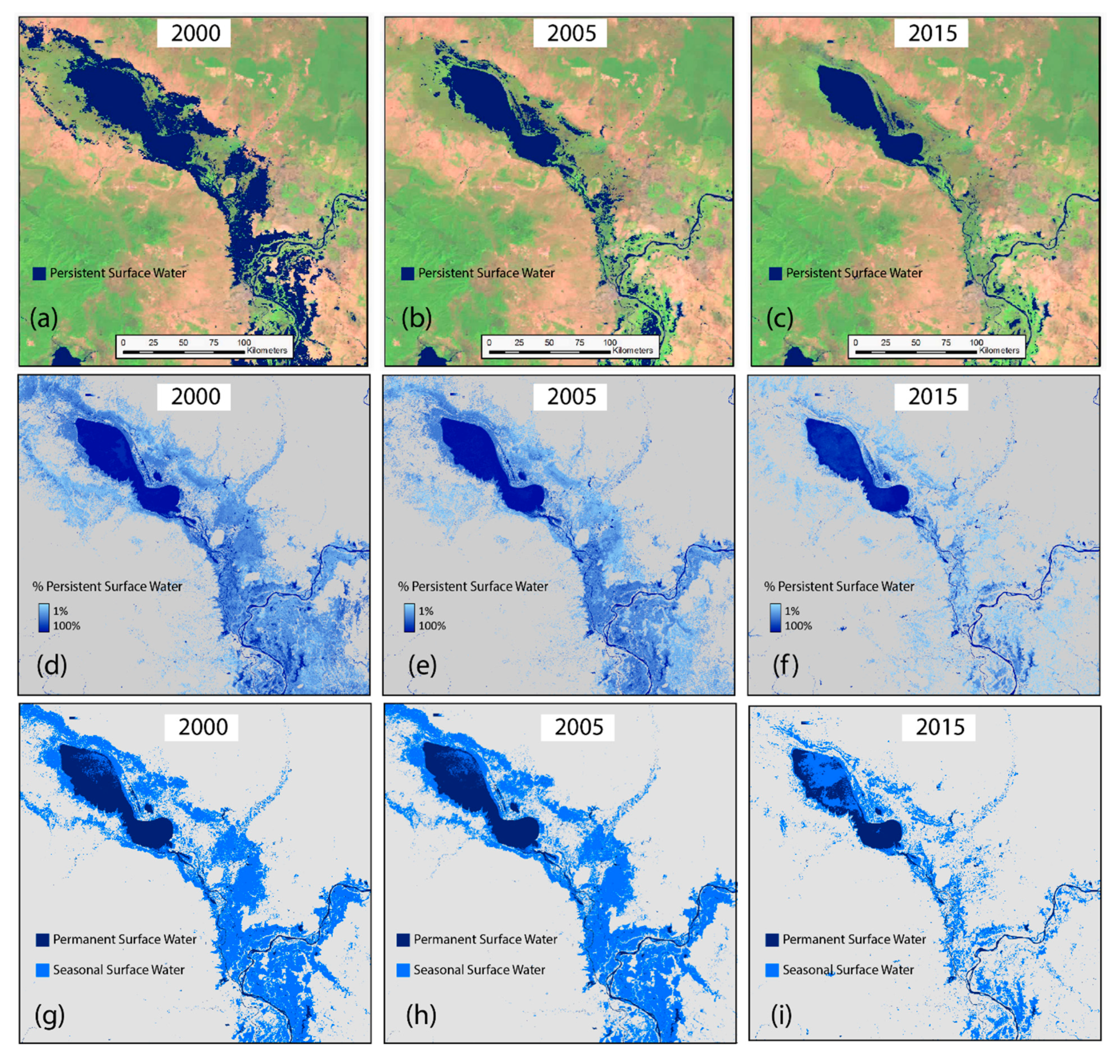
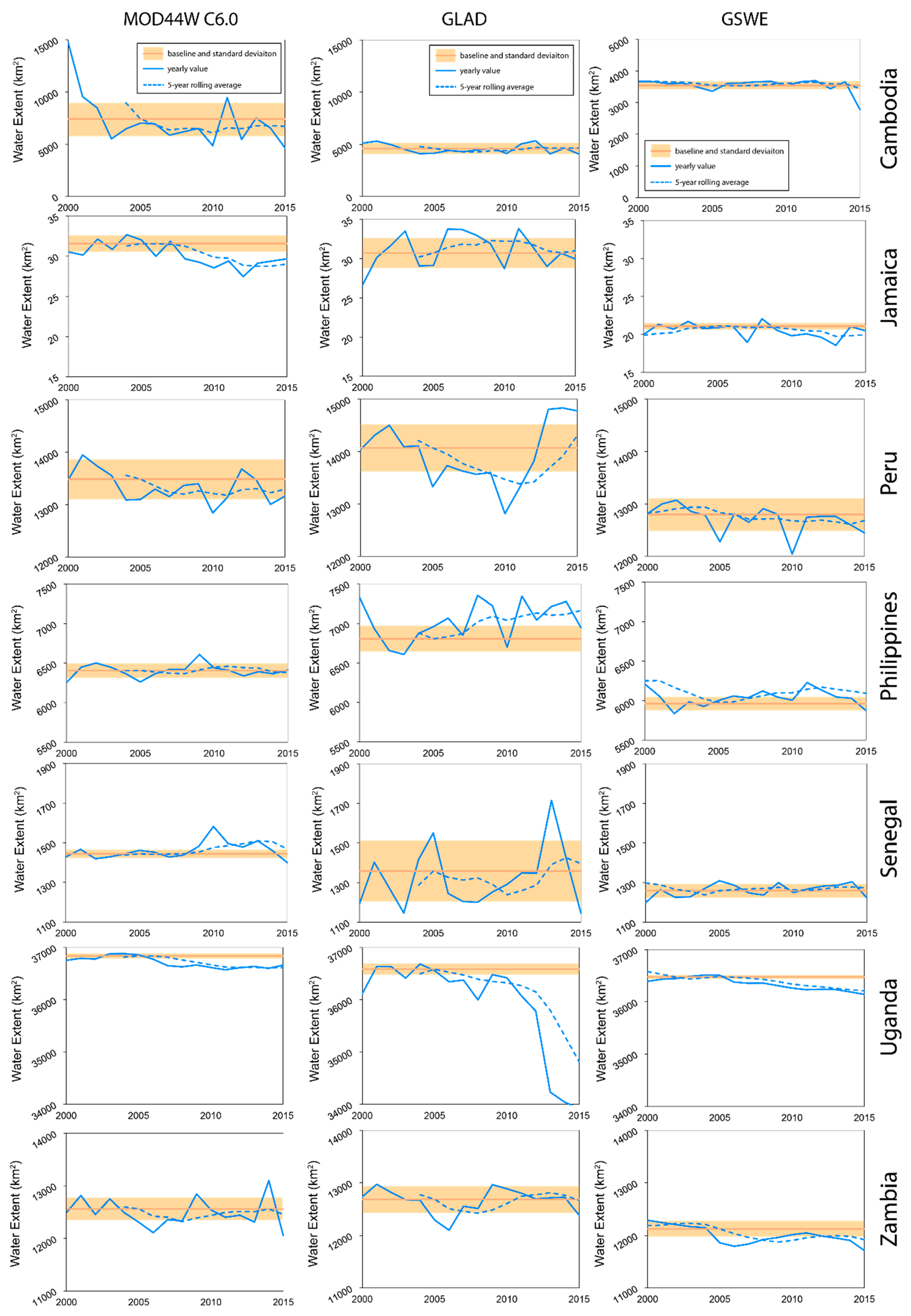
3.1. Spatial Extent of Surface Water Bodies

Three readily available satellite-based global surface water data products were used in this study. Data from MOD44W C6.0, Global Land Analysis and Discovery (GLAD) Surface Water, and JRC Global Surface Water Explorer (GSWE) were used to map and measure surface water extent from 2000 to 2015 for the seven pilot countries. The total area of surface water extent for each country was nationally aggregated using the United Nations Food and Agriculture Organization Global Administrative Unit Layers (GAUL) for 2000 to 2015. A baseline period of 2001 to 2005 was used, over which the data were averaged and compared, in alignment with the 2018 Indicator 6.6.1 monitoring methodology. Comparisons were done by calculating the Pearson correlation coefficients between the different data products; significance was determined with a p-value of ≤0.05 using the t-test. Yearly estimates of surface water extent and five-year rolling averages were compared with the 2001 to 2005 baseline period average and standard deviation. The five-year rolling averages were considered for 2004 to 2015 because MOD44W C6.0 data were not available before 2000 and GLAD data were not available before 1999. Using the three different data products and the methodology described, we investigated (1) the influence of water threshold definition on country aggregates of surface water extent (i.e., the number of observations or months per year that were classified as water in each pixel), (2) interannual deviations from the baseline period, and (3) considerations for countries when using any of the three data products. Section 3.1.1 and Section 3.1.2 provide an overview of each data product.

3.1.1. MODIS-based MOD44W C6.0

MOD44W C6.0 [50] is a collection of global water maps created on an annual basis from data retrieved by the MODIS instrument onboard the Terra satellite; it was created as an extension of the older MOD44W C5 water mask [51]. The MOD44W C6.0 data product has a spatial resolution of 250 m. MOD44W C6.0 is available for each year from 2000 through 2015 and for every major land mass (excluding Antarctica).
MOD44W C6.0 uses the MOD44W C5 water mask as the base to create annual summaries of water observations. All daily MODIS surface reflectance images for each year are classified into maps of water/not water by a decision tree algorithm, originally described by Carroll et al. [51]. A series of masks are applied to address known issues caused by terrain shadow, burn scars, cloudiness, or ice cover in oceans. These daily maps are then composited together for each year to make a single annual water map, using the definition that a pixel is considered persistent water for the year if it was water in at least 50% of the valid observations for that year. This is done separately for each year of data, from 2000 through 2015. The MOD44W algorithm was validated in the US with an existing water map from the National Land Cover Dataset as described by Carroll et al. [51]. In addition, extensive but not statistically comprehensive manual spot-checking and quality assurance was performed for revision by Carroll et al. [50].

3.1.2. Landsat-based GLAD Surface Water

The GLAD surface water dataset [52] was created through automated process mining of the entire 1999 to 2018 archive of the Landsat 5 Thematic Mapper (TM), the Landsat 7 Enhanced Thematic Mapper-plus (ETM+), and the Landsat 8 Operational Land Imager (OLI) by the University of Maryland’s GLAD Lab as part of a global study. The GLAD data product has a spatial resolution of 30 m. Water, land, and bad data classification models developed for each Landsat sensor at the University of Maryland and described by Potapov et al. [53] were applied to all 1999–2018 Landsat scenes using Google Earth Engine. A total of 80,345 scenes was classified for the seven countries in this study from 2000 to 2015.
A brief description of the GLAD data product is provided. After conversion to top of atmosphere (TOA) reflectance, the Landsat 5, 7, and 8 scenes were classified per pixel into land, water, cloud, shadow, haze, and snow and ice via per-sensor, hierarchical, bagged classification trees utilizing all of the available image bands, normalized difference ratios of each pair of spectral bands, and 3 × 3 pixel spatial averages of all bands and ratios. Elevation and derived slope, aspect, and hillshade data were used as additional metrics and obtained from the Shuttle Radar Topography Mission (SRTM). The classification trees were built using a global training set of 120 to 160 fully classified scenes per sensor. The land and water observations for a given pixel were summed per month, measured by the percent of clear observations flagged as water, and aggregated to annual water presence frequency. For this study, the GLAD data were run using three different thresholds for persistent water, including the presence of water in at least 50%, 75%, and 90% of the valid observations for a given year, respectively. These thresholds were selected to explore the influence of the persistent water definition on national level water accounting and to demonstrate the importance of this definition when using EO-based surface water data. The monthly maps have users’ and producers’ accuracies of 93.7% (±1.5%) and 96.0% (±1.2%) when thresholded at 50% and compared against 5 m reference data. Pickens et al. [52] provide a full validation and description of the methodology of the GLAD surface water dataset.

3.1.3. Landsat-based Global Surface Water Explorer

Surface water estimates from the 30 m spatial resolution GSWE data [15] were also used in this study. The UN Environment recently endorsed the use of GSWE data for country reporting and the dataset is part of a special SDG 6.6.1 online data portal developed jointly by the JRC, Google, and UN Environment. Similar to GLAD Surface Water, GSWE uses the entire archive of the Landsat 5 TM, the Landsat 7 ETM+, and the Landsat 8 OLI orthorectified, TOA reflectance, and brightness temperature images acquired from 16 March 1984 to present. Pekel et al. [15] provide a full description of the GSWE methodology. The GSWE yearly permanent and seasonal surface water and five-year rolling average permanent surface water data were accessed for the seven countries via the SDG Indicator 6.6.1 data portal. GSWE data define permanent water as surfaces that are under water for all months of a year, and seasonal water as surfaces with water one to 11 months of a year, based on available Landsat imagery. In this study, the term “seasonal” data is used to represent the combined permanent plus seasonal GSWE data, which is in better alignment with the other two data products.

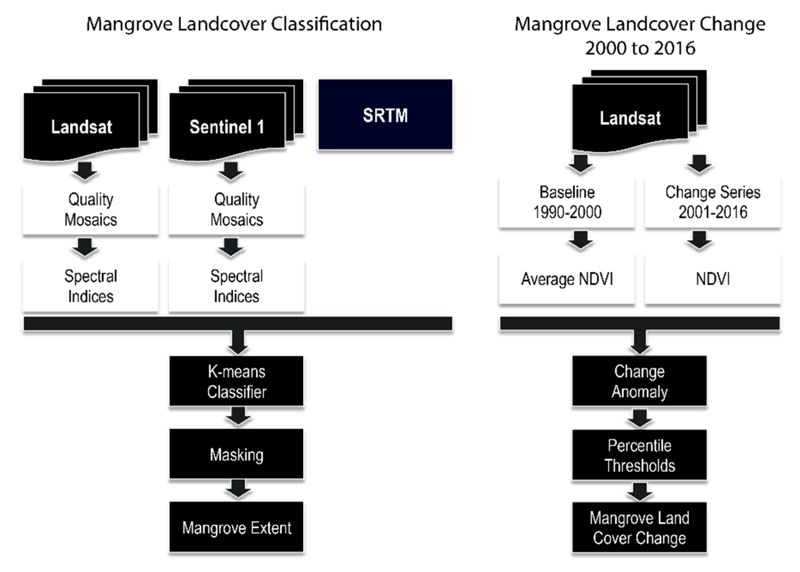
3.2. Spatial Extent of Mangroves

We used a combination of satellite imagery sources to develop a semiautomatic approach to measure the extent and change of mangrove wetlands in Jamaica, Peru, and Senegal. The data consisted of Landsat 8 OLI, Sentinel-1, and SRTM elevation data. Landsat data were pre-processed by image resampling, conversion to TOA reflectance, cloud and shadow removal and quality assessment, and image normalization. Landsat 8 OLI bands were used as inputs for the classification, as well as the normalized band ratios Normalized Difference Vegetation Index (NDVI), Normalized Water Index (NWI), Normalized Burn Ratio (NBR), and others outlined by Green et al. [54]. Additionally, annual maximum ‘VV’ and ‘VH’ metrics from Sentinel-1 and elevation data from SRTM were resampled and included in the classification. Areas where SRTM elevation was over 50 m and areas where the annual maximum NDVI values were less than 0 were masked out prior to analysis to improve the classification. By doing this, areas where the elevation was too high or areas of permanent water bodies were removed, respectively. A K-means clustering algorithm was used to generate 60 land cover types using 10,000 randomly sampled points within the area of analysis. Automatic detection of the land cover types was then merged into mangrove and non-mangrove classes using visual interpretation of the annual 2016 Landsat composite. Google Earth imagery was used extensively as an additional reference for the 2016 classification.
A NDVI anomaly was calculated for each study region using the Landsat image archives following similar methods outlined by Lagomasino et al. [55]. The reference period covered Landsat 5 TM images from January 1990 through December 1999. Images were pre-processed following a similar criterion as the mangrove extent. A mean NDVI value was generated from the sum of individual pixels across all images that were normalized by the number of images representing non-null values. The mean NDVI for the reference period (1990 to 2000) was then subtracted from each of the images in the observation period, which ranged from January 2000 to December 2016. The anomaly value from each overlapping pixel was then summed across all of the images in the collection to determine an overall cumulative anomaly. The cumulative anomaly values were also normalized for the total number of images with non-null values for individual pixels. Anomalous NDVI values were considered those which fell outside the 5th and 95th percentiles over the study region [55]. Values greater than the 95th percentile were considered areas of forest gain, while those values less than the 5th percentile were characterized as forested areas that were lost. Gains in mangrove area from 2000 to 2016 were assumed to only occur within the 2016 extent as mapped for this study. Conversely, any loss during the 16-year period was assumed to only occur within the mangrove extent in 2000 as mapped by Giri et al. [25]. The mangrove extent maps for 2000 and 2016 were used to mask regions of losses and gains, respectively, from the NDVI anomaly. Figure 2 provides a schematic of this methodology. National level statistics were obtained for all three countries using the Food and Agriculture Organization (FAO) GAUL administrative boundary dataset.

3.3. Water Quality of Surface Water Bodies

While EO provide a full suite of water quality products, including Chl, TSS, colored dissolved organic matter (CDOM), turbidity, Secchi depth, and surface temperature, in this study, we focused on Chl and TSS (following UN reporting requirements for Level 1) derived using best-practice empirical algorithms in different lake systems in Zambia, Peru, and Senegal. The TSS algorithm uses information in the red spectral bands [56], and the Chl retrieval is based on the heritage ocean color algorithm [57], which uses the band ratio of green-blue bands. Relevant bands from the Landsat 8 and Sentinel-2A/B images were processed using NASA’s SeaWiFS Data Analysis System (SeaDAS) whose performance has been evaluated and well documented [58,59]. SeaDAS removes and/or minimizes the impacts of interfering atmosphere using a heritage atmospheric correction algorithm [60] developed originally for ocean color. The atmospherically corrected spectral reflectance just above the water surface is then applied to derive Chl and TSS. The relative differences in the above-water reflectance products as well as in the TSS products derived from Landsat and Sentinel-2 images processed via SeaDAS have recently been identified and minimized to enable seamless analysis of global surface water quality [61]. The utility of the combined products, however, have not been thoroughly assessed for societal benefits (e.g., SDG reporting). To this end, five surface water bodies located in three different countries were evaluated in this study: Lake Bangweulu in Zambia, Lake Titicaca and Lake Junin in Peru, and Casamance River and Lake Guiers in Senegal. We report area-average Chl and TSS over time, starting from April 2013 when Landsat-8 became operational. The analysis only focuses on the relative variations in Landsat and Sentinel-2 derived products, thus an assessment of the precision and accuracy of Chl and TSS was considered beyond the scope of this proof of concept study.

4. Results

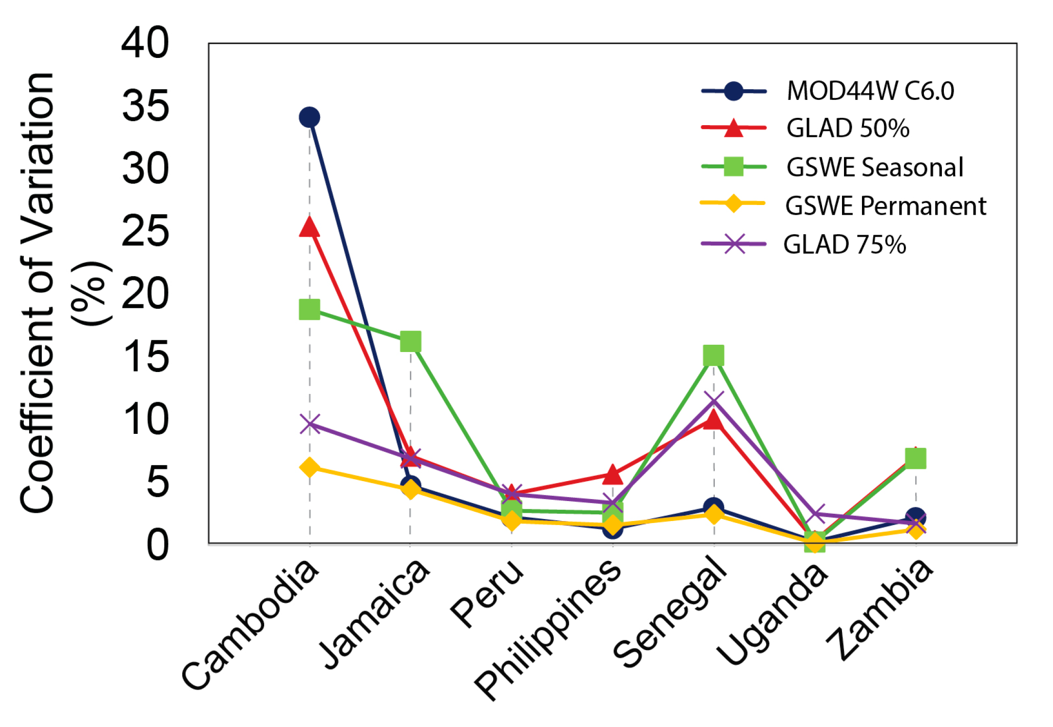
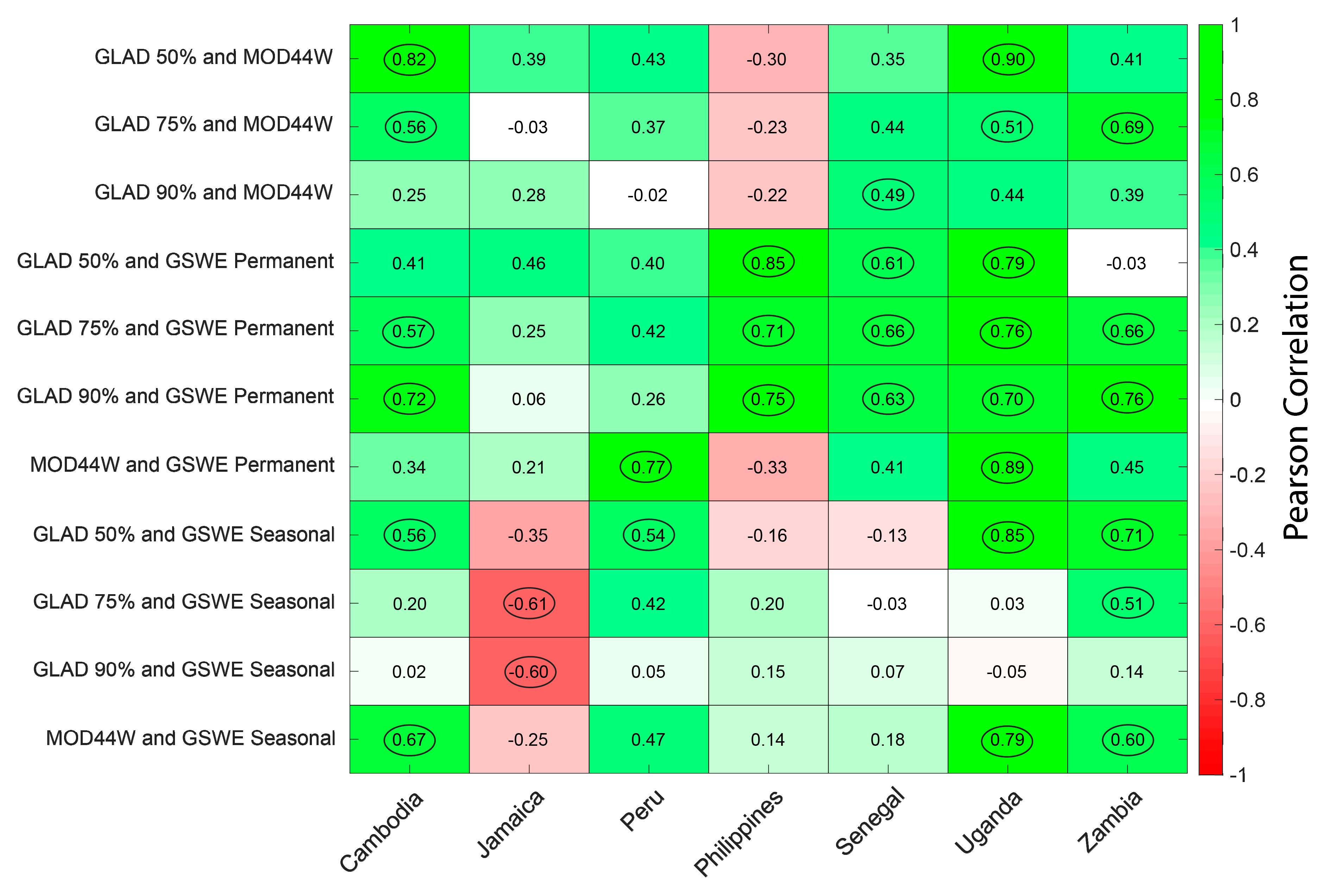
4.1. Spatial Extent of Surface Water Bodies

Many of the differences between the surface water data products exist due to the threshold definition for persistent, permanent, or seasonal water used by the particular EO-based surface water data product. In this study, we used the set threshold definitions for MOD44W C6.0 and GSWE data products, as discussed in Section 3.1. However, with the GLAD data we were able to explore different persistent water thresholds. To illustrate this concept, Figure 3 provides an example of the spatial extent of surface water for the Tonle Sap Lake in Cambodia mapped with the three data products for three of the years in the study period, with 2000 being exceptionally flooded due to a series of tropical storms and heavy monsoon rains that occurred during that year, 2005 being relatively average, and 2015 being the driest year of the 16-year record considered in the study. Much of what was considered seasonal water with GSWE in 2000 (thus not accounted for in the permanent water data) was considered persistent water in the MOD44W C6.0 data product because the pixels were flooded in more than half of the valid observations during that year. The surface water extent in 2000 for Cambodia was 14,753 km2 with MOD44W C6.0, 18,269 km2 with the GSWE seasonal data, and 11,834 km2 with the GLAD 50% persistent water threshold. The slightly lower value with GLAD data can be explained by the fewer number of observations with Landsat vs. MODIS due to cloud cover during the 2000 storms and monsoons and the higher chance for MOD44W C6.0 to have valid observations during these times due to the daily revisit time of MODIS. The slightly higher value with GSWE data can be explained by the seasonal water threshold definition used, which includes any valid pixel that is classified as water for one to 11 months in a year. In 2015, the driest year during the record, the yearly aggregate surface water extent was 4645 km2 with MOD44W C6.0, 10,632 km2 with GSWE seasonal data (3355 km2 with GSWE permanent data), and 5317 km2 with the GLAD 50% water threshold (3568 km2 with the GLAD 90% water threshold). Due to the higher spatial resolution of Landsat vs. MODIS, Landsat-based data are able to capture smaller water bodies that may otherwise be missed by MODIS, thus during years when cloud cover is not a significant issue, Landsat-based estimates of surface water will likely be higher than MODIS-based estimates, as illustrated here.
Figure 4 shows the yearly and five-year rolling average variability in surface water extent, compared to the baseline average and standard deviation of the baseline average. For brevity, only the GLAD surface water 75% threshold and GSWE permanent surface water data are displayed. The greatest number of years where the yearly data were outside the baseline average and standard deviation occurred in Uganda, where there was a distinct downward trend beginning from 2006 to 2010/2011. However, with the exception of the GLAD data, all deviations were within less than 2% of the baseline. Deviations for the last three years of record from the GLAD data were between 6% to 7%. Even after the five-year moving average smoothing, more than half of the years during this period were outside of the baseline standard deviation with all three datasets. This decline in surface water extent aligned with a decline in East African rains attributed to multi-decadal variability in the Indian Ocean sea surface temperatures, resulting in a prolonged period of drought in the region and culminating in the worst drought experienced in decades during 2010/2011 [62,63]. Several other countries, the Philippines in particular, had five or more years where the annual spatial water extent exceeded the baseline period variance. The GSWE permanent baseline value was in all cases lower than all other data products, which was to be expected.
The coefficient of variation, which is a standardized measure of dispersion, was calculated to explore interannual variability in surface water extent (Figure 5). Generally, all of the datasets had a similar coefficient of variation. The countries with the highest coefficient of variation—Cambodia, Jamaica, and Senegal—also exhibited the greatest differences in the coefficient of variation between the datasets. This finding was as expected. One finding that was unexpected, however, was that besides Cambodia, MOD44W C6.0 and the GSWE permanent data exhibited similar coefficients of variation despite countries such as Jamaica, the Philippines, and Senegal exhibiting greater variability with more seasonal datasets. This is either due to the ability of the MOD44W C6.0 data to classify persistent water based on more MODIS scenes per year or due to the lower spatial resolution of these data, which may not account for seasonal variability of smaller water bodies.
The GLAD and GSWE permanent water data were generally strongly correlated, particularly when comparing the GLAD 75% and 90% persistent water data with the GSWE permanent water data (Figure 6). Since both data products are Landsat-based, this was an expected result. Given the threshold used to define permanent water by GSWE, we expected that the higher persistent water thresholds for the GLAD data would result in greater agreement. The opposite relationship was expected for the GSWE seasonal data. For Cambodia, Peru, Uganda, and Zambia this was the case— there were statistically significant correlations between the GLAD 50% persistent water data and the GSWE seasonal water data but not with the other two GLAD persistent water thresholds (the exception was a statistically significant, although relatively low, correlation between the GLAD 75% persistent water data and the GSWE seasonal water data in Zambia). With the exception of Jamaica and the Philippines, there was generally good agreement between GLAD 50% and 75% and MOD44W C6.0 and GSWE permanent and MOD44W C6.0.
Uganda, Cambodia, and Zambia had the highest number of statistically significant correlations between the six datasets. The highest level of agreement was in Uganda, where the average correlation was 0.6 overall and 0.75 among the GSWE permanent water and the three GLAD persistent water datasets (Figure 6). The majority of these correlations were statically significant. Jamaica was the only country to have a significant negative correlation when comparing the GSWE seasonal data with the other datasets considered, although non-significant negative correlations were also notable for the Philippines. As the only two island nations in the study, the negative correlations for Jamaica and the Philippines were attributed to the nature of seasonal surface water classification along the coasts. Since the GSWE seasonal data account for persistent water anywhere from one to 11 months, these yearly estimates included short-term seasonal flooding that the other datasets did not.

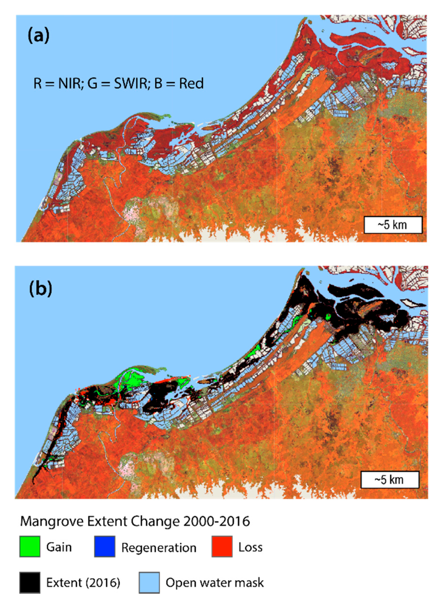
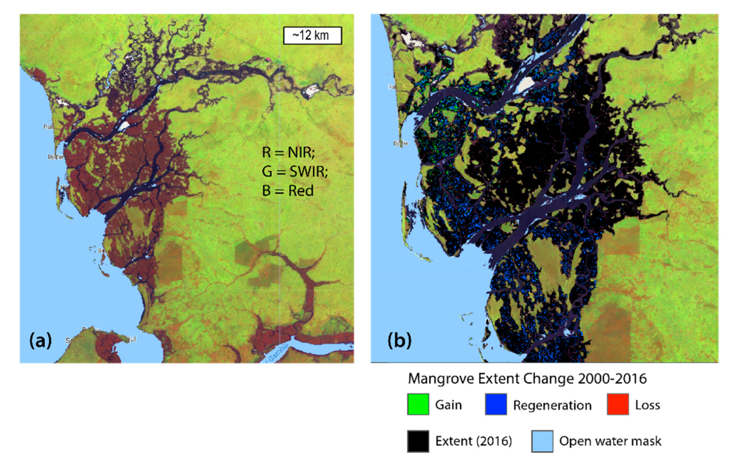
4.2. Spatial Extent of Mangroves

Table 3 provides the area corrected change in mangrove extent for the three study countries and associated uncertainties based on reference data and the accuracy assessment error matrix [64]. These area corrections and uncertainties take into consideration the errors associated with the classification to provide a more realistic estimate of mangrove cover and change over just “pixel-counting”. From 2000 to 2016, Senegal and Peru had a net gain in mangrove extent while Jamaica had a net loss. Jamaica also experienced the greatest uncertainties in estimated extents, with uncertainty for mangrove gain during this period being as high as ±32% and uncertainty for mangrove loss being as high as ±21%. On average, uncertainty was higher when estimating mangrove gains vs. mangrove losses, partially because these areas were higher overall. However, Jamaica was the exception to this, where the mangrove gain area was less than the loss, yet the associated uncertainty was still relatively higher.
It was beyond the scope of this study to investigate the reasons behind the changes presented in Table 3, as the monitoring methodology for SDG Indicator 6.6.1 currently does not require this information to be reported. However, the land cover change data allowed us to look more closely at the estimated changes. In Figure 7 and Figure 8 we show example maps for a mangrove region in Peru and Senegal, respectively. These figures provide a sub-national look at the type of mangrove forest gain experienced by the countries. For example, most of the additional mangrove area increase between 2000 and 2016 in the Tumbes District of Peru was due to mangrove gain, defined as the expansion of mangrove to previously uninhabited areas (e.g., open water to mangrove or bare soil to mangrove, see Figure 7). This took place in localized hotspots along the coast. Conversely, most of the additional mangrove area increase between 2000 and 2016 in the Kaolack Region of Senegal was due to the expansion of mangroves into mudflats (Figure 8). Though not explicitly detailed in Indicator 6.6.1, we were also able to monitor areas of regeneration, here defined as the increase in vegetation signal in areas that were previously identified as mangroves [25], which represent varying degrees of regrowth. This expansion and regeneration are reflective of large mangrove reforestation projects in the Senegambia region, where between 2006 and 2013 it was estimated that 14,000 ha of mangrove forest were replanted [65]; with 79 million mangroves replanted it, is considered the world’s largest mangrove reforestation project [66].

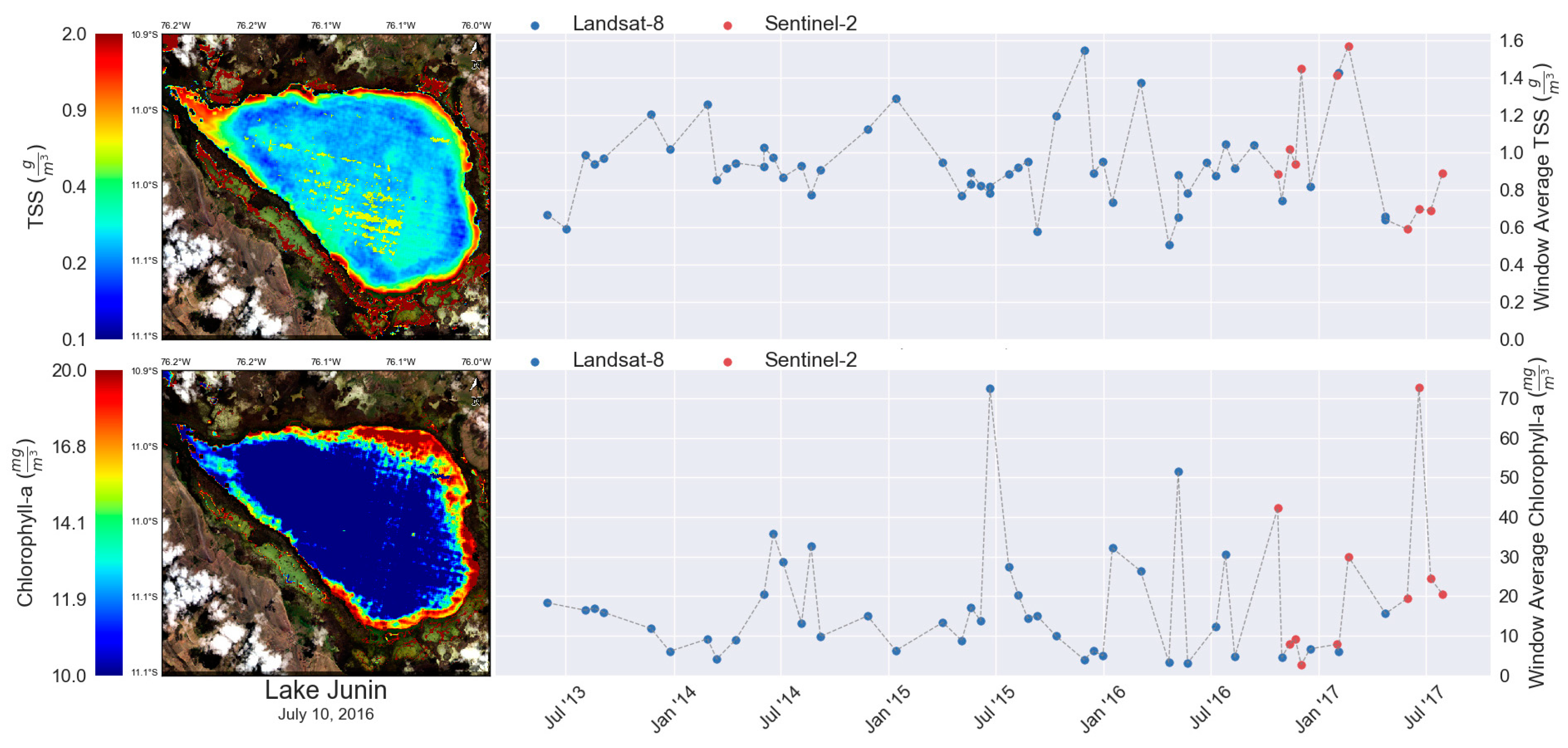
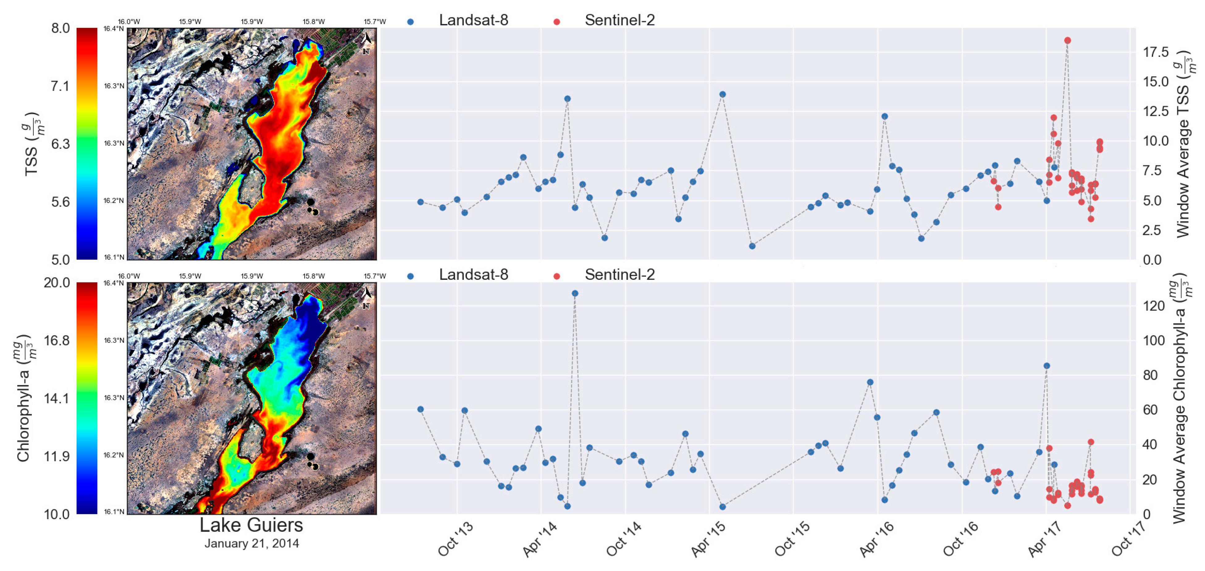
4.3. Water Quality of Surface Water Bodies

The time-series (2013–2017) of water quality indicators for select large water bodies is shown in Figure 9, Figure 10, Figure 11, Figure 12 and Figure 13. The temporal analyses begin in 2013 (earliest) and are shown alongside an example distribution of TSS and Chl products (left). The datapoints in the temporal plots indicate area-average Landsat 8 or Sentinel-2A/B-derived TSS and Chl products given in units of g/m3 and mg/m3, respectively. Although the frequency of observations is limited both by satellite revisit times and cloud cover, the variability in average water quality in different water bodies can be inferred. It is noted that these plots were only produced to support the proof of concept for how satellite-derived TSS and Chl may be used to inform countries in their Indicator 6.6.1 reporting. The aim of this effort was not to explain the mechanisms (also not required for Indicator 6.6.1 reporting) that may have led to certain anomalies or trends, and any future application of the methods described would require robust validation and characterization of the uncertainties.
In Lake Junin (Figure 9) Chl anomalies were identified in July 2015 and 2017, although lake-wide TSS values varied only slightly in time with no distinct peaks. Lake Titicaca (Figure 10) displayed more distinct peaks in TSS, with anomalies in TSS most noticeable in November 2015 and 2016. Sentinel-2 data also captured a major peak in August 2017 where Chl was nearly 25 times higher than the time-averaged concentration (2013–2017). High concentrations of TSS and Chl were revealed by Landsat data in April and May of 2014 in Lake Guiers (Figure 11). Data gaps due to cloud coverage during several months in 2015 inhibited us from having valid observations during those times, however, the addition of Sentinel-2 data beginning in 2017 considerably increased our observation rate at this site. TSS and Chl variability in the Casamance River were relatively consistent during the study period (Figure 12). For Lake Bagweulu (Figure 13), clear seasonal patterns in TSS with different peaks in September and October timeframes were inferred, while high-frequency variations in Chl during May to September were identified and a major peak in Chl was captured with the Sentinel-2 data during late March 2016.

5. Discussion

Although we considered three different data products and six datasets for surface water, including GSWE permanent and seasonal data which are already endorsed by the UN Environment, it is difficult to draw conclusions on the best product for all countries to use in their reporting without in-country validation. Overall, we found there to be greater agreement between the six datasets for the landlocked countries than for the non-landlocked countries, and we found the least agreement for the two island nations. Further investigation using a greater number of countries than were considered in this study is needed to verify this trend. Where there was poor agreement between datasets, we attributed the majority of the differences to three things: (1) each uses a slightly different threshold definition and methodology for calculating persistent, or in the case of GSWE, permanent water; (2) MOD44W C6.0 maps, with the daily repeat coverage of MODIS, have a higher likelihood of accurately measuring surface water extent in areas with limited Landsat observations due to cloud cover (together Landsat 7 and 8 image the globe once every eight days); and (3) the two Landsat-based data products were able to resolve much smaller features than the MODIS-based MOD44W C6.0 dataset given their higher spatial resolution. There are also some additional nuances when it comes to threshold definitions for EO-based surface water extent that would be important for countries to note when using these types of data to support SDG reporting. MOD44W C6.0 and GLAD both define surface water based on the percentage of valid observations during each year where persistent water is detected. GSWE defines surface water based on the number of months per year where persistent water is detected from valid observations. In some cases, valid observations may not be available due to gaps in the Landsat record or omitted observations (considered invalid) due to cloud cover and/or other obstructions (e.g., trees or shrublands). These nuances can result in discrepancies between data products for certain geographical regions during certain years, stressing the need for countries to conduct rigorous in-country validation of the EO-based data as part of reporting for SDG Indicator 6.6.1.
We identify the most important consideration in the practical application of EO-based surface water data for SDG reporting as the threshold definition for persistent or permanent water. This value is what ultimately accounts for surface water extent in each country, and as shown here it can vary greatly. In countries that experienced relatively little inter-annual and seasonal variability such as Uganda, Zambia, and Peru, we found relatively little difference in the coefficient of variation between the different datasets (Figure 5), although this did not necessarily lead to high correlations between the datasets (Figure 6). This provides some indication that in these countries any of the different datasets could provide a good basis for assessing relative change in surface water extent. However, in countries with a high degree of inter-annual and seasonal variability, such as Cambodia, Jamaica, the Philippines, and Senegal, deciding between datasets (e.g., permanent vs. seasonal) is more challenging. Since seasonal and inter-annual variability is an important part of the hydrological cycle in these countries, simply considering changes to permanent surface water extent may not be sufficiently capturing changes to their water-related ecosystems. We argue that these countries may benefit from selecting a seasonal threshold for persistent water based on national and regional hydrological regimes and ground-based validation, rather than using a consistent definition.
The inter-comparison and determination of some degree of statistical agreement between different datasets, as illustrated in this study, can be used to provide confidence levels for the surface water extent Level 1 data, which would be helpful for national-level decision-making during the Level 1 country validation process (i.e., deciding whether to accept, reject, modify, or replace the data provided). Additionally, while any EO-based data product would require rigorous validation before being used for SDG reporting, the inter-comparison between similar data products can also supplement ground-based validation studies where resources are otherwise limited. In such cases, since all of the datasets considered in this study are geospatially mapped, countries could target ground-based validation efforts where the greatest spatial differences between datasets exist.
Another important consideration for the use of EO-based surface water extent data for SDG Indicator 6.6.1 reporting is the baseline period. For some of the countries in this study, the baseline period from 2001 to 2005 seemed sufficient in capturing the inter-annual variability, especially when using the five-year rolling average annual data. However, in the case of countries such as Cambodia, Jamaica, the Philippines, and Uganda, where several years within the study period appeared to be anomalously wet or anomalously dry years (in comparison to the baseline period), the baseline period and variance may need to be modified. For example, although Uganda had the highest correlation among the data products, it also had the highest number of years that were outside of the baseline standard deviation (Figure 4). In most cases the deviation from the baseline amounted to less than 2%, however, this number was higher during the last years of record with the GLAD data.
Lastly, Landsat and MODIS surface water data products should only be used to study surface water bodies that are at minimum the length of several pixels in each dimension. While Landsat data can resolve much smaller water bodies than MODIS data, we note that even with a higher resolution Landsat-based data product, smaller water bodies such as rivers and streams and water bodies in forested areas may be missed, making supplemental data collection necessary. Regarding the use of different data products, it is also important that the same data product be used to track change from baseline values over time since baseline values can vary greatly between datasets as shown in this study. Even if several data products are used for inter-comparison, as suggested here, final reported values must be repeatable over time. Data and methodology consistency is needed to achieve this. If datasets are updated or changed, then the baseline and all other values would need to be recalculated.
In this study, we also combined different EO data (from different satellites and sensors) to estimate net changes in mangrove extent. Our results consider the challenges of directly comparing different spatial datasets, even with similar resolution, given the relatively high level of uncertainty with the mangrove change estimates (Table 3). We note that the data shared represent an average extent for each year and do not capture the highly dynamic nature of mangroves which at different times of the day or year can be submerged under water. We found the highest uncertainties with Jamaica which, along with findings from the surface water extent analysis, indicate that there may be more uncertainty when using EO data for small island nations that have smaller hydro-ecological surface features and where hydro-climatology can vary greatly over relatively small areas [67]. Supplemental land cover change data (as illustrated in our study) can provide information on the long-term trends in mangrove change, which would be important for informing management, investment, and policy change decisions. Trends of excessive gain or excessive loss can be useful in determining key locations for future restoration projects, such as those related to coastal resilience, in addition to helping countries meet their SDG reporting requirements for Indicator 6.6.1. It would be important for countries to account for the location of mangroves, the location where changes have occurred, the transitional state of change (e.g., open water to mangrove or bare soil to mangrove), as well as aggregate changes (gain vs. regeneration vs. loss). We argue that identifying the type of mangrove gain (or loss) is an especially critical piece of information for country reporting on SDG Indicator 6.6.1, and one that can easily be obtained via EO.
A key strength of using EO for SDGs is that the data are spatially exhaustive and provide global or near global coverage. However, there are also uncertainties involved with mapping land changes, such as for mangroves or other types of wetlands, using EO data. Errors can result from the change mapping process, the data used, and analyst biases [68]. Although change detection and mapping approaches using EO data are increasingly robust, any map made from satellite data can be assumed to contain some error, with the areas calculated from the map also potentially subject to bias. As illustrated in this study, an accuracy assessment is needed to identify the errors of the classification and the sample data in order to estimate both the accuracy and the uncertainty of the estimates. In this study, we used the good practices approach laid out by Olofsson et al. [64] to account for uncertainty in the estimates of mangrove area change over the study period. Land change accuracy assessment is separated into three major components: the response design, sampling design, and analysis. The response design encompasses all aspects of the protocol that lead to determining whether the map and reference classifications are in agreement. The sampling design is the protocol for selecting a subset of data within a region of interest. The analysis includes protocols for defining how to quantify accuracy along with the formulas and inference framework for estimating accuracy and area and quantifying uncertainty of these estimates. Conducting an accuracy assessment of a land change map serves multiple purposes and without one there is no way to communicate map quality in a quantitative and meaningful fashion. If EO data are used for national wetland reporting on Indicator 6.6.1, an accuracy assessment should also be done. Future guidance should include accuracy assessments as a criterion for country reporting using EO data.
Guidance for monitoring vegetated wetlands using EO data in support of SDG 6.6.1 reporting is still being developed and streamlined through global EO community efforts such as the GEO-Wetlands initiative, which aims to strengthen the cross-cutting coordination of global wetland observations by involving key stakeholders on different levels, from different regions, and from all sectors in a user-needs driven framework. Contributions to existing mangroves monitoring and partnership initiatives such as the Global Mangrove Watch [69], Global Mangrove Alliance, and further development of emerging platforms such as the EcoMap Mangrove Vulnerability Monitoring Tool [70] are also part of this effort.
In addition to being able to map the spatial extent of select water-related ecosystems with EO data products, we demonstrate that trends in the water quality parameters of TSS and Chl in dry and wet seasons, and in winter and summer, can successfully be tracked using readily available satellite-based EO data products. We note that the limitation with using EO data to assess and report on water quality is that these data only provide information on concentrations of in-water materials that affect the color of water, such as TSS and Chl. However, Chl and TSS concentrations may be correlated with other important water quality parameters such as oxygen levels, pH, nutrients, or chemicals that are listed as targets under SDG sub-Indicator 6.3.2. For instance, high TSS in a water body can often mean higher concentrations of bacteria, nutrients, pesticides, and metals in the water that may indicate illegal discharges.
In this study, we showed that Landsat 8 and Sentinel-2 complement one another for TSS and Chl monitoring with several examples of Sentinel-2 data providing information, where cloud cover resulted in data gaps with the Landsat 8 instrument. While the uncertainties in the satellite products used are not quantified here, there are ongoing efforts with the UN Environment to develop close collaborations and engagements with a number of pilot countries in order to investigate the extent to which these products could be used to support country reporting on SDG 6, based on field validation. This proof of concept study has fostered strong partnerships with a handful of countries (e.g., Peru) such that the corresponding water authorities have initiated coordinated field sampling and/or monitoring activities under satellite overpasses to enable a thorough evaluation of uncertainties in Chl and TSS products. These collaborations will further aid in advancing new science algorithms and methodologies for enhanced retrieval of Chl and TSS products. Moreover, we are investigating how EO data can help guide ground-based monitoring programs, thus enabling a more cost-effective means for the monitoring of water quality and helping to fill in some of the data gaps. In the future, NASA is planning to develop a satellite-based water quality warning system, which will also be used to support national water quality monitoring efforts and serve as a decision-support tool, helping countries identify the most critical water quality problems, while also reporting on relevant SDG indicators. During the development process, the system will be evaluated and tested for several bodies of water in various countries and contribute to the progressive monitoring of Indicator 6.6.1.
Regarding gaps for practical water quality monitoring with EO, space agencies and the aquatic remote sensing community should further explore innovative algorithms (e.g., algorithms based on optical water types [71] or machine learning) to enhance water quality products at regional and global scales and to seamlessly merge products obtained from various sources including in situ data. Combining various satellite assets will help overcome data scarcity over areas with frequent cloud cover, however, care must be taken to ensure consistency across all satellite observations and products. For example, blending products from Landsat, Sentinel-2, Sentinel-3, and Joint Polar Satellite System series will guarantee near-daily observations over larger bodies of waters (such as Lake Bangweulu); but it is still vital to ensure that all of these products are in agreement in order to enable consistent monitoring of SDG Indicator 6.6.1. We note that although our article focuses primarily on SDG Indicator 6.6.1, this proof of concept study and subsequent in-country validation efforts to quantify water quality parameters from space are also relevant for SDG Indicator 6.3.2, ‘Ambient water quality’, for which the UN Environment is also the custodian agency. Following this collaborative approach and future validation exercises, EO-based observables (such as Chl and TSS) can potentially be added to the list of SDG Indicator 6.3.2 parameters to allow for an operational use of EO products combined with in situ data in the future.

6. Conclusions and Recommendations

Based on findings from this study, we make the following conclusions and recommendations:
  • Statistically based comparisons between multiple EO surface water data products could be used to provide some degree of confidence for the Level 1 surface water extent data, which would help countries during the Level 1 validation process. Comparisons can also help target ground-based monitoring efforts, making validation efforts more cost-effective.
  • The ability to vary the threshold for persistent or permanent water would be beneficial for countries that experience a high degree of seasonality, as it is important to capture changes to seasonal water dynamics as well as permanent water.
  • Comparing annual or five-year average surface water extent to the baseline period of 2001 to 2005 may not correctly capture actual change in conditions for some countries that experience a high level of interannual variability as well as small islands such as Jamaica that have highly variable, yet relatively small, water and wetland features.
  • Mangroves are highly dynamic systems, thus it is important to account for the location of persistent mangroves, the location where changes have occurred, the transitional state of change (e.g., open water to mangrove or bare soil to mangrove), as well as aggregate changes (gain vs. regeneration vs. loss). All of these parameters can easily be quantified with EO data, as illustrated.
  • Identifying the type of aggregate mangrove change (gain vs. regeneration vs. loss) is an especially critical piece of information that can easily be obtained via EO data that we recommend is added to the monitoring methodology for SDG Indicator 6.6.1 in the future.
  • An accuracy assessment should be conducted and included with country reporting for Indicator 6.6.1 when using EO data to track changes to wetland extent.
  • Landsat 8 and Sentinel-2 satellite data can capture the spatial extent and seasonal changes of SDG water quality indicators of TSS and Chl in ways that ground-based monitoring cannot, which can make these EO products a great complement to existing ground-based monitoring campaigns. In other words, EO products should not replace ground-based monitoring activities.
  • TSS and Chl measurements via EO present a potentially significant opportunity for SDG 6 reporting, however, application of space-based water quality information will only be an asset if it is done in close collaboration with countries that can combine it with ground-based monitoring efforts and local information.
  • Data and methodology consistency is needed to achieve replicability over time, even if several different datasets are used. If datasets are updated or changed, then the baseline and all other values should be recalculated and resubmitted.
Space agencies and science institutions, in collaboration with the UN Environment, can help encourage the use of EO for water-related ecosystems monitoring in countries with currently limited data for reporting. Development and sustainable operation of open access web portals that enable easy data access, essential visualizations, basic statistical evaluations, integration with other data sources, capacity building through training, and clear communications on what can and cannot realistically be delivered with the use of EO data will be key aspects. Country-driven validation of the EO data products remains a priority to ensure successful EO data integration in support of SDG Indicator 6.6.1 reporting, yet it is important for users to understand the special nuances around EO data. The EO data analysis and statistical methods used in this study can be easily replicated for country-driven validation of EO data products in the future.

Author Contributions

Conceptualization, R.H., A.H., F.P., T.F., N.P., S.U., A.P., M.H. (Matthew Hansen), D.L., A.K., and D.W.; methodology, R.H., A.H., F.P., T.F., N.P., S.U., A.P., M.H. (Matthew Hansen), D.L., and D.W.; software, A.H., F.P., T.F., N.P., S.U., A.P., M.H. (Matthew Hansen), D.L., M.C., and B.S.; validation, A.H., F.P., T.F., N.P., S.U., A.P., M.H. (Matthew Hansen), D.L., M.C., and B.S.; formal analysis, R.H., A.H., F.P., T.F., N.P., S.U., A.P., M.H. (Matthew Hansen), D.L., M.C., and B.S.; investigation, R.H., A.H., F.P., T.F., N.P., S.U., A.P., M.H. (Matthew Hansen), and D.L.; resources, A.K., D.W., and S.S.U.; data curation, R.H., A.H., F.P., T.F., N.P., S.U., A.P., M.H. (Matthew Hansen), and D.L.; writing—original draft preparation, R.H., A.H., F.P., T.F., N.P., S.U., A.P., M.H. (Matthew Hansen), and D.L.; writing—review and editing, R.H., A.H., F.P., T.F., N.P., S.U., A.P., M.H. (Matthew Hansen), D.L., M.C., B.S., A.K., M.H. (Margaret Hurwitz), D.W., and S.S.U.; visualization, R.H., A.H., T.F., N.P., A.P., and D.L.; supervision, F.P., T.F., M.H. (Matthew Hansen), and N.P.; project administration, S.S.U.; funding acquisition, A.K., D.W., and S.S.U. All authors have read and agreed to the published version of the manuscript.

Funding

This work was supported and funded by the NASA Applied Science Program and United Nations Environment.

Acknowledgments

We acknowledge and thank Stuart Crane, Elisabeth Bernhardt, and Jillian Campbell from the United Nations Environment Freshwater Unit Ecosystem Division for their support of this work and very helpful feedback on the study and its findings.

Conflicts of Interest

The authors declare no conflicts of interest.

References

  1. United Nations. Sustainable Development Goal 6 Synthesis Report on Water and Sanitation; United Nations: New York, NY, USA, 2018. [Google Scholar]
  2. UN Environment. Progress on Water-Related Ecosystems—Piloting the Monitoring Methodology and Initial Findings for SDG Indicator 6.6.1; UN Environment: Nairobi, Kenya, 2018. [Google Scholar]
  3. Anderson, K.; Ryan, B.; Sonntag, W.; Kavvada, A.; Friedl, L. Earth observation in service of the 2030 Agenda for Sustainable Development. Geo-Spatial Inf. Sci. 2017, 20, 77–96. [Google Scholar] [CrossRef]
  4. Bogardi, J.J.; Dudgeon, D.; Lawford, R.; Flinkerbusch, E.; Meyn, A.; Pahl-Wostl, C.; Vielhauer, K.; Vörösmarty, C. Water security for a planet under pressure: Interconnected challenges of a changing world call for sustainable solutions. Curr. Opin. Environ. Sustain. 2012, 4, 35–43. [Google Scholar] [CrossRef]
  5. Jackson, R.B.; Carpenter, S.R.; Dahm, C.N.; Mcknight, D.M.; Naiman, R.J.; Postel, S.L.; Running, S.W. Water in a Changing World. Ecol. Appl. 2001, 11, 1027–1045. [Google Scholar] [CrossRef]
  6. Gleick, P.H. Global freshwater resources: Soft path solutions for the 21st century. Sci. Public Policy 2003, 302, 524–528. [Google Scholar] [CrossRef] [PubMed] [Green Version]
  7. Vörösmarty, C.J. Global water assessment and potential contributions from Earth Systems Science. Aquat. Sci. 2002, 64, 328–351. [Google Scholar] [CrossRef]
  8. Vörösmarty, C.J.; Green, P.; Salisbury, J.; Lammers, R.B. Global Water Resources: Vulnerability from Climate Change and Population Growth. Science 2000, 289, 284–289. [Google Scholar] [CrossRef] [Green Version]
  9. Davidson, N.C. How much wetland has the world lost? Long-term and recent trends in global wetland area. Mar. Freshw. Res. 2014, 65, 934–941. [Google Scholar] [CrossRef]
  10. Spalding, M.; Kainuma, M.; Collins, L. World Atlas of Mangroves; Earthscan: London, UK, 2010; ISBN 9781844076574. [Google Scholar]
  11. Michalak, A.M. Study role of climate change in extreme threats to water quality. Nature 2016, 535, 349–352. [Google Scholar] [CrossRef]
  12. ICSU/ISSC. Review of Targets for the Sustainable Development Goals: The Science Perspective; ICSU/ISSC: Paris, France, 2015; ISBN 9780930357979. [Google Scholar]
  13. Hák, T.; Janoušková, S.; Moldan, B. Sustainable Development Goals: A need for relevant indicators. Ecol. Indic. 2016, 60, 565–573. [Google Scholar] [CrossRef]
  14. Feng, M.; Sexton, J.O.; Channan, S.; Townshend, J.R. A global, high-resolution (30-m) inland water body dataset for 2000: First results of a topographic–spectral classification algorithm. Int. J. Digit. Earth 2016, 9, 113–133. [Google Scholar] [CrossRef] [Green Version]
  15. Pekel, J.; Cottam, A.; Gorelick, N.; Belward, A.S. High-resolution mapping of global surface water and its long-term changes. Nature 2016, 540, 418–422. [Google Scholar] [CrossRef] [PubMed]
  16. Mueller, N.; Lewis, A.; Roberts, D.; Ring, S.; Melrose, R.; Sixsmith, J.; Lymburner, L.; McIntyre, A.; Tan, P.; Curnow, S.; et al. Water observations from space: Mapping surface water from 25years of Landsat imagery across Australia. Remote Sens. Environ. 2016, 174, 341–352. [Google Scholar] [CrossRef] [Green Version]
  17. Tulbure, M.G.; Broich, M.; Stehman, S.V. Spatiotemporal dynamics of Surface water extent from three decades of seasonally continuous Landsat time series at subcontinental scale. Int. Arch. Photogramm. Remote Sens. Spat. Inf. Sci.—ISPRS Arch. 2016, 41, 403–404. [Google Scholar] [CrossRef]
  18. Tulbure, M.G.; Broich, M. Spatiotemporal dynamic of surface water bodies using Landsat time-series data from 1999 to 2011. ISPRS J. Photogramm. Remote Sens. 2013, 79, 44–52. [Google Scholar] [CrossRef]
  19. Fayne, J.V.; Bolten, J.D.; Doyle, C.S.; Fuhrmann, S.; Rice, M.T.; Houser, P.R.; Lakshmi, V. Flood mapping in the lower Mekong River Basin using daily MODIS observations. Int. J. Remote Sens. 2017, 38, 1737–1757. [Google Scholar] [CrossRef]
  20. Brakenridge, R.; Anderson, E. MODIS-based flood detection, mapping and measurement: The potential for operational hydrological applications. In Transboundary Floods: Reducing Risks Through Flood Management; Springer: Berlin/Heidelberg, Germany, 2006; pp. 1–12. [Google Scholar]
  21. Policelli, F.; Slayback, D.; Brakenridge, B.; Nigro, J.; Hubbard, A.; Zaitchik, B.; Carroll, M.; Jung, H. The NASA Global Flood Mapping System. In Remote Sensing of Hydrological Extremes; Lakshmi, V., Ed.; Springer: Berlin/Heidelberg, Germany, 2016; pp. 47–63. ISBN 978-3-319-43744-6. [Google Scholar]
  22. Huang, C. Detecting, Extracting, and Monitoring Surface Water From Space Using Optical Sensors: A Review. Rev. Geophys. 2018, 333–360. [Google Scholar] [CrossRef]
  23. Guo, M.; Li, J.; Sheng, C.; Xu, J.; Wu, L. A Review of Wetland Remote Sensing. Sensors 2017, 17, 777. [Google Scholar] [CrossRef] [Green Version]
  24. Fatoyinbo, T.E.; Simard, M. Height and biomass of mangroves in Africa from ICESat/GLAS and SRTM. Int. J. Remote Sens. 2013, 34, 668–681. [Google Scholar] [CrossRef]
  25. Giri, C.; Ochieng, E.; Tieszen, L.L.; Zhu, Z.; Singh, A.; Loveland, T.; Masek, J.; Duke, N. Status and distribution of mangrove forests of the world using earth observation satellite data. Glob. Ecol. Biogeogr. 2011, 20, 154–159. [Google Scholar] [CrossRef]
  26. Simard, M.; Fatoyinbo, T.; Smetanka, C.; Rivera-Monroy, V.; Castaneda-Moya, E.; Thomas, N.; Van der Stocken, T. Mangrove canopy height globally related to precipitation, temperature and cyclone frequency. Nat. Geosci. 2019, 12, 40–45. [Google Scholar] [CrossRef]
  27. Reilly, J.E.O.; Maritorena, S.; Mitchell, B.G.; Siegel, D.A.; Carder, K.L.; Garver, S.A.; Kahru, M.; Mcclain, C. Ocean color chlorophyll algorithms for SeaWiFS encompassing chlorophyll concentrations between. J. Geophys. Res. Ocean. 1998, 103, 24937–24953. [Google Scholar] [CrossRef] [Green Version]
  28. Doerffer, R.; Schiller, H. The MERIS Case 2 water algorithm. Int. J. Remote Sens. 2007, 28, 517–535. [Google Scholar] [CrossRef]
  29. Gerace, A.D.; Schott, J.R.; Nevins, R. Increased potential to monitor water quality in the near-shore environment with Landsat’ s next-generation satellite. J. Appl. Remote Sens. 2013, 7. [Google Scholar] [CrossRef] [Green Version]
  30. Keith, D.J.; Schaeffer, B.A.; Lunetta, R.S.; Gould, R.W., Jr.; Rocha, K.; Cobb, D.J. Remote sensing of selected water-quality indicators with the hyperspectral imager for the coastal ocean (HICO) sensor. Int. J. Remote Sens. 2014, 35, 2927–2962. [Google Scholar] [CrossRef]
  31. Tyler, A.N.; Svab, E.; Preston, T.; Présing, M.; Kovács, W.A.; Svab, E.; Preston, T.; Présing, M.; Kovács, W.A. Remote sensing of the water quality of shallow lakes: A mixture modelling approach to quantifying phytoplankton in water characterized by high—Suspended sediment. Int. J. Remote Sens. 2007, 27, 1521–1537. [Google Scholar] [CrossRef]
  32. Bukata, R.P.; Jerome, J.H.; Kondratyev, K.Y.; Pozdnyakox, D.V. Optical Properties and Remote Sensing of Inland and Coastal Waters; CRC Press: New York, NY, USA, 1995. [Google Scholar]
  33. Matthews, M.W.; Bernard, S.; Winter, K. Remote Sensing of Environment Remote sensing of cyanobacteria-dominant algal blooms and water quality parameters in Zeekoevlei, a small hypertrophic lake, using MERIS. Remote Sens. Environ. 2010, 114, 2070–2087. [Google Scholar] [CrossRef]
  34. Singh, G.; Saraswat, D. Development and evaluation of targeted marginal land mapping approach in SWAT model for simulating water quality impacts of selected second generation biofeedstock. Environ. Model. Softw. 2016, 81, 26–39. [Google Scholar] [CrossRef] [Green Version]
  35. White, M.J.; Storm, D.E.; Busteed, P.; Stoodley, S.; Phillips, S.J. Evaluating Conservation Program Success with Landsat and SWAT. Environ. Manag. 2010, 1164–1174. [Google Scholar] [CrossRef]
  36. Swain, R.; Sahoo, B. Mapping of heavy metal pollution in river water at daily time-scale using spatio-temporal fusion of MODIS-aqua and Landsat satellite imageries. J. Environ. Manag. 2017, 192, 1–14. [Google Scholar] [CrossRef] [Green Version]
  37. Gao, H.; Birkett, C.; Lettenmaier, D.P. Global monitoring of large reservoir storage from satellite remote sensing data products in comparison with gauge observations for the five largest reservoirs in the. Water Resour. Res. 2012, 48, 1–12. [Google Scholar] [CrossRef] [Green Version]
  38. Calera, A.; Campos, I.; Osann, A.; Urso, G.D.; Menenti, M. Remote Sensing for Crop Water Management: From ET Modelling to Services for the End Users. Sensors 2017, 17, 1104. [Google Scholar] [CrossRef] [PubMed] [Green Version]
  39. Macalister, C.; Mahaxay, M. Mapping wetlands in the Lower Mekong Basin for wetland resource and conservation management using Landsat ETM images and field survey data. J. Environ. Manag. 2009, 90, 2130–2137. [Google Scholar] [CrossRef] [PubMed]
  40. Golden, H.E.; Creed, I.F.; Ali, G.; Basu, N.B.; Neff, B.P.; Rains, M.C.; Mclaughlin, D.L.; Alexander, L.C.; Ameli, A.A.; Christensen, J.R.; et al. Integrating geographically isolated wetlands into land management decisions. Front. Ecol. Environ. 2016. [Google Scholar] [CrossRef] [PubMed]
  41. Mccarthy, M.J.; Colna, K.E.; Pablo, A.E.L.; Otis, M.D.B.; Muller-karger, G.T.M.V.F.E. Satellite Remote Sensing for Coastal Management: A Review of Successful Applications. Environ. Manag. 2017, 323–339. [Google Scholar] [CrossRef]
  42. Wulder, M.A.; Li, Z.; Campbell, E.M.; White, J.C.; Hobart, G.; Hermosilla, T.; Coops, N.C. A National Assessment of Wetland Status and Trends for Canada’s Forested Ecosystems Using 33 Years of Earth Observation Satellite Data. Remote Sens. 2018, 10, 623. [Google Scholar] [CrossRef] [Green Version]
  43. Woodcock, C.E.; Allen, R.; Anderson, M.; Belward, A.; Bindschadler, R.; Cohen, W.; Gao, F.; Goward, S.N.; Helder, D.; Helmer, E.; et al. Free Access to Landsat Imagery. Science 2008, 1011–1013. [Google Scholar] [CrossRef]
  44. Wulder, M.A.; White, J.C.; Loveland, T.R.; Woodcock, C.E.; Belward, A.S.; Cohen, W.B.; Fosnight, E.A.; Shaw, J.; Masek, J.G.; Roy, D.P. The global Landsat archive: Status, consolidation, and direction. Remote Sens. Environ. 2016, 185, 271–283. [Google Scholar] [CrossRef] [Green Version]
  45. Gorelick, N.; Hancher, M.; Dixon, M.; Ilyushchenko, S.; Thau, D.; Moore, R. Google Earth Engine: Planetary-scale geospatial analysis for everyone. Remote Sens. Environ. 2017, 202, 18–27. [Google Scholar] [CrossRef]
  46. UN Environment. Monitoring Methodology for SDG Indicator 6.6.1; UN Environment: Nairobi, Kenya, 2018. [Google Scholar]
  47. Barbier, E.B.; Hacker, S.D.; Kennedy, C.; Koch, E.W.; Stier, A.C.; Silliman, B.R. The value of estuarine and coastal ecosystem services. Ecol. Mongraphs 2011, 81, 169–193. [Google Scholar] [CrossRef]
  48. Gedan, K.B.; Kirwan, M.L.; Wolanski, E.; Barbier, E.B.; Silliman, B.R. The present and future role of coastal wetland vegetation in protecting shorelines: Answering recent challenges to the paradigm. Clim. Chang. 2011, 106, 7–29. [Google Scholar] [CrossRef]
  49. Pendleton, L.; Donato, D.C.; Murray, B.C.; Crooks, S.; Jenkins, W.A.; Sifleet, S.; Craft, C.; Fourqurean, J.W.; Kauffman, J.B.; Marbà, N.; et al. Estimating Global “Blue Carbon” Emissions from Conversion and Degradation of Vegetated Coastal Ecosystems. PLoS ONE 2012, 7. [Google Scholar] [CrossRef] [PubMed] [Green Version]
  50. Carroll, M.L.; DiMiceli, C.M.; Wooten, M.R.; Hubbard, A.B.; Sohlberg, R.A.; Townshend, J.R.G. MOD44W MODIS/Terra Land Water Mask Derived from MODIS and SRTM L3 Global 250m SIN Grid V006 [Data Set]; NASA EOSDIS Land Processes DAAC, 2017. Available online: https://doi.org/10.5067/MODIS/MOD44W.006 (accessed on 1 October 2017).
  51. Carroll, M.L.; Townshend, J.R.; DiMiceli, C.M.; Noojipady, P.; Sohlberg, R.A. A new global raster water mask at 250 m resolution. Int. J. Digit. Earth 2009, 2, 291–308. [Google Scholar] [CrossRef]
  52. Pickens, A.H.; Hansen, M.C.; Hancher, M.; Stehman, S.V.; Tyukavina, A.; Potapov, P.; Marroquin, B.; Sherani, Z. Dynamics of global surface water derived from full 1999-2018 Landsat archive time-series. Remote Sens. Environ. 2020, 243, 111792. [Google Scholar] [CrossRef]
  53. Potapov, P.V.; Turubanova, S.A.; Hansen, M.C.; Adusei, B.; Broich, M.; Altstatt, A.; Mane, L.; Justice, C.O. Quantifying forest cover loss in Democratic Republic of the Congo, 2000–2010, with Landsat ETM + data. Remote Sens. Environ. 2012, 122, 106–116. [Google Scholar] [CrossRef]
  54. Green, A.E.P.; Mumby, P.J.; Edwards, A.J.; Clark, C.D.; Ellis, A.C.; Greent, E.P.; Mumbyt, P.J.; Edwardst, A.J.; Clark, C.D.; Ellistt, A.C. The Assessment of Mangrove Areas Using High Resolution Multispectral Airborne Imagery. J. Coast. Res. 1998, 14, 433–443. [Google Scholar]
  55. Lagomasino, D.; Fatoyinbo, T.; Lee, S.; Feliciano, E.; Trettin, C.; Shapiro, A.; Mangora, M.M. Measuring mangrove carbon loss and gain in deltas. Environ. Res. Lett. 2019, 14. [Google Scholar] [CrossRef]
  56. Nechad, B.; Ruddick, K.G.; Park, Y. Calibration and validation of a generic multisensor algorithm for mapping of total suspended matter in turbid waters. Remote Sens. Environ. 2010, 114, 854–866. [Google Scholar] [CrossRef]
  57. O’Reilly, J.E.; Maritorena, S.; Siegel, D.A.; O’Brien, M.C.; Toole, D.; Mitchell, B.G.; Kahru, M.; Chavez, F.P.; Strutton, P.; Cota, G.F.; et al. Ocean color chlorophyll a algorithms for SeaWiFS, OC2, and OC4: Version 4. SeaWiFS Postlaunch 2000, 8–22. [Google Scholar] [CrossRef]
  58. Pahlevan, N.; Schott, J.R.; Franz, B.A.; Zibordi, G.; Markham, B.; Bailey, S.; Schaaf, C.B.; Ondrusek, M.; Greb, S.; Strait, C.M. Landsat 8 remote sensing reflectance (Rrs) products: Evaluations, intercomparisons, and enhancements. Remote Sens. Environ. 2017, 190, 289–301. [Google Scholar] [CrossRef]
  59. Pahlevan, N.; Sarkar, S.; Franz, B.A.; Balasubramanian, S.V.; He, J. Sentinel-2 MultiSpectral Instrument (MSI) data processing for aquatic science applications: Demonstrations and validations. Remote Sens. Environ. 2017, 201, 47–56. [Google Scholar] [CrossRef]
  60. Gordon, H.R.; Wang, M. Retrieval of water-leaving radiance and aerosol optical thickness over the oceans with SeaWiFS: A preliminary algorithm. Appl. Opt. 1994, 33, 443. [Google Scholar] [CrossRef] [PubMed]
  61. Pahlevan, N.; Chittimalli, S.K.; Balasubramanian, S.V.; Vellucci, V. Sentinel-2/Landsat-8 product consistency and implications for monitoring aquatic systems. Remote Sens. Environ. 2019, 220, 19–29. [Google Scholar] [CrossRef]
  62. Lyon, B.; Dewitt, D.G. A recent and abrupt decline in the East African long rains. Geophys. Res. Lett. 2012, 39, 1–5. [Google Scholar] [CrossRef] [Green Version]
  63. Tierney, J.E.; Smerdon, J.E.; Anchukaitis, K.J.; Seager, R. Multidecadal variability in East African hydroclimate. Nature 2013, 493, 389–392. [Google Scholar] [CrossRef] [PubMed] [Green Version]
  64. Olofsson, P.; Foody, G.M.; Herold, M.; Stehman, S.V.; Woodcock, C.E.; Wulder, M.A. Good practices for estimating area and assessing accuracy of land change. Remote Sens. Environ. 2014, 148, 42–57. [Google Scholar] [CrossRef]
  65. Cormier-Salem, M.C.; Panfili, J. Mangrove reforestation: Greening or grabbing coastal zones and deltas? Case studies in Senegal. African J. Aquat. Sci. 2016, 41, 89–98. [Google Scholar] [CrossRef]
  66. Livelihoods Funds SENEGAL: The Largest Mangrove Restoration Programme in the World. Available online: http://www.livelihoods.eu/projects/oceanium-senegal/ (accessed on 20 August 2011).
  67. McGillis, W.R.; Hsueh, D.Y.; Zheng, Y.; Markowitz, M.; Gibson, R.; Bolduc, G.; Fevrin, F.J.; Thys, J.E.; Noel, W.; Paine, J.; et al. Carbon transport in rivers of southwest Haiti. Appl. Geochem. 2015. [Google Scholar] [CrossRef]
  68. Foody, G.M. Remote Sensing of Environment Assessing the accuracy of land cover change with imperfect ground reference data. Remote Sens. Environ. 2010, 114, 2271–2285. [Google Scholar] [CrossRef] [Green Version]
  69. Bunting, P.; Rosenqvist, A.; Lucas, R.M.; Rebelo, L.; Hilarides, L.; Thomas, N.; Hardy, A.; Itoh, T.; Shimada, M.; Finlayson, C.M. The Global Mangrove Watch—A New 2010 Global Baseline of Mangrove Extent. Remote Sens. 2018, 10, 1669. [Google Scholar] [CrossRef] [Green Version]
  70. Goldberg, L.; Lagomasino, D.; Fatoyinbo, T. EcoMap: A Decision-Support Tool to Monitor Global Mangrove Vulnerability and its Drivers. In Proceedings of the AGU Fall Meeting Abstracts, San Francisco, CA, USA, 7–11 December 2018. [Google Scholar]
  71. Spyrakos, E.; Donnell, R.O.; Hunter, P.D.; Miller, C.; Scott, M.; Simis, S.G.H.; Neil, C.; Barbosa, C.C.F.; Binding, C.E.; Bradt, S.; et al. Optical types of inland and coastal waters. Limnol. Oceanogr. 2018, 846–870. [Google Scholar] [CrossRef] [Green Version]
Figure 1. Map of the countries in this study, indicating the SDG Indicator 6.6.1 components and categories investigated for each country.
Remotesensing 12 01634 g001
Figure 2. Schematic of the methodology used for mangrove land cover classification and for assessing mangrove land cover change from 2000 to 2016.
Remotesensing 12 01634 g002
Figure 3. Annual persistent surface water extent for the Tonle Sap Lake and Lower Mekong River in Cambodia from MOD44W C6.0 (data overlain in dark blue) for (a) 2000, (b) 2005, and (c) 2015. Annual persistent water using a threshold definition between 1% to 100% surface water extent for Tonle Sap Lake and Lower Mekong River in Cambodia from GLAD for (d) 2000, (e) 2005, and (f) 2015. Annual permanent (dark blue) and seasonal (light blue) surface water extent for Tonle Sap Lake and Lower Mekong River in Cambodia from Global Surface Water Explorer (GSWE) for (g) 2000, (h) 2005, and (i) 2015.
Remotesensing 12 01634 g003
Figure 4. Spatial extent of surface water in the seven countries calculated using MOD44W C6.0 persistent water, GLAD surface water using a 75% threshold for persistent water, and GSWE permanent water for 2000 to 2015. The baseline period average and standard deviation from the baseline period average from 2001 to 2005 are shown in an orange line and light orange shaded area, respectively. Yearly aggregate of surface water extent (solid blue line) and the five-year running average (dashed blue line) are overlain.
Remotesensing 12 01634 g004
Figure 5. Coefficient of variation for five of the six datasets (sixth not shown for brevity), calculated for each country as the ratio of the standard deviation to the mean for the entire study period of 2000 to 2015.
Remotesensing 12 01634 g005
Figure 6. Correlations of yearly surface water extent in the seven countries calculated between MOD44W C6.0, GSWE permanent water and seasonal water, and GLAD surface water using three different persistent water thresholds (50%, 75%, and 90%). Correlation values between datasets are displayed in each box and statistically significant correlations are circled. Statistical significance was determined at a p-value ≤0.05 using the t-test.
Remotesensing 12 01634 g006
Figure 7. (a) The near-infrared (NIR), short-wave infrared (SWIR), and red bands from Landsat 8 Operational Land Imager (OLI) were used to make this 2016 false-color composite of the Tumbes District in Peru. (b) Changes in mangrove cover in Tumbes District in Peru between 2000 and 2016.
Remotesensing 12 01634 g007
Figure 8. (a) The near-infrared, short-wave infrared, and red bands from Landsat 8 OLI were used to make this 2016 false-color composite of the Kaolack Region of Senegal. (b) Changes in mangrove cover in the Kaolack Region of Senegal between 2000 and 2016.
Remotesensing 12 01634 g008
Figure 9. Time-series of lake-wide average TSS (g/m3) and Chl (mg/m3) in Lake Junin shown for the 2013–2017 period. Anomalies in Chl products can be identified in July 2015 and 2017, while lake-wide TSS products vary differently.
Remotesensing 12 01634 g009
Figure 10. Time-series of lake-wide average TSS (g/m3) and Chl (mg/m3) in Lake Titicaca shown for the 2014–2017 period. Sentinel-2 data capture a major peak in August 2017 where Chl is nearly 25 times higher than normal concentrations.
Remotesensing 12 01634 g010
Figure 11. Time-series of lake-wide average TSS (g/m3) and Chl (mg/m3) in Lake Guiers in Senegal for the 2013–2017 period. Data gaps in 2015 are due to clouds. In 2017, Sentinel-2 increased the observation rate at this site.
Remotesensing 12 01634 g011
Figure 12. Time-series of average TSS (g/m3) and Chl (mg/m3) for a segment of the Casamance River in Senegal for 2013–2017 period. The data points correspond to the area-average products (i.e., averaging all values within the sample products shown on the left panel). Spatial variability is apparent in the maps on the left.
Remotesensing 12 01634 g012
Figure 13. Time-series of lake-wide average TSS (g/m3) and Chl (mg/m3) products shown for Lake Bagweulu in the 2014–2017 period. TSS has a seasonal pattern with peaks in September/October. A peak in Chl is captured by Sentinel-2 data during late March 2016 and in April and July 2017.
Remotesensing 12 01634 g013
Table 1. Water-related ecosystem components and categories required for country reporting in the 2018 monitoring methodology for Sustainable Development Goal (SDG) Indicator 6.6.1 [46] with an indication of those considered in this study.
Remotesensing 12 01634 i001
* Only mangrove wetlands were considered in this study. ** Only total suspended solids and chlorophyll-a for select large lakes and a large river were considered in this study, in line with Level 1 reporting requirements.
Table 2. Summary of the components measured and datasets used in this study. Note: Copernicus Sentinel data are processed by the European Space Agency and were retrieved in 2017 for this study.
Water-Related Ecosystem CategoryExtent Component Dataset(s)Spatial Resolution (m)
Rivers and estuaries, lakesSpatial extentMOD44W C6.0250
Rivers and estuaries, lakesSpatial extentGLAD Surface Water, JRC Global Surface Water Explorer30
Wetlands (mangroves only)Spatial extentLandsat 8, Sentinel-1, SRTM30
Lakes, riversQuality (TSS and Chl only)Landsat 8, Sentinel-2A/B20–30
Abbreviations: GLAD, Global Land Analysis and Discovery; JRC, Joint Research Centre; SRTM, Shuttle Radar Topography Mission; TSS, total suspended solids; Chl, chlorophyll-a.
Table 3. Mangrove land cover change from 2000 to 2016 for the countries of Senegal, Peru, and Jamaica extracted using Landsat, Sentinel, and SRTM data. Area values are corrected based on reference data with the reported area uncertainties at a 95% confidence level.
Spatial Extent of Mangrove Wetlands (km2)
CountryLoss(2000–2016)Gains(2000–2016)Extent 2016(2016–2000)
Senegal15.2 ± 256.2 ± 161602.1 ± 67.82.6%
Peru2.4 ± 0.54.5 ± 0.849.2 ± 2.74.5%
Jamaica5.3 ± 1.12.8 ± 0.974.1 ± 4.2−3.3%

