Combined Impact of Sample Size and Modeling Approaches for Predicting Stem Volume in Eucalyptus spp. Forest Plantations Using Field and LiDAR Data

Abstract

Light Detection and Ranging (LiDAR) remote sensing has been established as one of the most promising tools for large-scale forest monitoring and mapping. Continuous advances in computational techniques, such as machine learning algorithms, have been increasingly improving our capability to model forest attributes accurately and at high spatial and temporal resolution. While there have been previous studies exploring the use of LiDAR and machine learning algorithms for forest inventory modeling, as yet, no studies have demonstrated the combined impact of sample size and different modeling techniques for predicting and mapping stem total volume in industrial Eucalyptus spp. tree plantations. This study aimed to compare the combined effects of parametric and nonparametric modeling methods for estimating volume in Eucalyptus spp. tree plantation using airborne LiDAR data while varying the reference data (sample size). The modeling techniques were compared in terms of root mean square error (RMSE), bias, and R² with 500 simulations. The best performance was verified for the ordinary least-squares (OLS) method, which was able to provide comparable results to the traditional forest inventory approaches using only 40% (n = 63; ~0.04 plots/ha) of the total field plots, followed by the random forest (RF) algorithm with identical sample size values. This study provides solutions for increasing the industry efficiency in monitoring and managing forest plantation stem volume for the paper and pulp supply chain.

1. Introduction

The area of land covered with planted forests is growing worldwide. According to the Food and Agriculture Organization of the United Nations (FAO) [1], since 1990, tropical and subtropical regions have been experiencing particularly rapid rates of forest plantation expansion, mostly in countries in Asia and South America, by 4.3 million ha/year. Timber production is the main ecosystem service of planted forests and the main management objective for these plantations [2].

Eucalyptus is now among the most valuable and widely planted hardwoods [3]. Because of its high growth rate, Eucalyptus spp. became the major short fiber source of raw material, primarily to supply the pulp and paper industries in southeast Brazil. Currently, Eucalyptus plantations occupy 71.9% of the total planted forest area in Brazil and represent 17% of the harvested wood in the world [4].

The correct determination of stand productivity is essential to support forest management planning strategies [5,6,7]. In the past decade, advances in remote sensing have provided new tools, techniques, and technologies to support forest management. This has enabled low-cost and accurate forest productivity assessments, including in areas not easily sampled through standard field-based forest inventory [8]. Light Detection and Ranging (LiDAR) remote sensing has been established as one of the more promising tools for broad-scale forest monitoring [9,10]. LiDAR data can be used to characterize local to regional spatial extents with high enough resolution to quantify the three-dimensional information of vertical and horizontal forest structures and the underlying topography, with the support of efficiently collected field data and several statistical methods [11,12,13,14].

The analysis of LiDAR data combined with field data has been used by several authors to produce highly accurate retrievals of tree density, stem total, and assortment volumes, basal area, aboveground carbon, leaf area index, and thereby, can be an effective way to predict and map forest attributes at unsampled locations [14,15,16,17,18,19]. Current predictive modeling methods include parametric (i.e., multiple linear regression) and non-parametric (i.e., machine learning algorithms) approaches [20]. Multiple linear regression has usually been the main tool for the estimation of parameters regressed from LiDAR-derived metrics. The main advantage of using this methodology is the simplicity and clarity of the resulting model. However, the method also has some drawbacks: it results in a set of highly correlated predictors with little physical justification, and, as a parametric technique, it is only recommended when assumptions such as normality, homoscedasticity, independence, and linearity are met [21].

The advances in computational techniques, such as machine learning algorithms, have been increasingly used to model biological data. These techniques are able to overcome some of the above-mentioned difficulties of classical statistical methods. In addition, these algorithms allow the use of categorical data, with statistical noise and incomplete data, and thus can address needs under different dataset scenarios [22]. Nonparametric machine learning modeling techniques have the ability to identify complex relationships between predictor and dependent variables showing, therefore, its superiority or promising level of performance over more classical statistics methods for estimating forest parameters for inventory modeling from LiDAR data at either plot or stand levels [14,23,24,25,26,27].

While there have been previous studies exploring the use of LiDAR and non-parametric machine learning algorithms for forest inventory modeling [28,29,30], as far as we know, as yet, no studies have demonstrated the combined impact of sample size and different modeling techniques for predicting and mapping stem total volume in industrial Eucalyptus spp. plantations. Identifying the effective sample size of field plots is an important issue in LiDAR-based forest inventory. However, it is unclear how the combined effect of sample size and data modeling (parametric and non-parametric approach) may impact the accuracy of the stem total volume estimation from LiDAR. Although several studies have demonstrated the effectiveness of the area-based approach for Airborne Laser Scanning (ALS)-based estimation of stem volume, the combined impact of different modeling techniques and sample size in Eucalyptus spp. forest plantations remains unexplored.

Accurate forest inventory is of foremost importance to make operational, tactical, and strategic management decisions efficiently. Therefore, to improve plantation management, there is a need to develop and implement more accurate, repeatable, and robust frameworks for modeling and mapping forest attributes at plot and stand levels. Moreover, efficient frameworks also play a key role in helping LiDAR technology move from research to operational modes, especially in industrial forest plantation settings where LiDAR applications are relatively new [31].

In this context, the aim of this study was, through the integration of field-based forest inventory and LiDAR data, to compare the performance of parametric and nonparametric modeling methods in the estimation of stem total volume in industrial Eucalyptus spp. forest plantations while assessing how the combined effect of sample size and different modeling techniques may impact the accuracy of the predictions. In this study, we offer insights and recommendations to forest managers and modelers for enhancing their model selection, data collection, and decision-making strategies and thereby assist them in optimizing cost, energy, labor, and overall efficiency of the forest inventory operations.

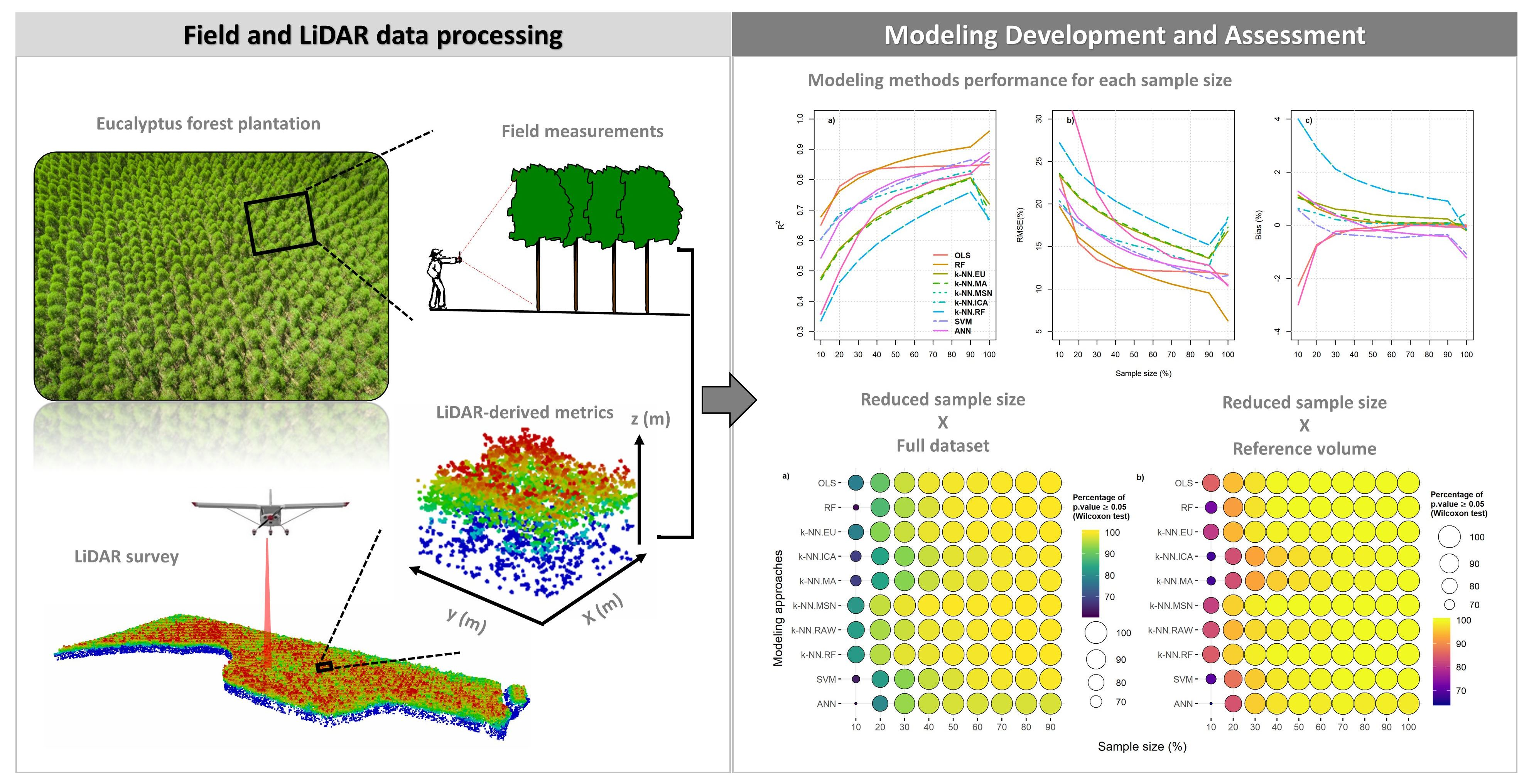
2. Materials and Methods

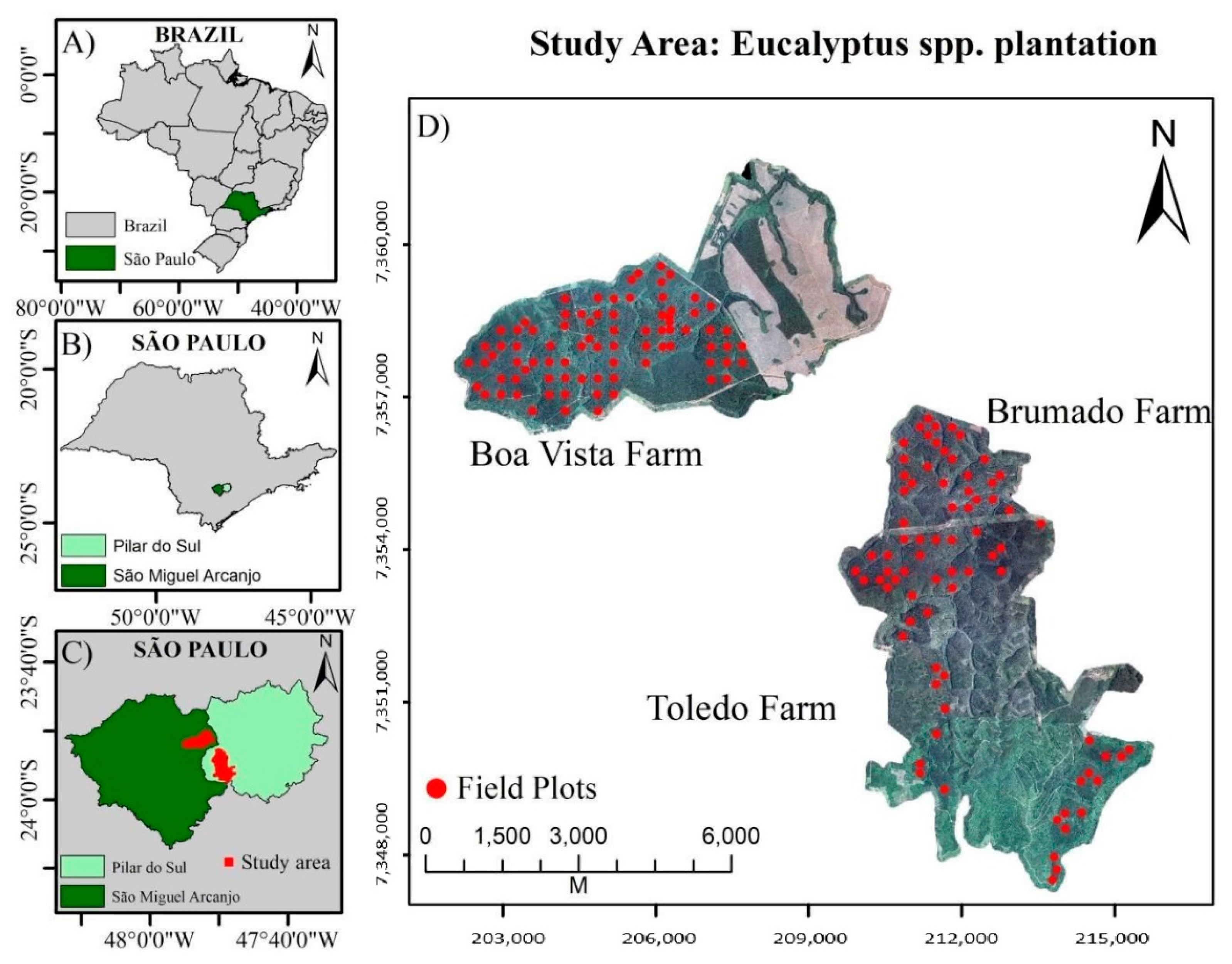
2.1. Study Area

The study area consisted of three farms located in the municipalities of Pilar do Sul and São Miguel Arcanjo, the southeast region of the state of São Paulo, Brazil (Figure 1). According to the Köppen classification, the climate of the region is characterized as humid subtropical, with wet and hot summers and dry and cold winters. The mean annual precipitation is ~1700 mm, and the mean annual temperature is 18.8 °C [32]. The topography in the selected plantations ranges from mildly hilly to very hilly, with an elevation ranging from 659 m to 1210 m. The soils of the region are predominantly red and yellow-red latosol, all classified as clayey or very clayey.

The farms contained industrial Eucalyptus plantations managed by Suzano S.A., a pulp and paper company located in São Paulo state, Brazil. The plantations were composed of hybrid clones of two Eucalyptus species, Eucalyptus grandis W. Hill ex Maid and Eucalyptus urophylla S.T. Blake, and covered an area of 2067.49 ha. All the trees were planted predominantly in a 3 × 2 m grid configuration, resulting in an average density of 1667 trees/ha. Standage across the farms was variable and ranged from 2 to 6 years.

2.2. Field Data

This study was based on data collected in a set of temporary and permanent sample plots installed for the purpose of annual forest inventory by the Suzano S.A. company. A total of 158 circular plots of 400 m² were established in stands ranging in age from 2.2 to 6 years. In each stand, the plot was randomly established within the stand boundary. Measurements were carried out during the months of April to November of 2013. All the sample plots were georeferenced in the field using a geodetic GPS (Global Positioning System) unit with differential correction capability (Trimble Pro-XR). The projected coordinate system used was UTM SIRGAS 2000, zone 23 S.

In each sample plot, individual trees were measured for diameter at breast height (dbh; cm) at 1.30 m, and a random subsample (15%) of trees for tree heights (Ht; m). Heights of unmeasured trees were estimated using locally adjusted hypsometric models, which use dbh as the predictor of Ht, following the model below:

$$ln\left(Ht\right)={\beta }_0+{\beta }_1\times \left(\frac{1}{dbh}\right)+\epsilon$$

(1)

where ln(Ht) = the natural logarithm of tree total height (m), β₀ and β₁ = the intercept and the slope of the model, dbh = diameter (cm) at breast height (1.30 m), and ε = model’s random error. Coefficients of determination (R²) and standard error (SE) were 0.97 and 3.18 m (6.09%).

Field measurements were used to estimate stem total volume (V; m³·tree⁻¹) by applying the respective diameter and height into the Schumacher–Hall allometric model [33], adjusted for each region, rotation, and genetic material, following the model below:

$$ln\left(V\right)={\beta }_0+{\beta }_{1}ln\left(dbh\right)+{\beta }_{2}ln\left(Ht\right)+\epsilon$$

(2)

where ln(V) = the natural logarithm of stem total volume (m³), β = model’s parameters to be estimated (i = 0, 1, 2), dbh = diameter (cm) at breast height (1.30 m), Ht = total height, and ε = model’s random error.

All the field measurements and predictions calculations from the hypsometric and allometric models were provided by the inventory team of Suzano S.A. The coefficients of the models are under the company’s intellectual property rights and not made available to the public; however, the R² and SE of the estimate for the volume models used in this study ranged from 0.96 to 0.98 and 8.3 to 12.7 m³·ha⁻¹ (3.18% and 6.09%), respectively. Each variable of all individuals was summed at plot-level and scaled to a hectare. A summary of plot-level forest attributes, including V (m³·ha⁻¹) calculations for each class of stand ages, is presented in

Table 1. Summary statistics of forest attributes from ground measurement at the sample plots.

Ages	dbh (cm)		Ht (m)		V (m3·ha−1)		N Plots
	Mean	SD	Mean	SD	Mean	SD
2.2	10.27	1.19	14.34	1.23	58.34	20.30	6
3.2	12.75	0.88	21.83	1.05	160.35	24.77	5
3.8	14.09	0.56	22.35	1.49	189.15	23.87	10
4.5	15.55	1.32	25.90	0.86	280.63	39.35	5
4.8	15.82	0.87	29.34	1.38	329.44	42.14	37
5.1	15.36	1.06	28.62	1.67	333.35	55.23	38
6	16.51	1.56	29.13	2.81	349.53	87.25	57

SD: standard deviation, dbh: diameter at breast height, Ht: total height.

.

2.3. LiDAR Data Collection Specifications and Processing

An airborne LiDAR survey was conducted in the study area on 5 December 2013, using a Harrier 68i sensor (Trimble, Sunnyvale, CA, USA) mounted on a CESSNA 206 aircraft. The characteristics of the LiDAR data acquisition are listed in

Table 2. Airborne Light Detection and Ranging (LiDAR) survey specifications.

Parameter	Value
Scan angle (°)	±45°
Footprint	0.33 m
Flying altitude	438 m
Swath width	363.11 m
Overlap	100% (50% side-lap)
Scan frequency	300 kHz
Average point density	10 pts·m−2

. LiDAR data processing steps were performed using FUSION/LDV 3.7 software [34], which provided three major outputs: the digital terrain model (DTM), the normalized point cloud, and the LiDAR-derived canopy structure metrics.

In order to differentiate between ground and vegetation points, the original LiDAR cloud data were filtered using the classification algorithm proposed in Reference [35]. The ground points were used to generate the 1 m resolution Digital Terrain Models (DTMs). The LiDAR clouds were normalized to heights by subtracting the DTMs elevations from each LiDAR return. Normalized point clouds were subset within the field sample plots of interest, and the canopy metrics were computed at plot using all returns above 1.30 m. We generated only those metrics that have been often used as candidate predictors for forest attribute modeling in other recent studies [14,20,36,37]. Therefore, a total of 26 LiDAR metrics calculated from all returns were considered as a candidate for predicting stem volume (

Table 3. LiDAR-derived structure metrics considered as candidate predictor variables.

Variable	Description	Variable	Description
HMAX	Height maximum	H25TH	Height 25th percentile
HMEAN	Height mean	H30TH	Height 30th percentile
HMODE	Height mode	H40TH	Height 40th percentile
HSD	Height standard deviation	H50TH	Height 50th percentile
HVAR	Height variance	H60TH	Height 60th percentile
HCV	Height coefficient of variation	H70TH	Height 70th percentile
HIQ	Height interquartile distance	H75TH	Height 75th percentile
HSKEW	Height skewness	H80TH	Height 80th percentile
HKURT	Height kurtosis	H90TH	Height 90th percentile
H01TH	Height 20th percentile	H95TH	Height 95th percentile
H05TH	Height 20th percentile	H99TH	Height 99th percentile
H10TH	Height 20th percentile	CR	Canopy relief ratio $\frac{HMEAN-HMIN}{HMAX-HMIN}$
H20TH	Height 20th percentile	COV	Canopy cover (percentage of first returns above 1.30 m)

). All the LiDAR processing was performed by FUSION/LDV [34].

2.4. Modeling Development and Assessment

The modeling approaches evaluated in this study to estimate the statistical relationship between stem volume and LiDAR metrics fall into two different categories: parametric methods (e.g., multiple linear regression) and non-parametric methods (e.g., machine learning regression). Parametric and non-parametric models have been proven to be useful for developing predictions from LiDAR-derived metrics and field-estimated forest structural attributes [20,31,36,37,38,39]

Even though machine learning algorithms are usually not sensible for collinearity, normality, or linearity, in order to obtain a set of predictor variables that could be commonly applied to all the selected modeling methods, we used two variable selection approaches. First, Pearson’s correlation (r) analysis was carried out to identify highly correlated metrics and to exclude redundant predictors (r > 0.9) [31,40]. Second, we implemented principal component analysis (PCA) to the most relevant LiDAR-derived candidate metrics to achieve a final set of predictor variables. Using PCA, a subset of variables that explain the majority of variation can be selected from a large set of (possibly highly correlated) predictor variables.

PCA was applied over the selected LiDAR metrics for each of the 158 sample plots. A correlation matrix derived from the LiDAR metrics provided the basis for the eigenvalue and eigenvector calculations and for the subsequent determination of the PC scores. Each score represented a transformed metric from the linear combination of the LiDAR metrics of the sample plots. By analyzing the eigenvectors and the PC score, we established differences in the contribution of each LiDAR metric to the variability in the dataset, as well as the similarity in metrics calculated across the different aged stands [14]. The first five metrics that were most likely to contribute to the model development were identified by inspecting the eigenvectors in each PC. We then used the metrics with the highest loading on the PCs as input variables for every modeling method.

For assessing the effect of modeling approaches for predicting stem total volume in Eucalyptus forest plantation, we used the following modeling approaches:

(i)

Ordinary least-squares (OLS) multiple regression: The OLS regression algorithm fits a linear model by minimizing the residual sum of squares between the observed values in the training dataset and the predicted values by the linear model [41].

(ii)

Random forest (RF) algorithm: RF is a combination of a decision tree with a value of a random independently sampled vector and with the same distribution for all trees in the forest [22]. Based on binary rule-based decisions, the algorithm indicates which particular tree should be used for each specific data input. RF was adjusted using 1000 trees, and one-third of the number of variables to be randomly sampled at each split.

(iii)

k-nearest neighbors (k-NN) imputation: k-NN methods work by direct substitution (imputation) of measured values from sample locations (references) for locations for which we desire a prediction (targets). In this strategy, key considerations include the distance metric that is used to identify suitable references and the number of references (k) that are used in a single imputation [20]. In this study, we examined k = 1 neighbors for each of the mentioned distance metrics in order to keep the original variation in the data [42]. Many imputation methods can be used for associating target and reference observations. We decided to evaluate six different distance metrics for the k-NN-based approach: raw, Euclidean (k-NN-EUC), Mahalanobis (k-NN-MA), most similar neighbor (k-NN-MSN), independent component analysis (k-NN-ICA), and random forest (k-NN-RF).

(iv)

Support vector machine (SVM): SVM considers a statistical learning principle to fit a hyperplane that superimposes as much training data as possible. Instead of error minimization, SVM uses structural risk minimization of the distance from training points to the hyperplane [43,44]. To warranty a nonlinear response space, our SVM uses a Radial Base Function for the Kernel function.

(v)

Artificial neural network (ANN): The ANNs algorithm is inspired by the work of neurons in the human brain [45]. The neural network was set up with two hidden layers: 7 neurons in the first layer (same length of the variables vector) and one neuron in the second layer. The initial weights were set randomly, and the decay parameter was set to 0.1.

For assessing the effect of the sample size within each modeling approach, the models were embedded in a bootstrapping approach with 500 iterations. In each bootstrap iteration, we drew from 10% to 90% the number of observations with replacement from the available samples and validated the model with all observations. In each bootstrap iteration, relative root mean square error (RMSE; Equation (3)), coefficient of determination (R²; Equation (4)), and bias (Equation (5)) were computed based on the linear relationship between observed and predicted volumes.

$$RMSE=\sqrt{\frac{{\sum }_{i=1}^n{\left(y_i-{\widehat{y}}_i\right)}^2}{n}}$$

(3)

$$R^2=1-\frac{{\sum }_{i=1}^n{\left(yi-\widehat{y}i\right)}^2}{{\sum }_{i=1}^n{\left(y_i-\underset{\_}{y}\right)}^2}$$

(4)

$$Bias=\frac{1}{n}{\displaystyle \sum }_{i=1}^n\left(y_i-{\widehat{y}}_i\right)$$

(5)

where y_i is the observed value for plot i, ŷ_i is the estimated value for plot i, and n is the number of plots. Relative RMSE and bias were calculated by dividing the absolute values by the mean of the observed response parameters. We defined acceptable model precision and accuracy as a relative RMSE and bias of ≤15% to have a model precision and accuracy higher than or equal to the conventional forest inventory standard in fast-growing Eucalyptus plantations in Brazil [31].

2.5. Statistical Comparisons

Considering each tested modeling approach, to assess how the combined effect with sample size may impact the accuracy of the predictions, we used the Wilcoxon–Mann–Whitney test to determine if the differences between the methods and sample sizes were statistically significant (at p-value = 0.05). We developed all the statistical analyses in the R statistical package [46]. The RF algorithm was implemented by package randomForest [47], k-NN by yaImpute package [48], in combination with the randomForest package [47], the SVM by the e1071 package [49], and the ANN was implemented by the nnet package [50].

3. Results

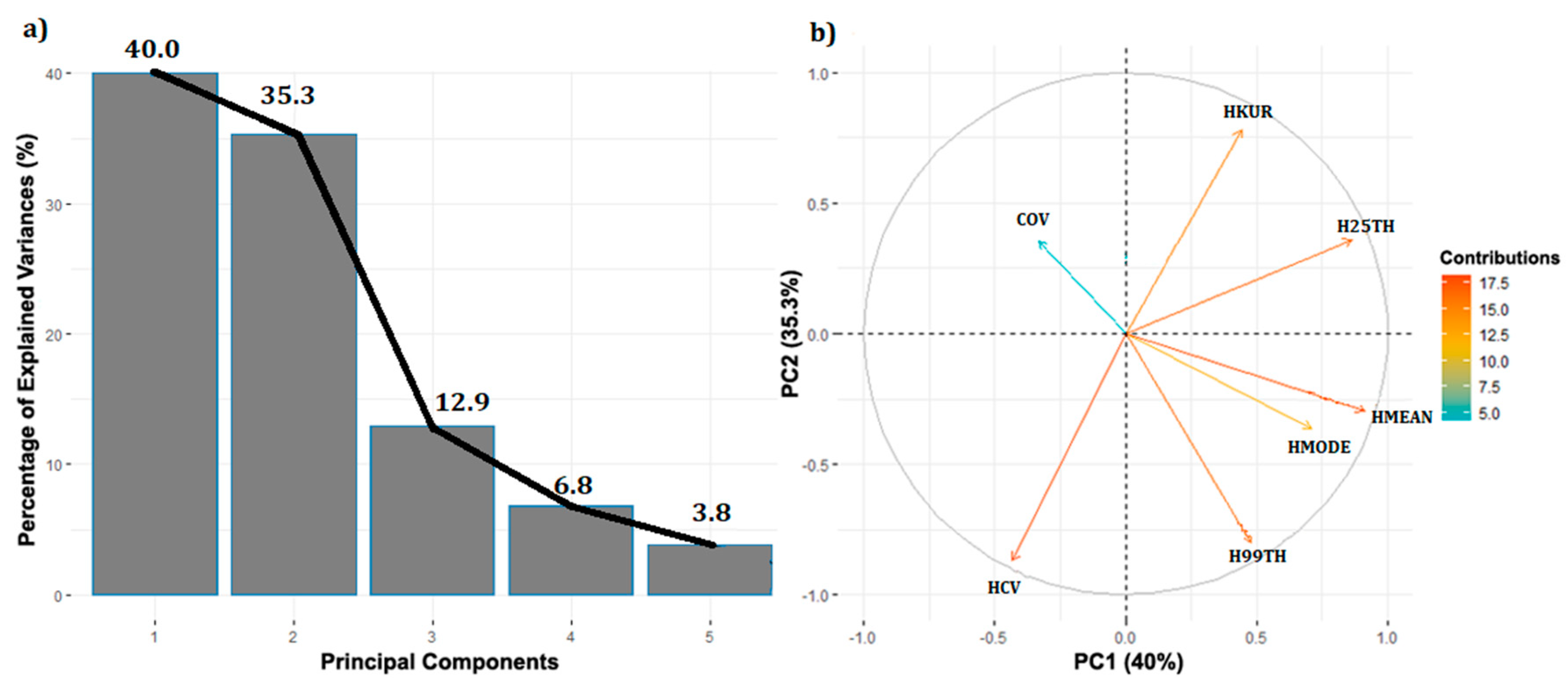
3.1. Predictor Variable Selection

A total of 19 of the 26 LiDAR metrics showed a very strong correlation (r > 0.9). To represent the 19 metrics, we retained the H99TH along with six other remaining metrics not highly correlated (r ≤ 0.9) (

Table 4. Pearson correlations among selected LiDAR metrics.

r	HMEAN	HMODE	HCV	HKUR	H25TH	H99TH	COV
HMODE	0.66 ***
HCV	−0.10	−0.02
HKUR	0.23	0	−0.79 ***
H25TH	0.67 ***	0.39 **	−0.69 ***	0.54 ***
H99TH	0.76 ***	0.52 ***	0.53 ***	−0.32 *	0.10
COV	−0.27	−0.24	−0.07	0.22	−0.23	−0.26

***: p-value < 0.001; **: p-value < 0.01; *: p-value < 0.05; If there is no *: p-value ≥ 0.05.

). HMEAN, HMODE, HCV, HKUR, H25TH, H99TH, and COV were included in the PCA. Among these, HMEAN, HMODE, HKUR, H99TH, and COV exhibited the highest PC eigenvector loadings (

Table 5. Loadings and eigenvectors for the first five principal components (PCs).

PCs	Ev	Eigenvectors (Eg)
		HMEAN	HMODE	HCV	HKUR	H25TH	H99TH	COV
PC1	2.80	0.54	0.42	−0.26	0.26	0.52	0.29	−0.20
PC2	2.47	−0.19	−0.23	−0.55	0.50	0.23	−0.51	0.23
PC3	0.91	0.19	0.14	0.14	0.19	−0.13	0.25	0.90
PC4	0.48	−0.29	0.84	−0.13	−0.21	−0.12	−0.36	0.08
PC5	0.27	0.01	−0.17	−0.14	−0.71	0.58	−0.07	0.31

PC is the given principal component; Ev is the eigenvalue for each PC. Bold values indicate the largest contributing LiDAR metric for a given PC.

), which represented the contribution of each LiDAR metric toward the component, and therefore, were used for model development.

The first five PCs accounted for 98.9% of the total variance contained in the selected set of seven LiDAR metrics. PC1, PC2, PC3, PC4, and PC5 accounted for 40.0%, 35.3%, 12.9%, 6.8%, and 3.8% of the total variance, respectively (Figure 2a). PCs 6–7 explained a less than significant percentage (<2.5%) of the remaining variance and were discarded. The first PC captured the canopy height variation and showed positive loadings by height metrics (i.e., HMEAN and H25TH) and negative loading of metrics of HCV and COV. The second PC was mainly influenced by density metrics, and the third PC highlighted canopy cover.

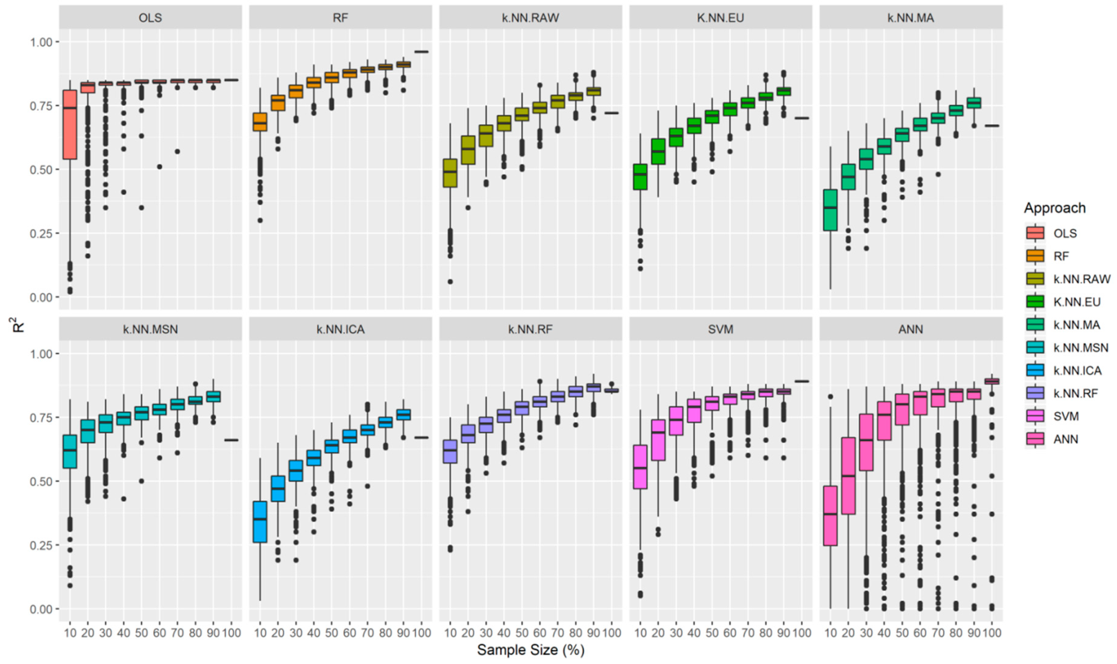
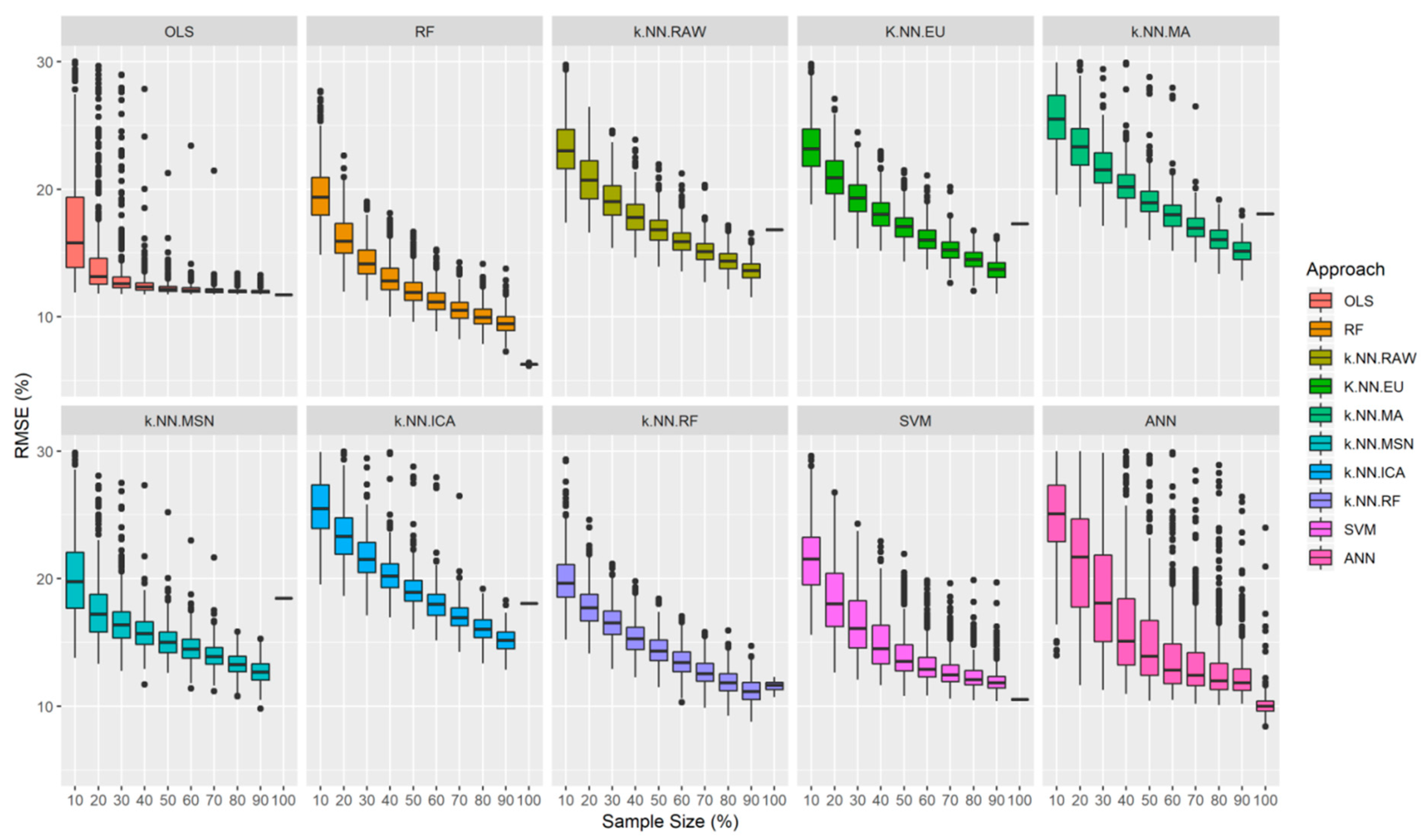
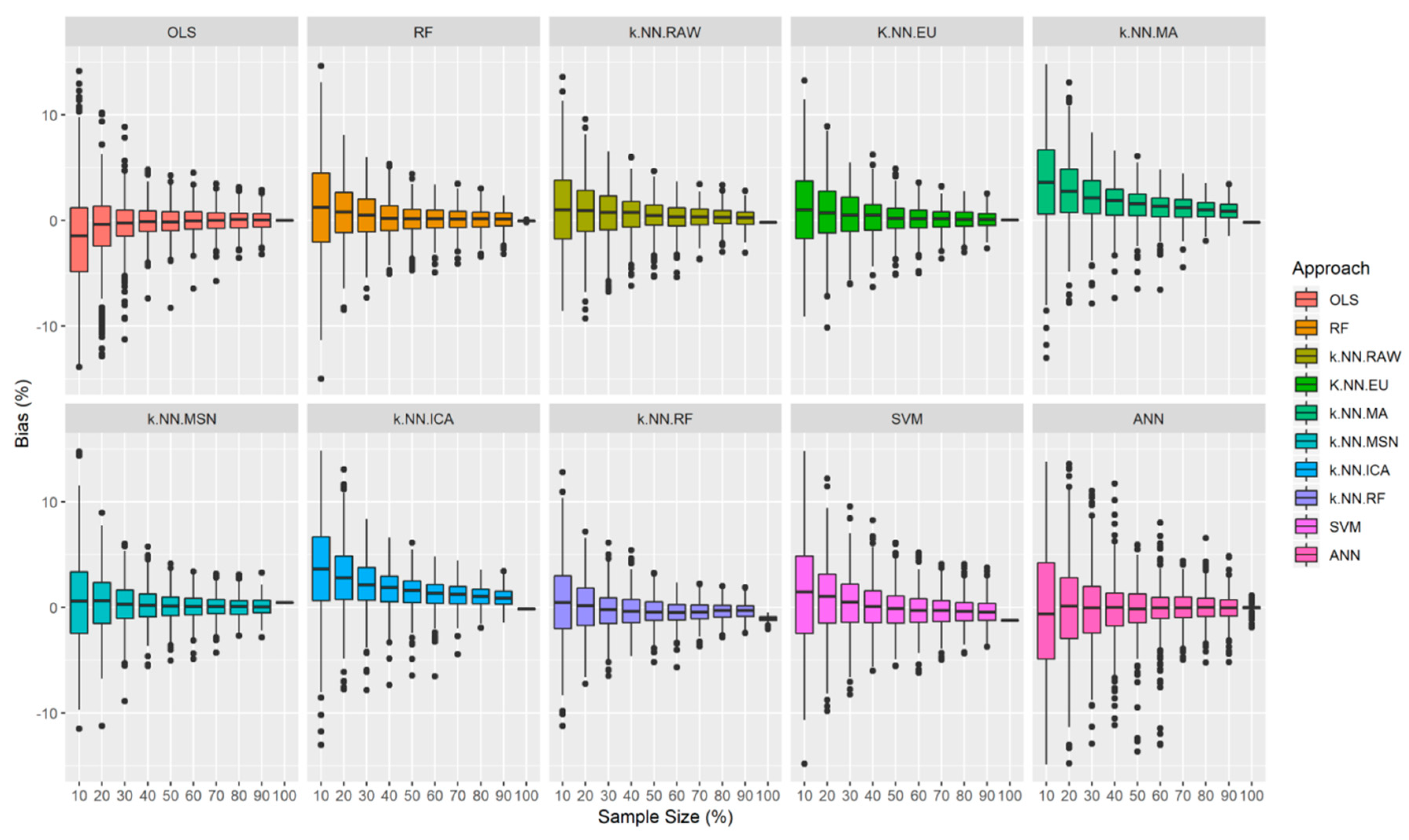
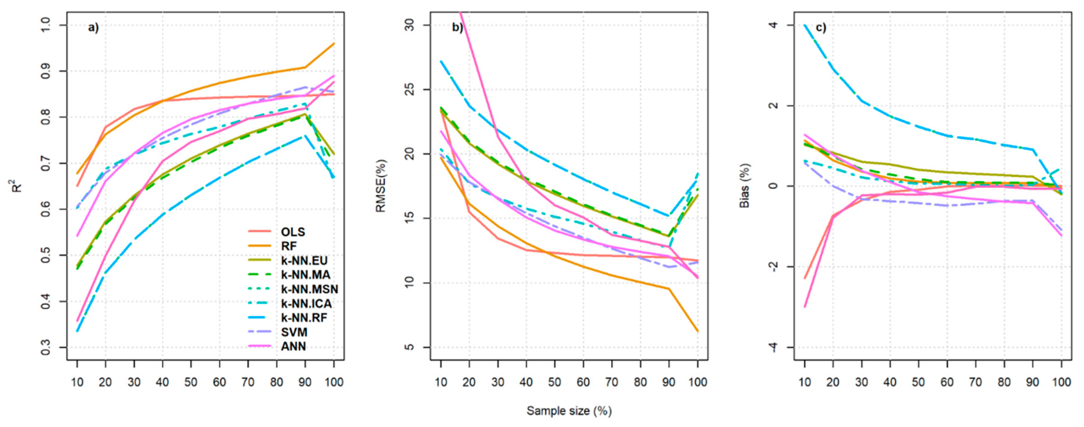
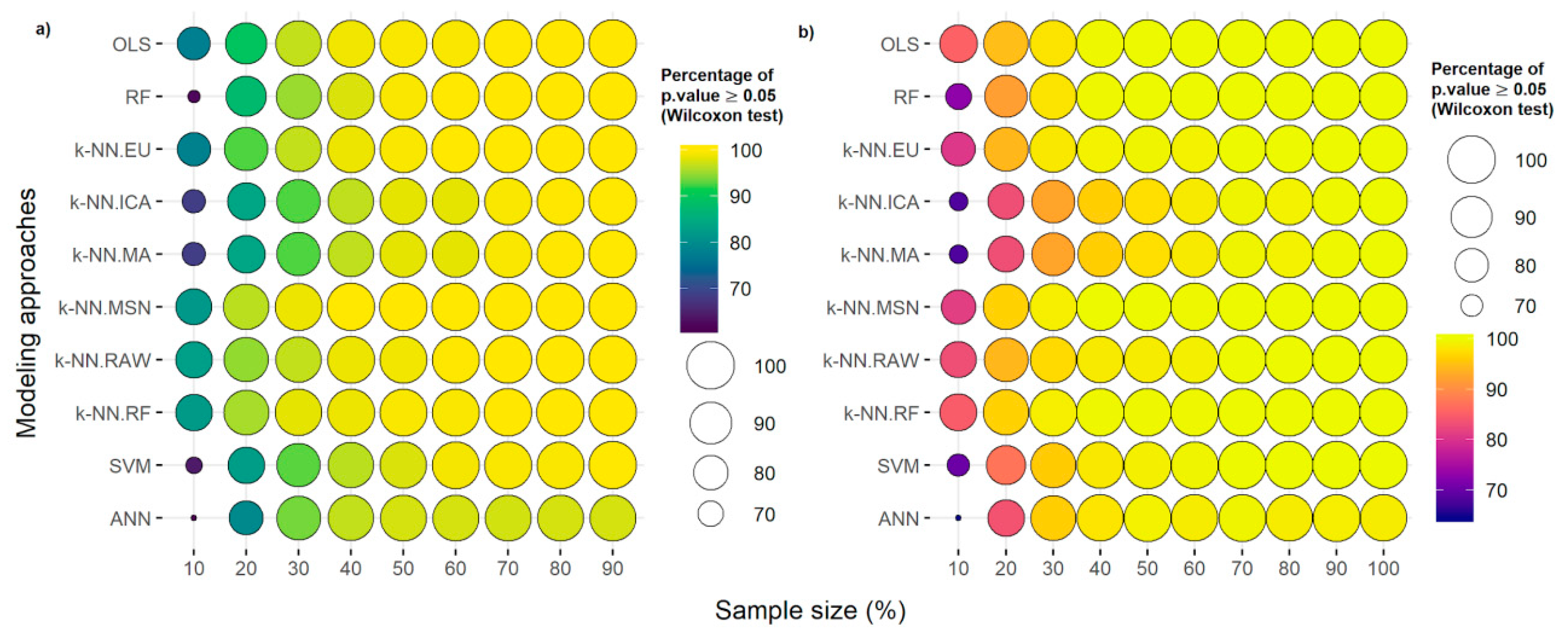
3.2. Combined Impact of Sample Size and Data Modeling

The evaluation of the modeling methods’ accuracy throughout the sample size was carried out by three performance measures indicators: R², RMSE, and bias (Figure 3, Figure 4 and Figure 5). Comparisons across the ten prediction methods indicated that OLS and RF outperformed the other tested methods. A relatively stable increase in accuracy and decrease in RMSE were observed along with increasing sample size in all methods, but only the OLS and RF methods were able to meet the acceptable model precision criteria (RMSE and bias of ≤15%) from 30% of the sample size. OLS presented R² values ranging from 0.82–0.85 for 30% to 90% of the sample size and demonstrated a more stabilized pattern. In terms of Bias, the variation with respect to increased sample size was very balanced, which shows the robustness of the model. The RF method showed more sensitivity towards the number of samples and presented R² values in the range of 0.80–0.91 for 30% to 90% of the sample size. When the sample size was over 50%, the R² values of the RF algorithm were higher than that compared to the OLS models.

The SVM algorithm presented similar performance to the RF algorithm, however showing lower values in all parameters evaluated. The algorithm was able to meet the acceptable model precision criteria (RMSE and bias of ≤15%) from 50% of the sample size, presenting R² values ranging from 0.80–0.85 for 50% to 90% of the sample size. From the six derivations of the k-NN algorithm tested, the RF-based k-NN approach showed the best results and was able to meet the criteria while using 50% of the sample size, presenting R² values ranging from 0.78–0.86 for 50% to 90%. The poorest performance in this k-NN group was found to be for the k-NN MA algorithm, which presented a relative RMSE of 18.06%, a bias of −0.18%%, and R² of 0.67, even when the sample size was 100%. The k-NN ICA algorithm also behaved in a similar fashion. Among all the machine learning algorithms, ANN presented the worst performance in terms of outliers.

The best method and sample size combination (minimum sample size) to provide better R² values and a relatively lower number of outliers was found to be OLS with 40% of the sample size (which accounts for a sample size of n = 63 and ~0.04 plots/ha). The use of only 40% of the full dataset combined with the OLS method was able to provide an average of 0.83 for R² and 12.53% and −0.14% for relative RMSE and bias, respectively. No significant improvement for predicting stem volume was found by increasing the sample size from 40% to 50%. The Wilcoxon test comparing RMSE values derived from 40% with the full (100%) dataset showed a p-value > 0.05; hence, 40% and 100% had similar distributions and mean, evidencing no significant difference between them. Whereas, in the case of RF, at a 40% sample size, we obtained an average of 0.78 for R² and 13.07% and 0.19% for relative RMSE and bias, respectively.

Furthermore, we created two generic visual representations to help us distinctly comprehend and compare performance trends of various modeling techniques—in terms of R², RMSE%, and relative bias (Figure 6), in addition to volume predictions derived from reduced sample sizes (Figure 7). For instance, it is easy to notice from Figure 6a how R² of OLS keeps increasing with sample size, how this compares with respect to RF, and at what point their performances are overlapping—in this case at around 20% and 40% sample sizes—and switching of trends which denotes higher sensitivity of RF towards sample sizes. The same applies to other modeling techniques as well as the RMSE%- and bias-related line graphs presented in Figure 6 (b and c, respectively). In Figure 7, we present the percentage of times we obtained a p-value > 0.05 for the Wilcoxon test (from a sum total of 500 iterations) for a particular combination of sample size and modeling approach with respect to the full dataset (Figure 7a) and reference volume (Figure 7b). Herein, if we look at the Figure 7a, we notice that when volume predictions from various combinations of sample size levels (10% to 90%) are compared to the full LiDAR-based dataset, for most of the modeling approaches, adding more than 40% of the sample size does not make any accountable difference—that is, for example, if we take the case of OLS, the high percentage of p-value > 0.05 for 40% of data represents that this amount of sample size gives mean and spatial distribution similar to using 100% of data; on the other hand, in the case of ANN, even at 90% sample size, the percentage of p-value > 0.05 does not reach 100%, denoting its inapplicability. However, these results do not represent precise predictions or might not provide high accuracy as they are based on 500 iterations where sample points are taken randomly and evaluated for calculating p-values and total percentage. Hence, each time we run the model, our observations can be different, and we cannot be sure that the one we obtained at a particular time exactly represents the real scenario. Nonetheless, we can notice how much sample size % in average is needed with respect to a parametric or non-parametric algorithm to reach 100% in terms of p-values, and this allows us to evaluate the stability of models across sample sizes. Whereas, in Figure 7b, we observe a much smoother trend—that is, above 30% sample size, most of the modeling approaches give 100% in p-values > 0.05. This is because the respective model-based predicted volumes are being compared with reference (inventory-based) volumes which are fixed values.

4. Discussion

Although LiDAR has shown to be a powerful technology for forest inventory around the world, its application for monitoring Eucalyptus forest plantations in Brazil is relatively new [18,51]. On examination of the trends observed in previous studies, that have employed a wide range of modeling methods for forest attribute estimation and reported results representing varying accuracies, it is clear that appropriate selection of methods is paramount for attaining the best prediction results [20,37,44,52,53]. The novelty of this research is to investigate how the combined influence of sample size and different modeling techniques affect the overall prediction accuracy of forest plantation attributes and demonstrate the potential of reduced sample sizes to generate accurate prediction results.

For reducing model complexity and boosting overall prediction accuracy, it is imperative to select a minimal number of parameters by means of variable selection approaches [14,54]; this task, however, gets more challenging when highly correlated predictors are present. Application of dual variable selection approaches—Pearson’s correlation analysis and PCA—proved beneficial in our case and allowed us to shortlist the five major variables: HMEAN, HCV, HMODE, HKUR, and COV, from a total of 26 LiDAR metrics. These five variables, which were used for model development, accounted for 98.9% of the total variation contained in the pre-selected set of LiDAR metrics. Recent studies done on Eucalyptus plantations which had applied PCA for variable selection, found similar total variance contained in the selected set of LiDAR metrics (97.7%) and showed HCV, H99TH, COV, H01TH, and H05TH as the most important variables for predicting stem volume [14].

There was a significant relationship between field-based volume estimates and LiDAR-derived metrics selected from the PCA analysis. The selected metrics from the PCA analysis were consistent with previous studies which have also observed that mean height had the largest absolute correlation with the first principal component, coefficient variation of height had the largest absolute correlation with the second principal component, and canopy cover had the largest absolute correlation with the third principal component [55]. Models using these three first principal components likely capture the fundamental allometric relationships between volumes and heights, as seen in results from large-footprint data [15], in which mean height, canopy cover, and height variability were found to explain most of the variability in forest physical characteristics. Several previous studies [56,57] have also found that metrics such as HMEAN and HCV have shown to be effective predictors of forest attributes, such as stem volume, height, basal area, and aboveground carbon in Eucalyptus spp. plantations. The biological basis behind these results is due to the ecological and biomechanical links between canopy vertical structure and forest stand structure parameters. From the perspective of tree form and function development, there is usually a connection between the differences in vertical canopy structure and differences in forest volume, both through forest succession and across areas with contrasting environmental conditions [55].

From our results, it was evident that algorithm performance was sensitive to sampling size and the level of influence varied from one algorithm to another. On placing constraints (<15%) for RMSE values, only 4 models—SVM, RF-based k-NN, RF, and OLS—were found to be feasible for making predictions for 50% (or less) of the sample size. In the case of OLS and RF, a sample size greater than 30% fell within the RMSE threshold. For OLS, this might be because of the low level of multicollinearity within the model. Whereas, for RF-based k-NN and SVM, the ideal sample sizes were equal to or above 50%. In terms of bias, we noticed that all the models fell within the maximum set limit, which was 15%. With respect to R² values, OLS proved to be the best among the given modeling methods, followed by RF, when minimal sample size was given priority. The range of R² values was comparatively stable for OLS: 0.82–0.85 for 30% to 90%; however, RF: 0.80–0.91 for 30% to 90%, reached higher values when the sample size was increased. The increase in R² values with increasing sample size was very evident in the case of other non-parametric models as well. However, this pattern was expected, considering the fact that the non-parametric models learn their functional form from the training data [52,58], which means that the higher the sample size, the better their prediction accuracy will be. This dependence on sample size might be the reason several other non-parametric algorithms failed to provide satisfactory results in our case, where field plots considered were limited [20,59].

Even though for OLS, sample size above 30% met the chosen criteria, high levels of outliers were observed in this case. A former study [60] came up with the generalization that average standard deviation tends to increase with a reduction of sample size, which matches our findings very well. However, the sample size on reaching 40% showed a significant reduction in the number of outliers. On further increase to 50% of the sample size, not much difference occurred in the outliers count or the R² values. Additionally, by performing the Wilcoxon test (p > 0.05), we confirmed that 40% and 100% were not significantly different in terms of distribution and mean. When the sample size was 30%, RF also gave satisfactory results, even though the R² value was slightly lower (0.8) compared to OLS (0.82). Based on our results and core objective—which was to find the minimum sample size required for attribute estimation—we inferred the best combination to be the linear regression (OLS) model with a sample size of 40%, followed by the random forests (RF) method with an identical sample size value.

Since there existed no extensive studies that accounted for the combined influence of modeling methods and sample size, evaluating the accuracy of our model in regard to established and identical workflows was near impossible. Nevertheless, in comparison with studies that have evaluated the influence of sample size and modeling methods on a discrete basis, we noticed our obtained trends and accuracy of the high performing models to be quite comparable with the inferences made by other studies. A recent study [61] investigated the influence of number and size of sample plots, as well the effect of a single selection, on modeling growing stock volume (GSV) of a Scots pine (Pinus sylvestris L.)-dominated forest in Poland, with 900 available study plots, using airborne LiDAR data. Based on their three major findings: (i) influence of number of sample plots on the accuracy of GSV estimation above 400 sample plots was nominal, (ii) number of sample plot size and estimation accuracy revealed an inverse relationship, irrespective of the number of plots considered, and (iii) single selection does not have any impact when plots considered were above 400, the authors concluded that it is possible to reduce the number of ground sample plots by almost one-third and still retain reasonable accuracy and precision levels, even when the sample plot area is relatively small. This was highly evident in our case as well—for a sample size of less than 40%. Caution is necessary to evaluate the accuracy per age (or another sub-population), since we have unbalanced number of samples per group (Table 1). We did not explore in this study the sample size for groups within the population.

Another study [20] compared the performance of seven modeling methods—k-NN-MSN, gradient nearest neighbor imputation, k-NN-RF, Best NN imputation, OLS, spatial linear model, and geographically weighted regression—for predicting five forest attributes, including basal area, stem volume, Lorey’s height, quadratic mean diameter, and tree density, from airborne LiDAR metrics in a mixed conifer forest in southwestern Oregon, in the United States. Contrary to our results, in this case, the authors were not able to come up with a single modeling method that always performed superior to the others in the prediction of the forest attributes; nonetheless, OLS and the spatial linear model gave the best results in terms of RMSE values in the maximum number of cases. From the paragraphs above, we can see that OLS has consistently returned similar estimates (and performance) as compared to more advanced methods, being consistently included among the best models. OLS also has an important advantage when considering the facility to find out the explanatory power of independent variables and make comparison to models generated by other studies.

The major takeaway from our study is that with LiDAR data of only 40% of the total field plots, we are able to make accurate predictions, given that the right modeling technique is employed. This, when translated into large-scale area projects, means savings of a huge amount of money and faster processing with high accuracy. With the same amount of time, we can get more things done or maybe even utilize the available budgets for performing surveys at an increased frequency. Future studies can even narrow these results by reducing the intervals in sample size (that is, instead of the 10% used here, perhaps use 5% or even 1%) and repeating the same process.

Results also highlight that multiple modeling methods work well on predictions and depending on the level of data in hand, these methods can be selected. However, it is incumbent on the modelers to keep in mind the limitations of each algorithm before applying them. For example, for applying linear regression models, assumptions of a linear relationship, homoscedasticity, etc., need to be met, and this is not always true in the case of several plantation data. In a lot of cases, since the data is collected from a copious amount of sources and often has data of the same location for multiple dates, a data hierarchy tends to exist, and in this case, a mixed-effects model needs to be used to account for the random effects happening within the models [62,63,64,65,66]. Therefore, a minimum knowledge of the study site and exhaustive data exploratory analysis is recommended before making the method selection. One should also acknowledge the errors associated with field measurements, ALS data acquisition, and data processing steps while interpreting the model results.

Previous studies have reported the minimum sample size required to vary with respect to the attribute and tree species under consideration. For instance, a study undertaken by the authors of Reference [67] observed the accuracy of estimated Picea abies (L.) Karst volumes at the forest stand level to show no decrease until the number of plots was reduced to below 200 (46.4% of the total number of sample plots). Whereas, for the case of other deciduous tree species, the volume estimation accuracy plummeted, with a gradual decrease in the number of sample plots. Also, more often than not, limited field data and/or acquired LiDAR data quality place additional constraints on complementing studies that intend to evaluate the minimum sample size required for estimating the accuracy of forest attributes using LiDAR metrics [61].

Here, we tested the combined influence of only sample size and modeling algorithms, nonetheless, the influence of additional features, such as plot size, LiDAR pulse density, GPS location errors, etc., would also be interesting and helpful to the research community [52,68,69]. Another thing to keep in mind is the cost associated with LiDAR, which makes this approach economically feasible for only large study areas [10,31,70]. It is always a possibility to improve estimation by adopting a proper sampling method. A combination of field data and LiDAR considering a double sampling approach can significantly reduce the estimation error [71].

Updating data over time using LiDAR can be perceived as a hurdle for the same reason. However, if we are willing to adopt a different perspective, that views the potential reduction of fieldwork cost as compensation for ALS data acquisition, then multiplying the ALS data collection frequency can be treated as a reasonable initiative. Data fusion techniques that integrate LiDAR with other more affordable methods such as unmanned aerial vehicle (UAV) remote sensing or other low-cost, available cutting-edge technologies, can be deemed as an interesting strategy having great potential for forest plantation assessment [11,72,73,74,75].

Translating this framework from the research to the operational arena requires additional work, especially to test its applicability on multiple sites and to verify stability in results, which needs more investment in terms of fieldwork and analysis. Even so, the expected benefits, that come in the form of reduced inventory cost in the forest plantation sector, will be a huge leap for the forest management sector.

5. Conclusions

The importance of a framework with more robust and accurate techniques that consider auxiliary data in the process of estimating stem total volume is evident. In this study, we evaluated the impacts of different modeling methods and sample size on the accuracy of volume estimates predicted from LiDAR data in a Eucalyptus forest plantation in Brazil. Our results showed that the precision of LiDAR-derived stem total volume estimates was considerably impacted by the prediction method while varying sample sizes. Higher levels of accuracy were obtained by employing a multiple linear regression model, which was able to provide comparable results using only 40% of the total field plots (~0.04 plots/ha), followed by the random forest with an identical sample size value. The precision of the combined impact of sample size and modeling methods was demonstrated through a relative RMSE and bias less than 15%, which is equal to or less than the level of error that is traditionally accepted in a conventional field inventory. The methods used in this study formulate a framework for integrating field and LiDAR data, highlighting the importance of sample size for volume estimates.

The major takeaway from our study indicates that collecting larger field reference data is not necessarily the most effective option for improving the accuracy of volume estimates while dealing with forest plantations, which in general comprise of relatively simple vegetation structures. Thus, this study should be able to assist in the selection of an optimal sample size that minimizes estimation errors, processing time, and plot establishment costs. Future directions for this research include the use of a larger number of datasets that tests additional features (i.e., plot size, LiDAR pulse density, GPS location errors), integrating multi-sensor data fusion approaches (i.e., terrestrial or UAV LiDAR, radar), and estimating forest attributes at an individual tree level. Additionally, the development of further studies to increase our understanding of the statistical modeling methods’ role in the volume estimation of this forest type would be able to shed more light on the ideas presented herein. We hope that the findings from our study give more credibility and encouragement for specialists to pursue research in directions that will ultimately result in the development of site-independent LiDAR data-based models for predicting a wide range of forest attributes.

References

1. FAO (Food and Agriculture Organization of the United Nations). Global Forest Resources Assessment 2015: How Are the World’s Forests Changing? FAO: Rome, Itally, 2015; p. 9. Available online: http://www.fao.org/3/a-i4793e.pdf (accessed on 21 August 2019).
2. Gao, T.; Zhu, J.; Deng, S.; Zheng, X.; Zhang, J.; Shang, G.; Huang, L. Timber production assessment of a plantation forest: An integrated framework with field-based inventory, multi-source remote sensing data and forest management history. Int. J. Appl. Earth Obs. Geoinf. 2016, 52, 155–165. [Google Scholar] [CrossRef]
3. Rockwood, D.L.; Rudie, A.W.; Ralph, S.A.; Zhu, J.Y.; Winandy, J.E. Energy product options for Eucalyptus species grown as short rotation woody crops. Int. J. Mol. Sci. 2008, 9, 1361–1378. [Google Scholar] [CrossRef] [PubMed]
4. Indústria Brasileira de Árvores. Relatório Lbá 2019; Indústria Brasileira de Árvores: Brasília, Brazil, 2019; p. 80. Available online: https://iba.org/datafiles/publicacoes/relatorios/iba-relatorioanual2019.pdf (accessed on 21 August 2019).
5. Mohan, M.; de Mendonça, B.A.F.; Silva, C.A.; Klauberg, C.; de Saboya Ribeiro, A.S.; de Araújo, E.J.G.; Monte, M.A.; Cardil, A. Optimizing individual tree detection accuracy and measuring forest uniformity in coconut (Cocos nucifera L.) plantations using airborne laser scanning. Ecol. Model. 2019, 409, 108736. [Google Scholar] [CrossRef]
6. González-garcía, M.; Hevia, A.; Majada, J.; Anta, R.C.; Barrio-Anta, M. Dynamic growth and yield model including environmental factors for Eucalyptus nitens (Deane & Maiden) Maiden short rotation woody crops in Northwest Spain. New For. 2015, 46, 387–407. [Google Scholar] [CrossRef]
7. Retslaff, F.A.; Filho, A.F.; Dias, A.N.; Bernett, L.G.; Figura, M.C. Curvas de sítio e relações hipsométricas para Eucalyptus grandis na região dos Campos Gerais, Paraná. Cerne 2015, 21, 219–225. [Google Scholar] [CrossRef] [Green Version]
8. Morgenroth, J.; Visser, R. Uptake and barriers to the use of geospatial technologies in forest management. N. Z. J. For. Sci. 2013, 43, 1–16. [Google Scholar] [CrossRef] [Green Version]
9. Montaghi, A.; Corona, P.; Dalponte, M.; Gianelle, D.; Chirici, G.; Olsson, H. Airborne laser scanning of forest resources: An overview of research in Italy as a commentary case study. Int. J. Appl. Earth Obs. Geoinf. 2013, 23, 288–300. [Google Scholar] [CrossRef] [Green Version]
10. Silva, C.A.; Valbuena, R.; Pinagé, E.R.; Mohan, M.; de Almeida, D.R.; North Broadbent, E.; Wan Mohd Jaafa, W.S.; de Almeida Papa, D.; Cardil, A.; Klauberg, C. ForestGapR: An r Package for forest gap analysis from canopy height models. Methods Ecol. Evol. 2019, 10, 1347–1356. [Google Scholar] [CrossRef] [Green Version]
11. Dalla Corte, A.P.; Rex, F.E.; Almeida, D.R.A.D.; Sanquetta, C.R.; Silva, C.A.; Moura, M.M.; Wilkinson, B.; Zambrano, A.M.A.; Cunha Neto, E.M.D.; Veras, H.F.; et al. Measuring Individual Tree Diameter and Height Using GatorEye High-Density UAV-Lidar in an Integrated Crop-Livestock-Forest System. Remote Sens. 2020, 12, 863. [Google Scholar] [CrossRef] [Green Version]
12. Næsset, E.; Nilsson, M.; Gobakken, T.; Maltamo, M. Laser scanning of forest resources: The Nordic experience. Scand. J. For. Res. 2014, 19, 482–499. [Google Scholar] [CrossRef]
13. White, J.C.; Wulder, M.A.; Vastaranta, M.; Coops, N.C.; Pitt, D.; Woods, M. The Utility of Image-Based Point Clouds for Forest Inventory: A Comparison with Airborne Laser Scanning. Forests 2013, 4, 518–536. [Google Scholar] [CrossRef] [Green Version]
14. Silva, C.A.; Hudak, A.T.; Vierling, L.A.; Loudermilk, E.L.; O’Brien, J.J.; Hiers, J.K.; Jack, S.B.; Gonzalez-Benecke, C.; Lee, H.; Falkowski, M.J.; et al. Imputation of individual longleaf pine (Pinus palustris Mill.) tree attributes from field and LiDAR data. Can. J. Remote Sens. 2016, 42, 554–573. [Google Scholar] [CrossRef]
15. Lefsky, M.A.; Hudak, A.; Cohenc, W.B.; Ack, S.A. Patterns of covariance between forest stand and canopy structure in the Pacific Northwest. Remote Sens. Environ. 2005, 95, 517–531. [Google Scholar] [CrossRef] [Green Version]
16. Aubry-Kientz, M.; Dutrieux, R.; Ferraz, A.; Saatchi, S.; Hamraz, H.; Williams, J.; Coomes, D.; Piboule, A.; Vincent, G. A comparative assessment of the performance of individual tree crowns delineation algorithms from ALS data in tropical forests. Remote Sens. 2019, 11, 1086. [Google Scholar] [CrossRef] [Green Version]
17. Silva, C.A.; Hudak, A.T.; Vierling, L.A.; Liesenberg, V.L.; Bernett, L.G.; Scheraiber, C.F.; Schoeninger, E. Estimating stand height and tree density in pinus taeda plantations using in-situ data, airborne LiDAR and k-nearest neighbor imputation. Anais Academia Brasileira Ciências 2018, 90, 295–309. [Google Scholar] [CrossRef]
18. Silva, C.A.; Klauberg, C.; e Carvalho, S.D.P.C.; Hudak, A.T. Mapping aboveground carbon stocks using LiDAR data in Eucalyptus spp. plantations in the state of Sao Paulo, Brazil. Sci. For. 2014, 42, 591–604. [Google Scholar]
19. Sačkov, I.; Kulla, L.; Bucha, T. A Comparison of Two Tree Detection Methods for Estimation of Forest Stand and Ecological Variables from Airborne LiDAR Data in Central European Forests. Remote Sens. 2019, 11, 1431. [Google Scholar] [CrossRef] [Green Version]
20. Shin, J.; Temesgen, H.; Strunk, J.L.; Hilker, T. Comparing Modeling Methods for Predicting Forest Attributes Using LiDAR Metrics and Ground Measurements. Can. J. Remote Sens. 2016, 42, 739–765. [Google Scholar] [CrossRef]
21. Were, K.; Bui, D.T.; Dick, Ø.B.; Singh, B.R. A comparative assessment of support vector regression, artificial neural networks, and random forests for predicting and mapping soil organic carbon stocks across an Afromontane landscape. Ecol. Indic. 2015, 52, 394–403. [Google Scholar] [CrossRef]
22. Breiman, L. Random forests. Mach. Learn. 2001, 45, 5–32. [Google Scholar] [CrossRef] [Green Version]
23. Zhao, K.; Popescu, S.; Nelson, R. Lidar remote sensing of forest biomass: A scale-invariant estimation approach using airborne lasers. Remote Sens. Environ. Amst. 2009, 113, 182–196. [Google Scholar] [CrossRef]
24. Falkowski, M.J.; Hudak, A.T.; Crookston, N.L.; Gessler, P.E.; Uebler, E.H.; Smith, A.M. Landscape-scale parameterization of a tree-level forest growth model: A k-nearest neighbor imputation approach incorporating LiDAR data. Can. J. For. Res. 2010, 40, 184–199. [Google Scholar] [CrossRef]
25. Zhao, K.; Popescu, S.; Meng, X.; Pang, Y.; Agca, M. Characterizing forest canopy structure with lidar composite metrics and machine learning. Remote Sens. Environ. Amst. 2011, 115, 1978–1996. [Google Scholar] [CrossRef]
26. Hudak, A.T.; Haren, A.T.; Crookston, N.L.; Liebermann, R.J.; Ohmann, J.L. Imputing forest structure attributes from stand inventory and remotely sensed data in western Oregon, USA. For. Sci. 2014, 60, 253–269. [Google Scholar] [CrossRef] [Green Version]
27. Racine, E.B.; Coops, N.C.; St-Onge, B.; Bégin, J. Estimating forest stand age from LiDAR-derived predictors and nearest neighbour imputation. For. Sci. 2014, 60, 128–136. [Google Scholar] [CrossRef]
28. Xu, L.; Saatchi, S.S.; Yang, Y.; Yu, Y.; White, L. Performance of non-parametric algorithms for spatial mapping of tropical forest structure. Carbon Balance Manag. 2016, 11, 18. [Google Scholar] [CrossRef] [Green Version]
29. Penner, M.; Pitt, D.G.; Woods, M.E. Parametric vs. nonparametric LiDAR models for operational forest inventory in boreal Ontario. Can. J. Remote Sens. 2013, 39, 426–443. [Google Scholar]
30. Valbuena, R.; Hernando, A.; Manzanera, J.A.; Martínez-Falero, E.; García-Abril, A.; Mola-Yudego, B. Most similar neighbor imputation of forest attributes using metrics derived from combined airborne LIDAR and multispectral sensors. Int. J. Digit. Earth 2018, 11, 1205–1218. [Google Scholar] [CrossRef]
31. Silva, C.A.; Klauberg, C.; Hudak, A.T.; Vierling, L.A.; Jaafar, W.S.W.M.; Mohan, M.; Garcia, M.; Ferraz, A.; Cardil, A.; Saatchi, S. Predicting Stem Total and Assortment Volumes in an Industrial Pinus taeda L. Forest Plantation Using Airborne Laser Scanning Data and Random Forest. Forests 2017, 8, 254. [Google Scholar] [CrossRef] [Green Version]
32. Alvares, C.A.; Stape, J.L.; Sentelhas, P.C.; de Moraes, G.; Leonardo, J.; Sparovek, G. Köppen’s climate classification map for Brazil. Meteorologische Zeitschrift 2013, 22, 711–728. [Google Scholar] [CrossRef]
33. Hall, F.; Schumacher, F. Logarithmic expression of timber-tree. J. Agric. Res. 1933, 47, 719. [Google Scholar]
34. McGaughey, R.J. FUSION/LDV: Software for LiDAR Data Analysis and Visualization, Version 3.01. US Department of Agriculture, Forest Service, Pacific Northwest Research Station, University of Washington: Seattle, WA, USA. 2012. Available online: http://forsys.cfr.washington.edu/FUSION/fusion_overview.html (accessed on 21 August 2019).
35. Kraus, K.; Pfeifer, N. Determination of terrain models in wooded areas with airborne laser scanner data. ISPRS J. Photogramm. Remote Sens. 1998, 53, 120–127. [Google Scholar] [CrossRef]
36. Hudak, A.T.; Crookston, N.L.; Evans, J.S.; Falkowski, M.J.; Smith, A.M.; Gessler, P.E.; Morgan, P. Regression modeling and mapping of coniferous forest basal area and tree density from discrete-return lidar and multispectral data. Can. J. Remote Sens. 2006, 32, 126–138. [Google Scholar] [CrossRef]
37. García-Gutiérrez, J.; Martínez-Álvarez, F.; Troncoso, A.; Riquelme, J.C. A comparison of machine learning regression techniques for LiDAR-derived estimation of forest variables. Neurocomputing 2015, 167, 24–31. [Google Scholar] [CrossRef]
38. Cao, L.; Pan, J.; Li, R.; Li, J.; Li, Z. Integrating Airborne LiDAR and Optical Data to Estimate Forest Aboveground Biomass in Arid and Semi-Arid Regions of China. Remote Sens. 2018, 10, 532. [Google Scholar] [CrossRef] [Green Version]
39. Sokal, R.; Rohlf, F. Biometry, 4th ed.; WH Freeman: New York, NY, USA, 2012; p. 937. [Google Scholar]
40. Hudak, A.T.; Strand, E.K.; Vierling, L.A.; Byrne, J.C.; Eitel, J.U.; Martinuzzi, S.; Falkowski, M.J. Quantifying aboveground forest carbon pools and fluxes from repeat LiDAR surveys. Remote Sens. Environ. 2012, 123, 25–40. [Google Scholar] [CrossRef] [Green Version]
41. Cui, Z.; Gong, G. The effect of machine learning regression algorithms and sample size on individualized behavioral prediction with functional connectivity features. Neuroimage 2018, 178, 622–637. [Google Scholar] [CrossRef]
42. Hudak, A.T.; Crookston, N.L.; Evans, J.S.; Hall, D.E.; Falkowski, M.J. Nearest neighbor imputation of species-level, plot-scale forest structure attributes from LiDAR data. Remote Sens. Environ. 2008, 112, 2232–2245. [Google Scholar] [CrossRef] [Green Version]
43. Smola, A.J.; Scholkopf, B. A tutorial on support vector regression. Stat. Comput. 2004, 14, 199–222. [Google Scholar] [CrossRef] [Green Version]
44. Görgens, E.B.; Montaghi, A.; Rodriguez, L.C.E. A performance comparison of machine learning methods to estimate the fast-growing forest plantation yield based on laser scanning metrics. Comput. Electron. Agric. 2015, 116, 221–227. [Google Scholar] [CrossRef]
45. Hassoun, M.H. Fundamentals of Artificial Neural Networks. 1996. Available online: https://www.researchgate.net/profile/Terrence_Fine/publication/3078997_Fundamentals_of_Artificial_Neural_Networks-Book_Reviews/links/56ebf73a08aee4707a3849a6.pdf (accessed on 21 August 2019).
46. R Core Team. R: A Language and Environment for Statistical Computing; R Foundation for Statistical Computing: Vienna, Austria, 2015; Available online: https://www.r-project.org/ (accessed on 15 February 2018).
47. Liaw, A.; Wiener, M. Classification and regression by randomForest. R News 2002, 2, 18–22. [Google Scholar]
48. Crookston, N.L.; Finley, A.O. yaImpute: An R Package for kNN Imputation. J. Stat. Softw. 2008, 23, 1–16. [Google Scholar] [CrossRef] [Green Version]
49. Dimitriadou, E.; Hornik, K.; Leisch, F.; Meyer, D.; Weingessel, A. Misc functions of the Department of Statistics (e1071), TU Wien. R Package 2008, 1, 5–24. [Google Scholar]
50. Venables, W.N.; Ripley, B.D. Modern Applied Statistics with S; Springer: New York, NY, USA, 2002. [Google Scholar]
51. Carvalho, S.P.C.; Rodriguez, L.C.E.; Silva, L.D.; Carvalho, L.M.T.; Calegario, N.; Lima, M.P.; Silva, C.A.; Mendonça, A.R.; Nicoletti, M.R. Predição do volume de árvores integrando LiDAR e Geoestatística. Sci. For. 2015, 43, 627–637. [Google Scholar]
52. Fassnacht, F.E.; Hartig, F.; Latifi, H.; Berger, C.; Hernández, J.; Corvalán, P.; Koch, B. Importance of sample size, data type and prediction method for remote sensing-based estimations of aboveground forest biomass. Remote Sens. Environ. 2014, 154, 102–114. [Google Scholar] [CrossRef]
53. Jaafar, W.M.; Shafrina, W.; Woodhouse, I.H.; Silva, C.A.; Omar, H.; Maulud, A.; Nizam, K.; Hudak, A.T.; Klauberg, C.; Cardil, A.; et al. Improving Individual Tree Crown Delineation and Attributes Estimation of Tropical Forests Using Airborne LiDAR Data. Forests 2018, 9, 759. [Google Scholar] [CrossRef] [Green Version]
54. Gregorutti, B.; Michel, B.; Saint-Pierre, P. Correlation and variable importance in random forests. Stat. Comput. 2017, 27, 659–678. [Google Scholar] [CrossRef] [Green Version]
55. Li, Y.; Andersen, H.K.; McGaughey, R. A comparison of statistical methods for estimating forest biomass from light detection and ranging data. West. J. Appl. For. 2008, 23, 223–231. [Google Scholar] [CrossRef] [Green Version]
56. Tesfamichael, S.G.; Van Aardt, J.A.N.; Ahmed, F. Estimating plot-level tree height and volume of Eucalyptus grandis plantations using small-footprint, discrete return lidar data. Prog. Phys. Geogr. 2010, 34, 515–540. [Google Scholar] [CrossRef] [Green Version]
57. Packalén, P.; Mehtätalo, L.; Maltamo, M. ALS-based estimation of plot volume and site index in a eucalyptus plantation with a nonlinear mixed-effect model that accounts for the clone effect. Ann. For. Sci. 2011, 68, 1085–1092. [Google Scholar] [CrossRef] [Green Version]
58. Xu, Q.; Man, A.; Fredrickson, M.; Hou, Z.; Pitkänen, J.; Wing, B.; Ramirez, C.; Li, B.; Greenberg, J.A. Quantification of uncertainty in aboveground biomass estimates derived from small-footprint airborne LiDAR. Remote Sens. Environ. 2018, 216, 514–528. [Google Scholar] [CrossRef]
59. Thanh Noi, P.; Kappas, M. Comparison of random forest, k-nearest neighbor, and support vector machine classifiers for land cover classification using Sentinel-2 imagery. Sensors 2018, 18, 18. [Google Scholar] [CrossRef] [Green Version]
60. Gobakken, T.; Næsset, E. Assessing effects of laser point density, ground sampling intensity, and field sample plot size on biophysical stand properties derived from airborne laser scanner data. Can. J. For. Res. 2008, 38, 1095–1109. [Google Scholar] [CrossRef]
61. Stereńczak, K.; Lisańczuk, M.; Erfanifard, Y. Delineation of homogeneous forest patches using combination of field measurements and LiDAR point clouds as a reliable reference for evaluation of low resolution global satellite data. For. Ecosyst. 2018, 5, 1. [Google Scholar] [CrossRef] [Green Version]
62. Hao, X.; Yujun, S.; Xinjie, W.; Jin, W.; Yao, F. Linear mixed-effects models to describe individual tree crown width for China-fir in Fujian province, southeast China. PLoS ONE 2015, 10. [Google Scholar] [CrossRef] [Green Version]
63. Crecente-Campo, F.; Tomé, M.; Soares, P.; Diéguez-Aranda, U. A generalized nonlinear mixed-effects height–diameter model for Eucalyptus globulus L. in northwestern Spain. For. Ecol. Manag. 2010, 259, 943–952. [Google Scholar] [CrossRef] [Green Version]
64. Wang, Y.; LeMay, V.M.; Baker, T.G. Modelling and prediction of dominant height and site index of Eucalyptus globulus plantations using a nonlinear mixed-effects model approach. Can. J. For. Res. 2007, 37, 1390–1403. [Google Scholar] [CrossRef]
65. Faraway, J.J. Extending the Linear Model with R: Generalized Linear, Mixed Effects and Nonparametric Regression Models; CRC Press: Boca Raton, FL, USA, 2016. [Google Scholar]
66. de Souza Vismara, E.; Mehtätalo, L.; Batista, J.L.F. Linear mixed-effects models and calibration applied to volume models in two rotations of Eucalyptus grandis plantations. Can. J. For. Res. 2016, 46, 132–141. [Google Scholar] [CrossRef]
67. Kallio, E.; Maltamo, M.; Packalén, P. Effect of sampling intensity on the accuracy of species-specific volume estimates derived with aerial data: A case study on five privately owned forest holdings. In Proceedings of the 10th International Conference on LiDAR Applications for Assessing Forest Ecosystems, Freiburg, Germany, 14–17 September 2010; pp. 169–178. [Google Scholar]
68. Strunk, J.; Temesgen, H.; Andersen, H.E.; Flewelling, J.P.; Madsen, L. Effects of lidar pulse density and sample size on a model-assisted approach to estimate forest inventory variables. Can. J. Remote Sens. 2012, 38, 644–654. [Google Scholar] [CrossRef]
69. Hernández-Stefanoni, J.L.; Reyes-Palomeque, G.; Castillo-Santiago, M.Á.; George-Chacón, S.P.; Huechacona-Ruiz, A.H.; Tun-Dzul, F.; Rondon-Rivera, D.; Dupuy, J.M. Effects of sample plot size and GPS location errors on aboveground biomass estimates from LiDAR in tropical dry forests. Remote Sens. 2018, 10, 1586. [Google Scholar] [CrossRef] [Green Version]
70. Tilley, B.K.; Munn, I.A.; Evans, D.L.; Parker, R.C.; Roberts, S.D. Cost Considerations of Using LiDAR for Timber Inventory. 2004. Available online: https://pdfs.semanticscholar.org/236b/cd6724d040a1f3c1cc89af778c00f249c02f.pdf (accessed on 21 August 2019).
71. Laranja, D.C.F.; Gorgens, E.B.; Soares, C.P.B.; Silva, A.G.P.; Da Rodriguez, L.C.E. Redução do erro amostral na estimativa do volume de povoamentos de Eucalyptus ssp. por meio de escaneamento laser aerotransportado. Sci. For. 2015, 43, 845–852. [Google Scholar] [CrossRef] [Green Version]
72. Sankey, T.T.; McVay, J.; Swetnam, T.L.; McClaran, M.P.; Heilman, P.; Nichols, M. UAV hyperspectral and lidar data and their fusion for arid and semi-arid land vegetation monitoring. Remote Sens. Ecol. Conserv. 2018, 4, 20–33. [Google Scholar] [CrossRef]
73. Yang, B.; Chen, C. Automatic registration of UAV-borne sequent images and LiDAR data. ISPRS J. Photogramm. Remote Sens. 2015, 101, 262–274. [Google Scholar] [CrossRef]
74. Wu, X.; Shen, X.; Cao, L.; Wang, G.; Cao, F. Assessment of Individual Tree Detection and Canopy Cover Estimation using Unmanned Aerial Vehicle based Light Detection and Ranging (UAV-LiDAR) Data in Planted Forests. Remote Sens. 2019, 11, 908. [Google Scholar] [CrossRef] [Green Version]
75. Ahmed, O.S.; Franklin, S.E.; Wulder, M.A.; White, J.C. Characterizing stand-level forest canopy cover and height using Landsat time series, samples of airborne lidar, and the random forest algorithm. ISPRS J. Photogramm. Remote Sens. 2015, 101, 89–101. [Google Scholar] [CrossRef]
Figure 1. Location map of study area and plots. (A) Brazil and São Paulo State, (B) São Paulo State and the municipalities of Pilar do Sul, and São Miguel Arcanjo, (C) study area within the municipalities of Pilar do Sul and São Miguel Arcanjo, and (D) 158 circular plots of 400 m2 each.
Remotesensing 12 01438 g001
Figure 2. (a) The percentage of variance explained by the five PCs. (b) Projection of the first two PC scores from the selected LiDAR metrics. Different colors represent the variable contribution.
Remotesensing 12 01438 g002
Figure 3. Modeling methods’ performance measures in terms of coefficient of determination—(R2), derived from the 500 bootstrapping simulations for each sample size.
Remotesensing 12 01438 g003
Figure 4. Modeling methods’ performance measures in terms of relative root mean square error—(RMSE%), derived from the 500 bootstrapping simulations for each sample size.
Remotesensing 12 01438 g004
Figure 5. Modeling methods’ performance in terms of bias derived from the 500 bootstrapping simulations for each sample size.
Remotesensing 12 01438 g005
Figure 6. Modeling methods’ performance in terms of (a) coefficient of determination (R2), (b) relative root mean square error (RMSE%), and (c) relative bias derived from the 500 bootstrapping simulations for each sample size.
Remotesensing 12 01438 g006
Figure 7. Percentage of p-value > 0.05 for the Wilcoxon test when compared with (a) the volume prediction derived from the reduced sample size with the full dataset, and when compared with (b) the reference volume.
Remotesensing 12 01438 g007