Mineral Oil Slicks Identification Using Dual Co-polarized Radarsat-2 and TerraSAR-X SAR Imagery


1
Shirshov Institute of Oceanology, Russian Academy of Sciences, 117997 Moscow, Russia
2
Departement of Physics and Technology, UiT The Arctic University of Norway, 9019 Tromsø, Norway
*
Author to whom correspondence should be addressed.
Remote Sens. 2020, 12(7), 1061; https://doi.org/10.3390/rs12071061
Submission received: 3 February 2020
/
Revised: 14 March 2020
/
Accepted: 23 March 2020
/
Published: 25 March 2020
(This article belongs to the Special Issue Remote Sensing of Oil Spills for Marine Life and Environmental Preservation)
Abstract
:This study is devoted to a generalization of C-band Radarsat-2 and X-band TerraSAR-X synthetic aperture radar (SAR) data in the form of a diagram serving to easily identify mineral oil slicks (crude oil and emulsions) and separate them from the other oil slicks. The diagram is based on the multi-polarization parameter called Resonant to Non-resonant signal Damping (RND) introduced by Ivonin et al. in 2016, which is related to the ratio between damping within the slick of the short waves and wave breakings. SAR images acquired in the North Sea during oil-on-water exercises in 2011–2012 containing three types of oil spills (crude oil, emulsion, and plant oil) were used. The analysis was performed under moderate sea conditions (wind speeds of 2–6 m/s and sea wave heights of less than 2 m), the incidence angles of 27°–49°, and the signal-to-noise ratio (SNR) of −3 to 11 dB within slicks. On the diagram plane, created by the RND parameter and the Bragg wave number, the mineral oil samples form a well-outlined zone, called a mineral oil zone. For C-band data, the plant oil samples were clearly distinguished from the mineral oils in the diagram. Determination of the confidence level for the detection of mineral oils versus plant oil was proposed using the mineral oil zone boundaries. The mineral oil data with SNR within slicks better than 2 dB lay within this zone with a confidence level better than 65%. The plant oil data with the same SNR lay outside this zone with a confidence level of better than 80%. For mineral oil with SNR of −3 dB, the confidence level is 55%.
1. Introduction
Oil spill detection on the sea surface using remote sensing is important for operational surveillance of the oceans. Synthetic aperture radar (SAR) is one of the most efficient instruments for providing weather- and daylight-independent information about the sea surface conditions including oil pollutions. Films of mineral oils, i.e., crude oil, oil-in-water emulsions, and different oil products, are visible on SAR images as dark spots surrounded by a brighter sea surface. Currently, SAR images obtained in single-polarization HH (horizontal transmit and horizontal receive) or VV (vertical transmit and vertical receive) mode are widely used in operational services. However, natural phenomena, such as biogenic films (formed as a result of the activity of plankton and fish), thin ice, low wind zones, and rain cells can form a variety of look-alikes [1,2,3,4], frequently resulting in false detections.
Distinguishing oil spills from look-alikes on SAR images still remains an unsolved problem in modern ocean remote sensing. As an illustrative example, the statistics published by the CleanSeaNet organization for 2007–2011 show that 8866 general warnings of possible oil spills were produced after processing of single-polarization satellite SAR images, 2828 of which were checked by plane or ship, and only 745 were confirmed [5,6]. No more than 30% of the checked warnings were confirmed.
Utilizing dual co-polarization (co-pol, i.e., HH and VV), SAR data can assist with oil slick discrimination and characterization. The co-pol data acquired in C- and X-band have been found useful for observation of sea surface slicks [3,7,8,9,10,11], whereas the cross-pol channels (HV and VH) of most of the spaceborne SARs are dominated by the additive noise of the sensor [12,13,14], hampering oil slick analysis [3,10,11,15]. Currently, satellite SAR dual co-pol data, which are the most widely used for polarimetric processing, are delivered by Radarsat-2 (RS) and TerraSAR-X (TS) [16,17].
A variety of multi-polarization methods for identifying the different slick types and look-alikes have been developed and tested. Among them, statistically-based approaches may be distinguished, applying neural networks [18,19] and various decomposition parameters such as entropy H, the mean scattering angle, and the co-polarized phase difference [8,11]. The statistically-based methods, in general, have no direct theoretical relationships to the polarization, incidence angle, frequency band, sea and oil film properties, and weather conditions. These decomposition parameters can vary strongly for the same oil slick type depending on the incidence angle, wind speed, and frequency band [8,20]. In addition, the instrument noise floor, meaning the noise equivalent sigma zero (NESZ), can strongly influence the parameters, affecting the final result, complicating the application of these methods [10,11,15,21]. A critical review of such pitfalls of most of the modern polarimetric methods was conducted by Alpers et al. [3].
Succeeding the works in [22,23,24], a series of works [25,26,27,28,29,30] proposed new theoretical findings, extending the understanding of the multi-polarization features of various oceanic slicks. These methods are based on using various models of the normalized radar cross-section (NRCS): (1) two-scale sea surface scattering models [15,25,31], splitting the sea surface roughness into large-scale roughness (due to the long waves) and small-scale roughness (due to the capillary waves); (2) a family of weighted curvature approximation models [32,33], which are able to cope with both large scales and small ripples of the sea surface; and (3) an NRCS model [34], considering, in addition to the scattering from small ripples and reflections from slopes of long waves, scattering caused by wave breaking. Each of these models exploits different understandings of the nature of polarization signatures associated with surface films. Some methods concentrate on the dielectric properties of the films [28,29,30], others concentrate on changes in various types of scattering, such as small ripples and wave breaking, in films [15,21,25,26]. A comparison of the validity of these approaches is obstructed by insufficient in-situ data support of remote SAR measurements in most cases.
Given these conditions, an important factor when detecting oil spills is using SAR data that are well-supported by independent in-situ measurements as well as testing the proposed approaches in some generalized conditions: in several frequency ranges, in the widest range of incidence angles, and in various weather conditions, which would help to more clearly demonstrate the strengths and weaknesses of various approaches and would motivate further improvements of a particular method. For this purpose, in this work, we subjected a polarization method for distinguishing between mineral oil and plant oil slicks, proposed previously [35,36], to these generalized conditions. We used the experimental data of the controlled oil spills in the North Sea in 2011 and 2012 [8,21,37], which include detailed information on the types of spills and the properties of the films.
Ivonin et al. [35] constructed a method on the basis of the NRCS model proposed by Kudryavtsev et al. [34], which considers both the resonant part of the backscattered signal, provided by the Bragg mechanism and caused by the short gravity–capillary wind waves, and, besides the specular Kirchoff reflections from slopes of long waves, a non-resonant (non-Bragg) part, produced by reflections caused by wave-breaking [33,38,39,40] and micro-breaking [41,42]. The ripples and wave breaking are differently manifested in the VV and HH polarization channels, but with a known weighting coefficient depending on the incidence angle and various parameters describing the weather conditions [26,34]. Using these known coefficients, the polarization parameter, called resonant to non-resonant signal damping (RND) was proposed by Ivonin et al. [35]. By definition, the RND is assumed to be highly sensitive to the type of oil slick (its elasticity, for example) and has a low dependence on SAR observation properties (incidence angle, frequency band, etc.).
The main goal of this study is to formulate a practically significant generalization of RS and TS data for a certain range of weather conditions, incidence angles, and signal-to-noise ratio (SNR) conditions, including low SNR that can be implemented in the form of a C- and X-band mineral oil diagram, which could be used for operational tasks including monitoring environmentally hazardous spills. Only data with a good SNR in the range of 5 to 12 dB within the slick were used in previous works [35,36] to ensure the noise did not affect the results. In this study, we analyze an extended dataset with an SNR within the slick descending to −3 dB, which means that the useful signal is three times weaker than the NESZ. Correspondingly, data with incidence angles up to 49° were included for RS. Previously, RS data were used only up to 36°.
This paper is organized as follows: Section 2 describes the oil spill exercises, including an oil thickness assessment; Section 3 contains detailed information about our polarimetric method of the slick type discrimination (associated with this section, Appendix A and Appendix B give a short description of the basis of the radar backscattering model from the ocean surface and assess the effect of the oil dielectric constant on the results, as well as a discussion of the applicability of the method to the experimental data). Section 4 outlines the results of the SAR data processing, and Section 5 presents a definition for the mineral oil diagram and the confidence level for the slick type detection. The Discussion and Conclusions discuss limitations, results, and uncertainties.
2. Experimental Oil Spill Exercises and Oil Thickness Assessment
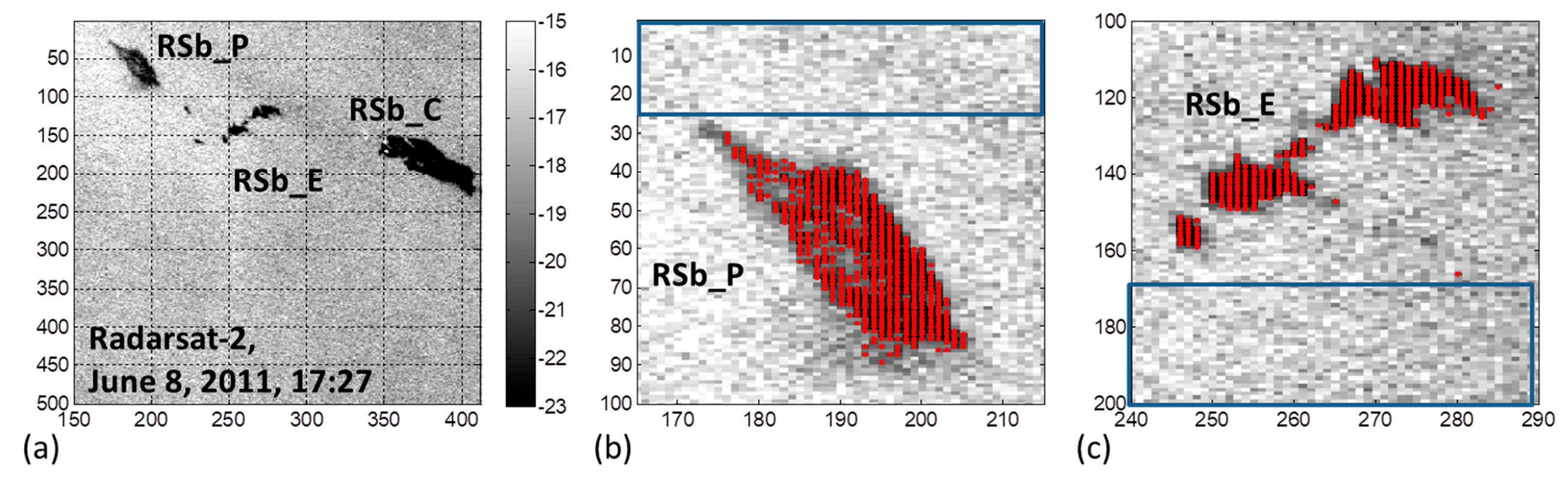
This study is based on oil spill data collected during oil-on-water exercises conducted by the Norwegian Clean Seas Association for Operating Companies (NOFO) in the North Sea (centered at 59°59′N, 2°27′E) in 2011 and 2012. Different substances—crude oil, oil emulsion, and plant oil—were released onto the sea surface (Figure 1a) for the purpose of equipment and procedure testing, thereby providing unique opportunities to collect remote sensing data of oil spills and look-alikes. Four RS and two TS images were acquired during these oil-on-water exercises. Data were collected by RS in Fine quad-pol mode, and by TS in Stripmap mode. The properties of the studied SAR scenes, including wind conditions and spills, are presented in Table 1 (in general, slicks were observed at low to moderate wind speeds 2–6 m/s and low wave heights < 2 m). More detailed information can be found in previous studies [8,21,37]. We follow the notations used by Skrunes et al. [21] in denoting the TS scenes as TSa and TSb, and the RS scenes as RSa, RSb, RSc, and RSd (Table 1). Since several releases of emulsion occurred in 2012, we numbered them from 1 to 6.
The images span the incidence angles from 27° to 49°. Two RS and two TS images were co-located in time and space. Two RS images (RSb and RSd) with an SNR within the slicks for the HH channel () of more than 5 dB were used in work [35]. We used the HH channel of an image for the calculation, since the HH channel has lower NRCS than the VV channel. The newly included RS images (RSc and RSa) had values of 2 and −3 dB, respectively, which may be considered low and extra low SNRs. One of the TS images (TSa) acquired at incidence angles around 28° has a good of 8 dB. Another TS image acquired around 41° has a low of 0 dB.
The details of the oil releases are presented in Table 2. The plant oil was Radiagreen EBO (a monoalkyl ester of an oleic acid produced from vegetable oils) previously used for simulation of biogenic slicks [8]. The behavior of Radiagreen EBO differs somewhat from the expected characteristics of a natural biogenic slick [43] and may not be a perfect proxy, but is still useful for comparison to mineral oils. The emulsion released in the 2011 exercise was Oseberg blend crude oil mixed with 5% IFO3801 with a water content of 69%. An emulsion of the Oseberg blend was also released during the 2012 exercise, with an initial water content of 58% [21,37]. The crude oil was evaporated Balder oil. Based on the lab analysis of this oil type [8,44], this oil was expected to produce stable emulsions with a water content of 21% under wind speeds of 2 m/s and 55% at 5 m/s. Further information on the oil properties is provided in previous studies [8,21,37].
The question of oil film thickness plays an important role in the applicability of the polarimetric analysis proposed here. The polarimetric method proposed in [37] was developed for sufficiently thin oil films in comparison to the penetration depth of a radio wave. The average film thicknesses of the oil released during oil-on-water exercises in 2011 and 2012 were estimated, assuming all the released oil was uniformly distributed on the surface. The slick areas were calculated using available SAR images. For separation of the slick area from clean water, we calculated the level of average signal for waters neighboring slick and marked image pixels, which had signal level less than 0.4 (linear scale) of that of water. VV polarization (8 × 8 multi-looked) images were used since they have a higher contrast between the slick and water. An example of this area calculation is demonstrated in Figure 1b,c.
The results for all the slicks are presented in Table 2. According to these estimates, the mean thicknesses of the emulsions were in the range of 9 to 23 μm and the crude oil thickness was 6 µm. Thus, in general, the emulsions had a greater average SAR-sensed thickness than crude oil. The plant oil spills had an average estimated thickness of 0.3 µm for slicks that had been weathering and spreading for 13–14 h. Of cause, a film having such a thickness of 0.3 µm is not a very good proxy for natural monomolecular films having thickness of several nanometers. Nevertheless, the value of 0.3 µm is 1–2 order less than that for mineral oils. The thickness of the RSa_P film, after only 2 h on the surface, was estimated to about 3.5 µm. We assume that this 2 hours’ time was insufficient for stabilization of the final plant oil film size and corresponding thickness.
These conclusions are in agreement with the results of studies devoted to the testing of oil properties at sea [45,46,47,48,49], which showed that oil spills at sea formed a comet-like shape, where three zones can be distinguished: (1) extensive areas of silver sheen and rainbow-appearing film (i.e., 0.04 to 5 μm), (2) large areas of the film with visible near-infrared reflectance and thermal-infrared emittance characteristics, corresponding to the Bonn Agreement’s metallic Code 3 [50] with a thickness range of approximately 6 to 70 μm; and (3) oil emulsions, most commonly in the form of strands, having a thickness of 1 mm and greater. According to data published by Daling et al. [45] acquired during NOFO-1994 trial with oil slicks of Sture Blend North Sea crude and 3 hours of weathering at moderate sea state with wind speed varying between 8 and 12 m/s and about 2.5 m significant wave heights, the same comet-like shape consisting of three zones was observed [45]: (1) ~85% of the slick area was a sheen with film thickness less than 1 μm, which contained 2%–3% of the mass, (2) ~15% was 5–100 μm thick, containing 10%–15% of the mass, and (3) 1%–2% of the area, containing 80%–85% of the mass, was a thick (2–9 mm) emulsion.
Therefore, the results for all the film thicknesses presented in Table 2 agree with previous works [45,46,47,48,49]: the most part (according to some of the cited papers, more than 98%) of the slick area for a mineral oil spilled on the sea surface should consist of the film less than 100 μm thick, and only a tiny part of the slick area should have a film thickness greater than 1 mm. We take this statement as a key point for the subsequent analysis.
3. Polarimetric Approach
Our polarimetric approach is based on the NRCS model of the dual co-pol scattering from the sea surface developed in Kudryavtsev et al. [34], which considers three polarization terms: (1) is the conventional two-scale resonant Bragg scattering from the short gravity-capillary wind waves (i.e., Bragg waves superposed on long waves; the subscript p denotes either H (horizontal) or V (vertical) polarization), (2) is the non-polarized specular Kirchhoff reflection from the slopes of long waves, and (3) is the non-polarized scattering due to a non-resonant scattering from the rough surface patches (RSP) caused by wave breaking. The NRCS for co-pol channels is thus defined as:
The main details of the NRCS model are given in Appendix A. The main elements and processing steps of the proposed polarimetric approach are described below.
3.1. Step 1: Calculation of the Resonant and Non-Resonant Parts of Signal
When using the dual co-pol sensing, we only have two sensing channels; so, the range of incidence angles has to be limited when one of the signal sources (reflections from slopes of long waves) becomes negligible compared to the others. For SAR observation conditions of mineral oil slicks, this corresponds to angles greater than ~27°. This is the first limitation of our method. However, the other dual co-pol methods based on NRCS models also impose a similar restriction [14,28] to remove unnecessary uncertainties in the form of reflections from slopes of long waves. According to the definition of the NRCS model [34], the following expressions for the resonant and non-resonant parts of the backscattered signal are obtained:
where . We omit here the dependence on slopes of long waves, therefore, Equations (2) and (3) are valid to the first order of the slopes of long waves.
3.2. Step 2: Elimination of the Incidence Angle Dependence
The dependence of and on the incidence angle can be eliminated by introducing the damping factors and for resonant and non-resonant signals, respectively, relative to their values for clean water:
where and are the slick intensities within the dark patch, and and are the clean water normalization parameters, which are mean intensities for the part of the SAR image not containing the dark patch (at the same incidence angle).
In the approximation of a radio thin slick, the variations in the coefficients and due to the oil dielectric constant may be ignored. Therefore, for radio thin slicks, the damping factors and are proportional to suppression of short gravity-capillary waves in the slick, and to a suppression of the fraction of sea surface area covered by RSP in the slick, respectively, i.e.,
where and are the spectra of short gravity-capillary waves in the slick and in the clean water, respectively, which is the same for and . The normalizations in Equations (2)–(6) enable the removal of most of the dependency on and emphasize the dependence of parameters and on the film thickness , the film mechanical properties (for example, elasticity ), and the weather conditions such as wind speed, temperature, etc. (hereinafter, the parameter denotes all the weather conditions). The remaining dependence of and on is contained in the Bragg wave number , which is included in the definition of the spectrum [34]. The wave breaking fraction , sensed by the radar, should depend on the frequency band that enters into Equation (15) through . The frequency band also enters into .
3.3. Step 3: Elimination of the Unknown Oil Thickness Variations
A scattering of and points are dependent on the variations of film thickness , which are unknown priory. To exclude the film thickness from Equations (5) and (6), we considered the formal expansion of and in the Maclaurin series on the film thickness variations :
where is the second- and higher-order terms of .
Following the idea to remove the unknown we propose the multi-polarization parameter:
where
is the relative change in the intensity of the wave breaking in the slick and
is the relative change in the intensity of the Bragg ripples in the oil slick [35].
Thus, from Equations (7)–(9) for the radio thin slicks (see Appendix B), the parameter should be sensitive mainly to the information about the slick type (the film elasticity ):
as well as weather conditions, temperature, etc., which are not addressed in this paper. By the definitions in Equations (7) and (8), can not be totally removed, but can be excluded from the 0th order of the , which is expressed by the first term in Equation (12), shifting dependence on to the next order terms defined by in Equation (12). Due to the normalizations described by Equations (7)−(12) and known relationships to NRCS theory [34], the should have some predictable dependence on the Bragg wave number , which, in turn, incorporates the dependence on the radio frequency band and incidence angle.
3.4. Step 4: Getting StatisticallyReliable Polarimetric Parameters
Due to the random nature of the and values, the pixels of and form a two-dimensional probability density distribution . For operational and analytical purposes, it is convenient to have a quantitative value derived from the polarimetric distribution . Therefore, this distribution was integrated using new arguments, and . As previously mentioned, by the definition in Equation (12), the first argument, , is weakly dependent on the film thickness, whereas the second, , depends strongly on the film thickness. for clean water, and for thick slicks. As the two-dimensional distribution can be averaged over some normalized damping , related to the film thickness variations . This step helps exclude from the polarization parameter impact of the film thickness variations and to produce a more statistically significant estimate. Accordingly, the one-dimensional probability density distribution related only to the polarization parameter , can be obtained as the integral:
The lower limit of integration , which separates the area of the slick from the clean water, was set to 0.6 based on various test calculations. In the following step, for the one-dimensional distribution , the mean and its standard deviation ( and , respectively) were calculated by applying the centroid method [51]:
and
Here, according to the centroid method practice, the cut-off of ½ the maximum of the histogram height was applied to separate the peak from the surrounding continuum, i.e., the summation is performed over the indices , for which is greater than ½ the maximum of .
This final , derived from the dual co-pol channels according to the presented technique, is expected to be sensitive mainly to the information about the slick type (the film elasticity ):
and, secondary, to weather conditions denoted as , and sensor and SAR scene parameters and , which are known or may be estimated (concerning ) from the SAR scene. Ideally, an impact from these secondary parameters to and channels may be predicted using the Kudryavtsev et al. approach [34] to the NRCS theory, or in the framework of the other approaches, describing the non-resonant scattering term analogous to . Practically, the quality of such predictions will depend on the quality of used estimations of the NRCS. In our work, we concentrate our efforts on investigating the potential of the parameter to separate different slick types and to relate various SAR observations of slicks collected in different frequency bands.
3.5. Data Instrument Noise Correction
The instrument noise floor, namely the NESZ, which is a measure of the sensitivity of a given SAR, has a great impact on the sea slicks detectability by the SAR [3,14,29]. The NESZ is caused by a number of factors [17,29], e.g., the antenna pattern, the power of the transmitted pulse, the receiver noise, the bandwidth, the analogue–digital converter quantization noise, and, to a negligible extent, processing noise (for TS data, there was a NESZ dependence on the preprocessor version also before the version 4.7 [52]). Considering that the NESZ is an additive noise, the SAR data specifications [17] and the practical use of the low backscattered signal [12,13] require removing the NESZ from the data as follows:
where and are the normalized backscatter derived directly from the radar brightness and contaminated by the NESZ; and are the NESZ for vertical and horizontal polarizations, respectively (for RS data, only one value of NESZ is provided, and and are hence equal); and and are the NRCS cleaned from the NESZ. and measured by the radar can be lower in amplitude than the NESZ. This problem has been addressed in [3,8,21]. This is an important point in our analysis. Usually, in previous studies, the data with low SNR within the slick ( < 5 dB [8,21,35])
were discarded from the consideration to prevent unreliable estimates (here was chosen since usually for water ).
Some of the drawbacks of using is that slicks often have small spatial scales, and this is why the value depends on image multi-looking and smoothing. We will see this in the examples in the next section. In data processing, we use a 300 m × 300 m scale for SAR image smoothing. Accordingly, values will be given for this condition. Another disadvantage of is that on the same SAR image, slicks with different brightness contrast correspond to different . Moreover, more contrasting and, therefore, more convenient for research, slicks will have worse than a slick with lower contrast (and less convenient for research). Therefore, to characterize the noise level relative to the background of clean water, the value defined on for clean water will also be given for the image.
4. Results of the Dual Co-Pol Data Polarimetric Processing
In the processing results presented below, we start with an example of RSb and RSd data that have a relatively good of about 5–11 dB. These images will be used as a reference case. Next, pairs of RS and TS images obtained with a difference of about half an hour will be presented, some of which have a relatively bad below 0 dB. Their example will show the effect of SNR on processing results. The most important technical details of the processing will be given in the following subsections as part of the processing results. It is noteworthy that to ensure the most identical conditions when comparing the processed data, the processing was completely unified for all slicks and images (RS or TS), which means that the same 2200 m × 2200 m size of processing areas around the slick and the same 300 m × 300 m scale of the SAR image smoothing were kept constant for all the slicks and images. The only difference in the processing of RS and TS images was that 8 × 8 multi-looked SAR images were used as RS input data, and 16 × 16 multi-looked images were used as TS input data. Such initially multi-looked images were used to save computer storage space and to speed up the processing. Different multi-looking for RS and TS images was applied for reasons of approximately equalizing the sizes of multi-looked pixels of RS and TS images, which in the original images differed by more than 2 times (Table 1).
4.1. Radarsat-2 2011 and 2012 SAR Images with Good SNR
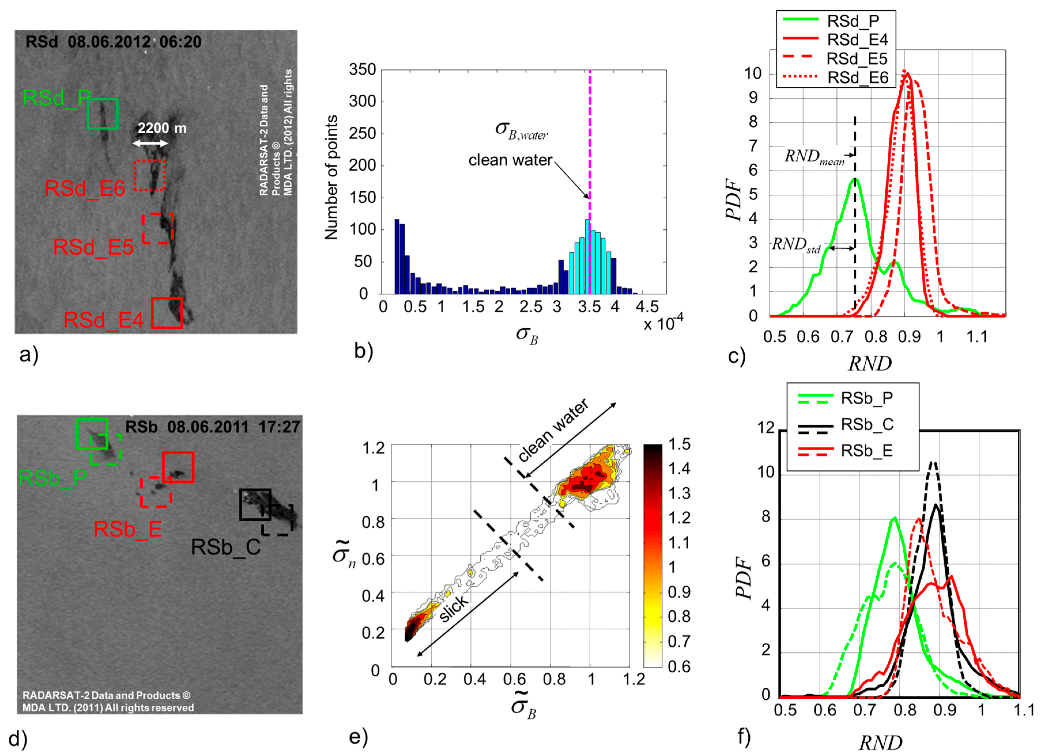
In this subsection, on the example of the RSb and RSd images, we demonstrate the polarimetric processing presented in the previous section. Figure 2a shows a subscene of the RSd imageacquired on June 8, 2012, 06:20 UTC that contains three emulsion slicks (RSd_E4, RSd_E5, RSd_E6) and one plant oil slick (RSd_P). The corresponding selected processing areas are indicated by squares having a 2200 m × 2200 m size. Each such area contains the point of the maximal signal suppression within the slick and covers different parts of the slick, and contains both slick-covered regions and clean water. The square form of the processing area is chosen to not depend on the slick orientation. The size of the processing area of 2200 m was chosen considering the fact that the slick area had a width of 500–800 m and length of a few kilometers. Therefore, the main part of the processing area contains clean water, whereas the minor part contains the slick. This is done in order to obtain a well-pronounced peak near clean water (Figure 2b) and to implement the robustness of automatic determination of and needed for the accurate normalization in Equation (4).
Figure 2b illustrates the process of the automatic determination of the value of by applying the centroid method, similar as in Equation (14), to the RSd_E4 processing area. The light blue color marks the part of the -distribution used for calculation. The same procedure was applied for .
After finding and for each point within the region, we calculated the damping factors and using Equations (5) and (6), and then the density distribution shown in Figure 2e. The area with the lower limit of integration in Equation (13) that is marked as ‘slick’ in Figure 2e was used for calculation of the one-dimensional probability density function of the slick RSd_E4 (Figure 2c). Based on , values of and were determined for this slick (Table 3). The other slicks on RSd were processed similarly. The three emulsion slicks (RSd_E4, RSd_E5, and RSd_E6) lay close to each other and are non-distinguishable in terms of varying from 0.892 to 0.930 and varying from 0.018 to 0.024. The plant oil slick RSd_P having = 0.759 and = 0.032 is well distinguishable from the emulsion slicks.
The same processing was performed for slicks on the RSb image acquired on June 8, 2011, 17:27 UTC (Figure 2d). Additionally, to demonstrate the robustness of the processing when applied to various parts of the same slick, we also processed two different parts of the same slick. Results presented in Figure 2f and Table 3 show that the emulsion and crude oil slicks coincide in terms of varying from 0.882 to 0.888 and varying from 0.024 to 0.026. The plant oil slick RSd_P having = 0.782 and = 0.029 is well distinguishable from the mineral oil slicks.
These scenes (RSb and RSd) highlight the good discrimination ability of our method between mineral oils and the plant oil. Additional conclusion is that the processing areas that contain less contrasting parts of the slick and do not contain the point of the maximal signal suppression within the slick do not differ in terms and from areas with more contrasting slick parts. However, a decrease in the contrast of the slick leads to a less clear differentiation of it from other slicks. In this sense, of course, it is necessary to use the most contrasting parts of the slick.
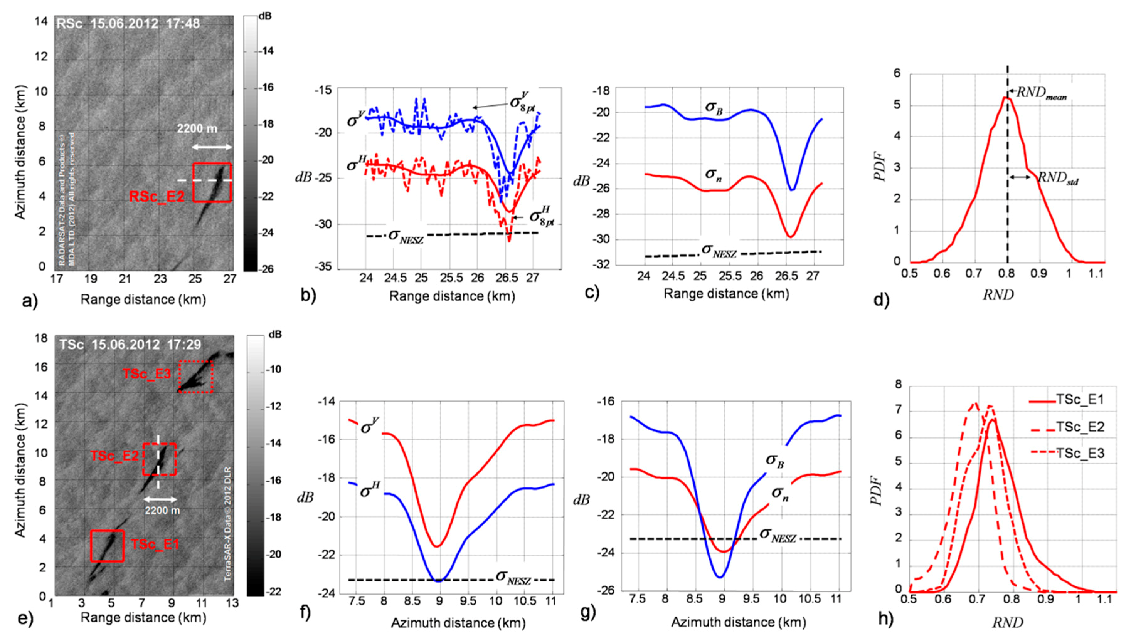
4.2. Pair of Near-Coincident Radarsat-2 and TerraSAR-X SAR Images Acquired June 15, 2012 (Evening)
The near coincident TSc and RSc images were acquired on June 15, 2012, 17:28 and 17:48 UTC, correspondingly. Both of these scenes were obtained at large angles of 41° (TSc) and 49° (RSc), when the manifestation of noise in the data becomes noticeable. The RSc scene has the of 2 dB (Table 1), therefore, the noise may be considered here as partially influencing the signal. The TSc scene has the of 0 dB, therefore, the noise here is at the same level as the signal.
The results from processing the emulsion slick RSc_E2 visible on the RSc image are presented in Figure 3a–d. Figure 3a shows a subscene of the image and the selected processing area. Figure 3b shows the cross-sections through the slick (at the position indicated by the white dashed line in Figure 3a) of the co-pol channels and in comparison to the NESZ. The dashed lines and represent the input 8×8 multi-looked signal (shown in Figure 3a), while the fat lines and represent a 300 m × 300 m smoothed signal, which is used further in the processing. Figure 3b illustrates the effect of the smoothing that reduces the speckle beats.
The Hanning window with 300 m half-width in each direction (range and azimuth) was applied for the smoothing. Therefore, for the RSc scene with an initial pixel resolution of 6.26 m × 5.11 m (Table 1) and applied 8 × 8 multi-looking, the smoothing Hanning window was 12 × 15 (range and azimuth, respectively), which corresponds effectively to a multi-looking of 48 range pixels × 60 azimuth pixels. An effect of 48 × 60 multi-looking, in this case, results in a reduced radiometric error equal to 0.08 dB for the estimated averaged level of the signal (the value of error in decibels is calculated as . Such reduced error leads to a reduction of the blur of of the slick. The cost of the smoothing is the reduced resolution of the final image. Another effect of smoothing is the slightly biased extreme (minimal) values of smoothed and . The unsmoothed extremes of and can lie −3 dB below the smoothed extremes since the central part of the slick with a minimal backscatter value is mixed with greater values on the 300 m scale in the range and the azimuth.
Our tests with different smoothing window sizes ranging from 50 m to 500 m showed that a half-width of 300 m provides a reasonable trade-off between robustness and spatial resolution when processing oil slicks. Figure 3b shows that the cross-slick width (in the range direction) is about 500–800 m, whereas Figure 3a indicates that the length of the slick extended along the azimuth is about 3500 m. Therefore, the chosen smoothing size of 300 m is two times less than the slick width and 10 times less than the slick length.
The NESZ of this part of the RSc image lies near −31 dB (Table 3) which is typical for RS quad-polarization mode [16]. Due to the low backscattering in the slick, the co-pol signals and are close to the noise floor, particularly in the horizontal polarization channel . The for within the slick is 2.3 dB for the 300 m smoothing. The components and are shown in Figure 3c. The non-resonant part within the slick is only 1.3 dB higher than the NESZ. For such noise conditions, a relatively wide, in comparison to RSd and RSb results, of the RSc_E2 slick (Figure 3d) with 0.047 and 0.802 was determined (see Table 3).
The near coincident TSc image was acquired 20 minutes before the RSc image. The subscene shown in Figure 3e contains three slicks: TSc_E1, TSc_E2, and TSc_E3, following notations of Skrunes et al. [21]. TSc_E2 is the same emulsion slick as in the RSc image (RSc_E2). Rectangles containing slicks and clean water around them delimitate three corresponding processing areas. The cross-sections in Figure 3f,g show values of , and in comparison to the NESZ for the TSc_E2 slick, at the position indicated by the dashed line in Figure 3e. The NESZ is −23.3 dB. The minimum is −0.1 dB below the NESZ (Table 3, TSc_E2 slick). Correspondingly, minimum is −2.0 dB below the NESZ, and the minimum is −0.7 dB below the NESZ. Figure 3h shows for the three emulsion slicks (TSc_E1, TSc_E2, and TSc_E3), which lay close to each other and are non-distinguishable in terms of , varying from 0.686 to 0.753, and , varying from 0.032 to 0.037 (Table 3).
It is worth to note the following fact here: for the more noisy TSc_E2 case ( = −0.1 dB) 0.04 is less than 0.05 for the less noisy RSc_E2 case ( = 2.3 dB). We suppose that such an effect can be explained by different radiometric errors of RS and TS images related to the smoothing of these images having different initial pixel sizes. For TSc scene with an initial pixel size of 1.34 m × 2.25 m and 16 × 16 multi-looking, the 28 × 17 smoothing Hanning window was applied to obtain the resulting smoothing of 300 m in each direction. In this case, the smoothing results in an error of 0.025 dB for the averaged signal level (see the corresponding expression for in the previous subsection) in comparison to 0.08 dB in the case of RSc.
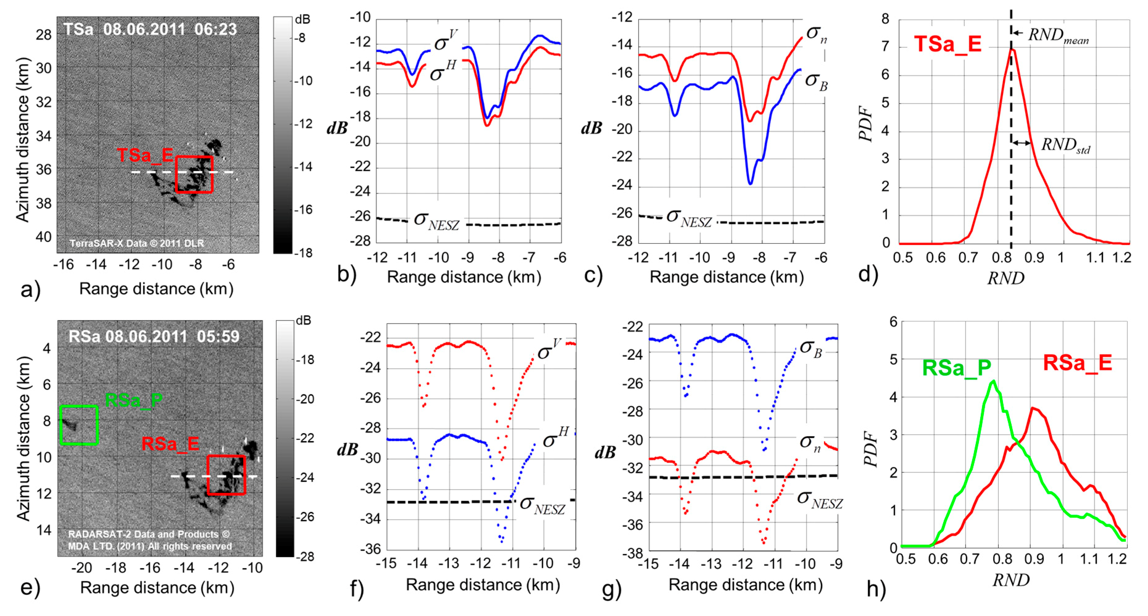
4.3. Pair of Near-Coincident TerraSAR-X and Radarsat-2SAR Images Acquired on June 8, 2011(Morning)
Similar processing was performed for the TSa and RSa images acquired on June 8, 2011, morning, as shown in Figure 4. The time difference between the image acquisitions is 24 minutes (RSa acquired at 05:59 UTC and TSa at 06:23 UTC). Therefore, the images depict the emulsion slick at almost the same weather conditions (Figure 4a,h). The plant oil slick was outside the area of the TSa scene.
The cross-section in Figure 4b (whose position is indicated by the white dashed line in Figure 4a) shows the NESZ and the backscatter values of the co-pol channels and for TSa_E. The NESZ in this part of the TSa image lies near −26.6 dB. The minimum for the channel is 8 dB (Table 3). The cross-section of and for the TSa_E slick are shown in Figure 4c. Here, the non-resonant signal in the clean water is about 2 dB greater than the Bragg signal . This occurs due to the relatively small incidence angle of about 28° and the exponential growth of the non-resonant signal with decreasing angle [34]. The minimum is 7.1 dB higher than the NESZ but the Bragg signal in the slick falls closer to the NESZ (2.4 dB above the NESZ). At such SNR conditions, results in a narrow distribution (Figure 4d) with a small peak width of 0.023. The value is 0.840 for the TSa_E slick.
For the RSa_E slick (Figure 4e), the minima and lie close to the NESZ of −32.8 dB and is −2.7 dB (see Figure 4f and Table 3). The minimum of is close to the NESZ as 1.8 dB and lies −4.7 dB below the NESZ (Figure 4g). The low signal-to-noise ratio results in much noise and a diffused distribution of (Figure 4h) with a large peak width of 0.063. The value is 0.915 for the RSa_E slick. Similar difficulties with noise are observed for the processing of the plant oil slick RSa_P: the diffused distribution in Figure 4h and the large peak width of 0.048. The value is 0.81 for the RSa_P slick. Having such and the distributions of the slicks RSa_E and RSa_P are significantly overlapping making their distinguishing not easy: the distance between their centers (0.915 − 0.81 = 0.105) is less than the sum of their halfwidths (0.063 + 0.048 = 0.111).
5. Summary of the Polarimetric Processing
5.1. Summary Diagram for the RND Mean
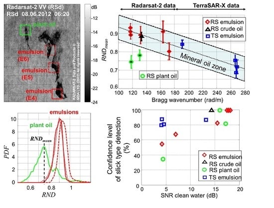
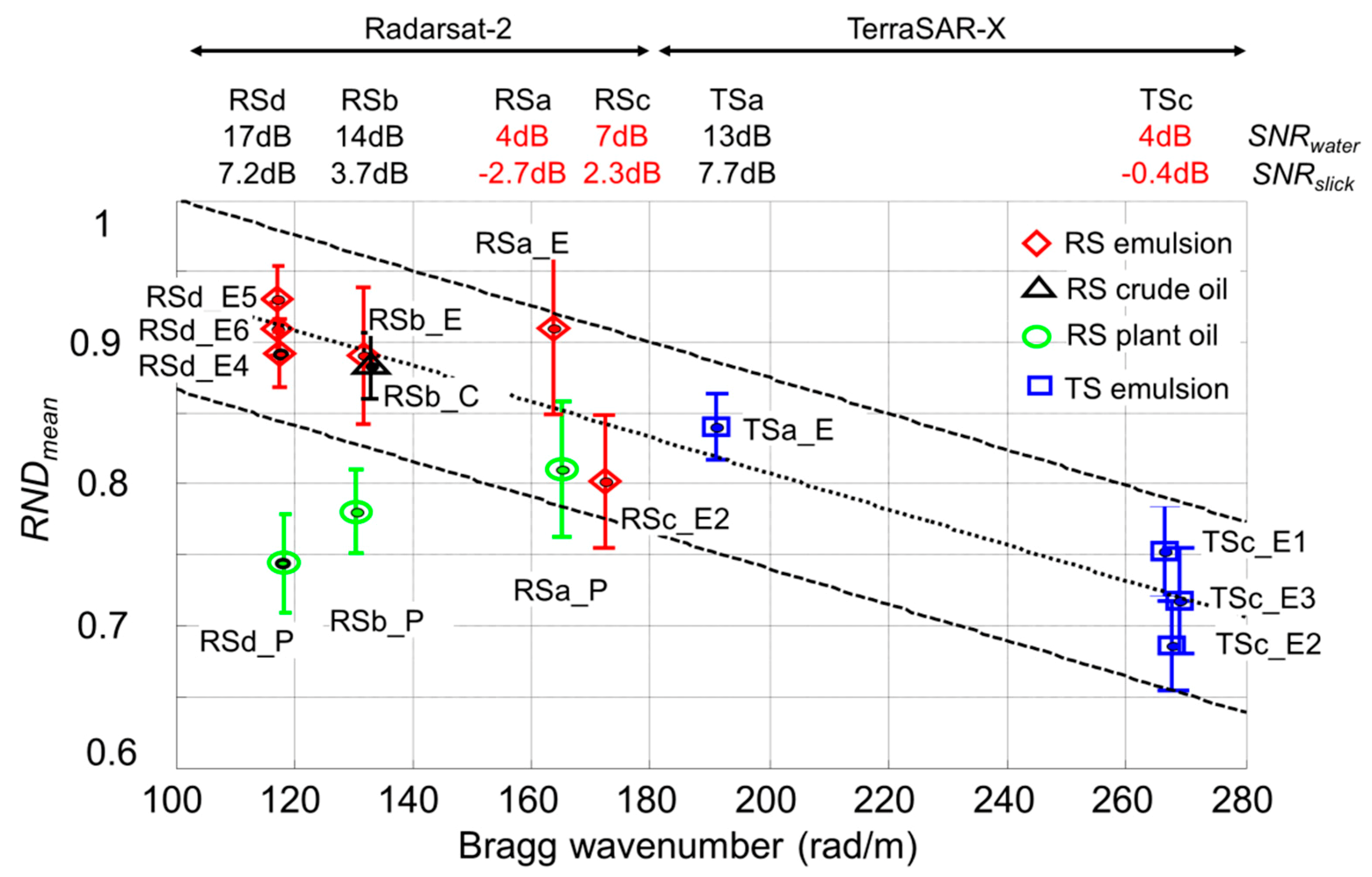
A summary of the results of all the processed slicks from the RS and TS images is shown in Figure 5. Here and below, where it is not noted otherwise and to maintain the same number of points per slick, we only consider the processing area with the highest contrast for each slick (for the case of Figure 2e, which is marked by the solid line). Since these SAR images were obtained in different frequency bands (C- and X-bands) the was plotted as a function of the Bragg wave number (as it was applied in [23]), which includes both the sensor frequency, through , and the incidence angle, through . RS data lie on the left of 180 rad/m, TS data are on the right of 180 rad/m. Scene names, and are shown at the top, opposite the corresponding Bragg wave numbers.
The of mineral oils (crude oil and its emulsions) obtained in C- and X-bands correlate well amongst themselves locating along a line, which is monotonically decreasing from small to large Bragg wave numbers. The dotted line in Figure 5, calculated using the least square method (the root-mean-squared residual is 0.026), shows the most likely position for mineral oil . It behaves as:
The results in Figure 5 indicate that the parameter may describe in some generalized way the properties of slicks when sensing in different frequency bands and at different incidence angles.
As mentioned earlier, the parameter defines the ratio of the suppression of wave breakings vs. capillary-gravity ripples in slicks. The monotonic decrease of the parameter for mineral oils from small to large Bragg wave numbers indicates that the shorter ripples are suppressed more intensively than the longer ripples in comparison with the suppression of wave breaking. This observation is in accordance with the results of works [22,23].
The dashed lines in Figure 5 delimit upper, , and lower, , boundaries of within which the values of mineral oil lay together with their . These upper and lower boundaries were defined based on presented in Equation (19) plus/minus the two averaged values of calculated over all mineral oil in Figure 5. This averaged was 0.034 for our data. Therefore, the corresponding upper and lower boundaries for of mineral oils are:
This choice for the mineral oil boundaries is one of several possible variants and can be corrected in the future. Using the Equation (20) definition for boundaries, within which the mineral oil has a high probability of occurring, we propose a method through which the reliability of the slick type detection could be estimated.
In Figure 5, the points for two of the three plant oil slicks lay outside (together with their error bars) of these mineral oil boundaries. Unlike RSb_P and RSd_P, the RSa_P plant oil falls into the zone for mineral oils. For this case, it should be noted that, according to estimates, the RSa_P slick should not be considered fully outstretched, therefore, the RSa_P film has an order of magnitude greater thickness (Table 2) than RSb_P and RSd_P films. For this reason, the RSa_P slick should be considered as a not reliable plant oil slick case.
Additionally, the RSa image has the worst SNR level (= −2.7dB) and the closest to the NESZ floor the non-resonant part (see Figure 4g and Table 3). An analysis of the behavior of slick versus , presented in Table 3 for oil spills visible on RS and TS images, shows that, overall, the worse the signal-to-noise ratio, the wider the standard deviation, which is more or less predictable in advance. For this noisy RSa scene, the distributions produce the most diffused estimates for of all scenes. Therefore, the RSa_E point does not exactly lie within the mineral oil boundaries (Figure 5). Considering its error bar, we could estimate that almost half of its distribution lies outside the mineral oil boundaries.
The experimental data used in this work allowed us to study the behavior of the parameter at C- and X-bands at various incidence angles ranging from 28° to 49°. This covers a significant part of the operating range of SAR angles, which range from 20° to 60°. Particular attention was paid to the most complete unification of data processing (C- and X-bands) from different satellites (RS and TS) to obtain data suitable for comparison under the most similar conditions. We found that the mineral oil samples (crude oil and emulsions), observed at both these frequency bands and all these incidence angles, form a coherent mineral oil zone on the plane created by the parameter and the Bragg wave number.
According to Equation (19), the average position of the parameter changes by ~30% when the Bragg wave number is changing on 100% (within the range of 117 to 267 rad/m). These changes in the parameter can be related to both changes in the proportions of suppression of resonant ripples and non-resonant wave breaking with changing incidence angle or the carrier frequency of the radio wave, as well as an increase in the relative noise fraction in the data, which occurs with increasing incidence angle, as discussed by Nunziata et al. [29]. The values of the RSd_E and TSa_E points were obtained at approximately the same of 7–8 dB (Figure 5) and close angles of 28°–31°, but at different frequencies that differed by 7% (Table 3). The is greater for C-band. A similar difference in , by about 10%, was observed for the points RSc_E2 and TSc_E2 obtained at of 0–2 dB and angles of 41°–49°. Thus, we preliminarily conclude that switching from the C-band to the X-band, ceteris paribus, causes a 7%–10% decrease in . This result supports our hypothesis that the parameter can effectively describe oil slick properties within some range of radar frequencies.
Accordingly, the remainder (30%) of changes of about 20% can be attributed to the influence of the data noise level with increasing incidence angle, as well as the influence of wind direction and wind speed spread from 2 to 6 m/s according to ship data. These factors should contribute to the spread of data, and, in theory, their correct accounting should help with further improving the mineral oil diagram in the future.
An important parameter for separating different types of slicks is , which determines the width of the mineral oil zone and the dispersion width of each individual peak. In this study, on the basis of preliminary tests, to achieve optimal values, we averaged the images with a window of 300 × 300 m. For some problems, this choice of averaging is optimal; for others, other averaging will be necessary. The averaging value should affect all parameters associated with RND: , , , and . This issue also requires further study.
One drawback of the proposed mineral oil diagram is that for the formation of the mineral oil zone, only 11 experimental points of mineral oil samples were used, which is a statistically small number of points, so further confirmation of this hypothesis using experimental data is required. In our current study, for the formation of the mineral oil diagram, only 100% experimentally reliable points were consciously used, with known substances and their properties, with known weathering time and known spilled volumes. The thickness of the films was also controlled by available means. To form a mineral oil diagram, in the present study, the mass of images supposedly including mineral oil spills (but not 100% reliable) with dark spots, unknown weathering times, and unknown spilled volumes was deliberately excluded; therefore, film thickness was less evaluable. In the next stage of research, we plan to include these less reliable data in the processing.
5.2. On Confidence Level for the Slick Type Discrimination
According to the definition of mineral oil boundaries, it becomes possible to assess confidence levels for the slick type discrimination. To do this, one can use the value based on the calculation of the fraction of the number of points of the distribution for the tested slick, which fall inside the mineral oil boundaries and . However, as shown in the examples in Figure 2c of two-dimensional distribution , the transitional part of between the slick and clean water (corresponding to lower signal suppression contrasts near the lower limit of integration in Equation (13)) takes part in the formation of the distribution. As a result, a relatively wide the surrounding pedestal associated with this diffused transition zone may arise in . Since, at low contrasts of signal suppression, the characteristics of clean water, and not the film itself, begin to play an increasingly important role, respectively, the surrounding pedestals, calculated for different slicks, can intersect over fairly wide limits (for example, see Figure 4h). For this reason, we propose that, in order to determine an appropriate confidence level, it is better to use only points lying in the vicinity of the maximum at a level above ½ the maximum.
Similarly to the centroid method practice applied in Section 4 (Equation (14)), confidence levels (for mineral oil) and (for plant oil) may be defined as follows:
Here, the summation is performed over the indices and , for which is greater than ½ the maximum of . Additionally to this condition, the indices mean that the points lie within the mineral oil boundaries: ; correspondingly, the points lie below these boundaries: .
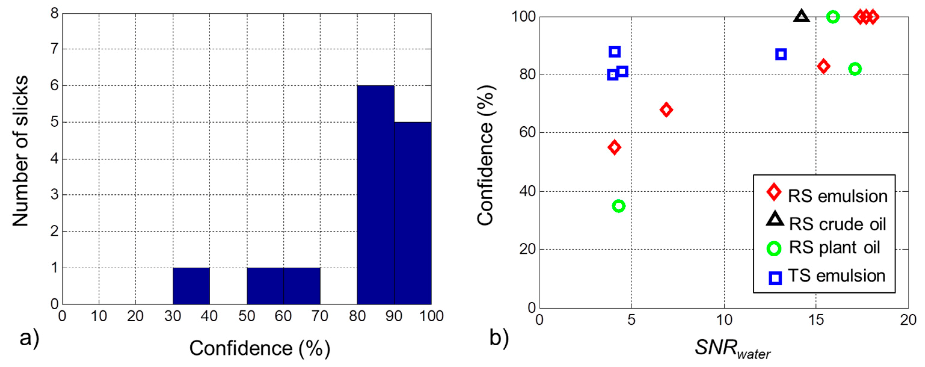
In all cases (except for the RSa scene with the bad SNR and the low contrast part of the RSc_E2 slick), the confidence level for the mineral oil slicks being detected as mineral oil was higher than 68% (Table 3). The confidence level, , for the plant oil slick to be detected as plant oil (except in the noisy RSa scene) varied from 82% to 100%. Figure 6a shows the distribution of the resulting confidence values for both the mineral oils and plant oil. As mentioned above, only the results for the higher contrast part of the slicks are presented here. Of the 14 slicks, 11 of 14 (i.e., 79%) are situated properly with a confidence level higher than 80%; and 12 of 14 (i.e., 86%) are situated properly with a confidence level higher than 68%. These numbers were produced using the determination of the mineral oil boundaries given by Equation (20). Using a different method of performing this determination will change the boundaries, and will accordingly produce slightly different results. We assume the results will only be ‘slightly different’, since the main principle of separating the different types of slick remains almost the same, by separating mineral oil from plant oil slicks by any suitable line.
Figure 6b shows the dependence of the confidence level on . In general, for the RS data with better than 7 dB ( better than 2 dB), the confidence level is greater than 68%. TS data demonstrate better behavior: they have a confidence level better than 80% until is about 4 dB. The noisy RSa scene with the about 4 dB and a of about −3 dB produced correspondingly bad confident results: nearly 55% for the mineral oil slick and nearly 35% for the plant oil.
The reasons for the better result of TS data processing, compared to RS, we see in the smaller radiometric errors of the smoothed TS images in comparison to the smoothed RS images due to the averaging of more points for TS images for the same spatial averaging (which was discussed in the Section 4.2). Therefore, maintaining an identical confidence level for both TS and RS processing results, finer geometric details can be processed with finer resolution data. There is a trade-off between the initial data resolution, the signal-to-noise ratio, the confidence level of the results, and the geometric scale of the studied event, which has to be studied in future works.
6. Discussion
Both expressions (for the ripples, , and the wave breaking, ) depend on weather and geometrical conditions during SAR observation, as well as on the dielectric constant of seawater, which, in the presence of thick (more than 1 mm) oil films, can strongly affect the reflection results. Our proposed method allows working with only thin films (less than a fraction of one millimeter); therefore, consideration was paid to checking the actual thickness of the experimental films visible on SAR images. This issue is crucial because, in the absence of direct measurements or other data about the thickness, any assumptions can be made, and accordingly, mutually exclusive polarization models of scattering from oil slicks can be applied. According to our experimental data, based on the known volumes of the spills and their areas and data on the distribution of the film thickness for similar spills [45,46,47,48,49], we concluded that the film of the experimental spills used in our work is thin (less than 0.1 mm in average), so our approach can reasonably be applied.
If no such experimental data are available upon which a conclusion about the film thickness can be drawn, then the questions remain open: is it correct to apply the method (polarization parameter ) for an unknown film thickness: How much can the results of this method be trusted? In any of similar studies, the question of the thickness of oil films will remain key for correctly choosing a model that describes polarization scattering from the oil film, and, for successful progress, it will have to be determined.
Under fulfilling such restrictions (angle greater than ~27° and films thinner than 0.1–0.3 mm) and having two channels for dual co-pol sensing according to the NRCS model [34], it is possible to 1) unambiguously separate two signals (ripples and wave breaking), then (2) reduce the majority of dependence on incidence angle, and (3) form the polarization parameter on this basis, and, accordingly, to concentrate on studying the behavior of the parameter of varying of the sensing frequency (C-band and X-band), weather conditions (wind speed and wave height), and noise level.
Notably, we neglected the possible effect of the tilt angles of long waves on the final results in our consideration, assuming their minor effects on the backscattering and polarization coefficients in comparison to the incidence angle influence at moderate seas. A summary of the estimated effects of the discussed parameters on possible variations in the mineral oil is provided in Table 4. In general, further detailed analysis of the data is required for the most of the items in Table 4 (for example, to determine the most appropriate wind speed for each SAR image, as well as the tilt angles, related to longer waves on the ocean surface), which we plan to complete in the future.
Regarding the influence of the SNR, the data with SNR of 4–17 dB for clean water (respectively, from −3 to 11 dB for slicks) were used to form the mineral oil diagram. The mineral oil data points with the highest noise level (−3 dB for RSa_E) are mainly located inside the mineral oil zone. The SNR has more of an effect on the degree of uncertainty of the parameter and, as a result (Figure 6b), on the confidence level (false alarms) for mineral oil data to be attributed to the mineral oil zone. The preliminary indication is that if a C-band SAR and an X-band SAR data are used with a different noise level than that for RS and TS, the diagram in Figure 5 will change in the part where the data with high noise level were used. This imposes restrictions on a non-adapted application of the diagram from Figure 6 for other SARs.
Another emphasis is the separation of different oil types. For operational purposes, we would like to create a mechanism for blindly separating various types of slicks. At C-band for good SNR conditions, plant oils and mineral oils are separated successfully when plant oil films were aged for 13–14 hours and sufficiently thin submicron films were formed. At X-band, we found no single plant oil point; therefore, until the plant oil points for X-band are added, nothing definite can be determined about the success of the separation of plant oil and mineral oils at X-band.
We note that our proposed method uses only data magnitudes, which allows the use of cheaper Ground Range Detected data. It also theoretically allows the use of non-coherent dual co-pol data (e.g., Cosmo-SkyMed [53,54]), which have X-band and VV and HH polarization. Unlike the TerraSAR-X dual-pol data obtained in a coherent mode, Cosmo-SkyMed VV and HH data were obtained by alternating VV and HH pulses (i.e., they are not coherent). Our technique does not require strict coherence of VV and HH channels, since it does not use phase information. Based on this, the use Cosmo-SkyMed data could possibly be used for the application of the mineral oil diagram.
7. Conclusions
This study was devoted to the generalization, in terms of the polarization parameter , of the description of experimental slicks of mineral oil and plant oil observed in a wide range of incidence angles in different frequency ranges (C- and X-band) from the Radarsat-2 and TerraSAR-X satellites, at both relatively low and relatively high levels of the instrumental noise. One of the most valuable qualities of the polarization parameter is its connection with the theoretical model of electromagnetic scattering from the sea surface, and the co-pol HH-VV data only are needed to construct the parameter. The study uses the co-pol NRCS model developed by Kudryavtsev et al. [34].
We examined six SAR scenes in this study, four RS and two TS images, containing spills of crude oil, emulsion, and plant oil released in the North Sea during oil-on-water exercises in 2011 and 2012. RS and TS data include images with a good SNR of 8–11 dB for slicks (about 16 dB for clean water) as well as poor SNR of about −3 dB for slicks (about 4 dB for clean water). A film thickness less than 0.1 mm was estimated for about 98% of the slick area for the spilled mineral oils, thus, the dielectric constant of oil should not noticeably distort the parameter, which was derived for thin films.
We demonstrated on the plane created by the parameter and the Bragg wave number that the mineral oil samples (crude oil and its emulsions), observed both at C- and X-bands and at various incidence angles ranging from 28° to 49°, form a well-delineated mineral oil zone, called a mineral oil zone, within which the most points belonging to mineral oil slicks are located, and, outside of which, are the points of plant oil slicks. For available data at C-band, mineral oils and plant oils are separated quite successfully when the plant oil has enough time to form a submicron film.
Based on the estimated boundaries of the mineral oil zone, the confidence level for a detection of mineral oils versus the others was calculated. For successful validation using extra data, this confidence level could be used in operational systems. We expect that under observation conditions similar to the used experiments (wind speed of about 2–6 m/s according to neighboring ship data, sea wave height less than 2 m, the film thickness is less than 0.1 mm, using a C- or X-band spaceborne radar, and at incidence angles in the range of 28° to 49°, and SNR above 2 dB for slicks (7 dB for clean water), which can be considered limitations of the current version of the mineral oil diagram, a confidence level better than 65% may be expected for detection of mineral oils versus other oils. The plant oil data with the same SNR lay outside this zone with a confidence level of better than 80%. For mineral oil with SNR of −3 dB, the confidence level is 55%. In subsequent studies, we plan to expand the range of weather conditions, to determine their impact on the boundaries of the mineral oil diagram, and to further clarify the effect of SNR.
Author Contributions
D.I. conceived and developed the methodology, wrote the processing software, analyzed the SAR data, prepared the original draft; A.I. provided TerraSAR-X data, supervised and edited the paper; C.B. is the project leader of the Norwegian part of the joint Norwegian–Russian project; C.B. and S.S. planned and conducted the data collection during the oil spill experiments, reviewed and edited the paper; N.K. processed the data and edited the paper. All authors have read and agreed to the published version of the manuscript.
Funding
This work was supported by the Russian Foundation for Basic Research under grant No. 18-55-20010 (general analysis and SAR data processing), the state assignment of the Russian Federal Agency of Science Organizations, themes 0149-2019-0001 and 0149-2019-0003 (slick type confidence level processing), and by the Research Council of Norway, grants No. 233896, 280616 and 237906 (collecting and processing of in situ data).
Acknowledgments
The Radarsat-2 data over the North Sea in 2011 were provided by Norwegian Space Centre/Kongsberg Satellite Services (KSAT) under the Norwegian-Canadian Radarsat Agreement-2011. The Radarsat-2 data over the North Sea in 2012 were funded by Total E&P Norge AS and Total S.A. All rights to the Radarsat-2 data and products belong to MacDonald, Dettwiler and Associates Ltd. (MDA). The TerraSAR-X data were provided by the German Aerospace Agency (DLR) in the frameworks of research projects COA-1115 and COA-1538.
Conflicts of Interest
The authors declare no conflict of interest.
Appendix A. Background Normalized Radar Cross Section Model
The Bragg scattering term without taking into account the tilts of long waves is defined as follows [31,34]:
where is the Bragg wavenumber, is the SAR wavenumber ( is the radar frequency and c is the speed of light), is the radar incidence angle, is the reflectivity coefficient, and is the spectral density of the short gravity-capillary waves evaluated at . In general, in (1) the two-scale Bragg model, which takes into account tilts of long waves, has to be used but, in the current study, due to moderate wind speeds (<6 m/s) and low wave heights (<2 m) we neglect the next-order effects due to long waves and take
According to studies [31,55], the reflectivity coefficients for the backscatter from the Bragg waves are:
where is the seawater relative dielectric constant. Equations (A3) and (A4) reflect the fact that the resonant (Bragg) scattering depends on the polarization [28,31]. The ratio of to is called the co-polarization ratio :
The two-scale Bragg model involves the dependence of and on the tilt angles of long waves (waves with a wavelength longer than a few times the Bragg wavelength). For simplicity, we excluded these tilt angles from the equations assuming minor effects at moderate seas on the final results in comparison to the other parameters. In this case, becomes approximately equal to the ratio of the reflectivity coefficients:
This expression stresses that depends mainly on and .
The NRCS of the specular reflections from slopes of long waves was provided in studies [31,34,56] and depends on , the filtered (meaning ‘radar filtered’ [34]) upwind , crosswind , and the mean square slopes (mss) of the ocean surface roughness. Previous works [26,34] say that, for clean water, the specular reflections are often negligible in comparison to other terms if the incidence angle is greater than 20°. It was shown by Ivonin et al. [35] that for slicks in C-band at wind speeds less than 6 m/s and incidence angle greater than 27°, the specular reflections can be neglected with respect to the non-resonant part of the signal . For simplicity of our analysis, we only consider SAR images with incidence angles above the 27° limit, where the specular reflections from the slopes of long waves are negligible in comparison to the other terms.
The term was initially introduced in relation to the wave breakings [34,38,39] and the length of the wave breaking fronts [40]. It was experimentally shown that even at low winds (as low as 2-4 m/s), breakings always occur, although without white caps, called microbreakings [41,42], which could cause sufficiently high non-resonant backscattering [40]. The role of non-polarized scattering due to the wave breakings/microbreakings varies depending on the frequency band, contributing about 40%–70% to the total NRCS at HH-polarization for C- and X-bands and wind speeds from 2 to 5 m/s [34] but becomes negligible for L-band where the Bragg mechanism dominates [28,34,57]. Hereinafter, we refer to this non-polarized term as a non-resonant scattering caused by wave breaking and microbreaking, based on whether they are accompanied by whitecapping or not, respectively. In short, the non-resonant term is described as follows (see full details in Kydryavtsev et al. [34]):
where is the fraction of the sea surface covered by RSP, described as an integral of lengths of wave breaking fronts per unit surface-expressed through the short wind wave spectrum ; is the Fresnel reflection coefficient at normal incidence, which is also dependent on ; and describes the mechanism of specular reflections from RSP.
Appendix B. Dielectric Constant Effect Assessment
In the case of clean water, , , and are known from the theory as reflectivity and polarization coefficients [31,34]. Otherwise, in the case of water contaminated by an oil film, these coefficients become dependent on the oil film thickness and the oil dielectric constant : , , and . The dielectric constant has a complex number form [58]:
Typical values of the seawater and the mineral oil relative dielectric constants are presented in Table A1. Their modulus differ by an order of magnitude, meaning that presence of oil on the sea surface could significantly impact values of , , and .

| Surface | C-Band [5.41 GHz] | X-Band [9.65 GHz] |
|---|---|---|
| Seawater a | 60–35i | 50–35i |
| Mineral oil | 2.3–0.02i | 2.3–0.02i |
a salinity 32.54‰, temperature ~10 °C.
Due to weathering processes (one of which is emulsification) acting upon any mineral oil spill, the latter becomes an oil-in-water emulsion. In this case, the effective dielectric constant may be estimated using the Bruggeman formula [28] from the effective medium theory [60]:
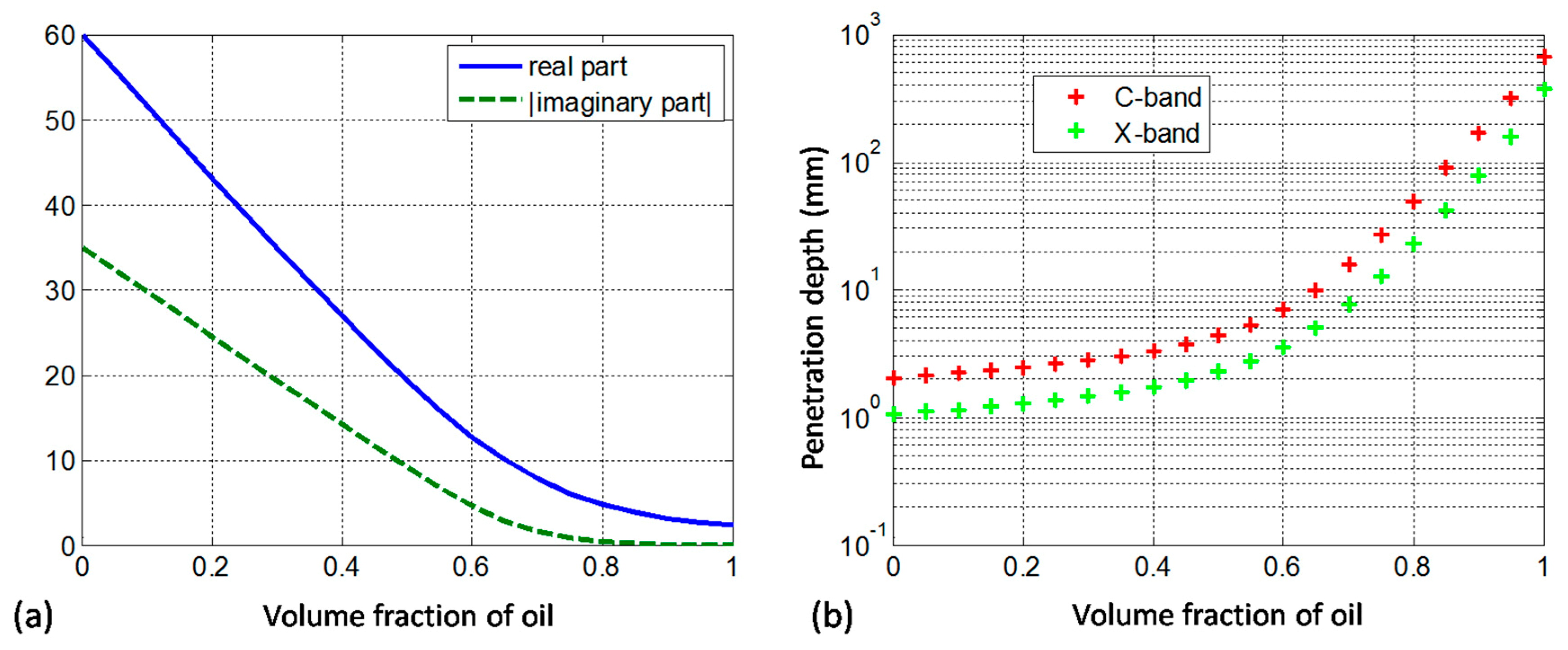
where , ranging from 0 to 1, is the oil volume content of the oil-water mixture. This effective dielectric constant behavior for a C-band case is plotted versus in Figure A1a, which demonstrates its strong nonlinear dependence on .
Figure A1.
(a) Effective dielectric constant of an oil-in-water emulsion vs. increasing volume fraction of oil (for C-band), (b) Penetration depth as a function of volume fraction of oil for C- and X-bands.
Figure A1.
(a) Effective dielectric constant of an oil-in-water emulsion vs. increasing volume fraction of oil (for C-band), (b) Penetration depth as a function of volume fraction of oil for C- and X-bands.

To assess the oil film influence on the reflectivity and polarization coefficients, the film thickness must be compared to the radio wave penetration depth (skin depth) . The latter is defined as the depth where the power of the propagating electric field is attenuated by a factor of 1/e and is calculated as [58]:
where denotes the imaginary part. The penetration depth depends strongly on the oil volume content (Figure A1b) and varies in a wide range of values. For clean water, is 2 and 1 mm for C- and X-bands, respectively; but for 100%, is several orders greater, 670 and 375 mm, respectively. For 20%–40%, typical for the oil-in-water emulsions [45], is 2.8 and 1.4 mm for C- and X-band, respectively, which is close to the values for clean water.
In the literature, considering the effects of the mineral oil dielectric constant on the reflection coefficients, different opinions have been expressed about these effects. Franceschetti et al. [61] studied the effect of a 1 mm thick mineral oil film (100%) on the sea surface reflection coefficients. This film was shown, for C-band and incidence angles less than 70°, to have a negligible effect on the reflection coefficients. Conversely, Minchew et al. [57], for the Deepwater Horizon case, used L-band with the corresponding penetration depth for clean water about 7–9 mm, and showed that the reflection coefficients became sensitive to the dielectric constant. This was a case of a radio thick slick since, according to Minchew et al. [57], a thick part of the upper layer of the ocean surface was likely a mixture of water and oil. Angelliaume et al. [28], observing oil-in-water emulsions in L-band, also concluded that the mineral oil dielectric constant impacted . This should occur in the case of a sufficiently thick emulsion film. Ideally, to obtain unambiguous conclusions in each case, it is necessary to have independent control of the film thickness.
Considering the oil-in-water emulsions used in 2011 and 2012 experiments, having a of 31%–42% (meaning water content of 58%–69%) and taking the conclusion from the experimental oil spill exercises and oil thickness assessment (Section 2) that most of the slick area likely consists of the film less than 0.1 mm thick and only a tiny part of the slick has a thickness greater than 1 mm, this thickness is about 30 times less than the penetration depth for C-band and about 15 times less for X-band. Therefore, the effect of the dielectric constant on the reflection coefficients should be small for most of the slick area (perhaps ~98% according to studies cited in Section 2). The rest of the slick area may be 1–9 mm thick, which is equal to or greater than for C- and X-bands; therefore, an impact of on the reflectivity and polarization coefficients should be significant for a tiny part of the slick area only.
References
- Espedal, H.A.; Johannessen, O.M. Detection of oil spills near offshore installations using Synthetic Aperture Radar (SAR). Int. J. Remote Sens. 2000, 21, 2141–2144. [Google Scholar] [CrossRef]
- Topouzelis, K.; Karathanassi, V.; Pavlakis, P.; Rokos, D. Detection and discrimination between oil spills and look-alike phenomena through neural networks. ISPRS J. Photogramm Remote Sens. 2007, 62, 264–270. [Google Scholar] [CrossRef]
- Alpers, W.; Holt, B.; Zeng, K. Oil spill detection by imaging radars: Challenges and pitfalls. Remote Sens. Environ. 2017, 201, 133–147. [Google Scholar] [CrossRef]
- Fingas, M.; Brown, C.E. A review of oil spill remote sensing. Sensors 2018, 18, 91. [Google Scholar] [CrossRef] [PubMed] [Green Version]
- Carpenter, A. Maritime Safety Agency CleanSeaNet activities oil pollution in the North Sea. In Oil Pollution in the North Sea; Carpenter, A., Ed.; Springer: Berlin/Heidelberg, Germany, 2015; pp. 33–47. ISBN 978-3-319-23901-9. [Google Scholar]
- Journel, M. CleanSeaNet. Unit C3. Satellite Based Monitoring Services. In 17ème Journée D’information Du Cedre: La Détection Des Pollutions Accidentelles Et Des Rejets Illicites; Cedre: Paris, France, 2012; Available online: https://wwz.cedre.fr/content/download/1229/10370/file/7-ensa-journel-fr.pdf (accessed on 24 March 2020).
- Solberg, A.H.S. Remote sensing of ocean oil-spill pollution. Proc. IEEE 2012, 100, 2931–2945. [Google Scholar] [CrossRef]
- Skrunes, S.; Brekke, C.; Eltoft, T. Characterization of marine surface slicks by radarsat-2 multipolarization features. IEEE Trans. Geosci. Remote Sens. 2014, 52, 5302–5319. [Google Scholar] [CrossRef] [Green Version]
- Migliaccio, M.; Nunziata, F.; Gambardella, A. On the co-polarized phase difference for oil spill observation. Int. J. Remote Sens. 2009, 30, 1587–1602. [Google Scholar] [CrossRef]
- Buono, A.; Nunziata, F.; de Macedo, C.R.; Velotto, D.; Migliaccio, M. A sensitivity analysis of the standard deviation of the copolarized phase difference for sea oil slick observation. IEEE Trans. Geosci. Remote Sens. 2018, 57, 2022–2030. [Google Scholar] [CrossRef]
- Migliaccio, M.; Nunziata, F.; Buono, A. SAR polarimetry for sea oil slick observation. Int. J. Remote Sens. 2015, 36, 3243–3273. [Google Scholar] [CrossRef] [Green Version]
- Hwang, P.A.; Perrie, W.; Zhang, B. Cross-polarization radar backscattering from the ocean surface and its dependence on wind velocity. IEEE Geosci. Remote Sens. Lett. 2014, 11, 2188–2192. [Google Scholar] [CrossRef]
- Hwang, P.A.; Stoffelen, A.; Zadelhoff, G.J.; Perrie, W.; Zhang, B.; Li, H.; Shen, H. Cross-polarization geophysical model function for C-band radar backscattering from the ocean surface and wind speed retrieval. J. Geophys. Res. Ocean. 2015, 120, 893–909. [Google Scholar] [CrossRef]
- Angelliaume, S.; Dubois-Fernandez, P.C.; Jones, C.E.; Holt, B.; Minchew, B.; Amri, E.; Miegebielle, V. SAR imagery for detecting sea surface slicks: Performance assessment of polarization-dependent parameters. IEEE Trans. Geosci. Remote Sens. 2018, 56, 4237–4257. [Google Scholar] [CrossRef] [Green Version]
- Montuori, A.; Nunziata, F.; Migliaccio, M.; Sobieski, P. X-band two-scale sea surface scattering model to predict the contrast due to an oil slick. IEEE J. Sel. Top. Appl. Earth Obs. Remote Sens. 2016, 9, 4970–4978. [Google Scholar] [CrossRef]
- Radarsat-2 Product Description, RN-SP-52-1238, Issue 1/14; MDA Ltd.: Richmond, BC, Canada, 2018.
- TerraSAR-X Image Product Guide, Basic and Enhanced Radar Satellite Imagery, Issue 2.0; Airbus Defense and Space: Ottobrunn, Germany, 2014.
- Del Frate, F.; Petrocchi, A.; Lichtenegger, J.; Calabresi, G. Neural networks for oil spill detection using ERS-SAR data. IEEE Trans. Geosci. Remote Sens. 2000, 38, 2282–2287. [Google Scholar] [CrossRef] [Green Version]
- Garcia-Pineda, O.; MacDonald, I.R.; Li, X.; Jackson, C.R.; Pichel, W.G. Oil spill mapping and measurement in the Gulf of Mexico with textural classifier neural network algorithm (TCNNA). IEEE IEEE J. Sel. Top. Appl. Earth Obs. Remote Sens. 2013, 6, 2517–2525. [Google Scholar] [CrossRef]
- Staples, G. Oil slick discrimination using RADARSAT-2 quad polarized data. In Proceedings of the Geoscience and Remote Sens. Symposium (IGARSS), 2015 IEEE International, Milan, Italy, 26–31 July 2015. [Google Scholar]
- Skrunes, S.; Brekke, C.; Eltoft, T.; Kudryavtsev, V. Comparing near coincident C- and X-band SAR acquisitions of marine oil spills. IEEE Trans. Geosci. Remote Sens. 2015, 53, 1958–1975. [Google Scholar] [CrossRef]
- Gade, M.; Alpers, W.; Hühnerfuss, H.; Lange, P.A. Wind wave tank measurements of wave damping and radar cross sections in the presence of monomolecular surface films. J. Geophys. Res. Ocean. 1998, 103, 3167–3178. [Google Scholar] [CrossRef]
- Gade, M.; Alpers, W.; Hühnerfuss, H.; Masuko, H.; Kobayashi, T. Imaging of biogenic and anthropogenic ocean surface films by the multifrequency/multipolarization SIR-C/X-SAR. J. Geophys. Res. Ocean. 1998, 103, 18851–18866. [Google Scholar] [CrossRef]
- Wismann, V.; Gade, M.; Alpers, W.; Huhnerfuss, H. Radar signatures of marine mineral oil spills measured by an airborne multi–frequency radar. Int. J. Remote Sens. 1998, 19, 3607–3623. [Google Scholar] [CrossRef]
- Nunziata, F.; Sobieski, P.; Migliaccio, M. The two-scale BPM scattering model for sea biogenic slicks contrast. IEEE Trans. Geosci. Remote Sens. 2009, 47, 1949–1956. [Google Scholar] [CrossRef]
- Kudryavtsev, V.N.; Chapron, B.; Myasoedov, A.G.; Collard, F.; Johannessen, J.A. On Dual co-polarized SAR measurements of the ocean surface. IEEE Geosci. Remote Sens. Lett. 2013, 10, 761–765. [Google Scholar] [CrossRef]
- Hansen, M.W.; Kudryavtsev, V.; Chapron, B.; Brekke, C.; Johannessen, J.A. Wave breaking in slicks: Impacts on C-band quad-polarized SAR measurements. IEEE J. Sel. Top. Appl. Earth Obs. Remote Sens. 2016, 9, 4929–4940. [Google Scholar] [CrossRef] [Green Version]
- Angelliaume, S.; Boisot, O.; Guérin, C.A. Dual-polarized L-band SAR imagery for temporal monitoring of marine oil slick concentration. Remote Sens. 2018, 10, 1012. [Google Scholar] [CrossRef] [Green Version]
- Nunziata, F.; de Macedo, C.R.; Buono, A.; Velotto, D.; Migliaccio, M. On the analysis of a time series of X–band TerraSAR–X SAR imagery over oil seepages. Int. J. Remote Sens. 2019, 40, 3623–3646. [Google Scholar] [CrossRef]
- Li, H.; Perrie, W.; Wu, J. Retrieval of oil–water mixture ratio at ocean surface using compact polarimetry synthetic aperture radar. Remote Sens. 2019, 11, 816. [Google Scholar] [CrossRef] [Green Version]
- Valenzuela, G.R. Theories for the interaction of electromagnetic and ocean waves—A review. Bound. Layer Meteorol. 1978, 13, 61–85. [Google Scholar] [CrossRef]
- Guérin, C.-A.; Soriano, G.; Chapron, B. The weighted curvature approximation in scattering from sea. surfaces. Waves Random Complex Media 2010, 20, 364–384. [Google Scholar] [CrossRef]
- Elfouhaily, T.; Guérin, C.-A. A critical survey of approximate scattering wave theories from random rough surfaces. Waves Random Media 2004, 14, R1–R40. [Google Scholar] [CrossRef]
- Kudryavtsev, V.N.; Hauser, D.; Caudal, G.; Chapron, B. A semiempirical model of the normalized radar cross-section of the sea surface: 1. Background model. J. Geophys. Res. 2003, 108. [Google Scholar] [CrossRef] [Green Version]
- Ivonin, D.V.; Skrunes, S.; Brekke, C.; Ivanov, A.Y. Interpreting sea surface slicks on the basis of the normalized radar cross-section model using Radarsat-2 copolarization dual-channel SAR images. Geophys. Res. Lett. 2016, 43, 2748–2757. [Google Scholar] [CrossRef] [Green Version]
- Ivonin, D.V.; Ivanov, A.Y. On classification of sea surface oil films using TerraSAR-X satellite polarization data. Oceanology 2017, 57, 738–750. [Google Scholar] [CrossRef]
- Skrunes, S.; Brekke, C.; Doulgeris, A.P. Characterization of low-backscatter ocean features in dual-copolarization SAR using log-cumulants. IEEE Geosci. Remote Sens. 2015, 12, 836–840. [Google Scholar] [CrossRef]
- Banner, M.L.; Fooks, E.H. On the microwave reflectivity of small-scale breaking water waves. Proc. R. Soc. Lond. Ser. A. Math. Phys. Sci. 1985, 399, 93–109. [Google Scholar]
- Ericson, E.A.; Lyzenga, D.R.; Walker, D.T. Radar backscattering from stationary breaking waves. J. Geophys. Res. 1999, 104, 29679–29695. [Google Scholar] [CrossRef]
- Phillips, O.M. Radar returns from the sea surface Bragg scattering and breaking waves. J. Phys. Oceanogr. 1988, 18, 1063–1074. [Google Scholar] [CrossRef]
- Caulliez, G.; Guérin, C.A. Higher-order statistical analysis of short wind wave fields. J. Geophys. Res. 2012, 117. [Google Scholar] [CrossRef] [Green Version]
- Caulliez, G. Dissipation regimes for short wind waves. J. Geophys. Res. Ocean. 2013, 118, 672–684. [Google Scholar] [CrossRef]
- Jones, C.E.; Dagestad, K.-F.; Breivik, Ø.; Holt, B.; Röhrs, J.; Christensen, K.H.; Espeseth, M.; Brekke, C.; Skrunes, S. Measurement and modeling of oil slick transport. J. Geophys. Res. Ocean. 2016, 121, 7759–7775. [Google Scholar] [CrossRef]
- Moldestad, M.Ø.; Schrader, T. ESSO BJR9: Ringhorne, Forseti og Balder; Egenskaper og Forvitring på Sjøen Relatert til Beredskap; Technical Report STF66 A01137; SINTEF: Trondheim, Norway, 2002; p. 93. Available online: https://docplayer.me/20723266-Esso-bjr9-ringhorne-forseti-balder-crude-oil-revidert-rapport-forfatter-e-oppdragsgiver-e.html (accessed on 24 March 2020)ISBN 82-14-02296-7.
- Daling, P.S.; Moldestad, M.Ø.; Johansen, Ø.; Lewis, A.; Rødal, J. Norwegian testing of emulsion properties at sea––The importance of oil type and release conditions. Spill Sci. Technol. Bull. 2003, 8, 123–136. [Google Scholar] [CrossRef]
- Svejkovsky, J.; Hess, M.; Muskat, J.; Nedwed, T.J.; McCall, J.; Garcia, O. Characterization of surface oil thickness distribution patterns observed during the deepwater horizon (MC-252) oil spill with aerial and satellite remote sensing. Mar. Pollut. Bull. 2016, 110, 162–176. [Google Scholar] [CrossRef]
- Svejkovsky, J.; Muskat, J. Development of a portable multispectral aerial sensor for real-time oil spill thickness mapping in coastal and offshore waters. In Final Report for U. S. Minerals Management Service Contract M07PC13205; U. S. Minerals Management Service: Washington, DC, USA, 2009; p. 33. [Google Scholar]
- Galt, J.A.; Overstreet, R. Development of spreading algorithms for the ROC. In Response Options Calculator (ROC); Technical Note; Genwest Systems: Edmonds, WA, USA, 2009; Available online: https://www.genwest.com/resources/tech/Development-of-Spreading-Algorithms-for-the-ROC.pdf (accessed on 24 March 2020).
- Tansel, B.; Kumar, V. Effect of sea conditions on emulsification profile of oils in coastal waters after major spills. In World Environmental and Water Resources Congress, May 22–26, 2011; American Society of Civil Engineers: Reston, VA, USA, 2011; pp. 1826–1829. [Google Scholar]
- Bonn Agreement. Bonn Agreement Aerial Operations Handbook. 2016, p. 123. Available online: https://www.bonnagreement.org/site/assets/files/1081/aerial_operations_handbook.pdf (accessed on 24 March 2020).
- Barrick, D.E. Accuracy of parameter extraction from sample-averaged sea-echo Doppler spectra. IEEE Trans. Antennas Propag. 1980, 28, 1–11. [Google Scholar] [CrossRef]
- Ivonin, D.; Ivanov, A.Y. Dependence of the noise level estimates supplied with TerraSAR-X data on the used preprocessor version. Sovrem. Probl. Distantsionnogo Zondirovaniya Zemli Kosm. 2019, 16, 45–50. [Google Scholar] [CrossRef]
- COSMO-SkyMed Mission and Products Description. Italian Space Agency. Doc. N.: ASI-CSM-PMG-NT-001. 8 July 2019, p. 151. Available online: https://www.asi.it/wp-content/uploads/2019/08/COSMO-SkyMed-Mission-and-Products-Description_rev3-2.pdf (accessed on 24 March 2020).
- Nunziata, F.; Buono, A.; Migliaccio, M. COSMO-SkyMed synthetic aperture radar data to observe the deepwater horizon oil spill. Sustainability 2018, 10, 3599. [Google Scholar] [CrossRef] [Green Version]
- Wright, J. Backscattering from capillary waves with application to sea clutter. IEEE Trans. Antennas Propag. 1966, 14, 749–754. [Google Scholar] [CrossRef]
- Hwang, P.A.; Zhang, B.; Toporkov, J.V.; Perrie, W. Comparison of composite Bragg theory and quad-polarization radar backscatter from Radarsat-2: With applications to wave breaking and high wind retrieval. J. Geophys. Res. Ocean. 2010. [Google Scholar] [CrossRef] [Green Version]
- Minchew, B.; Jones, C.E.; Holt, B. Polarimetric analysis of backscatter from the deepwater horizon oil spill using L-band synthetic aperture radar. IEEE Trans. Geosci. Remote Sens. 2012, 50, 3812–3830. [Google Scholar] [CrossRef]
- Ulaby, F.T.; Moore, R.K.; Fung, A.K. Microwave Remote Sens.: Active and Passive; Radar Remote Sens. and Surface Scattering and Emission Theory (vol. II); Artech House: Norwood, MA, USA, 1986; ISBN 0-89006-191-2. [Google Scholar]
- Brekke, C.; Holt, B.; Jones, C.; Skrunes, S. Discrimination of oil spills from look-alikes in the marginal ice zone by synthetic aperture radar. Remote Sens. Environ. 2014, 145, 1–14. [Google Scholar] [CrossRef]
- Sihvola, A. Electromagnetic Mixing Formulas and Applications; Institution of Electrical Engineers: London, UK, 1999. [Google Scholar]
- Franceschetti, G.; Iodice, A.; Riccio, D.; Ruello, G.; Siviero, R. SAR raw signal simulation of oil slicks in ocean environments. IEEE Trans. Geosci. Remote Sens. 2002, 40, 1935–1949. [Google Scholar] [CrossRef]
Figure 1.
(a) Subscene of the RSb image(see Table 1), VV (vertical transmit and vertical receive) polarization, acquired June 8, 2011 17:27 UTC (shaded bar in dB); (b) subscene near the RSb_P slick (see Table 2), the blue rectangle outlines clean water pixels, whose mean is taken as a clean water reference level, red points indicate pixels having a signal level less than 0.4 of the water signal, and (c) the same for the RSb_E slick (see Table 2). Axes are pixel numbers; each pixel has a size of 8 × 8 of the original pixel size (Table 1); grey half-tones are the same for each of the subscenes.

Figure 2.
(a) Subscene of the RSd VV image (see Table 1). (b) Histogram of for pixels in the RSd_E4 processing area. (c) for slicks of the RSd image. (d) Subscene of the RSb VV image (see Table 1). (e) for the RSd_E4 processing area; the color indicates the number of points on a base 10 logarithmic scale. (f) for the corresponding processed slicks on the RSb image.

Figure 3.
(a) Subscene of the RSc VV image (see Table 1). (b) Cross-sections of , , and through the slick RSc_E2 (for 300 m × 300 m smoothing). and refer to 8 × 8 multi-looking case. (c) Corresponding cross-sections of and . (d) for the RSc_E2. (e) Subscene of the TSc VV image (see Table 1). (f) Cross-sections of , , and and (g) cross-sections of , , and through the slick TSc_E2. (h) for the slicks TSc_E1, TSc_E2, and TSc_E3.

Figure 4.
(a) Subscene of the TSa VV image (see Table 1). (b) Cross-sections of , , and through the slick. (c) Corresponding cross-sections of and . (d) for the slick TSa_E. (e) Subscene of the RSa VV image (see Table 1). (f) Cross-sections of , , and through the RSa_E slick, whose position is indicated by the white dashed line in (e). (g) Corresponding cross-sections of and through the RSa_E slick. (h) for the slicks RSa_E and RSa_P.

Figure 5.
Slick resonant and non-resonant signal damping and (error bar) vs. the Bragg wavenumber for oil spills visible on RS and TS images. The dotted line indicates the most likely position for mineral oil . The dashed lines indicate upper and lower boundaries of mineral oil .
Figure 5.
Slick resonant and non-resonant signal damping and (error bar) vs. the Bragg wavenumber for oil spills visible on RS and TS images. The dotted line indicates the most likely position for mineral oil . The dashed lines indicate upper and lower boundaries of mineral oil .

Figure 6.
(a) Histogram for the number of slicks detected with appropriate confidence level to belong the right slick type; (b) the confidence level of the detection of the right slick type vs. .
Figure 6.
(a) Histogram for the number of slicks detected with appropriate confidence level to belong the right slick type; (b) the confidence level of the detection of the right slick type vs. .

Table 1.
Information on the collected synthetic aperture radar (SAR) images.
| Date | Time, UTC | Scene Coding | Pass Direction | Incidence Angle | SNRslick a | Image Pixel Spacing b, (Rg × Az), m | Measured Wind c, m/s | Oil Slick Type |
|---|---|---|---|---|---|---|---|---|
| June 8, 2011 morning | 05:59 06:23 | RSa TSa | Desc. Desc. | 46.1°–47.3° 27.3°–29.0° | >−3 dB >8 dB | 6.48 × 4.70 1.88 × 2.35 | 1.6–3.3 ESE | emulsion, plant oil, emulsion |
| June 8, 2011 evening | 17:27 - | RSb - | Asc. | 34.5°–36.1° | >5 dB | 8.17 × 4.81 | 1.6–3.3 Var. d (E) | ecrude oil, emulsion, plant oil |
| June 15, 2012 evening | 17:48 17:28 | RSc TSc | Asc. Asc. | 48.3°–49.5° 40.9°–42.1° | >2 dB >0 dB | 6.26 × 5.11 1.34 × 2.25 | 6(3) (NE) 5–6 (3.5) (NE) | emulsion n.2 emulsions n.1,2,3 |
| June 5, 2012 morning | 06:20 - | RSb - | Desc. | 30.1°–30.8° | >7 dB | 9.12 × 5.59 | 4 NE | emulsions n.4,5,6 plant oil |
a Meaning the SNR in the slick for the HH channel. b The range resolution is obtained taking into account the incidence angle. c Wind was measured at the ships participating in the exercises, whereas the measurements within parentheses were acquired at the production platform located closest to the exercise site (the Heimdal platform, 59°34′27.30″N 2°13′22.60″E). d ’Var.’ denotes variable wind direction.
Table 2.
Properties of the releases and estimated mean film thicknesses.
| Slick | Substance | Water Content a | Age, h | Volume of Release, m3 | SAR slick Area Estimate b, km2 | Mean Film Thickness Based on the SAR Slick Area d, µm |
|---|---|---|---|---|---|---|
| RSa_P | Radiagreen EBO | None | 2 | 0.4 | 0.11 | 3.5 |
| RSb_P | ″ | ″ | 13 | ″ | 1.58 | 0.3 |
| RSd_P | ″ | ″ | 14 | ″ | 1.16 | 0.3 |
| RSa_E | Emulsion of Oseberg blend | 69% | 18 | 20 | 2.35 | 9 |
| TSa_E | ″ | ″ | ″ | ″ | 2.07 | 10 |
| RSb_E | ″ | ″ | 29 | ″ | 0.87 | 23 |
| RSb_C | Balder crude oil | None | 9 | 30 | 4.84 | 6 |
| TSc_E1 | Emulsion of Oseberg blend | 58% | 28–29 | 17 | 0.77 | 22 |
| RSc_E2 | ″ | ″ | 25 | 10 | 0.64 | 16 |
| TSc_E2 | ″ | ″ | ″ | ″ | 0.84 | 12 |
| TSc_E3 | ″ | ″ | 12 | 25 | 1.57 | 16 |
| RSd_E4 | ″ | ″ | 22 | - c | 4.17 | - |
| RSd_E5 | ″ | ″ | 17 | - c | 3.37 | - |
| RSd_E6 | ″ | ″ | 14 | - c | 10.25 | - |
a Initial. b Calculated using corresponding dark area on SAR scenes. c Unknown exact value. d This value is very uncertain since some of the releases were very old and the volume was changing.
Table 3.
Parameters of oil slicks, SAR images and corresponding calculated parameters.
| Oil Film Type (Coding) | Incidence Angle a | NESZ, dB | Signal in Slick b, / | Signal in slick b, / | RND a (Mean ± std) | Confidence Level to Be Mineral Oil a,c, % | Confidence Level to Be Plant Oil a,c, % | ||
|---|---|---|---|---|---|---|---|---|---|
| plant oil (rsb_p) | 35.2° 35.3° | −35.1 | −22.3/−23.7 | −26.4/−24.5 | −8.1/−5.1 | 11.4/17.1 11.4/16.7 | 0.782 ± 0.029 0.773 ± 0.046 | 18 15 | 82 85 |
| emulsion (RSb_E) | 35.6° 35.4° | −34.9 | −25.1/−26.8 | −28.6/−27.8 | −8.9/−6.8 | 8.1/15.4 9.9/16.4 | 0.888 ± 0.048 0.854 ± 0.026 | 83 84 | 4 16 |
| crude oil (RSb_C) | 35.9° 36.0° | −34.1 | −28.0/−29.3 | −32.3/−30.0 | −12.5/−8.6 | 4.8/14.2 3.7/13.7 | 0.882 ± 0.024 0.881 ± 0.024 | 100 100 | 0 0 |
| plant oil (RSd_P) | 31.5° | −35.2 | −23.1/−24.7 | −26.1/−26.1 | −6.6/−4.9 | 10.5/15.9 | 0.759 ± 0.032 | 0 | 100 |
| emulsion 4 (RSd_ E4) | 31.1° | −35.5 | −25.3/−26.6 | −29.3/−27.6 | −11.1/−8.5 | 8.9/18.1 | 0.892 ± 0.024 | 100 | 0 |
| emulsion 5 (RSd_E5) | 31.1° | −35.5 | −26.8/−28.3 | −30.1/−29.5 | −11.4/−10.1 | 7.2/17.7 | 0.930 ± 0.024 | 100 | 0 |
| emulsion 6 (RSd_E6) | 31.2° | −35.5 | −25.3/−26.7 | −28.7/−27.9 | −9.5/−8.2 | 8.8/17.4 | 0.909 ± 0.018 | 100 | 0 |
| emulsion 2 (RSc_E2) | 49.5° | −31.1 | −24.5/−28.8 | −26.1/−29.7 | −5.9/−4.2 | 2.3/6.9 | 0.802 ± 0.047 | 68 | 32 |
| emulsion 1 (TSc_E1) | 41.3° | −23.2 | −20.4/−22.6 | −23.3/−23.5 | −5.4/−3.1 | 0.5/4.1 | 0.753 ± 0.032 | 88 | 0 |
| emulsion 2 (TSc_E2) | 41.5° | −23.3 | −21.5/−23.4 | −25.3/−24.0 | −7.0/−3.4 | −0.1/4.0 | 0.686 ± 0.032 | 80 | 20 |
| emulsion 3 (TSc_E3) | 41.7° | −23.0 | −21.8/−23.4 | −25.9/−23.9 | −8.4/−4.1 | −1.0/4.5 | 0.717 ± 0.037 | 81 | 19 |
| emulsion (RSa_E) | 46.6° | −32.8 | −30.1/−35.5 | −31.0/−37.6 | −7.9/−6.0 | −2.7/4.1 | 0.915 ± 0.063 | 55 | 0 |
| plant oil (RSa_P) | 47.0° | −32.6 | −25.0/−31.0 | −25.6/−33.4 | −3.0/−2.3 | 1.6/4.3 | 0.810 ± 0.048 | 65 | 35 |
| emulsion (TSa_E) | 28.2° | −26.6 | −18.2/−18.9 | −24.2/−19.5 | −7.8/−4.9 | 7.7/13.1 | 0.840 ± 0.023 | 87 | 0 |
a The first value is provided for the part of the slick marked by a solid line on the corresponding figures, the second is for the part marked by the dashed line. b For the chosen rectangle, the minimum was calculated using the 300 m × 300 m smoothed image. c The sum of the values within the last 2 columns in Table 3 is not 100% since sometimes there is a part of the RND distribution lying out the integration upper boundary. Therefore this part is excluded from the integration and the sum is less than 100%.
Table 4.
Estimated effects of various observation and weather condition parameters on the RND variations for mineral oils.
Table 4.
Estimated effects of various observation and weather condition parameters on the RND variations for mineral oils.
| Parameter | Tested Working Range | Preliminary Estimated Effect on the RND Trend |
|---|---|---|
| Frequency | C-band, X-band | <10% |
| Incidence angle | 28°–49° | <20% c |
| Wind speed | 2–6 m/s | <20% c |
| Wind direction | no | <20% c |
| Tilts of long waves | no | ? |
| Slick age | 9–29 h | <20% c |
| Minimal SNR a, water/slick b | 5 dB/−2 b dB | <20% c |
a For 70% confidence level to be inside the mineral oil zone. b At 300 m × 300 m multi-looking. c Sum of all these effects is ~20%, therefore each effect separately must give less than 20%.
© 2020 by the authors. Licensee MDPI, Basel, Switzerland. This article is an open access article distributed under the terms and conditions of the Creative Commons Attribution (CC BY) license (http://creativecommons.org/licenses/by/4.0/).
Share and Cite
MDPI and ACS Style
Ivonin, D.; Brekke, C.; Skrunes, S.; Ivanov, A.; Kozhelupova, N. Mineral Oil Slicks Identification Using Dual Co-polarized Radarsat-2 and TerraSAR-X SAR Imagery. Remote Sens. 2020, 12, 1061. https://doi.org/10.3390/rs12071061
AMA Style
Ivonin D, Brekke C, Skrunes S, Ivanov A, Kozhelupova N. Mineral Oil Slicks Identification Using Dual Co-polarized Radarsat-2 and TerraSAR-X SAR Imagery. Remote Sensing. 2020; 12(7):1061. https://doi.org/10.3390/rs12071061
Chicago/Turabian StyleIvonin, Dmitry, Camilla Brekke, Stine Skrunes, Andrei Ivanov, and Nataliya Kozhelupova. 2020. "Mineral Oil Slicks Identification Using Dual Co-polarized Radarsat-2 and TerraSAR-X SAR Imagery" Remote Sensing 12, no. 7: 1061. https://doi.org/10.3390/rs12071061
Note that from the first issue of 2016, this journal uses article numbers instead of page numbers. See further details here.