Hybrid Overlap Filter for LiDAR Point Clouds Using Free Software


1
GI-1934 TB-Biodiversity-LaboraTe, Department of Agroforestry Engineering and IBADER, University of Santiago de Compostela, ES-27001 Lugo, Spain
2
SIT-Sistema de Información Territorial, University of Santiago de Compostela, ES-27001 Lugo, Spain
*
Author to whom correspondence should be addressed.
†
These authors contributed equally to this work.
Remote Sens. 2020, 12(7), 1051; https://doi.org/10.3390/rs12071051
Submission received: 6 February 2020
/
Revised: 19 March 2020
/
Accepted: 22 March 2020
/
Published: 25 March 2020
(This article belongs to the Section Remote Sensing in Geology, Geomorphology and Hydrology)
Abstract
:Despite the large amounts of resources destined to developing filtering algorithms of LiDAR point clouds in order to obtain a Digital Terrain Model (DTM), the task remains a challenge. As a society advancing towards the democratization of information and collaborative processes, the researchers should not only focus on improving the efficacy of filters, but should also consider the users’ needs with a view toward improving the usability and accessibility of the filters in order to develop tools that will provide solutions to the challenges facing this field of study. In this work, we describe the Hybrid Overlap Filter (HyOF), a new filtering algorithm implemented in the free R software environment. The flow diagram of HyOF differs in the following ways from that of other filters developed to date: (1) the algorithm is formed by a combination of sequentially operating functions (i.e., the output of the first function provides the input of the second), which are capable of functioning independently and thus enabling integration of these functions with other filtering algorithms; (2) the variable penetrability is defined and used, along with slope and elevation, to identify ground points; (3) prior to selection of the seed points, the original point cloud is processed with the aim of removing points corresponding to buildings; and (4) a new method based on a moving window, with longitudinal overlap between windows and transverse overlap between passes, is used to select the seed points. Our hybrid filtering method is tested using 15 reference samples acquired by the International Society of Photogrammetry and Remote Sensing (ISPRS) and is evaluated in comparison with 33 existing filtering algorithms. The results show that our hybrid filtering method produces an average total error of 3.34% and an average Kappa coefficient of 92.62%. The proposed algorithm is one of the most accurate filters that has been tested with the ISPRS reference samples.
1. Introduction
In the last few decades, the static views of the environment, provided by conventional cartographic methods [1], have been substituted by digital mapping tools that enable construction of 3D models based on data with geographical content [2]. Although the development of these models was originally limited to a few users, the arrival of the Internet and the advances made in the field of informatics and computing have enabled the same data to be used to create maps that are available to millions of people. Thus, map users have progressed to being designers capable of sharing their view of the environment with the world. The way in which terrain is now represented is a good example of the advances made. At present, the great diversity of methods used to obtain georeferenced data, the volume of these data, and the wide spectrum of possible ways of obtaining information have shaken the foundations of terrain mapping. Although many techniques can be used to acquire topographical data (e.g., classic topographical methods, photogrammetry, interferometric InSAR), LiDAR technology is considered one of the standard methods for acquiring such data [3,4].
More than a decade ago, the work in [5] identified the limited efficiency of the post-processing LiDAR data as one of the challenges to be addressed by the commercial sector. This author reported that between 60% and 80% of the relevant resources are destined to the manual classification of data and the quality control. However, new and complex filtering algorithms have since been developed, supported by technological advances, free software, and the massive availability of data. Although private companies (and public bodies) are generally not transparent about the efficiency of these processes, refined manual processes of models and quality control continue to represent an important part of the workflow of commercial projects [6]. Despite the efforts made in this field, the scientific community considers that the problem has not been totally resolved, and the search for the perfect algorithm continues [7,8,9]. This is amply demonstrated by the continued production of filters over the years (Figure 1).
With the aim of responding to the new challenges regarding terrain mapping and to address the limitations of classic filtering strategies (Table 1), the current tendency is to integrate various filtering methods/processes to take advantage of the strengths of each, thus giving rise to so-called hybrid methods [10]. Most of these filters are developed from existing algorithms, which are modified to mitigate some of their limitations. The main type of modification is (a) to combine various methods or (b) to add a complementary process.
Regarding the first option (to combine various methods), some authors have combined morphological filters and different types of filters such as surface or interpolation [11,12,13], while others have combined segmentation and densification processes [14,15]. As an example of the latter, the work in [16] improved the hybrid method of [17] by combining the Progressive TINDensification (PTD) method of [18] with the segmentation method proposed by [19]. Thus, once the point cloud is segmented, the segments with a proportion of multiple returns greater than 50% are disregarded as being considered representative of vegetation. The ground segments are then gradually densified, and the unit of analysis changes from being a simple point to being a segment. This combination enables the number of seed points to be increased, particularly in urban zones, where the PTD method is strengthened by using a larger window size to avoid introducing commission errors due to the presence of large buildings. Although the method reduces the omission errors relative to the classic PTD method, the number of commission errors is greater, which the classic method had attempted to prevent.
Other authors have opted for the second method and included complementary processes in existing algorithms. The work in [22] introduced a decimation process for non-ground points posterior to the selection of seed points in the Sequential Iterative Dual-Filter (SIDF). This algorithm has only been tested in rural areas, and although it yielded better results than most algorithms considered in the study of [23], the high commission errors led to the total error in these zones being higher than that produced by other algorithms developed in the same period (e.g., [12] or [24]).
The methods developed by [24] represent another two examples of the versatility of hybrid methods. In the first of these, Segmentation Modeling and Surface Modeling (SMSM), segmentation is combined with a densification process. The second process is known as the Slope-based Statistical Algorithm (SSA). Both algorithms are preceded by decimation of the raw point cloud, with the aim of removing points representing vegetation, prior to selection of seed points. The decimation method assumes that vegetated zones produce multiple returns, in contrast to impermeable zones, which only produce a single return. This decimation method has proven to be highly effective for removing vegetation points, thus reducing the probability of introducing commission errors in the seed point cloud. This particularly applies to forest areas, where the size of the window could be reduced during the selection of the local lowest points by the use of this method to complement a classic densification algorithm. However, this advantage is not observed in urban areas. Although commission errors have a negative influence on the quality of the final model, the magnitude of the errors is much greater when they are produced in urban zones, as it is more likely that the incorrect classification of the points will occur in built-up areas than in vegetated areas [25]. Therefore, in urban zones, it will not be possible to reduce the selection window size of the local lowest points without greatly increasing the number of commission errors. These types of methods provide novel, versatile, and effective solutions to the problem of identifying ground points. However, methods that use complementary processes basically focus on improving the results in vegetated zones, without effectively resolving the problem of the large numbers of commission errors in urban zones.
Finally, identifying the filter that best adapts to the specific needs of the user is not a simple task, as it assumes a good level of knowledge about the different filters. In many cases, such knowledge is difficult to acquire due to the lack of usability (ease of use - according to [26], usability is the degree of efficacy, efficiency, and satisfaction with which the user can achieve the specific objectives desired, within the context of the particular use. In the present case, we refer to usability only in the sense of the subjective attribute: satisfaction [27]) and accessibility (possibility of access-in computer science, the term “accessibility” refers to the design of products to be usable by people with disabilities. However, in this paper, this term refers only to the “free access” and intends to represent the opposite of what the commercial software depicts). These obstacles are exacerbated by the fact that many of the filtering details are jealously guarded by their creators [17] and are not published, while those included in commercial software act like black boxes that operate on data. In response to this situation, in this work, we present the Hybrid Overlap Filter (HyOF), a new filtering algorithm implemented in the free R software environment [28]. In addition to being aimed at reducing the number of commission errors associated with the selection of the seed points in urban areas, the algorithm also aims to respond to some of the actual needs of the users. The algorithm follows the overall scheme of most densification filters developed to date, but HyOF also incorporates a decimation process [20], making it a hybrid method.
2. Methodology
The HyOF filter is a hybrid algorithm that uses the flow diagram of densification filters as a reference point. However, it differs in four ways relative to these filters. The first difference is that the HyOF filter is formed by a combination of sequentially operating functions (i.e., the output of the first function is the input of the second), which are capable of functioning independently and can therefore be included in other filters, as demonstrated in [20]. Moreover, in addition to using the variables’ slope and elevation to identify the Local Lowest Points (LLP), HyOF defines and uses the variable penetrability. The third difference is that as a first step prior to selecting the LLP, in a similar approach to that used by [24], the original point cloud is subjected to a decimation process aimed at detecting and removing (under some circumstances) the non-ground points corresponding to buildings and vegetation. This step makes it possible to reduce the window size for selecting the seed points, thus increasing the number of points selected without increasing the commission errors. This enables a better definition of the ramps and inner courtyards of buildings and prevents the erroneous selection of points corresponding to buildings as LLP. Finally, the remaining difference is based on the assumption that the locally selected points with minimal elevation are sufficient to define the main terrain characteristics and to generate a first reference surface. Thus, we place particular emphasis on attempting to improve the process of selecting the LLP, and a method of selecting LLP that uses a moving window with longitudinal and transverse displacement is developed. HyOF is implemented in the free R software environment [28] in an attempt to address the challenge of the usability and accessibility of the LiDAR data processing methods. The filtering parameters, the functions, and the flowchart of our hybrid filter are described below.
2.1. The Filtering Parameters
The parameters of our hybrid filter can be grouped into three categories: fixed (remaining constant in all study areas); variable (set by the user); and automatic (automatically set during the filtering process). Table 2 includes a brief description of all parameters used in our hybrid filter.
2.2. Description of Functions Included in HyOF
2.2.1. Selection of Seed Points: OWM Function
The Local Minimum Method (LMM) is one of the most popular methods for selecting seed points due to its simplicity and efficiency. The main limitation of this method is the selection of the window size, which should be large enough to minimize the influence of the non-ground points and small enough to conserve the characteristics of the relief [29]. In areas where buildings coexist with complex orography, particular attention should be given to the value of this parameter. In this case, the window size used to minimize the influence of the non-ground points will be too large to preserve the details of the relief. In complex forest zones (e.g., surfaces with different densities of vegetation on hillsides), the window size does not need to be as large as in the previous case; however, it will also not be small enough to produce a detailed estimate of the terrain surface, as densely vegetated zones have negative effects similar to those of the buildings in the previous case. The Overlap Window Method (OWM) is developed with the aim of minimizing these limitations. This method is defined by five parameters: input LiDAR data (P), window size for selecting the local lowest points (w), the size of the mesh for identification of zones without local lowest points (W), longitudinal overlap (O), and transverse overlap (O) between windows (expressed as a decimal). The flow diagram for this function are outlined in Figure 2.
First, the geographical scope of extraction of the local lowest points is defined using the maximum and minimum values of the x-coordinate and y-coordinate of the point cloud (x, x, y, y). The area is extended by applying an exterior buffer of magnitude w · O on the x-axis and w · O on the y-axis, to analyze the edge points as many times as the rest of points. A moving window of size w is displaced from the Bottom Left Corner (BLC) following the direction of the x-axis with an overlap between consecutive windows of magnitude w · O. At the end of the first pass, the window w returns to the extreme left and begins a new pass, whose origin is displaced w · O in the y-axis relative to the first pass. The process is repeated until the window w reaches the Top Right Corner (TRC) (Figure 2a). In each position of the window, the lowest point is selected, giving rise to a set of local lowest points. As a result of the overlap between windows, the same point may be selected more than once. Logically, those points selected various times are more likely to be ground points than those points selected once. Thus, the points selected more than once are finally those considered seed points (Figure 2b). In high-slope zones, it is unlikely that the same point will be identified as a local lowest point more than once, and the resulting seed-point cloud will have some zones without points. In order to minimize the lack of detail in these zones, a grid of square cells of size W is fitted to the geographical scope (Figure 2c). For those cells without points, the lowest point is selected from the original point cloud (Figure 2d) and is added to the final seed-point cloud (Figure 2e).
2.2.2. Calculation of Penetrability: PNT Function
The penetrability (PNT) is defined as the ratio between the number of ground points and the number of total points in each cell. The PNT function is developed in order to calculate this variable. Figure 3 shows the pseudo-code of the PNT function. This function is defined by four parameters: input LiDAR data (P); reference terrain surface (); cell size (W); and the value of the residual from which a point is considered a non-ground point (). The difference in elevation between LiDAR points and the reference terrain surface is first calculated (). A point is considered a ground point and encoded as G, if < . A grid of square cells of size W, whose extension coincides with the zone for which data are available, is created. For each cell, the value resulting from dividing the number of points coded as G by the total number of points is calculated. Empty cells are represented as Not Available (NA). The result of the PNT function is (raster format).
2.2.3. Decimation of the Point Cloud: DecHPoints Function
The filters that include a selection process of local lowest points must adapt the size of the selection window according to the characteristics of the study area, with the aim of preventing commission errors due to the presence of objects. Smaller windows lead to the selection of more local lowest points and, in urban zones with large buildings, to a greater risk of erroneous selection of non-ground points as ground points. Logically, the selection process of the local lowest points will be more effective when the number of building points in the original point cloud is minimal. Thus, in urban areas, it would be possible to use a window of a similar size to that used in forest zones and thus reduce the risk of erroneously including non-ground points in the cloud of local lowest points.
Following the studies of [22,24], we developed and used the Decimation of Highest Points function (DecHPoints) to produce a decimated point cloud (P) by detecting and deleting (under some circumstances) the highest points in a local environment from the point cloud. The underlying principle that this function applies to detect and remove non-ground points from the point cloud is that the elevations of these points are maximal in local environments. The DecHPoints function is defined by six parameters: input LiDAR data (P); the maximum size of the area without ground points (usually identified from the shortest side of the largest building in the study area (c); surface penetrability (); minimum and maximum slope thresholds (S and S); and allowed maximum residual (). The pseudo-code of DecHPoints is shown in Figure 4.
First, the mean weighted density is calculated from LiDAR data (D). Then, the point cloud is decimated at two Levels (L), and the same operations are used at both levels to produce the decimated point cloud (P). On the other hand, the size of the search window (W), used to identify the highest points, and the window of analysis (W), used to analyze and to decide whether or not those points are ground points, are defined on the basis of parameter c. At the first level (L = 1), the size of W (H) is c. However, as the window used to search for the highest points (W) should include ground points and non-ground points, a coefficient of 1.5 is applied to the size of W in order to establish the size of W (1.5 · H). The coefficient is established by trial and error and by checking the quality of results. In addition, the theoretical number of points that should be included in a window W is calculated as by multiplying D and (1.5 · H).
Secondly, the geographical scope is defined by the data zone plus an exterior buffer of 0.5 times the size of W. This exterior buffer is used to analyze the edge points as many times as the rest of points (prevent the edge effect). Then, W is moved from the BLC to the TRC, and a longitudinal and transverse overlap between windows equal to 50% is applied (O = 0.5). In each position, all points that are included within the window W are selected (P). If the number of P () is lower than 10% of , the decimation process is not required. P points are then selected and became part of the decimated point cloud (P). New points are selected by moving the window W from left to right by O times the size of W. Conversely, if NP ≥ 0.1 · , the highest point (p) in P is selected. In order to decide whether or not p is a ground point, a local area defined by W and centered in p is considered. In this area, points neighboring p are selected (P), and the lowest point is identified (p). Finally, the slope between p and p is calculated (Sl).
Three situations are then considered: (1) If the elevations of p and p are the same or the slope between p and p is less than S, P points (including p) are considered ground points and therefore added to P. The window W is then moved one position; the new points are selected; and the number of P is re-evaluated. (2) If the slope between p and p is greater than S, then p is removed from P; a new highest point (in P) is selected; and the previous steps are repeated to check whether or not p is a ground point. (3) Finally, if S < Sl < S, no decision could be reached on the basis of the slope and the difference in elevation relative to p, and therefore, a reference surface () (This surface is created by interpolating a set of lowest points selected from P in the cells of whose penetrability is more than zero. The thin plate spline method, recognized as an effective method for interpolating spatial data [29,30], is used to generate the .) is taken into account to calculate the residual from p (p = (x,y,z,)). Then, if is greater than , p is removed from P, and a new highest point is selected. Otherwise, P points (including p) are considered ground points and added to P. The window W is then moved one position, the new points are selected (P) and the number of P re-evaluated.
At the second level, the above process is repeated considering the refined point cloud (P), obtained in the first level, as input data. Once the most points of buildings are removed (first level), the value of W is reduced by 25% in order to eliminate points corresponding to small objects. Finally, a point can be selected several times due to overlapping between windows. In this case, the duplicated points in P are deleted. More details on the functioning of the DecHPoints function can be found in [20].
2.3. Integration of Functions in HyOF
The pseudo-code of HyOF is shown in Figure 5. Three blocks of operations are differentiated and preceded by the selection of input data (P) and the assignation of values to the variable parameters (C, C, ). The functions used and the operations carried out in each block are described below.
- Block 1. Automatic calculation of variables. The aim of this block of operations is to extract additional information from the LiDAR data (point density and penetrability) in order to assign values to the automatic parameters (C, Sl, and Sl). First, the mean weighted density (D) of the LiDAR point cloud is calculated. Then, the minimum and maximum slope thresholds are calculated from the 65% and 90% quantiles of the cell values of slope surface () and are assigned to the parameters Sl and Sl, respectively. To obtain the slope surface, a set of local lowest points (P) is first identified by using the OWM function (description in Section 2.2.1), where the values of the parameters are as follows: point cloud = point LiDAR cloud, w = W = C, OF = FO = 0.8, and OL = LO = 0.8 (description in Section 2.2.1). A statistical filtering technique is then applied to this point cloud to detect and remove points with abnormally high elevations that could lead to overestimation of the values of the parameters Sl and Sl. After this process, the selected points (P) are interpolated using the functions Tps (the field package in R software v.8.2-1) and interpolate (the raster package v.2.4-20), thus producing . This surface and the ground function (raster package v.2.4-20) are then used to calculate . Then, the automatic parameter C is obtained as . Finally, the penetrability raster () is calculated using the PNT function (description in Section 2.2.2). The values of the parameters of the PNT function are as follows: point cloud = point LiDAR cloud, = , W = C, and = .
- Block 2. Selection of ground seed points. The aim of this block is to identify the ground seed points (P) from a decimated cloud of non-ground points (P). Before selecting the ground seed points, the greatest possible number of non-ground points in the LiDAR point cloud are first identified and removed using the DecHPoints function (description in Section 2.2.3). The values of the parameters of this function are as follows: point cloud = point LiDAR cloud; W = C; = ; S = Sl; S = Sl; and = . The result of this function is a decimated point cloud (P). The OWM function is then applied to P to select the ground seed points. This method of selecting the local lowest points is one of the main differences between our hybrid filter and other algorithms that include seed point selection in the filtering process. As a novel feature, the OWM function includes the use of a moving window to select the points, by displacement with a longitudinal overlap between consecutive windows and transverse overlap between passes. In this case, the values of the parameters of the OWM function are as follows: point cloud = P, w = C, W = C, OF = FO = 0.8, OL = LO = 0.8. This process yields the ground seed points (P). Finally, the first reference surface () is created from the ground seed points. The choice of the interpolation method is one of the factors to be considered in the filtering process. On the basis of the findings reported by [31] and the experience of other authors in similar studies [4,29], we used the Tps function to interpolate the points classified as ground points in each iteration. The default values of the parameters are used so that the smoothing parameter lambda is automatically calculated by the Tps function. Finally, the interpolate function is used to transform the model generated with the Tps function to raster format with a resolution of C (C = 1 m).
- Block 3. Densification. The densification is carried out with the aim of identifying new ground points amongst unclassified points in order to reduce the number of omission errors. For this purpose, the difference in elevation between each point of original point cloud and a reference surface ( in the first iteration, iteratively up-dating with the inclusion of new points: ) is calculated. Although in other studies, the residuals have been calculated by considering the central cell and the eight neighboring cells [29], in this study, only the value of the central cell is taken into account (using the extract function, method option = “simple”, field package v.8.2-1) to prevent overestimation of the value of the residuals in heterogeneous or steep slope areas. All points with residuals lower than or equal to are considered ground points and are added to the ground point cloud (P). Finally, the ground point cloud is interpolated to calculate a new reference surface (). Many studies have used the residuals for classifying new points as ground points. On the basis of the findings of [23], the work in [8] demonstrated the need to assign different values to the parameter controlling the densification process according to the ground characteristics. Although this approach could have been used in the present study, it was found that it increased the number commission errors originating from the selection of the ground seed points, as well as the omission errors in a steep slope such as banks and gullies. Taking the above into account and the high level of detail of , we opted to assign a single threshold to the entire area (). The residuals obtained and the posterior densification of the point cloud are repeated either until no new ground points are added or until the maximum number of iterations defined by I is reached.
3. Experiments, Results, and Discussion
3.1. LiDAR Data
The LiDAR data used in this study were acquired with an Optech ALTM laser scanner (in the second phase of the EuroSDR project). The data were published on the website (http://www.itc.nl/isprswgIII-3/filtertest/) of Working Group III/3 of the International Society for Photogrammetry and Remote Sensing (ISPRS). The scanned area included 15 reference areas: 9 urban areas (Samples 11, 12, 21, 22, 23, 24, 31, 41, and 42) and 6 rural areas (Samples 51, 52, 53, 54, 61, and 71). Each point was classified into either of two classes by combining semi-automatic and manual filtering techniques: ground (P, coded as 0) and non-ground (P, coded as 1) [32]. The characteristics of the reference samples are summarized in Table 3. In addition to the number of ground points and non-ground points, the table also includes the proportion of ground points relative to non-ground points, the point density, and the terrain slope (mean and the quantile of 90%).
In order to prevent errors in the filtering process, the low outliers (caused by the multi-path effect or by registration errors) were identified and removed from the point clouds by a process that combined the threshold method and a radial elimination method [8,33]. The cells in columns P and P of Table 3 show the original number of ground and non-ground points before removal of the outliers. The number of outliers is shown in brackets.
3.2. Accuracy Assessment
Quantitative analysis of HyOF algorithm was based on the accuracy metrics proposed by [23]: Type I errors (TIe, omission errors or the percentage of ground points not identified as such), Type II errors (TIIe, commission errors or the percentage of non-ground points erroneously identified as ground points), and the total errors (Te). In addition, Cohen’s Kappa coefficient (K) was calculated [34].
In order to analyze the filtering results, first the HyOF variable parameters were tuned. The results for the 15 reference samples for each of the combinations of parameters enabled both evaluation of our hybrid method performance and the assessment of the filtering accuracy. In the first case, three aspects were taken into account: (1) the effectivity of the decimation process; (2) the validity of the seed-point selection method (OWM); and (3) the influence of variable parameters on the final results. In order to assess the filtering accuracy, our results were compared with those obtained in 33 previous studies using ISPRS data.
3.3. Parameter Tuning Results
Selection of the filtering parameters is an important task determining the effectivity and efficiency of the filtering process [35] and is also one of the most important challenges facing the designers and, subsequently, the users of the filters. In most cases, selection of the optimal parameters is based on a process of trial and error, supported by the prior knowledge that the user has regarding the functioning of the filter and the characteristics of the study area. In the present study, the fixed parameter values were established on the basis of the practical experience of the authors: np = 10; LO = FO = 0.8; C = 1; and I = 6. Furthermore, the values of the parameters C, Sl, and Sl were calculated automatically during the filtering process. In the case of the variable parameters, a different strategy was used with the aim of minimizing filtering errors and optimizing the processing time in future studies. Thus, the parameters C, C, and were tuned in two stages. The reference samples were filtered by maintaining parameter constant and varying the parameters C and C, where = 0.5 m. The ranges for each parameter were as follows: for urban samples, C ∈ [12,32] at intervals of 2 m and for rural samples C ∈ [6,26] at intervals of 2 m; for all samples, C ∈ [3,6] at intervals of 1 m. Each sample was thus filtered 44 times. For each parameter, the range was determined on the basis of the practical experience of the authors. The errors TIe, TIIe, and Te and the Kappa coefficient were calculated for each combination of parameters. Thus, the combination of parameters that yielded the lowest value of Te for each sample was considered optimal at this stage. In the second stage, the parameters C and C took the optimal values obtained in the previous stage, and the value of parameter was varied, where ∈ [0.4,0.8] at intervals of 0.1 m. In this case, each sample was filtered 4 times. Finally, the set of parameters that yielded the lowest itTe was considered optimal. This approach produced 48 results per sample, compared with the 220 that would have been produced if all possible combinations of the parameters C (11 levels), C (4 levels), and (5 levels) had been considered. The optimal values of the parameters are shown in Figure 6.
3.4. Evaluation of HyOF Performance
3.4.1. Efficacy of the Penetrability during the Decimation Process
The quantitative results of the parameters fitting described in Section 3.3 were used to test the efficacy of the penetrability during the decimation process. Figure 7 was created from the difference between the Kappa coefficients derived from the decimated-point clouds using the penetrability and without using this variable (urban samples: magenta-purple boxes; rural samples: orange boxes; all samples: blue box). Positive differences indicated that the use of the penetrability increased the effectiveness of the point decimation method. As shown in Figure 7, most urban samples showed positive differences (magenta-purple boxes), while most rural samples showed zero or negative differences (orange boxes). These results may be due to the use of penetrability, which reduced the commission errors in the decimated-point clouds obtained from the decimation method. However, this reduction came at the cost of increasing the omission errors. In this way, the use of the penetrability would have a positive impact on the filtering results in areas where the reduction of the Type II errors exercised more influence than the increase of Type I errors in the final precision. Usually, this happened in areas with large buildings, where the proportion of ground-points relative to non-ground points was not high (ratio P/P in Table 3). Finally, if the urban and rural samples were taken into account (the blue box in Figure 7), the use of the penetrability provided better results (most differences were positive). In view of this analysis, in a future version of HyOF, the user will have the option to decide if he/she wants to use the penetrability.
3.4.2. Efficacy of the Decimation Process
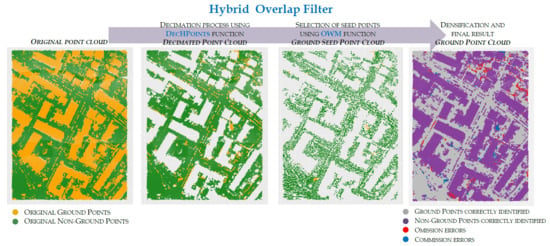
In order to test the efficacy of the decimation process using the DecHPoints function, a bar diagram (Figure 8) was constructed showing the original number of points (in green), the points remaining after the decimation process (in orange), and those selected as seed points (in pink), depending on whether they were ground points (P) or non-ground points (P). The values of Te and K were also included for each sample. The Figure 9 shows the qualitative results of our point decimation method using the ISPRS reference samples. In this figure, the spatial distribution of the original, decimated, and seed points is shown for Samples 11 (Figure 9a–c) and 41 (Figure 9d–f), which included buildings and/or vegetation. The results included in Figure 8 and Figure 9 were obtained from the optimal combination of parameters for each sample (Figure 6).
In general, the decimation process was more effective for urban samples than for rural samples (in 6 of the 9 urban samples, K was higher than 80%; this level of precision was only obtained for 15% of the rural samples). These results were expected as the aim of the decimation process was to eliminate non-ground points corresponding to buildings, which occurred in a higher proportion in urban samples than in rural samples (in urban zones, there were 1.1 ground points for each non-ground point, whereas in rural zones, the corresponding mean value was 7.8; Table 3).
In urban areas, the decimation process was most effective in areas of low relief, with the presence of large buildings (K = 89.53% and K = 95.11%), bridges (K = 91.32%), or discontinuities in the data (K = 96.29%; Figure 9e). However, our decimation method did not cope particularly well with areas of complex relief and including large buildings, terraces, and/or low vegetation (K = 51.54% (Figure 9b) and K = 66.31%). In the case of Sample 11, the low precision may be due to the presence of large buildings on different levels of terrain, so that the local maxima analyzed may correspond to ground and not to objects, thus simultaneously increasing both the omission and commission errors. However, this limitation did not apply to Sample 41, which included large buildings located in a flat area (K = 96.29%, Figure 9e). In the rural zones, the existence of a higher percentage of non-ground points in low vegetation led to the decimation process being less effective, giving rise to a low level of precision on hillside areas with vegetation (K = 60.49% and K = 49.58%). Furthermore, the lack of efficacy of the decimation process was also due to omission errors, mainly at the edges of gullies (K = 45.87% and K = 51.85%) or embankments beside roads (K = 71.45%).
3.4.3. Influence of the OWM Method on the Selection of Ground Seed Points
As already mentioned, the OWM function uses a moving window with longitudinal and transverse overlap to select local lowest points. Thus, for an overlap of 80%, each point was analyzed 25 times, but only those points selected as local lowest points more than once during the process were considered seed points (P). Thus, it was expected that without increasing the number of commission errors, the number of seed points would be greater than with the LMM method, and the first estimate would be a better representation of the actual terrain relief. In addition, the results of using the OWM function may benefit from prior decimation of the point cloud as reducing the window size to a similar size as in rural zones would enable selection of a greater number of local lowest points.
In order to explore the above ideas further, the OWM function was applied, by way of example, to Samples 12 and 52, with a longitudinal and transverse overlap between samples of 0% (LO = FO = 0), thus simulating the LMM function. In addition, the function was also executed with an overlap of 80% (LO = FO = 0.8). Both the original point cloud (P) and the decimated point cloud (P) were considered. The qualitative results of this experiment are included in Figure 10. In general, at road edges and inner courtyards of buildings (Figure 10b compared with Figure 10c) and at the edges of water bodies (Figure 10h compared with Figure 10i), the surface was better defined by OWM than by LMM. Irrespective of whether the input data were decimated or not, the OWM function selected almost four times more points than the LMM method. Although the number of erroneously selected non-ground points was also higher, most of these points corresponded to low vegetation, and none of them corresponded to buildings. In addition, the mean percentage error (mean proportion of non-ground points as a function of the total number of seed points) was very similar for both methods (LMM = 1.1% vs. OWM = 0.9% using original point clouds and LMM = 0.65% vs. OWM = 0.75% using decimated point clouds). In both cases, the results were better than those obtained with other seed point selection methods (e.g., [36] and [37] reported that ≈4% and ≈2% of the automatically selected seed points were non-ground points, respectively). The use of OWM may lead to the investment of fewer resources in the posterior densification of the model.
The decimation process also had a positive influence on the input data, increasing the seed points by a factor 15 in Sample 12 and by a factor 20 in sample 52 relative to the results obtained from original point clouds. These results were possible as the size of window for selecting seed-points could be reduced from 18 m to 3 m in Sample 12 and from 26 m to 5 m in Sample 52. Although in the first case, the size of the window (3 m) was almost half of that in the second case (5 m) and the number of ground points was greater in Sample 12 (P = 26,654 in the original point cloud and P = 26,269 in decimated point clouds) than in Sample 52 (P = 20,112 in the original point cloud and P = 19, 300 in decimated point clouds), paradoxically, the number of seed points selected was greater in the latter than in the former case (using original point clouds: Seed points = 761, OP (Overall Precision (OP) is the rate of correctly classified ground points in all extracted ground seed points [37].) = 98.7%, and Seed points = 746, OP = 99.6%; using decimated point clouds: Seed points = 10038, OP = 99.1%, and Seed points = 15320, OP = 99.4%). This may be due to the fact that Sample 12 was more complex than Sample 52. In addition, the presence in the latter of two relatively flat zones with few non-ground points (upper and lower parts of the scene) may have favored the selection of seed points.
3.4.4. Influence of the Variable Parameters on the Filtering Accuracy
The quantitative results of the parameter fitting described in Section 3.3 were used to study the influence of the variable parameters on the identification of ground points. Figure 11 includes representations of the variations in the values of the errors Te (Figure 11a), TIe (Figure 11b), and TIIe (Figure 11c) (vertical axis) with the values of the parameters C, C and (horizontal axis) for all samples (in grey), the urban samples (in purple), and the rural samples (in green). The value of the 68.3% percentile for each error is shown as a horizontal line. For simplified interpretation of the graphs, the influence of the variations on the value of each of the factors (variable parameters) would increase as the length of the vertical lines including the factor levels decrease.
Considering all samples (results shown in grey in Figure 11), fluctuations in parameter C had less effect than fluctuations in parameter C on TIIe and Te. As expected, the values of parameter C and TIe were directly related, i.e., the value of TIe decreased with the value of C, as the probability of selecting ground points increased as the value of C decreased. However, as a direct consequence of this relationship, the probability of erroneously selecting points that were not ground points also increased, thus increasing the TIIe, as reflected in Figure 11c, in which the values of parameters C decreased as those of TIIe increased. The inverse relationship between parameter C and TIIe also observed in this graph may be explained by the influence of the parameter during the decimation process, during which high values must be used in order to remove points corresponding to large buildings.
Analysis of the influence of parameter on the different types of error was carried out carefully, as 660 results were obtained by varying parameters C and C while = 0.5, compared with the 64 results obtained when the latter parameter was varied while maintaining each of the first two parameters constant. This may explain why the levels of parameter were not arranged in an orderly fashion along the vertical line on which they were represented. However, if we disregarded the 0.5 level, we see that as the value of increased, the values of TIe and Te decreased and that of TIIe increased. The explanation for this is the same as for the influence of parameter C on the different types of error.
Finally, the same analysis was carried out by considering the urban samples (Sample 11 to Sample 42 shown in purple) and the rural samples (Sample 51 to Sample 71 shown in green) to evaluate whether the type of environment generates different relationships between the variable parameters and the three types of error. The same pattern was observed for the urban samples as for all of the samples, although the influence of the variations in parameter C on the size of Te was more evident in the urban samples (Figure 11a). However, the same pattern was not observed for the rural samples, as the influence of parameter C on the values of Te was not very different from that of parameter C. Although analysis of all samples did not reveal a clear relationship between C and Te, separate analysis of the urban and rural samples revealed an inverse relationship, where the value of Te decreased as the value of C increased (Figure 11a).
In urban zones, the variations in C had much greater effect on TIIe than caused by variations in C, whereas in rural zones, the opposite was true (Figure 11c). One possible explanation for this finding was that in urban zones, most of the non-ground points corresponded to large buildings, whereas in rural zones, the non-ground points generally represented vegetation or small buildings. Thus, in urban zones, if the value of C was less than the size of the largest building in the zone, this would have various effects: first, the decimation process would fail for points corresponding to the roofs of buildings larger than the C value; some of these non-decimated non-ground points would be selected as seed points, and finally, many points corresponding to the roofs would be classified as ground points. Thus, a greater volume of points would be classified as ground points than when the error was associated with a smaller building or a vegetated zone (characteristic of rural zones), and TIIe would reach very high values, irrespective of the value of C. This phenomenon ceased to occur when the value of C was greater than the size of the buildings present in the zone, thus considerably decreasing the influence on TIIe.
3.5. Assessment of Filtering Accuracy
3.5.1. Quantitative and Qualitative Results of HyOF
The quantitative results regarding the precision of the HyOF evaluated using the 15 ISPRS reference samples and the metrics proposed by [23] are shown in Table 4. The table includes the values of the errors TIe, TIIe, and Te and the Kappa coefficient, obtained using the optimal parameters for each sample, as well as a single combination of parameters. The final row includes the errors obtained taking into account the points in all samples together. In previous studies, calculation of the global filtering precision was obtained from the arithmetic mean value of the errors for the 15 samples [8,38]. Although this was the simplest method, it did not take into account the proportion of points of each type relative to the total number of points. To overcome this deficiency, we used the total number of points in all study areas classified correctly and incorrectly as ground points and non-ground points. In addition, the Figure 12 shows the spatial distribution of the errors for Samples 11, 12, 41, 52, and 53 represented by the True Positives (TP), False Positives (FP), False Negatives (FN), and True Negatives (TN).
Regarding the optimal results, in 80% of the cases, Te was less than 5%, whereas K was higher than 88%. For all of the samples, Te and K were respectively 3.34% and 92.62%. For a single combination of parameters, the values of the same statistics were slightly lower, respectively 4.52% and 90.04%. Depending on the type of sample, our hybrid filter produced better results in urban zones (K = 92.18%) than in rural zones (K = 88.73%) (Table 5). In the first, most of the results were very satisfactory, mainly in environments with large buildings and small objects (K = 95.02%, Figure 12b (3DGraph), and K = 97.54% (3DGraph)), discontinuous data (K = 96.65%, Figure 12c (3DGraph) and K = 98.05% (3DGraph)), or the presence of bridges (K = 97.06% (3DGraph)). These good results were due to the high efficacy of the decimation process (Figure 8) as the removal of non-ground points corresponding to buildings enabled reduction of the size of the window (C) used to select the ground seed points, which enabled precise estimation of the terrain surface. As discussed earlier, in rural zones without large buildings, the decimation process was not as important as in urban zones.
By contrast, the poorest results were obtained for Samples 11 and 53 (using the optimal parameters Te = 10.64% and K = 62.21%). The errors in Sample 11 (Figure 12a (3DGraph)) were mainly due to the high number of false positives caused by the shallow sloping surface (southern part of the sample) and the erroneous identification of points corresponding to small objects and/or low vegetation (northern part of the sample). The errors were due to the low efficacy of the decimation process in terms of removing non-ground points (Figure 8 and Figure 9b). Sample 53 (Figure 12e (3DGraph)) corresponded to a rural zone where 95% of the points were ground points distributed on steep terrain with no buildings. The high percentage of ground points (23.8 ground points for each non-ground point; Table 3) caused the omission error (TIe = 2.89%) to have a much greater influence on the magnitude of Te and K than the commission error, even when TIIe > 20%. The main omission errors occurred at the breaklines, probably due to the accumulation of errors during the filtering process. First, errors would occur during the selection of ground seed points, as in these zones, the points would be selected in the lower part of the gully and not at the upper edge. Errors would then also occur during the densification process, as the thin plate spline interpolation tended to smooth these transition zones, leading to underestimation of the model elevation. Thus, the points at the upper edge would have much larger residual values than permitted, and therefore, these points would not be selected. The errors would be reduced, thus increasing the value of parameter ; however, this led to an increase in commission errors due to the presence of low vegetation. Most of the filters did not deal well with the characteristics of these areas, where the vegetation and buildings occurred on steep slopes and in precipitous areas [9,37,39].
3.5.2. Comparison with Other Filtering Algorithms
For comparison of the results obtained in the present study and those obtained with other filters, we considered 33 studies carried out between 1998 and 2019. The errors TIe and TIIe were represented in the scatter plots in Figure 13. In each case, the errors were obtained for each reference sample (in the studies of [8,12,24], as in the present study, the results were obtained using the optimal combination of parameters), whereas Table 5 includes the Kappa coefficient for each case; the last three columns include the results for all samples and for the urban and rural samples in each study. For the 33 studies, the K values were recalculated using the TIe, TIIe, and Te errors included in the different studies and the number of original ground points and non-ground points in each sample (Table 3).
Our hybrid filter was one of the four most precise filters (Table 5). The results produced were only surpassed by those obtained with the adaptive surface algorithm of [8] (Te = 2.87% and K = 93.63%), those of the morphological algorithm of [38] (Te = 3.01% and K = 93.33%), and those of the interpolation filter of [39] (Te = 3.15% and K = 93.00%). The precision of the algorithms increased greatly since the study carried out by [23] more than a decade ago. This was demonstrated by the fact that in the last few years, the results have improved for 75% of the samples (purple cells in Table 5). Our hybrid filter produced better results for three of the 15 samples than in the 33 previous studies. All algorithms produced better results in urban than in rural areas, with the exception of the filter implemented in TerraScan (K = 79.8% and K = 85.7%) and the hybrid filter of [37] (K = 81.7% and K = 85.2%). Although [4] attributed the better functioning of the TerraScan algorithm in these zones to the good quality of the input data, specifically the point density, it was possible that the selection of the filtering parameters was more important than the density of points. The algorithm implemented in TerraScan was an adapted version of the algorithm proposed by [41], who obtained a much higher K value in urban zones than that obtained by TerraScan (K = 90.1% and K = 79.8%).
The work in [23] reflected on which error should be reduced in order to improve the quality of the filter and increase the efficacy of the posterior correction tasks. They concluded that they should minimize the TIe based on the cost of committing this error in relation to the application of the final model and of the model manually decimated of these errors. This condition was fundamentally met in areas where the number of ground points was significantly higher than the number of non-ground points (P/P»>1). In these cases, TIe had a much greater influence than TIIe on the overall precision of the filtering process than if the number of ground points and non-ground points were more balanced (P/P≈1). In the first case, in Samples 53 and 61 (23.8 and 28.1 ground points for each non-ground points, respectively; Table 3), more than 95% of the points corresponded to ground points. Regarding Sample 53, the algorithms developed up to 2004 yielded a much higher TIe and a lower TIIe than in the other cases, whereas the latter was much higher in the algorithms developed in the last decade. As a result, for this sample and others with similar characteristics, the value of Te increased with that of TIe.
The aforementioned reflection may be due to the fact that the algorithms included in the study of [23] aimed to minimize TIIe rather than TIe (Figure 13a). However, the filters developed in the last decade minimized TIe at the cost of increasing the commission errors (Figure 13b–d). Considering the results of the first eight algorithms together produced mean values of the omission and commission errors of respectively 17.5% and 2.4%, compared with values of 5.0% and 5.6% produced by the filters developed since 2004. This could be observed in Figure 13a–d. There were some exceptions within the latter group of algorithms, such as that used by [25], in which many of the values of TIIe were lower than those of TIe (considering all samples: TIe = 15.34% and TIIe = 4.86%). These authors minimized the commission errors as they considered that they produced more negative effects in the final model than the omission errors, which simply reduced the level of detail with which the terrain was represented [38].
Although these findings contrasted with the trends observed in recent years, these authors made a very interesting observation that reinforced their position. They considered that a point that was wrongly classified as ground would have a greater impact on the final model if it corresponded to a roof than if it corresponded to low vegetation. This impact would be much greater if the point were added at the seed selection stage than during the densification process. Therefore, the reflection of [23] could be qualified by considering that TIe should be minimized in order to increase the general precision of the filtering process, although at the risk of increasing TIIe, as long as the commission errors were not due to the incorrect selection of points corresponding to the roofs of buildings. Our hybrid filter complied with this requisite thanks to the efficacy of the decimation process in built-up areas (magenta squares in Figure 13d). Finally, the considerations of [23] were aimed at improving the filtering precision, whereas those of [25] were focused on improving the model precision. In most cases, an increase in the filtering precision was generally accompanied by an increase in the precision of the final model; however, although apparently contradictory, this was not always the case.
Other authors also mentioned that the aforementioned tendency was fundamentally due to the process of densification included in some filters [8]. On the one hand, they attributed the increase in TIIe to the fact that the number of non-ground points was much lower than the number of ground points in some samples (e.g., Samples 53 and 61) and that the erroneous classification of few non-ground points as ground points led to a high TIIe. However, it was possible that the main reason was not the number of points, but the type of surface they represented (in most cases, low vegetation), along with the location on rough terrain. These authors also associated the errors with the densification strategy used in the filters, which was closely related to the previously mentioned point. For steep terrain, these filters tended to assign high values to the parameter controlling the densification process, with the aim of decreasing the number of omission errors. For example, in the present study, for Sample 53, parameter reached its maximum value (0.8 m) as did TIIe (20.59%). For the same sample, in the study of [24], the parameter TH (height threshold) also reached its maximum value (2.6 m), and TIIe reached the maximum value of 33.5%; in a similar way, the adaptive surface filter of [8] produced a commission error of 38.75% when the max-bend-gain parameter took a maximum value of 1 m.
Finally, as reported by [8,12,24], the precision of our hybrid filter was calculated using a single combination of parameters (C = 4, = 0.5 and C = 30 for urban samples and C = 20 for rural samples). The use of this combination of parameters confirmed the robustness of our hybrid filter regarding different terrain characteristics (K = 90.04%). However, some differences were observed in relation to the type of sample, with the urban samples producing fewer fluctuations than in the optimal results obtained for the rural samples (mean difference of K = 2.2% and mean difference of K = 6.7%: data obtained from the results in Table 5). This trend was evident in the studies of [24] and [8], but not in that of [12], in which the minimal differences indicated the robustness in response to variations in the parameters.
4. Conclusions
The identification of ground points in LiDAR point clouds is an extremely complex process. Despite the great effort that has been made to solve this problem, simplifying the process remains a challenge, in terms of both effectivity and usability/accessibility. This article presented a new filtering algorithm, HyOF, which was comprised of various functions implemented in the free R software environment. The algorithm was a hybrid filter that combined a decimation process (DecHPoints function), which aimed to remove points corresponding to buildings, along with a new method for selecting seed points (OWM) and an iterative densification process. The main conclusions of the study were grouped into six blocks coinciding with the different points analyzed in the Results and Discussion Section.
Parameter tuning: Although the identification of optimal parameters was a tedious and time-consuming task, the input of effort was compensated by an increase in the filtering effectivity. In this study, the use of the optimal combination of parameters for each sample increased the overall filtering precision by more than 2.5 percentage points (considering all samples: K = 92.62% and K = 90.04%). The analysis conducted may serve as a reference point and simplifying parameter optimization in other regions.
Effectiveness of the decimation process: Due to its characteristics, our point decimation method was more effective in urban zones (in 70% of cases, the value of K was greater than 80%) than in rural zones, where the same level of precision was only obtained in 15% of the instances. Although the function had some limitations regarding the presence of small objects or buildings on the hillside, the decimation process was generally effective, and its use in combination with other filters may improve the results of these.
Influence of the OWM function on the selection of seed points: Our method for selecting ground seed points proved versatile in relation to its ability to be executed like the Local Minimum Method (LMM) and also its effectivity in identifying seed points, selecting up to four times more points than the LMM. In addition, use of the OWM together with our point decimation method enabled selection of up to 20 times more seed points than when the original point cloud was used. Use of this method contributed to overcoming some of the structures with which the filters did not perform well, such as inner courtyards or zones close to fault lines or gullies. As in the previous case, we believe that the result of many filters could be improved by using the OWM method to select the seed points. Filters that could be improved include those that require the seed points to generate the original reference surface and also those that use the seed points as a basis for classifying new ground points from differences in elevation.
Influence of the variable parameters on the filtering precision: In all cases, C was directly related to TIe and inversely related to TIIe. Finding a value of parameter C that yielded an equilibrium between TIe and TIIe was therefore challenging. Potential users should note that the main conclusion of the analysis carried out to determine the influence of the type of environment on the variable parameters and the errors was that for urban zones, particular attention should be given to the value of parameter C, which significantly affected Te, whereas parameter C was more important in rural zones.
Filtering results: Taking into account the 15 reference samples provided by the ISPRS and the optimal combinations of parameters, our hybrid filtering method, HyOF, yielded Te = 3.34% and K = 92.62%, whereas use of a single combination yielded Te = 4.52% and K = 90.04%. Regarding the different types of environments, better results were obtained in urban zones (K = 92.18%) than in rural zones (K = 88.73%), and the performance of the algorithm was more robust in response to fluctuations in the variable parameters in the former (K = 90.02%) than in the latter (K = 82.39%). Regarding the origin and spatial location of the errors, irrespective of the environment, most filtering errors were produced in fault lines in areas such as gullies, ditches, and/or embankments. Some of the omission errors may have originated from the definition of the ground and from the study objectives. Previous studies showed that the definition may not be entirely adequate as, e.g., some applications may wish to consider ramps as objects or bridges as ground or vice versa. These elements would therefore have to be specifically detected and the user allowed to establish whether they should be considered ground.
Comparison with other filtering algorithms: In the last few years, the results have been improved for almost 75% of the reference samples, and 30% of the improved results were obtained using our hybrid filtering method and the optimal combination of parameters. The algorithm generally proved very effective as it was among the four most precise in a total of 33 studies. The current trend in developing filtering algorithm is to minimize the TIe. This was clearly demonstrated by the results produced by the algorithms developed in the last decade, where TIe = 5.0% and TIIe = 5.6%, compared with TIe = 17.5% and TIIe = 2.4% for the results produced by the algorithms used up to 2004. Considering the results for all samples and using the optimal combinations of parameters, our hybrid filtering method continued this trend, yielding TIe = 2.62% and TIIe = 4.70%.
As a final reflection, we believe that in a society advancing towards the democratization of information and collaborative processes, researchers should not only focus on improving the efficacy of the processing tools, but should also consider the users’ needs with a view toward improving the usability and accessibility of these tools in order to develop a process that will provide solutions to the actual challenges.
Author Contributions
Conceptualization, S.B., M.C., and D.M.; methodology, S.B., M.C., and D.M.; software, S.B.; validation, S.B.; formal analysis, S.B.; investigation, S.B.; resources, S.B. and M.C.; data curation, M.C.; writing, original draft preparation, S.B., M.C., and D.M.; writing, review and editing, S.B., M.C., and D.M.; visualization, S.B.; supervision, D.M.; project administration, D.M.; funding acquisition, M.C. and D.M. All authors read and agreed to the published version of the manuscript.
Funding
This research was funded by the Project Red de Tecnoloxías LiDAR e de Información Xeoespacial (Plan Galego 2011–2015 (Plan I2C): Programa Consolidación e Estructuración (Redes)-CN 2012/323).
Acknowledgments
We are grateful to our colleagues at LaboraTe for their help and input, without which this study would not have been possible.
Conflicts of Interest
The authors declare no conflict of interest. The funders had no role in the design of the study; in the collection, analyses, or interpretation of data; in the writing of the manuscript; nor in the decision to publish the results.
Abbreviations
The following abbreviations are used in this manuscript:
| DecHPoints | Decimation of Highest Points |
| FO | Forward Overlap |
| HyOF | Hybrid Overlap Filter |
| LLP | Local Lowest Point |
| LMM | Local Minimum Method |
| LO | Lateral Overlap |
| OWM | Overlap Window Method |
References
- Moreira, J. La cartografía hoy: Evolución o revolución?. Las nuevas tecnologías y los cambios en la representación del territorio. In Actas del Congreso Año mil, año dos mil. Dos milenios en la Historia de España; Sociedad Estatal España Nuevo Milenio: Madrid, Spain, 2001; Volume 2, pp. 433–451. [Google Scholar]
- Li, Z.; Zhu, C.; Gold, C. Digital Terrain Modeling: Principles and Methodology; CRC Press: Boca Raton, FL, USA, 2005. [Google Scholar]
- Ullrich, A.; Hollaus, M.; Briese, C.; Doneus, W.W.; Mücke, W. Improvements in DTM generation by using full-waveform Airborne Laser Scanning data. In Proceedings of the 7th International Conference on “Laser Scanning and Digital Aerial Photography. Today and Tomorrow”, Moscow, Russia, 6–7 December 2007; Volume 6, pp. 1–9. [Google Scholar]
- Mongus, D.; Žalik, B. Parameter-free ground filtering of LiDAR data for automatic DTM generation. ISPRS J. Photogramm. Remote Sens. 2012, 67, 1–12. [Google Scholar] [CrossRef]
- Flood, M. LiDAR activities and research priorities in the commercial sector. Int. Arch. Photogramm. Remote Sens. 2001, 34, 3–8. [Google Scholar]
- Renslow, M. Manual of Airborne Topographic Lidar; American Society for Photogrammetry and Remote Sensing: Bethesda, MD, USA, 2012; p. 884. [Google Scholar]
- Chen, H.; Cheng, M.; Li, J.; Liu, Y. An iterative terrain recovery approach to automated DTM generation from airborne LIDAR point clouds. Int. Arch. Photogramm. Remote Sens. Spat. Inf. Sci. 2012, 39, 363–368. [Google Scholar] [CrossRef] [Green Version]
- Hu, H.; Ding, Y.; Zhu, Q.; Wu, B.; Lin, H.; Du, Z.; Zhang, Y.; Zhang, Y. An adaptative surface filter for airborne laser scanning point clouds by means of regularization and bending energy. ISPRS J. Photogramm. Remote Sens. 2014, 92, 98–111. [Google Scholar] [CrossRef]
- Yang, B.; Huang, R.; Dong, Z.; Zang, Y.; Li, J. Two-step adaptive extraction method for ground points and breaklines from lidar point clouds. ISPRS J. Photogramm. Remote Sens. 2016, 119, 373–389. [Google Scholar] [CrossRef]
- Maguya, A.S.; Junttila, V.; Kauranne, T. Adaptive algorithm for large scale dtm interpolation from lidar data for forestry applications in steep forested terrain. ISPRS J. Photogramm. Remote Sens. 2013, 85, 74–83. [Google Scholar] [CrossRef]
- Silván-Cárdenas, J.; Wang, L. A multi-resolution approach for filtering LiDAR altimetry data. ISPRS J. Photogramm. Remote Sens. 2006, 61, 11–22. [Google Scholar] [CrossRef]
- Shao, Y.C.; Chen, L.C. Automated Searching of Ground Points from Airborne Lidar Data Using a Climbing and Sliding Method. Photogramm. Eng. Remote Sens. 2008, 74, 625–635. [Google Scholar] [CrossRef] [Green Version]
- Hui, Z.; Hu, Y.; Yevenyo, Y.Z.; Yu, X. An Improved Morphological Algorithm for Filtering Airborne LiDAR Point Cloud Based on Multi-Level Kriging Interpolation. Remote Sens. 2016, 8, 35. [Google Scholar] [CrossRef] [Green Version]
- Yuan, F.; Zhang, J.-X.; Zhang, L.; Gao, J.-X. Urban DEM generation from airborne Lidar data. In 2009 Urban Remote Sensing Joint Event; IEEE: Shanghai, China, 2009; pp. 1–5. [Google Scholar]
- Yuan, F.; Zhang, J.; Zhang, L.; Gao, J. DEM generation from airborne LIDAR data. Int. Arch. Photogramm. Remote Sens. Spat. Inf. Sci. 2009, 38, 308–312. [Google Scholar]
- Lin, X.; Zhang, J. Segmentation-Based Filtering of Airborne LiDAR Point Clouds by Progressive Densification of Terrain Segments. Remote Sens. 2014, 6, 1294–1326. [Google Scholar] [CrossRef] [Green Version]
- Zhang, J.; Lin, X. Filtering airborne LiDAR data by embedding smoothness-constrained segmentation in progressive TIN densification. ISPRS J. Photogramm. Remote Sens. 2013, 81, 44–59. [Google Scholar] [CrossRef]
- Axelsson, P. DEM generation from laser scanner data using adaptive TIN models. Int. Arch. Photogramm. Remote Sens. 2000, 33, 111–118. [Google Scholar]
- Tóvári, D.; Pfeifer, N. Segmentation based robust interpoation—A new approach to laser data filtering. In Proceedings of the ISPRS WG III/3, III/4, V/3 Workshop “Laser scanning 2005”, Enschede, The Netherlands, 12–14 September 2005; pp. 79–84. [Google Scholar]
- Buján, S.; Sellers, C.A.; Cordero, M.; Miranda, D. DecHPoints: A new tool for improving LiDAR data filtering in urban areas. J. Photogramm. Remote Sens. Geoinf. Sci. 2020. [Google Scholar] [CrossRef]
- Chen, Z.; Gao, B.; Devereux, B. State-of-the-art: DTM generation using airborne LIDAR data. Sensors 2017, 17, 150. [Google Scholar] [CrossRef] [PubMed] [Green Version]
- Véga, C.; Durrieu, S.; Morel, J.; Allouis, T. A sequential iterative dual-filter for Lidar terrain modeling optimized for complex forested environments. Comput. Geosci. 2012, 44, 31–41. [Google Scholar] [CrossRef]
- Sithole, G.; Vosselman, G. Experimental comparison of filter algorithms for bare-Earth extraction from airborne laser scanning point clouds. ISPRS J. Photogramm. Remote Sens. 2004, 59, 85–101. [Google Scholar] [CrossRef]
- Chang, L.D. Bare-Earth Extraction and Vehicle Detection in Forested Terrain from Airborne Lidar Point Clouds. Ph.D. Thesis, University of Florida, Gainesville, FL, USA, 2010. [Google Scholar]
- Lu, W.L.; Little, J.J.; Sheffer, A.; Fu, H. Deforestation: Extracting 3D Bare-Earth Surface from Airborne LiDAR Data. In Proceedings of the Canadian Conference on Computer and Robot Vision, 2008. CRV ’08, Windsor, ON, Canada, 28–30 May 2008; pp. 203–210. [Google Scholar]
- ISO 9241-11. Ergonomic Requirements for Office Work with Visual Display Terminals (VDT)s—Part 11 Guidance on Usability; ISO: Geneva, Switzerland, 1998. [Google Scholar]
- Hassan, Y.; Fernández, F.J.M.; Iazza, G. Diseño Web Centrado en el Usuario: Usabilidad y Arquitectura de la Información. Hipertext.net 2004. No 2. Available online: http://hdl.handle.net/10760/8998 (accessed on 10 April 2019).
- R Development Core Team. R: A Language and Environment for Statistical Computing; R Development Core Team: Vienna, Austria, 2010. [Google Scholar]
- Chen, C.; Li, Y.; Li, W.; Dai, H. A multiresolution hierarchical classification algorithm for filtering airborne LiDAR data. ISPRS J. Photogramm. Remote Sens. 2013, 82, 1–9. [Google Scholar] [CrossRef]
- Chen, C.; Li, Y. A robust method of thin plate spline and its application to DEM construction. Comput. Geosci. 2012, 48, 9–16. [Google Scholar] [CrossRef]
- Evans, J.S.; Hudak, A.T. A multiscale curvature algorithm for classifying discrete return LiDAR in forested environments. IEEE Trans. Geosci. Remote Sens. 2007, 45, 1029–1038. [Google Scholar] [CrossRef]
- Sithole, G.; Vosselman, G. Report: ISPRS Comparison of Filters; Technical Report, ISPRS, Commission III, Working Group 3; Delft University of Technology: Delft, The Netherlands, 2003. [Google Scholar]
- Meng, X.; Currit, N.; Zhao, K. Ground filtering algorithms for airborne LiDAR data: A review of critical issues. Remote Sens. 2010, 2, 833–860. [Google Scholar] [CrossRef] [Green Version]
- Cohen, J. A coefficient of agreement for nominal scales. Educ. Psychol. Meas. 1960, 20, 37–46. [Google Scholar] [CrossRef]
- Susaki, J. Adaptive slope filtering of airborne LiDAR data in urban areas for Digital Terrain Model (DTM) generation. Remote Sens. 2012, 4, 1804–1819. [Google Scholar] [CrossRef] [Green Version]
- Jahromi, A.B.; Zoej, M.J.V.; Mohammadzadeh, A.; Sadeghian, S. A novel filtering algorithm for bare-earth extraction from airborne laser scanning data using an artificial neural network. IEEE J. Sel. Top. Appl. Earth Obs. Remote Sens. 2011, 4, 836–843. [Google Scholar] [CrossRef]
- Cai, S.; Zhang, W.; Liang, X.; Wan, P.; Qi, J.; Yu, S.; Yan, G.; Shao, J. Filtering Airborne LiDAR Data Through Complementary Cloth Simulation and Progressive TIN Densification Filters. Remote Sens. 2019, 11, 1037. [Google Scholar] [CrossRef] [Green Version]
- Pingel, T.J.; Clarke, K.C.; McBride, W.A. An improved simple morphological filter for the terrain classification of airborne LIDAR data. ISPRS J. Photogramm. Remote Sens. 2013, 77, 21–30. [Google Scholar] [CrossRef]
- Chen, C.; Li, Y.; Zhao, N.; Guo, J.; Liu, G. A fast and robust interpolation filter for airborne lidar point clouds. PLoS ONE 2017, 12, e0176954. [Google Scholar] [CrossRef] [Green Version]
- Pfeifer, N.; Kostli, A.; Kraus, K. Interpolation and filtering of laser scanner data—Implementation and first results. Int. Arch. Photogramm. Remote Sens. 1998, 32 Pt 3/1, 31–36. [Google Scholar]
- Axelsson, P. Processing of laser scanner data—Algorithms and applications. ISPRS J. Photogramm. Remote Sens. 1999, 54, 138–147. [Google Scholar] [CrossRef]
- Elmqvist, M.; Jungert, E.; Lantz, F.; Persson, A.; Soderman, U. Terrain modelling and analysis using laser scanner data. Int. Arch. Photogramm. Remote Sens. 2001, 34, 219–226. [Google Scholar]
- Roggero, M. Airborne laser scanning: Clustering in raw data. Int. Arch. Photogramm. Remote Sens. 2001, 34, 227–232. [Google Scholar]
- Sithole, G. Filtering of laser altimetry data using a slope adaptive filter. Int. Arch. Photogramm. Remote Sens. Spat. Inf. Sci. 2001, 34, 203–210. [Google Scholar]
- Brovelli, M.A.; Cannata, M.; Longoni, U.M. Managing and processing LIDAR data within GRASS. In Proceedings of the GRASS Users Conference, Trento, Italy, 11–13 September 2002; Volume 29, pp. 1–29. [Google Scholar]
- Sohn, G.; Dowman, I. Terrain surface reconstruction by the use of tetrahedron model with the MDL criterion. Int. Arch. Photogramm. Remote Sens. Spat. Inf. Sci. 2002, 34 Pt 3/A, 336–344. [Google Scholar]
- Wack, R.; Wimmer, A. Digital terrain models from airborne laserscanner data-a grid based approach. Int. Arch. Photogramm. Remote Sens. Spat. Inf. Sci. 2002, 34 Pt 3/B, 293–296. [Google Scholar]
- Yan, M.; Blaschke, T.; Liu, Y.; Wu, L. An object-based analysis filtering algorithm for airborne laser scanning. Int. J. Remote Sens. 2012, 33, 7099–7116. [Google Scholar] [CrossRef]
- Li, Y. Filtering Airborne LiDAR Data by an Improved Morphological Method Based on Multi-Gradient Analysis. Int. Arch. Photogramm. Remote Sens. Spat. Inf. Sci. 2013, 40 Pt 1/W1, 191–194. [Google Scholar] [CrossRef] [Green Version]
- Li, Y.; Yong, B.; Wu, H.; An, R.; Xu, H. An Improved Top-Hat Filter with Sloped Brim for Extracting Ground Points from Airborne Lidar Point Clouds. Remote Sens. 2014, 6, 12885–12908. [Google Scholar] [CrossRef] [Green Version]
- Mongus, D.; Žalik, B. Computationally Efficient Method for the Generation of a Digital Terrain Model From Airborne LiDAR Data Using Connected Operators. IEEE J. Sel. Top. Appl. Earth Obs. Remote Sens. 2014, 7, 340–351. [Google Scholar] [CrossRef]
- Zhang, W.; Qi, J.; Wan, P.; Wang, H.; Xie, D.; Wang, X.; Yan, G. An easy-to-use airborne LiDAR data filtering method based on cloth simulation. Remote Sens. 2016, 8, 501. [Google Scholar] [CrossRef]
- Li, Y.; Yong, B.; Van Oosterom, P.; Lemmens, M.; Wu, H.; Ren, L.; Zheng, M.; Zhou, J. Airborne LiDAR Data Filtering Based on Geodesic Transformations of Mathematical Morphology. Remote Sens. 2017, 9, 1104. [Google Scholar] [CrossRef] [Green Version]
- Nie, S.; Wang, C.; Dong, P.; Xi, X.; Luo, S.; Qin, H. A revised progressive TIN densification for filtering airborne LiDAR data. Measurement 2017, 104, 70–77. [Google Scholar] [CrossRef]
- Wang, L.; Xu, Y.; Li, Y. Aerial Lidar Point Cloud Voxelization with its 3D Ground Filtering Application. Photogramm. Eng. Remote Sens. 2017, 83, 95–107. [Google Scholar] [CrossRef]
- Ni, H.; Lin, X.; Zhang, J.; Chen, D.; Peethambaran, J. Joint Clusters and Iterative Graph Cuts for ALS Point Cloud Filtering. IEEE J. Sel. Top. Appl. Earth Obs. Remote Sens. 2018, 11, 990–1004. [Google Scholar] [CrossRef]
- Hui, Z.; Li, D.; Jin, S.; Ziggah, Y.Y.; Wang, L.; Hu, Y. Automatic DTM extraction from airborne LiDAR based on expectation-maximization. Opt. Laser Technol. 2019, 112, 43–55. [Google Scholar] [CrossRef]
Figure 1.
The type of filtering methods developed between 1996 and 2016.

Figure 2.
Selection of the local lowest points using the OWM function. LLP, Local Lowest Point.

Figure 3.
PNTpseudo-code.

Figure 4.
Decimation of Highest Points function (DecHPoints) pseudo-code.

Figure 5.
HyOF pseudo-code.

Figure 6.
Values of the automatic and variable HyOF parameters.

Figure 7.
Efficacy of the penetrability during the decimation process (urban samples: magenta-purple boxes; rural samples: orange boxes; all samples: blue box).
Figure 7.
Efficacy of the penetrability during the decimation process (urban samples: magenta-purple boxes; rural samples: orange boxes; all samples: blue box).

Figure 8.
Effectiveness of DecHPoints function (original points are represented in green, decimated-point cloud in orange, and seed points in pink).
Figure 8.
Effectiveness of DecHPoints function (original points are represented in green, decimated-point cloud in orange, and seed points in pink).

Figure 9.
Qualitative results of the DecHPoints function (ground points in green and non-ground points in yellow). Examples: (a–c) are the results of Sample 11 and (d–f) the results of Sample 41.
Figure 9.
Qualitative results of the DecHPoints function (ground points in green and non-ground points in yellow). Examples: (a–c) are the results of Sample 11 and (d–f) the results of Sample 41.

Figure 10.
Comparison of the results of the Local Minimum Method (LMM) and OWM of selecting seed points from original point clouds and decimated point clouds for Samples 12 (a–f)) and 52 (g–l)).
Figure 10.
Comparison of the results of the Local Minimum Method (LMM) and OWM of selecting seed points from original point clouds and decimated point clouds for Samples 12 (a–f)) and 52 (g–l)).

Figure 11.
Influence of the variable parameters on the quality of the filtering process, considering all samples (in grey), the urban samples (Sample 11 to sample 42, in purple), and the rural samples (Sample 51 to sample 71, in green) using (a) total error; (b) Type I error, and (c) Type II error.
Figure 11.
Influence of the variable parameters on the quality of the filtering process, considering all samples (in grey), the urban samples (Sample 11 to sample 42, in purple), and the rural samples (Sample 51 to sample 71, in green) using (a) total error; (b) Type I error, and (c) Type II error.

Figure 12.
Qualitative results of the proposed hybrid method.

Figure 13.
Comparison of the TIe and TIIe obtained in the present study (magenta squares in (d)) and those obtained with other filters from all samples.
Figure 13.
Comparison of the TIe and TIIe obtained in the present study (magenta squares in (d)) and those obtained with other filters from all samples.


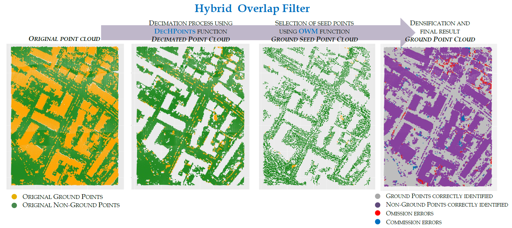
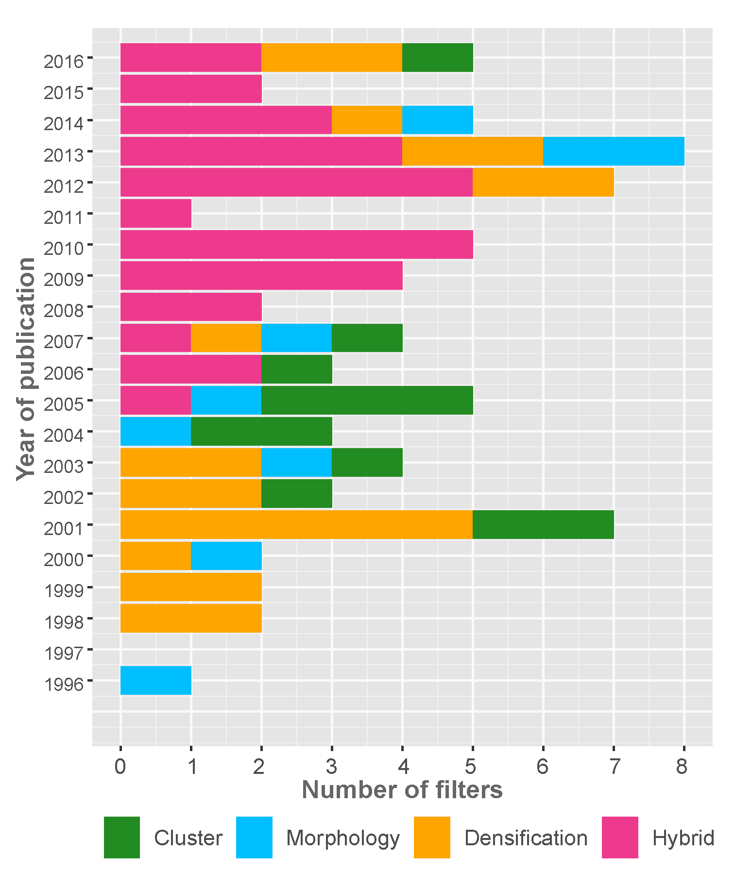
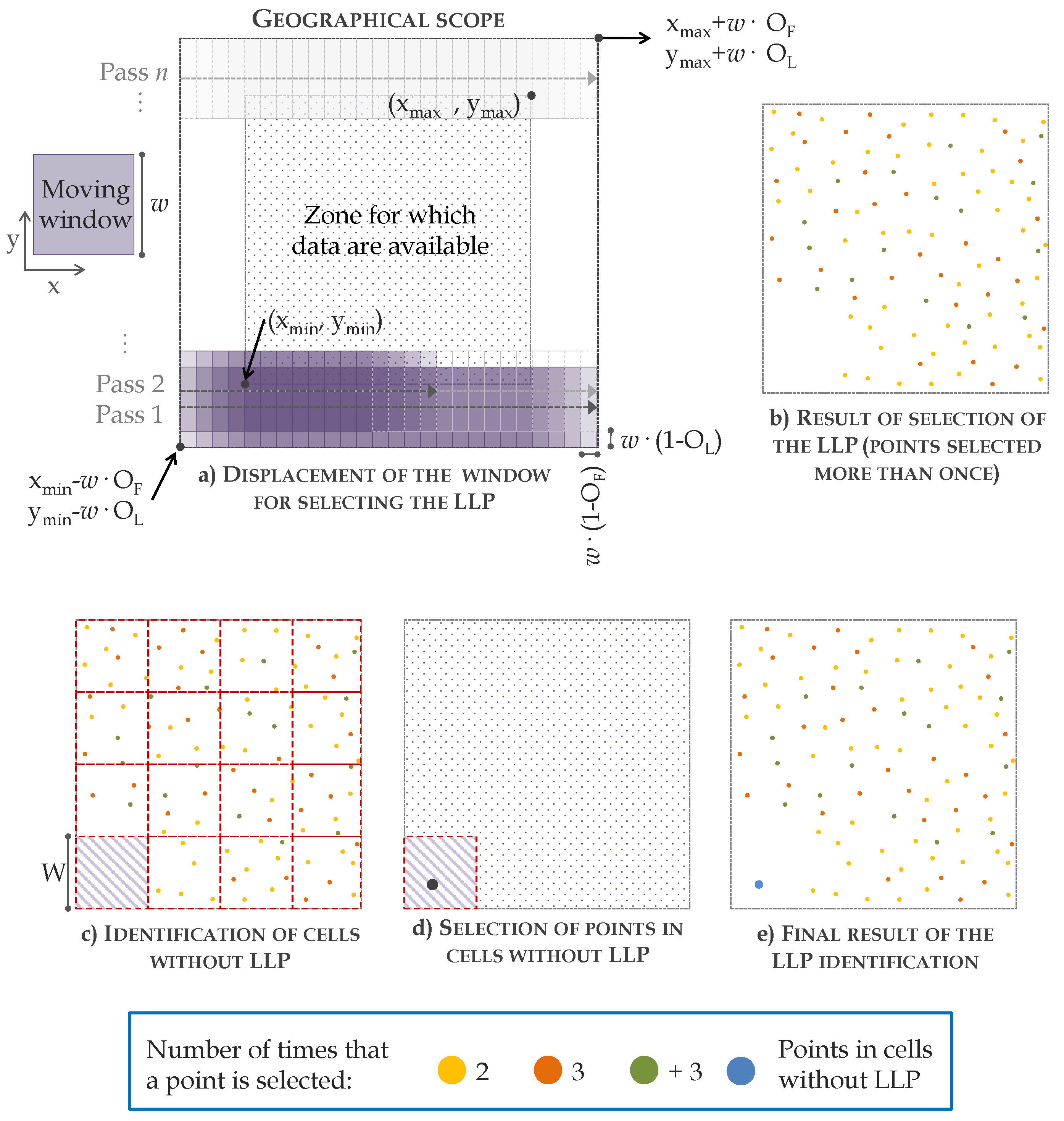
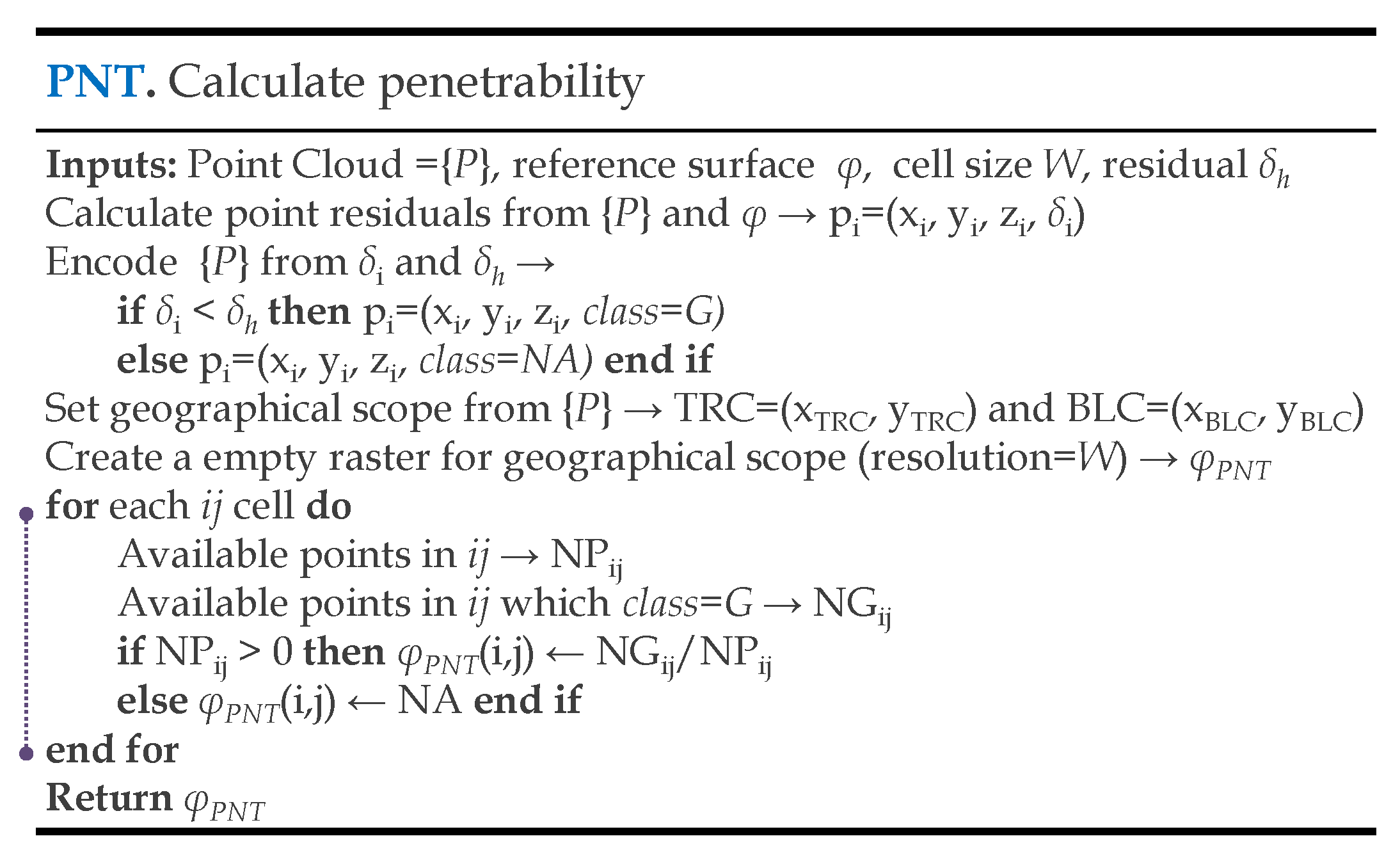
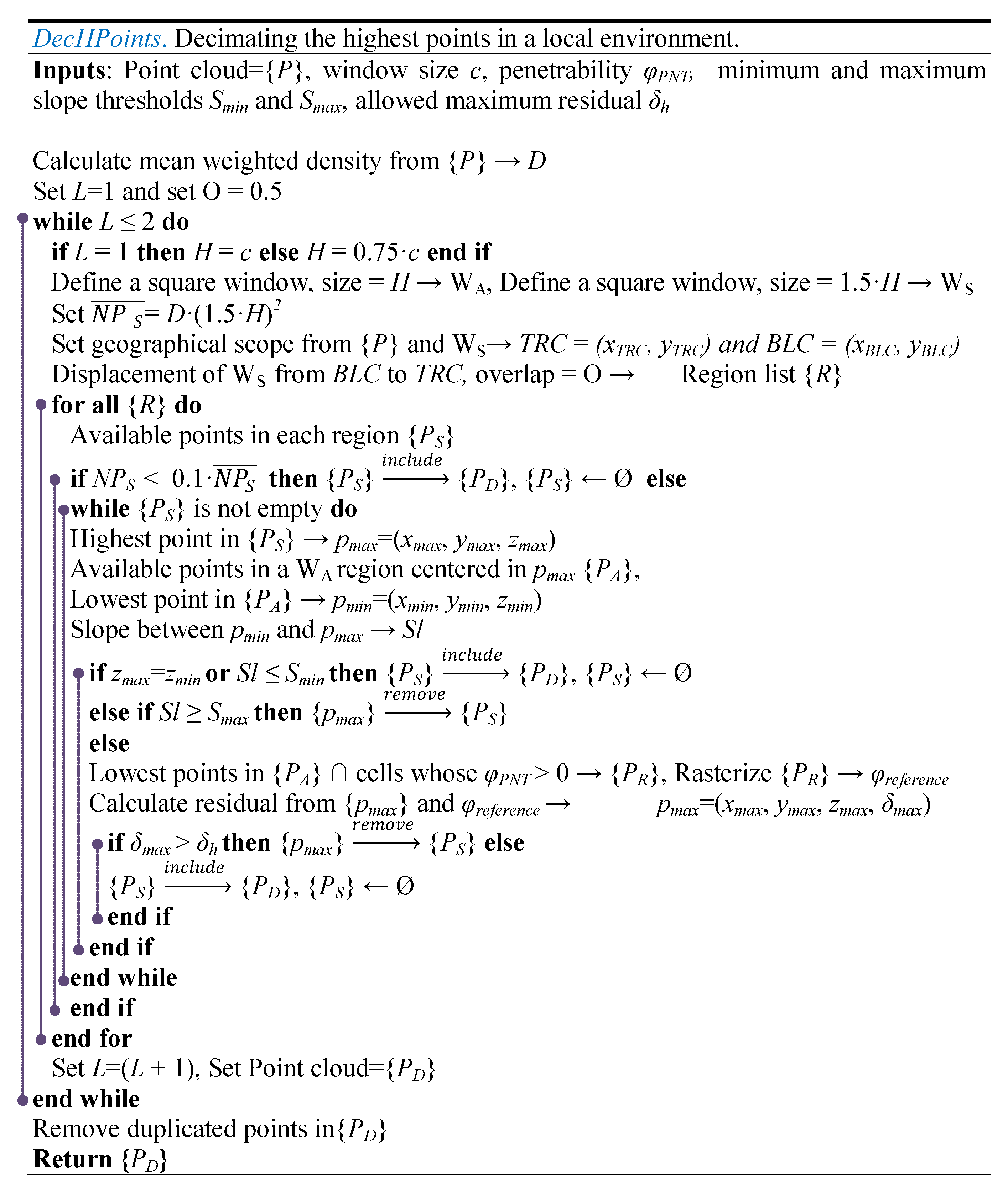
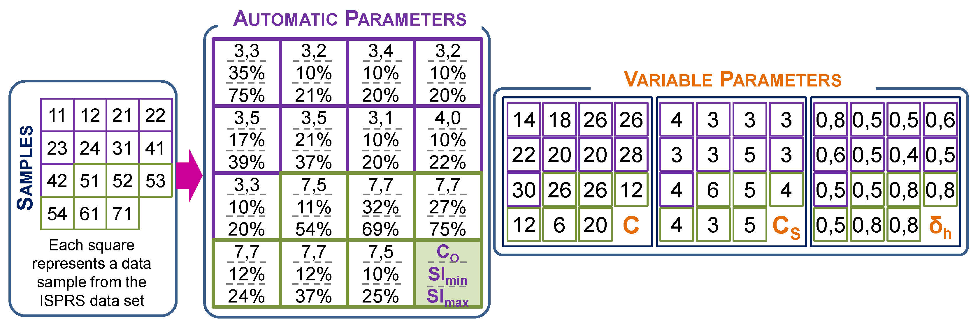
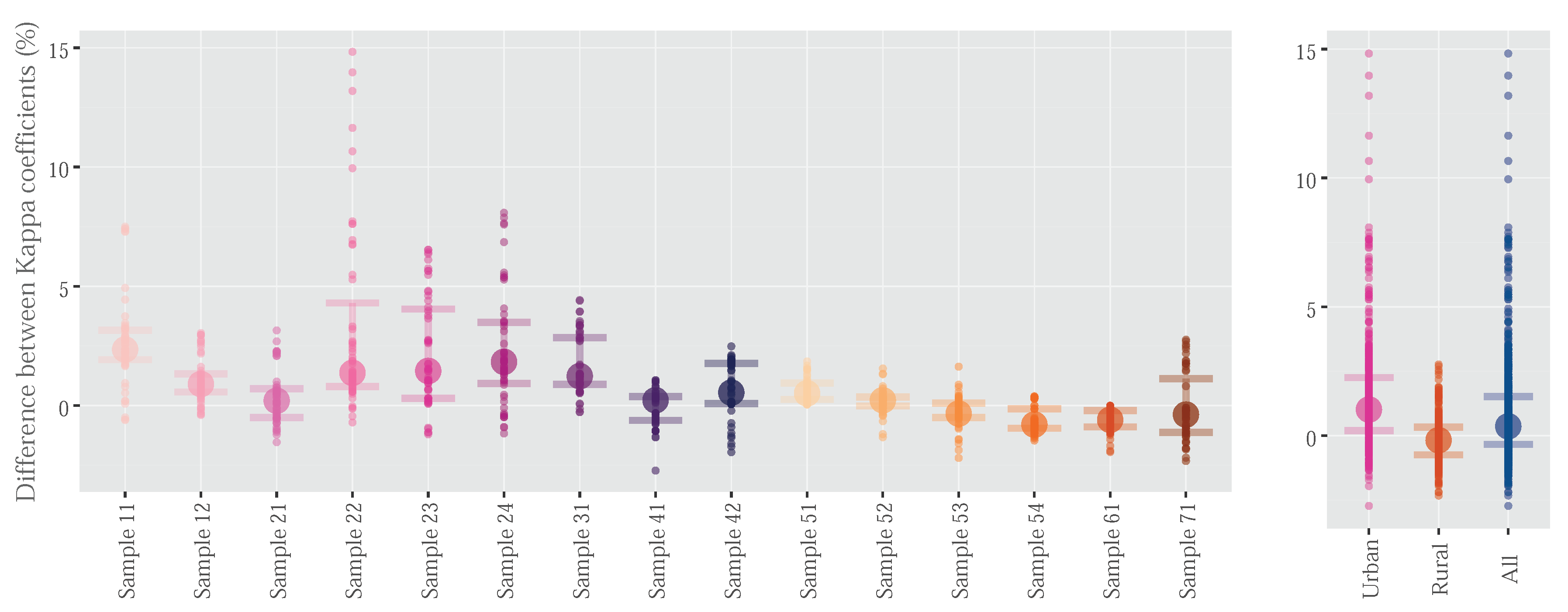
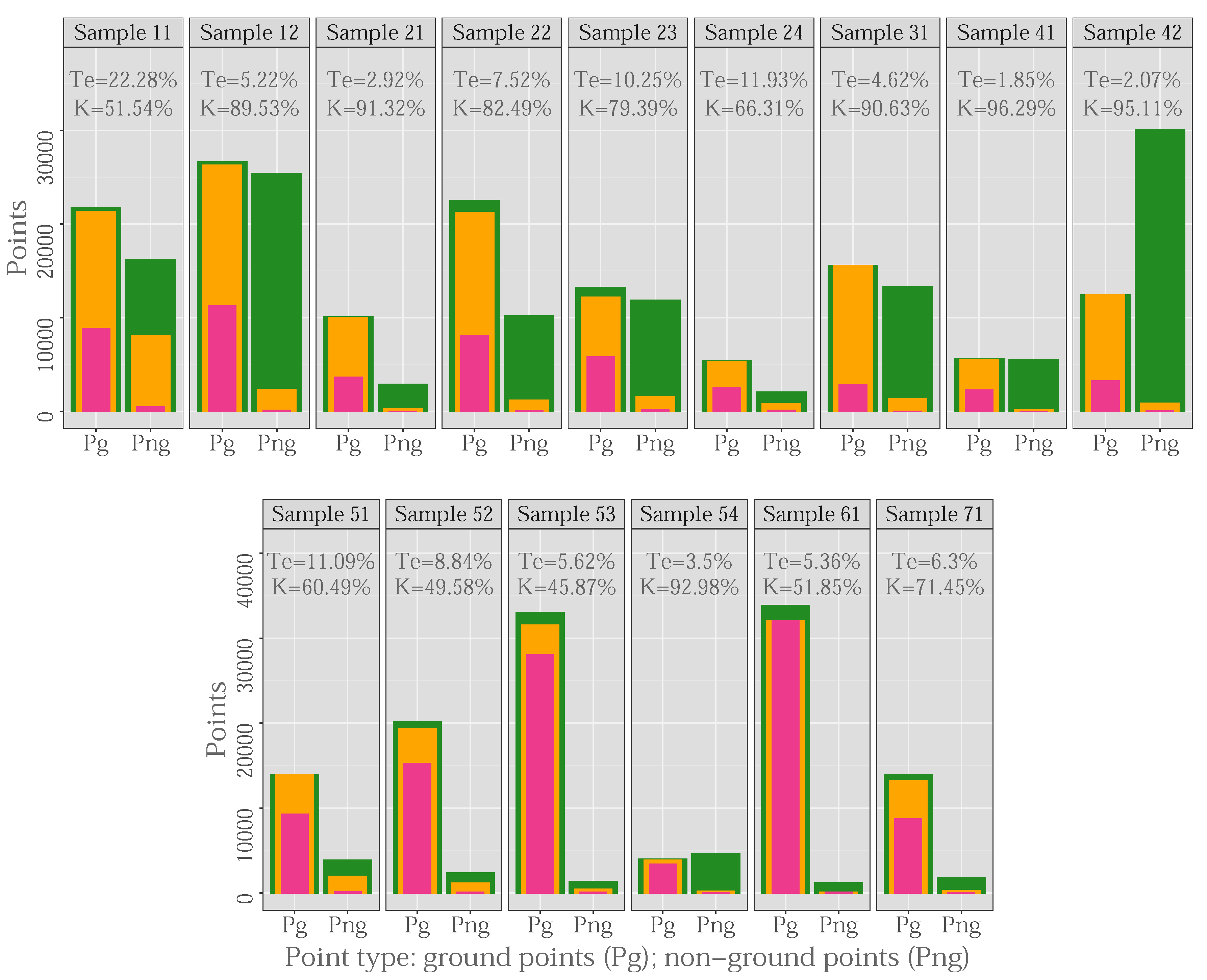
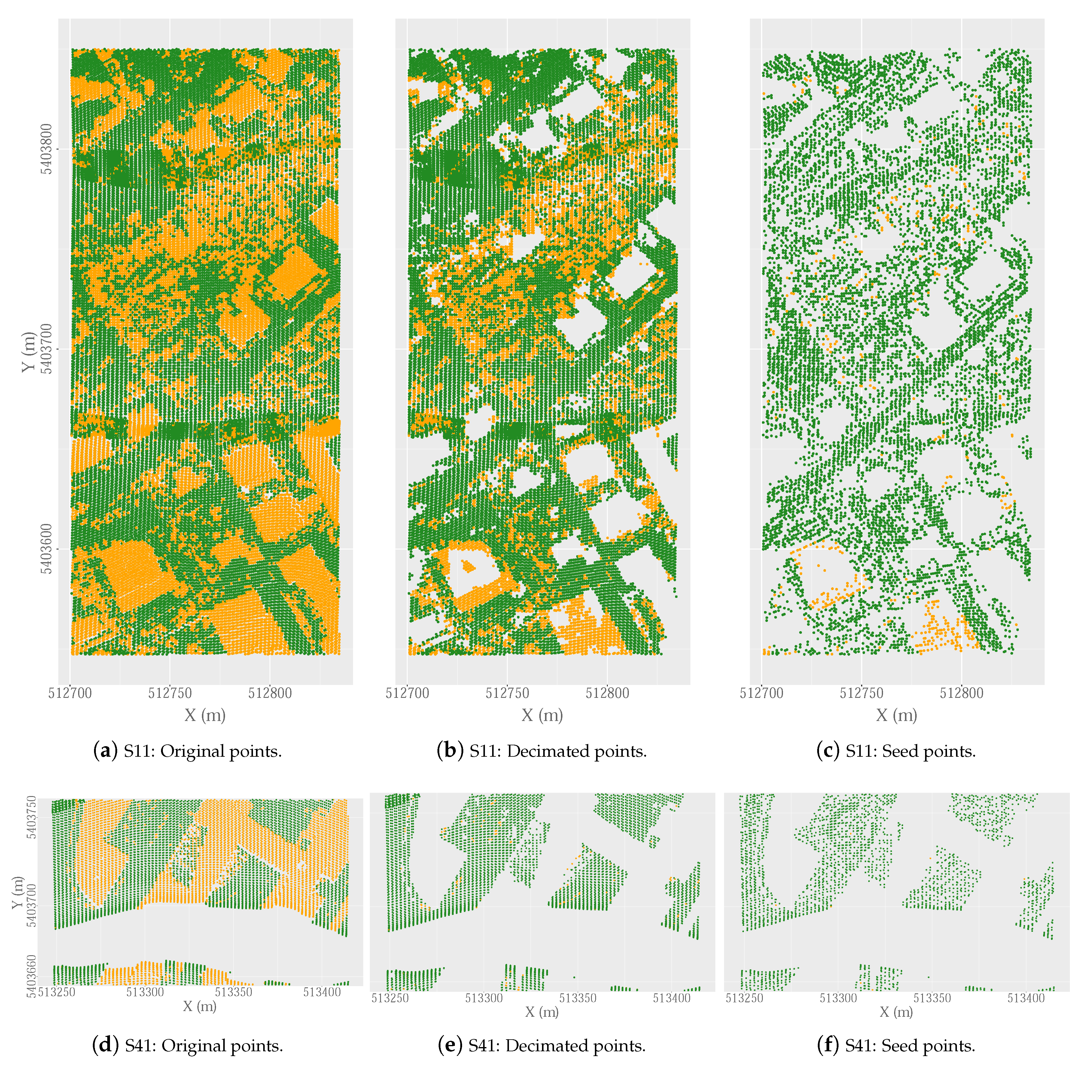
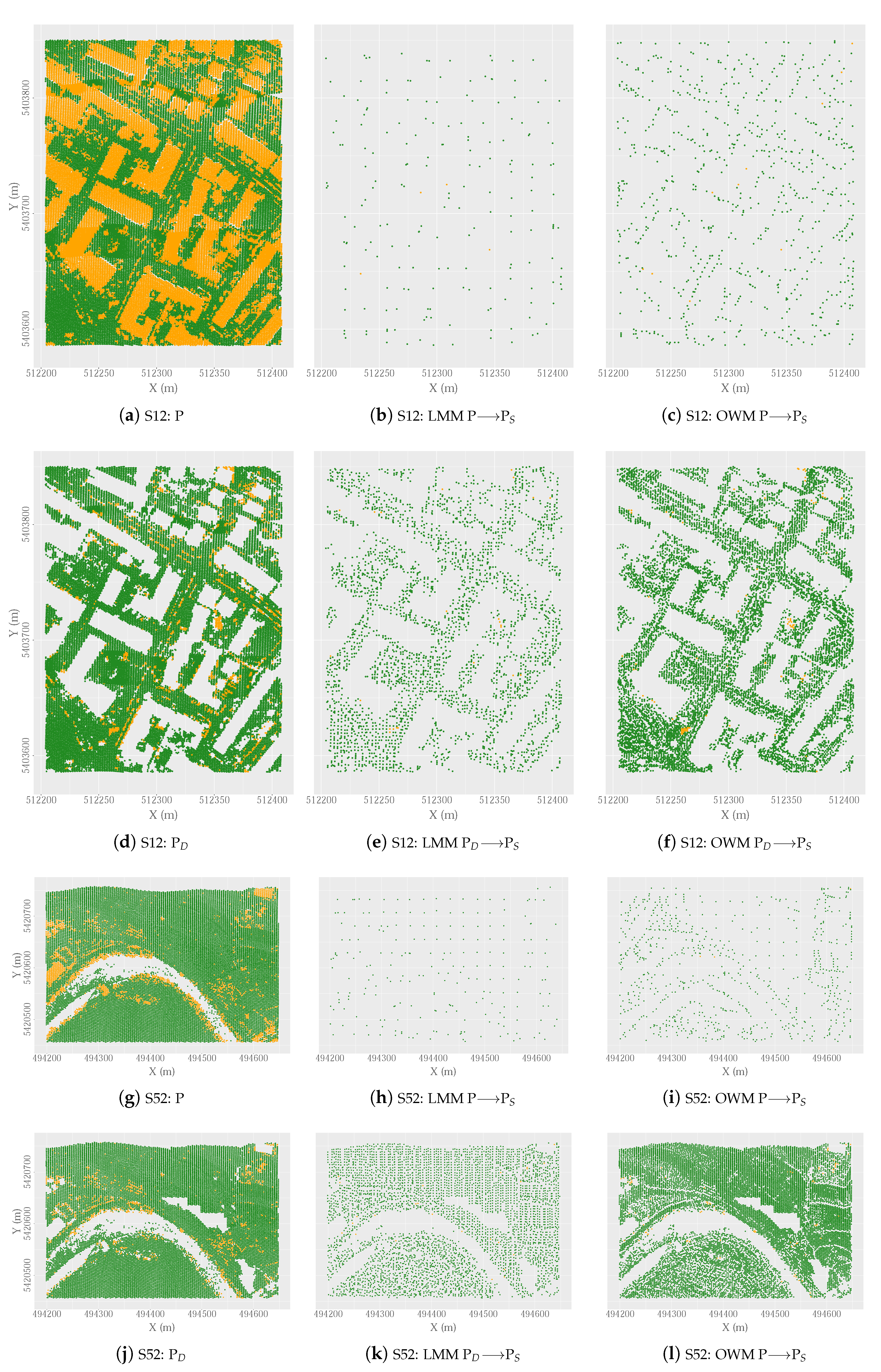
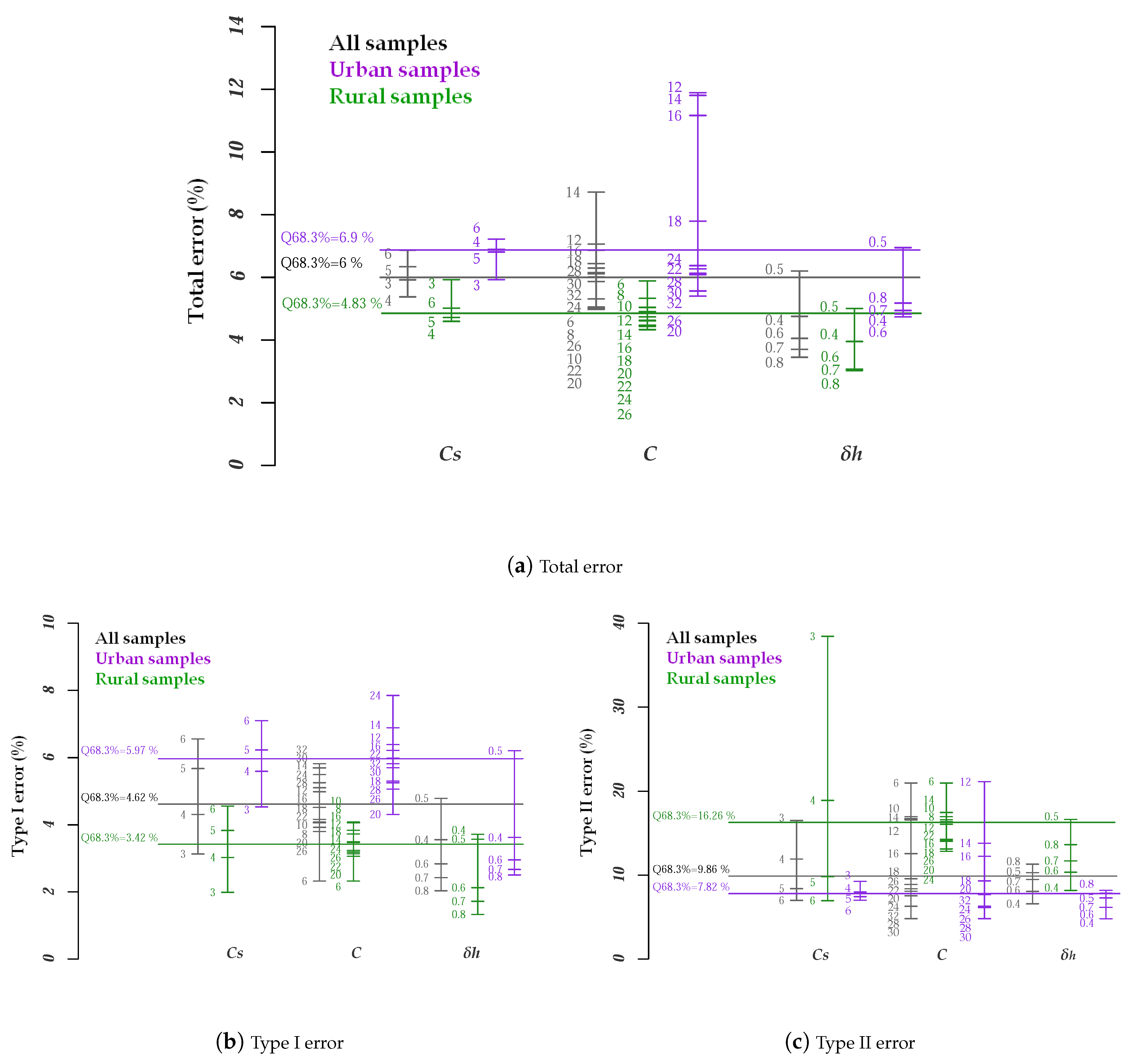
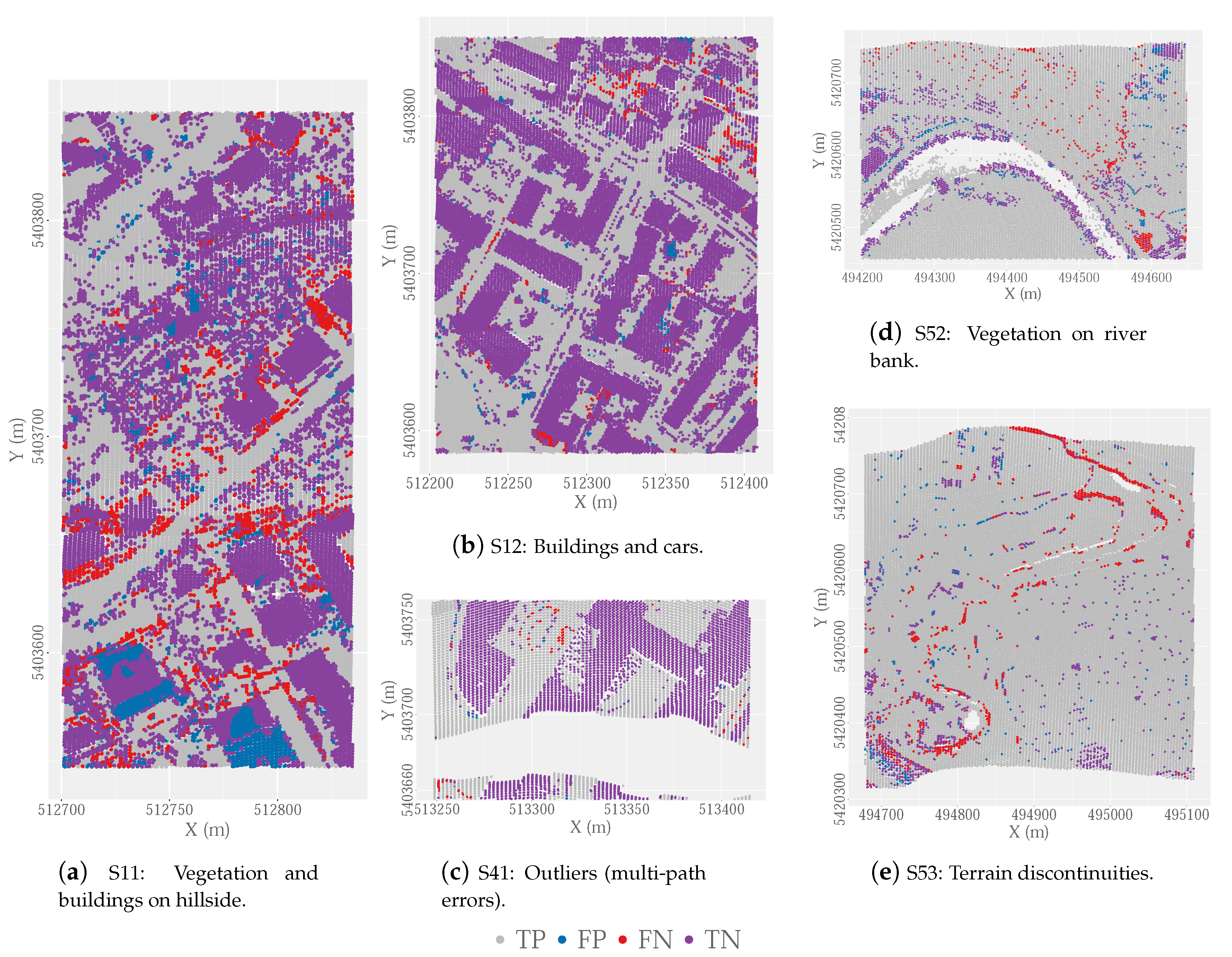
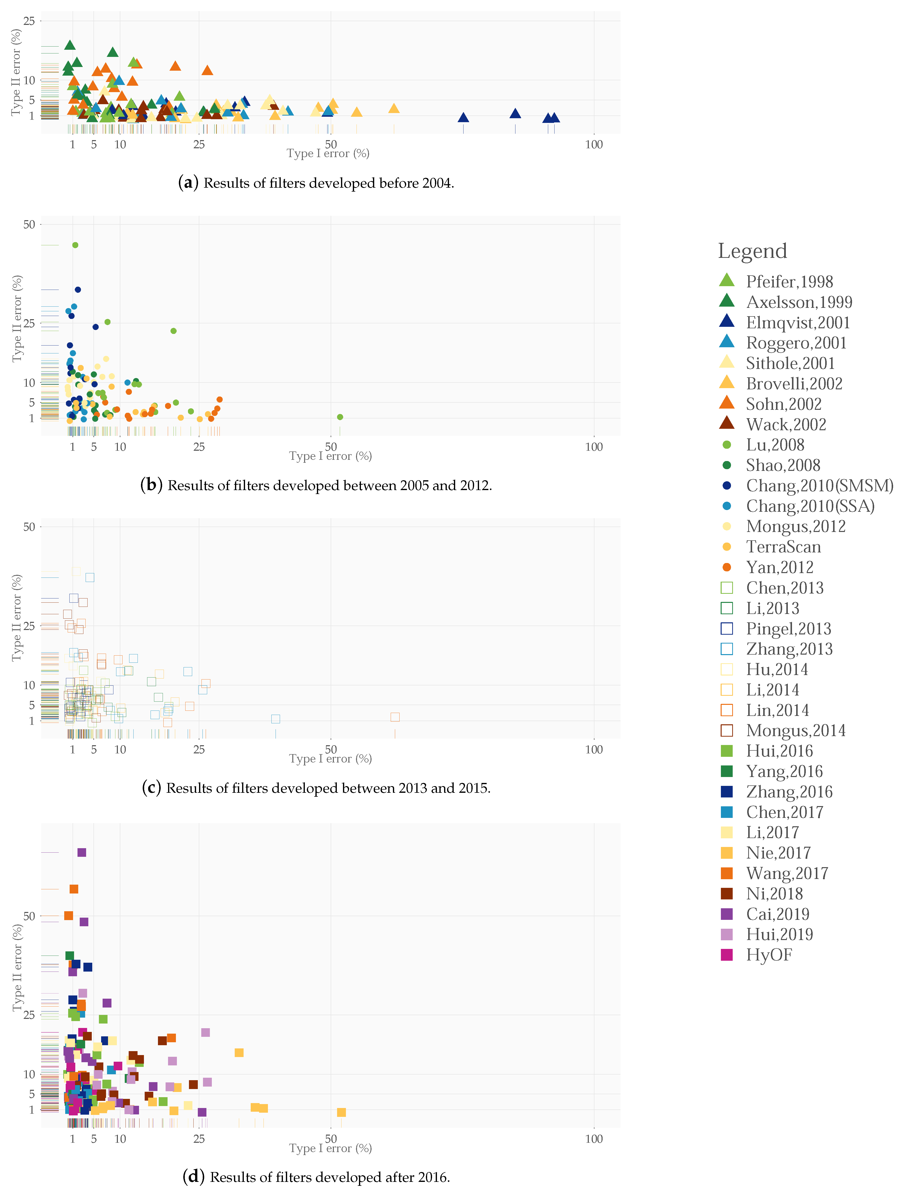
Table 1.
Main limitations of classic filters (source: [20]).
Table 1.
Main limitations of classic filters (source: [20]).
| Main Classic Categories of Filtering Methods | Suitable for | Limitations | Computational Efficiency |
|---|---|---|---|
| Morphology. These methods, based on mathematical morphology, retain terrain details by comparing the elevation of neighboring points. | Terrains with small objects. | • The size and shape of the structuring element. • Forest areas. • Low-density point cloud. • Rough and steep terrains. • Commission errors due to buildings of different heights and complex-shapes. | High |
| Cluster. These methods employ segmentation and clustering techniques to separate terrain points using the point attributes (position, elevation, intensity, etc.). | Urban areas, terrains with various objects. | • Segmentation errors due to the vegetation and complex buildings. • The filtering accuracy depends on the segmentation quality. • Overlapping surfaces (e.g., bridges). • Low-density point clouds make it difficult to find the segment borders. • High-density point cloud ⟶ too many small segments. | – |
| Densification. These methods compare the elevation of points with the estimated values through various interpolation methods (TIN, spline, etc.). In these cases, it is necessary to apply an iterative processing strategy. | Forest areas and steep terrains. | • Dense vegetation or buildings on hillside areas. • Succession of flat and steep areas. • Ramps. • Difficulty in identifying the ground points on breaklines. • Small objects. • Discontinuous terrains. | Middle |
in [21].
Table 2.
Description of the Hybrid Overlap Filter (HyOF) parameters. OWM, Overlap Window Method.
| Fixed | Optimal number of points.np is the mean number of points per cell considered necessary to calculate the penetrability. Default value = 10. |
| Longitudinal and transverse overlap.FO (Forward Overlap) and LO (Lateral Overlap) represent the percentage longitudinal and transverse overlap (expressed as a decimal) between the windows used for selecting the seed points. Default value = 0.8. | |
| Resolution of intermediate raster models.C is the pixel size of the intermediate raster models generated in the densification phase from the points identified as ground points. Default value = 1 m. | |
| Maximum number of iterations.I is the maximum number of repetitions of the densification process. The process will end at the moment at which no new points are classified as ground points or I iterations have been carried out. Default value = 6. | |
| Variable | Maximum size of the area without ground points. C is set on the basis of the length of the shortest side of the largest building in the study area. In forest areas with dense vegetation, where the laser beam does not reach the soil, it is considered to be the maximum distance between any ground point and its nearest neighboring ground point. |
| Size of the window used for selecting the seed points. CS is the size of the moving window used to select the ground seed points. | |
| Residual. is the maximum distance permitted between a point and the reference surface to be considered the ground point. | |
| Automatic | Optimal cell size. CO is the size of the square cell that contains a mean number of np points. It is obtained from the square root of the ratio between np and the weighted mean of point density (D). |
| Minimum and maximum slope threshold. Slmin and Slmax. Some authors [17] use specific percentiles to assign a value automatically to specific parameters during the filtering process, which enables the parameter to be adjusted to the specific characteristics of each study area. In this case, the 65% percentile of the values of the cells of a slope raster () is used to set the value of the parameter Slmin and the 90% percentile to set the parameter Slmax. is calculated from an initial surface () obtained after interpolating a combination of local lowest points. These points are selected with a window size of C by using the OWM function. |
Table 3.
Characteristics of the International Society for Photogrammetry and Remote Sensing (ISPRS) reference samples (Urb.-Urban and Rur.-Rural).
Table 3.
Characteristics of the International Society for Photogrammetry and Remote Sensing (ISPRS) reference samples (Urb.-Urban and Rur.-Rural).
| Samples | Points | Density | Slope (%) | |||
|---|---|---|---|---|---|---|
| Pg(outliers) | Png(outliers) | pts/m | Mean | Q90 | ||
| S11-Urb.Vegetation and buildings on hillside. | 21,786(9) | 16,224 (13) | 1.3 | 0.93 | 53.8 | 100.0 |
| S12-Urb. Buildings and cars. | 26,691 (37) | 25,428 (35) | 1.0 | 0.95 | 11.9 | 26.8 |
| S21-Urb. Narrow bridge. | 10,085 (0) | 2875 (0) | 3.5 | 0.89 | 7.5 | 17.2 |
| S22-Urb. Bridge and gangway. | 22,504 (6) | 10,202 (17) | 2.2 | 0.96 | 16.4 | 43.9 |
| S23-Urb. Large buildings and data gaps. | 13,223 (0) | 11,872 (1) | 1.1 | 0.82 | 24.2 | 60.4 |
| S24-Urb. Ramp. | 5434 (30) | 2059 (1) | 2.6 | 0.83 | 24.1 | 57.0 |
| S31-Urb. Large buildings. | 15,556 (2) | 13,306 (14) | 1.2 | 1.01 | 4.6 | 9.2 |
| S41-Urb. Outliers (multi-path error). | 5602 (0) | 5629 (116) | 1.0 | 0.63 | 12.8 | 28.2 |
| S42-Urb. Railway station. | 12,443 (0) | 30,027 (2) | 0.4 | 0.91 | 6.8 | 15.5 |
| S51-Rur.Vegetation on moderate slopes. | 13,950 (0) | 3895 (0) | 3.6 | 0.18 | 18.9 | 56.2 |
| S52-Rur. Vegetation on river bank. | 20,112 (0) | 2362 (0) | 8.5 | 0.17 | 33.3 | 78.2 |
| S53-Rur. Terrain discontinuities. | 32,989 (0) | 1389 (0) | 23.8 | 0.17 | 39.2 | 78.3 |
| S54-Rur. Low resolution buildings. | 3983 (0) | 4625 (5) | 0.9 | 0.17 | 11.7 | 23.8 |
| S61-Rur. Sharp ridge and embankments. | 33,854 (0) | 1206 (0) | 28.1 | 0.17 | 16.3 | 40.2 |
| S71-Rur. Ramp, bridge, and underpass. | 13,875 (0) | 1770 (0) | 7.8 | 0.18 | 15.0 | 45.4 |
Table 4.
Quantitative results of HyOF obtained by using the ISPRS reference data. The values of the variable parameters in a single combination are C = 4, = 0.5, and C = 30 for urban samples and C = 20 for rural samples.
Table 4.
Quantitative results of HyOF obtained by using the ISPRS reference data. The values of the variable parameters in a single combination are C = 4, = 0.5, and C = 30 for urban samples and C = 20 for rural samples.
| Sample | Optimal Results | Unique Combination Results | ||||||
|---|---|---|---|---|---|---|---|---|
| TIe (%) | TIIe (%) | Te (%) | K (%) | TIe (%) | TIIe (%) | Te (%) | K (%) | |
| S11. Vegetation and buildings on hillside. | 9.59 | 12.06 | 10.64 | 78.27 | 11.76 | 16.90 | 13.95 | 71.44 |
| S12. Buildings and cars. | 2.33 | 2.65 | 2.49 | 95.02 | 3.06 | 3.16 | 3.11 | 93.78 |
| S21. Narrow bridge. | 0.22 | 3.76 | 1.00 | 97.06 | 0.21 | 3.90 | 1.03 | 96.99 |
| S22. Bridge and gangway. | 3.80 | 7.84 | 5.06 | 88.23 | 5.86 | 6.90 | 6.19 | 85.82 |
| S23. Large buildings and data gaps. | 5.49 | 5.86 | 5.67 | 88.64 | 11.16 | 4.30 | 7.91 | 84.19 |
| S24. Ramp. | 2.74 | 9.18 | 4.51 | 88.61 | 5.43 | 7.82 | 6.09 | 85.03 |
| S31. Large buildings. | 0.80 | 1.72 | 1.22 | 97.54 | 0.53 | 2.41 | 1.40 | 97.19 |
| S41. Outliers (multi-path error). | 2.12 | 1.23 | 1.67 | 96.65 | 2.71 | 1.05 | 1.88 | 96.24 |
| S42. Railway station. | 1.10 | 0.69 | 0.81 | 98.05 | 1.10 | 0.69 | 0.81 | 98.05 |
| S51. Vegetation on moderate slope. | 0.47 | 6.42 | 1.77 | 94.72 | 0.18 | 18.95 | 4.28 | 86.59 |
| S52. Vegetation on river bank. | 1.89 | 16.26 | 3.40 | 81.91 | 2.01 | 21.30 | 4.04 | 78.14 |
| S53. Terrain discontinuities. | 2.89 | 20.59 | 3.60 | 62.21 | 4.17 | 17.64 | 4.72 | 56.25 |
| S54. Low resolution buildings. | 1.93 | 2.79 | 2.39 | 95.19 | 1.73 | 4.58 | 3.26 | 93.45 |
| S61. Sharp ridge and embankments. | 0.62 | 11.77 | 1.00 | 85.29 | 3.03 | 2.90 | 3.03 | 67.37 |
| S71. Ramp, bridge, and underpass. | 0.59 | 7.18 | 1.34 | 93.27 | 1.23 | 6.84 | 1.87 | 90.81 |
| All samples | 2.62 | 4.70 | 3.34 | 92.62 | 3.94 | 5.63 | 4.52 | 90.04 |
Table 5.
Comparison of K values obtained in the present study and in 33 previous studies at the sample level.
Table 5.
Comparison of K values obtained in the present study and in 33 previous studies at the sample level.
| Author | S11 | S12 | S21 | S22 | S23 | S24 | S31 | S41 | S42 | S51 | S52 | S53 | S54 | S61 | S71 | K | K | K |
|---|---|---|---|---|---|---|---|---|---|---|---|---|---|---|---|---|---|---|
| Pfeifer (1998) [40] | 66.3 | 91.1 | 92.8 | 85.2 | 83.7 | 79.2 | 96.4 | 78.6 | 93.8 | 89.6 | 41.2 | 31.1 | 90.1 | 47.1 | 66.8 | 83.2 | 86.6 | 62.4 |
| Axelsson (1999) [41] | 78.6 | 93.6 | 86.2 | 91.4 | 92.0 | 88.8 | 90.5 | 72.4 | 96.2 | 91.7 | 83.7 | 39.4 | 70.7 | 74.5 | 91.5 | 89.3 | 90.1 | 78.3 |
| Elmqvist (2001) [42] | 58.9 | 84.2 | 54.9 | 69.3 | 76.6 | 52.1 | 88.7 | 84.8 | 93.6 | 30.1 | 3.3 | 0.6 | 88.9 | 0.7 | 6.9 | 40.9 | 77.8 | 4.8 |
| Roggero (2001) [43] | 59.9 | 86.9 | 75.7 | 54.7 | 54.9 | 54.5 | 95.7 | 75.8 | 89.7 | 91.2 | 60.8 | 25.8 | 50.1 | 21.8 | 78.3 | 73.7 | 75.3 | 54.5 |
| Sithole (2001) [44] | 55.5 | 79.9 | 80.2 | 59.4 | 55.8 | 50.7 | 93.7 | 51.3 | 90.8 | 80.7 | 31.1 | 10.6 | 84.5 | 19.2 | 40.8 | 65.7 | 72.9 | 37.5 |
| Brovelli (2002) [45] | 32.2 | 67.9 | 76.6 | 56.6 | 46.1 | 35.8 | 74.6 | 67.2 | 84.2 | 50.4 | 15.9 | 6.0 | 87.2 | 19.2 | 25.5 | 53.2 | 62.1 | 25.8 |
| Sohn (2002) [46] | 59.5 | 83.2 | 76.1 | 82.3 | 80.2 | 68.6 | 87.1 | 77.6 | 95.7 | 75.5 | 55.0 | 20.3 | 93.5 | 67.5 | 89.1 | 79.8 | 81.6 | 63.3 |
| Wack (2002) [47] | 54.1 | 86.9 | 87.6 | 83.5 | 78.3 | 74.3 | 95.6 | 81.9 | 91.6 | 71.4 | 36.4 | 16.8 | 88.5 | 29.7 | 48.3 | 75.0 | 82.4 | 45.8 |
| Lu (2008) [25] | 43.2 | 80.5 | 69.1 | 72.9 | 78.7 | 64.6 | 89.8 | 73.9 | 88.3 | 82.8 | 57.2 | 17.9 | 86.9 | 46.2 | 62.9 | 75.5 | 75.4 | 58.9 |
| Shao (2008) [12] | 76.0 | 92.0 | 87.2 | 88.6 | 90.4 | 87.7 | 97.6 | 90.1 | 94.8 | 88.9 | 85.6 | 55.0 | 94.5 | 80.7 | 84.7 | 90.5 | 90.1 | 84.7 |
| Shao (2008) [12] | 75.9 | 92.0 | 87.2 | 85.9 | 90.4 | 87.7 | 97.5 | 90.1 | 94.8 | 88.4 | 85.6 | 55.0 | 93.8 | 80.7 | 82.6 | 90.3 | 89.9 | 84.2 |
| Chang (2010) (SMSM) [24] | 72.2 | 93.0 | 96.4 | 93.9 | 91.9 | 84.3 | 97.5 | 85.9 | 96.8 | 90.5 | 79.6 | 60.8 | 94.4 | 82.9 | 89.3 | 91.6 | 91.1 | 87.0 |
| Chang (2010) (SMSM) [24] | 68.9 | 91.2 | 95.3 | 90.9 | 91.9 | 83.9 | 93.4 | 85.0 | 95.0 | 88.2 | 77.5 | 52.2 | 93.5 | 72.4 | 87.7 | 89.2 | 89.1 | 82.1 |
| Chang (2010) (SSA) [24] | 78.1 | 94.3 | 95.0 | 92.2 | 90.6 | 86.7 | 97.9 | 93.9 | 96.6 | 89.3 | 84.9 | 69.5 | 91.4 | 81.0 | 88.2 | 92.6 | 92.2 | 87.8 |
| Mongus (2012) [4] | 77.3 | 89.7 | 94.1 | 84.7 | 88.3 | 80.0 | 93.3 | 92.6 | 87.0 | 92.2 | 68.4 | 42.1 | 86.6 | 65.1 | 85.0 | 87.1 | 87.8 | 76.7 |
| TerraScan | 68.4 | 77.0 | 71.4 | 76.8 | 84.0 | 71.0 | 82.6 | 74.2 | 91.9 | 98.9 | 78.4 | 62.8 | 83.1 | 78.4 | 90.9 | 83.6 | 79.8 | 85.7 |
| Yan (2012) [48] | 62.8 | 86.7 | 82.0 | 75.4 | 68.8 | 55.7 | 92.3 | 71.9 | 87.8 | 81.6 | 57.5 | 24.4 | 84.1 | 33.9 | 52.7 | 76.9 | 79.6 | 56.6 |
| Chen (2013) [29] | 74.1 | 93.2 | 96.1 | 89.0 | 89.5 | 84.5 | 97.8 | 88.8 | 95.8 | 95.2 | 78.9 | 46.7 | 93.8 | 77.4 | 93.2 | 90.5 | 90.5 | 83.4 |
| Li (2013) [49] | 74.3 | 92.5 | 92.8 | 90.6 | 87.7 | 86.1 | 95.0 | 86.6 | 92.8 | 88.5 | 47.1 | 33.1 | 92.1 | 50.0 | 79.2 | 86.2 | 89.4 | 66.6 |
| Pingel (2013) [38] | 83.1 | 94.1 | 96.8 | 92.2 | 90.7 | 91.1 | 98.2 | 88.2 | 96.5 | 95.8 | 81.0 | 68.2 | 95.4 | 87.3 | 91.8 | 93.3 | 92.9 | 90.1 |
| Zhang (2013) [17] | 63.4 | 88.2 | 84.9 | 70.1 | 76.0 | 55.6 | 95.3 | 59.1 | 90.3 | 83.9 | 50.6 | 44.8 | 87.2 | 25.0 | 59.5 | 78.9 | 80.5 | 60.0 |
| Hu (2014) [8] | 83.0 | 94.8 | 97.2 | 92.4 | 91.2 | 90.4 | 98.2 | 88.2 | 98.3 | 93.9 | 86.2 | 66.4 | 95.3 | 86.8 | 92.6 | 93.6 | 93.3 | 89.74 |
| Hu (2014) [8] | 82.8 | 94.0 | 94.3 | 91.8 | 90.5 | 89.5 | 93.4 | 87.5 | 97.1 | 91.5 | 83.7 | 53.1 | 94.6 | 71.1 | 90.5 | 91.7 | 92.1 | 84.1 |
| Li (2014) [50] | 71.8 | 93.5 | 92.7 | 89.7 | 85.3 | 86.6 | 94.9 | 78.5 | 93.6 | 88.6 | 43.6 | 33.7 | 90.7 | 55.6 | 81.3 | 85.8 | 88.7 | 66.6 |
| Lin (2014) [16] | 61.4 | 90.1 | 80.9 | 78.4 | 71.4 | 86.8 | 97.0 | 35.9 | 84.8 | 87.9 | 65.6 | 36.7 | 78.7 | 48.0 | 73.4 | 81.0 | 80.6 | 68.4 |
| Mongus (2014) [51] | 79.0 | 93.4 | 96.0 | 90.1 | 87.6 | 88.8 | 92.9 | 91.9 | 93.2 | 80.1 | 75.6 | 55.6 | 90.8 | 60.1 | 82.5 | 90.0 | 90.6 | 78.8 |
| Hui (2016) [13] | 72.9 | 93.0 | 93.4 | 87.6 | 89.7 | 81.9 | 97.3 | 78.8 | 95.4 | 85.1 | 69.5 | 41.8 | 91.6 | 67.8 | 79.9 | 88.7 | 89.5 | 76.7 |
| Yang (2016) [9] | 78.7 | 94.6 | 91.7 | 89.2 | 91.0 | 91.3 | 96.8 | 95.0 | 97.0 | 88.9 | 84.1 | 66.6 | 93.7 | 81.6 | 70.9 | 92.1 | 92.1 | 85.4 |
| Zhang (2016) [52] | 75.2 | 94.0 | 90.5 | 77.7 | 90.4 | 92.7 | 96.8 | 89.7 | 96.2 | 91.1 | 77.1 | 46.9 | 93.6 | 78.1 | 68.0 | 89.8 | 89.9 | 81.9 |
| Chen (2017) [39] | 80.6 | 94.3 | 96.7 | 91.0 | 91.0 | 90.8 | 97.4 | 92.4 | 98.0 | 94.5 | 83.1 | 62.0 | 94.4 | 85.3 | 90.0 | 93.0 | 92.8 | 88.6 |
| Li (2017) [53] | 74.2 | 92.9 | 94.7 | 91.0 | 89.3 | 85.2 | 91.5 | 75.1 | 85.4 | 86.7 | 67.8 | 38.8 | 89.2 | 73.1 | 86.5 | 87.2 | 87.8 | 75.9 |
| Nie (2017) [54] | 57.8 | 86.9 | 84.1 | 65.5 | 61.6 | 42.7 | 95.6 | 47.7 | 93.1 | 91.8 | 50.8 | 24.0 | 91.8 | 42.8 | 79.9 | 76.3 | 76.6 | 61.8 |
| Wang (2017) [55] | 60.5 | 92.0 | 94.0 | 88.3 | 88.1 | 93.2 | 96.8 | 95.7 | 97.4 | 74.6 | 70.2 | 48.4 | 88.8 | 63.2 | 72.2 | 88.4 | 88.6 | 76.9 |
| Ni (2018) [56] | 63.1 | 82.3 | 79.1 | 69.5 | 79.6 | 58.6 | 85.7 | 88.5 | 87.2 | 93.0 | 54.3 | 31.1 | 89.4 | 61.9 | 73.5 | 79.6 | 79.2 | 69.2 |
| Cai (2019) [37] | 66.0 | 82.3 | 65.2 | 90.0 | 82.8 | 55.3 | 85.5 | 74.1 | 88.4 | 89.1 | 71.9 | 55.8 | 94.8 | 86.9 | 89.3 | 84.5 | 81.7 | 85.2 |
| Hui (2019) [57] | 65.6 | 85.7 | 92.6 | 71.3 | 82.1 | 64.8 | 86.1 | 77.1 | 89.7 | 83.4 | 56.1 | 13.7 | 88.8 | 14.4 | 72.8 | 74.5 | 81.8 | 46.2 |
| HyOF | 78.3 | 95.0 | 97.1 | 88.2 | 88.6 | 88.6 | 97.5 | 96.7 | 98.1 | 94.7 | 81.9 | 62.2 | 95.2 | 85.3 | 93.3 | 92.6 | 92.2 | 88.7 |
| HyOF | 71.4 | 93.8 | 97.0 | 85.8 | 84.2 | 85.0 | 97.2 | 96.2 | 98.1 | 86.6 | 78.1 | 56.3 | 93.5 | 67.4 | 90.8 | 90.1 | 90.0 | 82.4 |
Results obtained using a unique combination of parameters. For HyOF: C = 4, = 0.5, C = 30 for urban samples, and C = 20 for rural samples. in [4]. The best results for each sample.
© 2020 by the authors. Licensee MDPI, Basel, Switzerland. This article is an open access article distributed under the terms and conditions of the Creative Commons Attribution (CC BY) license (http://creativecommons.org/licenses/by/4.0/).
Share and Cite
MDPI and ACS Style
Buján, S.; Cordero, M.; Miranda, D. Hybrid Overlap Filter for LiDAR Point Clouds Using Free Software. Remote Sens. 2020, 12, 1051. https://doi.org/10.3390/rs12071051
AMA Style
Buján S, Cordero M, Miranda D. Hybrid Overlap Filter for LiDAR Point Clouds Using Free Software. Remote Sensing. 2020; 12(7):1051. https://doi.org/10.3390/rs12071051
Chicago/Turabian StyleBuján, Sandra, Miguel Cordero, and David Miranda. 2020. "Hybrid Overlap Filter for LiDAR Point Clouds Using Free Software" Remote Sensing 12, no. 7: 1051. https://doi.org/10.3390/rs12071051
Note that from the first issue of 2016, this journal uses article numbers instead of page numbers. See further details here.