Anomaly Detection for Urban Vehicle GNSS Observation with a Hybrid Machine Learning System
by
 , and
, and
Yan Xia
1,2,3, 
Shuguo Pan
1,2,*,
Xiaolin Meng
3,
Wang Gao
1,2,
Fei Ye
1,2,
Qing Zhao
4 and
Xingwang Zhao
3,5 1
School of Instrument Science and Engineering, Southeast University, Nanjing 210096, China
2
Key Laboratory of Micro-Inertial Instrument and Advanced Navigation Technology, Ministry of Education, Nanjing 210096, China
3
Nottingham Geospatial Institute, The University of Nottingham, Nottingham NG7 2TU, UK
4
School of Transportation, Southeast University, Nanjing 210096, China
5
School of Geodesy and Geomatics, Anhui University of Science and Technology, Huainan 232001, China
*
Author to whom correspondence should be addressed.
Remote Sens. 2020, 12(6), 971; https://doi.org/10.3390/rs12060971
Submission received: 22 February 2020
/
Revised: 14 March 2020
/
Accepted: 15 March 2020
/
Published: 17 March 2020
(This article belongs to the Special Issue Real-time GNSS Precise Positioning Service and its Augmentation Technology)
Abstract
:In urban areas, the accuracy and reliability of global navigation satellite systems (GNSS) vehicle positioning decline due to substantial non-line-of-sight (NLOS) signals and multipath effects. Recently, positioning enhancement approaches with supervised GNSS signal type classification based on 3D building model-aided labelling have received widespread attention. Despite the reduced computing costs and improved real-time performance, the strict requirements of 3D building models on accuracy and timeliness limit the popularization of the technology to some extent. Meanwhile, the diversity of anomalous observation sources is beyond the reach of NLOS/multipath detection methods. This paper attempts to construct an alternative framework for quality identification of GNSS observations combining clustering-based anomaly detection and supervised classification, in which the hierarchical density-based spatial clustering of applications with noise (HDBSCAN) algorithm is used to label the offline dataset as normal and anomalous observations without the aid of 3D building models, and the supervised classifier in the online system learns the classification rule for real-time anomaly detection. The experimental results based on the measured vehicle GPS/BeiDou data show that after excluding anomalous observations the single point positioning accuracy of the offline dataset is improved by 87.0%, 45.9%, and 69.6% in the east, north, and up directions, respectively, and the positioning accuracy of two online datasets is improved by 48.4%/45.7%, 39.6%/63.3%, and 49.6%/49.1% in the three directions. Through a large number of comparative experiments and discussion on key issues, it is certified that the proposed method is highly feasible and has great potential in the practical application of urban GNSS vehicle positioning.
1. Introduction
Global navigation satellite systems (GNSS) robust positioning in urban areas has always been a hot and problematic issue in the navigation field. This is mainly because a large number of multipath and non-line-of-sight (NLOS) effects degrade the positioning performance of a GNSS receiver. Due to the complexity of urban environments, NLOS signal is often more harmful than multipath and its detection and processing are more difficult [1]. With the rise of unmanned technology, intelligent transportation systems (ITS), and smart cities, the demand for accurate and reliable positioning results (including static and dynamic) is becoming more and more urgent. For urban vehicles, a larger positioning error may lead to serious consequences. Especially when vehicles move with little or no human control, the accurate position of the vehicle becomes a vital issue. Meanwhile, the high development cost of autonomous systems makes the GNSS sensor still one of the highest-value components. Proper GNSS NLOS/multipath detection is a critical step for improving vehicle position solutions of both a standalone GNSS system and a multi-source fusion system, and many different methods have been proposed to distinguish between GNSS signal types [2,3,4,5,6]. To avoid the use of specific and expensive hardware, 3D mapping and its derivative methods for dealing with NLOS and multipath have been developed and have shown great potential in urban positioning applications [7,8,9,10]. Their basic principle is to predict satellite visibility by generating building boundaries in the skyplot using a 3D building model. However, it is expensive to establish and maintain accurate 3D building models, and the use of models places high demands on the performance of computing equipment. In recent years, increasingly more scholars have begun to use machine learning or deep learning to identify NLOS/multipath. They attempted to reduce the operating cost of traditional methods and improve usability by constructing a mapping relationship between multiple feature parameters and GNSS signal categories, and achieved good results. In terms of classification algorithms, decision tree [11], support vector machine (SVM) [12,13], convolutional neural network (CNN) [14], and adaptive neural fuzzy inference system (ANFIS) [15] have been successively used for NLOS/multipath recognition. The feature values in most of the above studies are directly or indirectly extracted from the receiver independent exchange (RINEX) format files, which are easy to obtain for GNSS devices. The signal-level feature values are used in [13].
A key issue is that, unfortunately, the classification method based on supervised learning requires the training samples to be labelled in advance, and the labelling accuracy is directly related to the performance of the classifier. As well known, it is always expensive to obtain a labelled dataset that is accurate and can represent all types of states. The current mainstream labelling method is based on the 3D building model, which determines line-of-sight (LOS) and NLOS signals according to the elevation and azimuth angles of the satellite and building boundary [16]. This method is not only limited by the accuracy and timeliness of 3D building models but also requires the accurate position of the receiver to obtain the correct classification label. What is more, in the urban environment, in addition to stationary buildings, there are pedestrians, vehicles, trees, and other factors that interfere with the reception of GNSS signals, which is beyond the application scope of 3D building model. The ray-tracing approach based on the 3D building model can be employed to further determine multipath signals [17,18]. However, this method is computationally expensive and subject to the model accuracy and building materials. This will also lead to another problem, that is, whether the classification model learned from the training set based on certain fixed materials can show sufficient generalization ability when the material of the surrounding obstacles changes as the environment changes. Some other methods for obtaining labels are performed without using the 3D building model. The researchers in [11] utilized the camera, calibrated compass, and accelerometer sensors to calculate the skyline contour. The NLOS and LOS observations were labelled by comparing the elevation and azimuth of the building edge and the satellites. In [14], the authors determined the carrier phase multipath in the real observations based on whether the double-differenced carrier phase residual exceeds three-sigma of measurement errors in a low multipath environment. The process for the former is too complex because of the need for manually labelling. The latter only relies on a single indicator of residuals, which is a rough multipath identification method. The traditional univariate-based method is often suboptimal because when the state is determined by only one variable, it cannot be exactly known, especially in complex urban environments [15]. Therefore, how to accurately label the signal type is a tedious and susceptible process. In addition, except for [14], the other researches only focused on static observation scenarios, which limited the dynamic application of their algorithms in urban areas.
On the other hand, although the large NLOS/multipath error is the most important threat to urban GNSS vehicle positioning, studies focusing on NLOS/multipath detection have not taken into account observation anomaly caused by other factors such as satellite malfunction and receiver fault. Besides, the ranging error caused by NLOS is not always greater than multipath. For some NLOS reflected from close distances, the error is small [19]. There are certain loopholes in simply determining the selection of observations according to the identified NLOS or multipath. In summary, to alleviate the constraints of potential inaccurate signal type labelling on the performance of the classifier, improve the usability and reliability of the classification algorithm, as well as expand the detection object from NLOS/multipath to GNSS anomalous observations, we set our sights on unsupervised anomaly detection (also known as outlier detection) methods and trying to establish observation classification rules that can adapt to multiple urban scenarios. Due to the high complexity of real environments and the diversity of GNSS anomalous observation sources, it is difficult to obtain satisfactory universality of NLOS/multipath detection for both discrimination based on univariate statistical characteristics and supervised classification limited by specific environments and behaviors. Therefore, it may be a better choice to focus on the data itself and mine the distribution patterns of normal and anomalous observations in different contexts. This requires a much larger amount of data. In addition, previous statistical studies on variables related to GNSS signal types provide valuable references for our work [20,21,22,23,24]. Machine learning has the advantage of being able to integrate various information from measurements to improve the accuracy of observation type recognition. The correlation of such measurements themselves and the continuous generation of massive available structured GNSS data from human production activities creates opportunities for unsupervised anomaly detection of GNSS observations.
According to [25], anomaly detection refers to “the problem of finding patterns in data that do not conform to expected behavior”. It is widely applied in various domains, especially financial fraud detection, network intrusion detection, industrial fault detection, and disease detection [26,27,28,29]. Point anomaly (individual anomaly) is the simplest type of anomaly and the focus of most anomaly detection studies. In this article, each GNSS observation can be regarded as a point instance with a specific set of attributes (feature values). When an observation shows an anomalous state with respect to others, it is determined as an anomalous observation. Depending on the availability of labels, anomaly detection can be divided into three modes: supervised, semi-supervised, and unsupervised. Supervised anomaly detection requires the labels for both normal and anomalous classes and semi-supervised anomaly detection requires the labels for only normal class. Unlike them, the unsupervised anomaly detection technique does not need any data label, so it has the most extensive range of application. Nevertheless, it is based on the assumption that normal instances are much more frequent than the anomalous in the dataset, otherwise a high false alarm rate will occur [25]. To fit the assumptions, preliminary screening for offline data can be performed using Chi-square tests in this paper, and the unsupervised anomaly detection algorithm can still work normally as long as the amount of the overall offline data is ensured. There are many kinds of techniques to implement anomaly detection, which are reviewed in detail in some literature [25,30,31,32]. To be specific, an improved clustering-based anomaly detection technique (HDBSCAN) will be used to process offline data for obtaining labels here. It does not need to make any assumptions about the generation distribution of the data and is scalable, with fast feedback on the test set. However, anomaly detection faces one key challenge, that is, it is difficult to characterize normal and anomalous behaviors. In response to this, we plan to make a prior distinction based on the probability distribution of typical characteristic parameters of the dataset, and then use the positioning accuracy after excluding anomalous observations to determine the boundary between the normal and anomalous behavior.
The related studies have inspired us to explore a GNSS observation anomaly detection scheme based on unsupervised learning (clustering), which can effectively identify most of anomalous observations including large NLOS and multipath errors in the urban vehicular context by constructing an appropriate characteristic parameter system and clustering model, without the help of any accurate 3D building model. On this basis, the semi-supervised model or supervised classifier can be used to detect anomalous GNSS observations in real time. The implication of our study is that GNSS observations follow a certain distribution pattern on a multidimensional feature space, and high-quality and available observations generally cluster together, away from anomalous observations caused by diverse interference sources. This paper focuses on the method of vehicle GNSS observation anomaly detection in urban environments, which is a basic and front-end work of GNSS robust positioning, and the purpose of single point positioning (SPP) after excluding anomalous observations is to verify the effect of anomaly detection. Subsequent enhancement methods such as auxiliary measurement information fusion and advanced filtering algorithms are not covered. Our research also provides a new perspective on vehicle GNSS receiver autonomous integrity monitoring (RAIM) in urban environments.
GNSS robust positioning based on 3D mapping is undoubtedly one of the most representative and outstanding techniques for improving urban GNSS positioning accuracy and reliability in the past decade. 3D building model-aided labelling has also been successful in supervised NLOS/multipath detection. The novelty and contribution of this paper is to propose an urban vehicle GNSS anomalous observation detection method mining the data itself when accurate and real-time 3D building models become inaccessible. The structure of the article is as follows: (1) an anomalous observation detection framework based on hybrid machine learning is given first, and the HDBSCAN algorithm is emphasized; (2) the measured vehicle GPS/BeiDou data is used to analyze and verify the innovative method proposed in this paper, and a large number of comparative experiments are conducted; (3) several key issues about the practicality of this method are discussed; (4) the research conclusions and future work are summarized.
2. Methodology
2.1. Feature Extraction
Proper feature values are critical to the performance of machine learning algorithms. In this paper, we refer to the characteristic parameters of NLOS/multipath detection. Previous research has shown that data-level feature values are adequate for NLOS/multipath detection. The features in this article are extracted only from RINEX format files, which contain plenty of useful information about the quality of GNSS observations. By making full use of these feature values combined with reasonable algorithms, it is possible to effectively determine anomalous observations. There has been some literature about the effects of different features on NLOS or multipath detection [11,15,19]. Here, after carefully evaluating most of the above features, eight features are chosen for observation anomaly detection.
Satellite elevation angle: Assigning the weight of each observation based on the satellite elevation angle is the simplest and most common method to reduce the impact of multipath and NLOS signal reception on positioning results. In general, the satellite signal from the higher elevation angle are less likely to be blocked and reflected by a building. However, this is not a universal truth. Affected by the height and distribution of the buildings, high elevation signals may become NLOS, and low elevation signals may become LOS. Nevertheless, the elevation angle is still an important characteristic index to distinguish the NLOS signals.
Carrier-power-to-noise-density ratio (C/N0) measurement: According to the signal propagation theory, additional propagation and reflection will increase the path loss of the GNSS signal. Similar to elevation angle, signal strength or C/N0 has a general correspondence with the type of signal [22]. C/N0 measurement is also a commonly used parameter to mitigate multipath effects. In a complex environment, the contribution of C/N0-based weighting to the positioning accuracy is greater than elevation-based weighting [33]. Multi-frequency C/N0-based multipath detection is implemented by comparing the difference of C/N0 measurements between different frequencies with the value expected for the signal at that elevation angle. However, this indicator is not very suitable for applications where the user moves too fast, such as GNSS vehicle positioning, because the path delay changes with the movement of the receiver antenna, often causing multipath interference to oscillate between constructive and destructive faster than the bandwidth of the C/N0 measurement algorithm [19].
Pseudorange residual: When there are more observation equations than unknown parameters and the position estimates are sufficiently accurate, the magnitude of pseudorange residual can reflect the inconsistency between the pseudorange measurement and the geometric distance. Multi-system fusion positioning increases the number of available observed satellites and observation redundancy. Consequently, pseudorange residual can be used as an indicator to detect GNSS signal quality.
PDOP, HDOP, and VDOP: GNSS positioning accuracy usually depends on dilution of precision (DOP) and measurement error. In the case where the user equivalent ranging error (UERE) is constant, the larger DOP value is, the larger positioning error is. In a dense urban environment, a large DOP value often means a large probability of multipath effect and NLOS reception.
The number of satellites involved in the position solution: The number of available satellites to some extent indicates the quality of the observation environment at the current location, which has a direct impact on the satellite signal quality.
Pseudorange rate consistency: This feature parameter is the difference between delta pseudorange and pseudorange rate, and its mathematical expression is [15]
where delta pseudorange and delta time indicate the change of pseudorange and the time interval between two epochs, respectively. The pseudorange rate is calculated by Doppler shift based on the principle of Doppler effect as
where superscript and subscript denote the index of satellite and frequency; is the carrier wavelength; is the Doppler shift in unit of Hz.
2.2. Hierarchical Density-Based Spatial Clustering of Applications with Noise (HDBSCAN)
HDBSCAN is an improvement based on hierarchical clustering for DBSCAN [34,35]. The principle of the DBSCAN algorithm is that for each cluster, the sample points within a given neighborhood radius must exceed a certain threshold. It is not sensitive to noise and can find clusters of arbitrary shapes [36,37]. However, DBSCAN has two major disadvantages. First of all, it is necessary to manually set the neighborhood radius Eps and the minimum number of samples around the core point MinPts. It is difficult to find appropriate parameters when the spatial density of the samples is uneven, so the parameters may not be universal on different datasets. Secondly, DBSCAN cannot be used for clustering of large-scale data because of the huge computational overhead. HDBSCAN optimizes these problems to reduce the running cost and sensitivity of the algorithm to parameters. What is more, HDBSCAN can handle clustering with different densities. According to the tutorial of the open-source code, the specific implementation steps of HDBSCAN are as follows [38]:
(1) Transform the space according to the density/sparsity. The mutual reachability distance is used to represent the distance between two sample points, so that the distance between the sample points in the sparse area and other points is enlarged, which reduces the dependence of clustering on Eps. The expression of mutual reachability distance is
where is the original metric distance between and ; denotes the distance of nearest neighbor from . Therefore, dense points (with low core distance) remain the same distance from each other, while sparser points are pushed away to be at least away from any other point.
(2) Build the minimum spanning tree of the distance weighted graph. The sample data is treated as a weighted graph, with mutual reachability distance as the weight of the connection edge. A minimal set of edges is found so that removing any edges from the set will split the graph. This minimum set of edges is the minimum spanning tree of the graph, which can be achieved quickly and efficiently with Prim’s algorithm [39].
(3) Construct a cluster hierarchy of connected components. The above minimum spanning tree is converted into the hierarchy of connected components at this stage. The implementation method is to sort the edges of the tree by distance in increasing order, and then traverse to create a new merged cluster for each edge. To obtain a set of flat clusters, we need to know the conditions for terminating the clustering. Therefore, the key to HDBSCAN is how to cut the tree at different places to select the clusters for variable density samples.
(4) Condense the cluster hierarchy based on minimum cluster size. As the most important parameter of HDBSCAN, once MinClusterSize is determined, the minimum spanning tree can be traversed from top to bottom. When each node is split, if the number of sample points of the sub-cluster is less than MinClusterSize, then the samples of this sub-cluster are marked as -1 for “outlier” and deleted. After traversing the entire cluster tree, a new tree with a small number of nodes is finally obtained.
(5) Extract the stable clusters from the condensed tree. Unlike the one-size-fits-all cluster selection method of DBSCAN, HDBSCAN introduces the stability indicator. Here the parameter is defined as the reciprocal of distance. Specifically, there are two measures for a node in the tree and a measure for a point in the node:
- : the lambda value when the cluster is formed
- : the lambda value when the cluster is split into two sub-clusters
- : the lambda value when that point is separated from the cluster
where . For each cluster compute the stability as
The cluster selection follows this principle: if the sum of the stabilities of the sub-clusters is greater than the stability of the cluster, then the cluster stability is set to be the sum of the sub stabilities; otherwise, the cluster is declared as the selected cluster and all its descendants are deleted. When traversing to the root node, the current set of selected clusters is the flat clustering, namely, the final clustering result.
The HDBSCAN class has a large number of parameters that can be set during initialization, but in practice, few parameters have a significant practical impact on clustering. There are mainly two parameters that affect the results of anomaly detection, where MinClusterSize is the minimum size of clusters and MinSamples stands for the number of samples in a neighborhood for a point to be considered a core point. The number of clusters can be reduced by increasing MinClusterSize. The larger MinSamples is, the more points are considered outliers, and clusters will be restricted to more dense areas.
2.3. Hybrid Machine Learning Framework for GNSS Observation Anomaly Detection
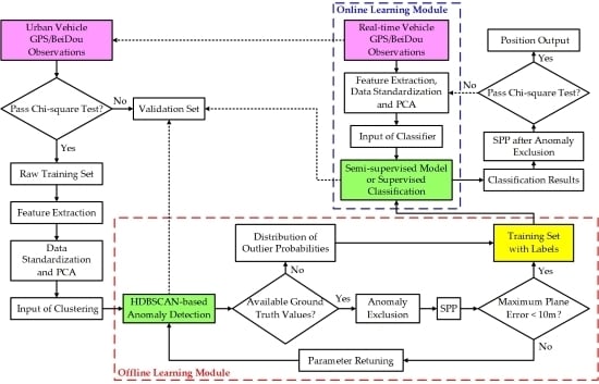
Most individual anomaly detection algorithms, including clustering, are based on post-processing (autonomously learning rules from a large amount of unlabeled sample data), so it is difficult to apply them directly in real time. However, GNSS positioning is more applied in real-time scenarios, especially for vehicle dynamic positioning in the urban environment. To cope with this problem, we designed a real-time detection framework for anomalous GNSS observations, which consists of two major parts, namely an offline learning system and an online learning system. The former provides the latter with prior knowledge of learning. The specific algorithm flow is shown in Figure 1.
In the offline system, considerable urban vehicle GNSS observations are collected, which naturally contains a certain number of anomalous observations. Considering that unsupervised anomaly detection algorithms always work better for the dataset with a small proportion of outliers, we performed a preliminary screening of the original observations based on the Chi-square test. The verification formulas of positioning results are as follows
where is the standard deviation of observation ; is weighted residual; denotes the weighted sum of the squared errors (WSSE) based on residuals; is the number of estimated parameters and is the number of measurements. is Chi-square distribution of the degree of freedom and is false alarm rate. Herein, the value of is set to 0.1% [40]. When meeting the condition, the epoch is marked in the raw training set, otherwise it is assigned to the validation set, which can be verified using HDBSCAN prediction and the online classifier described later. Since the Chi-square test cannot completely exclude anomalous observations, the remaining anomalies help the implementation of the anomaly detection algorithm. After feature extraction and preprocessing, the training set is used as the input for HDBSCAN clustering. There are two ways to determine the ideal anomaly detection results, and the detailed description is given in Section 3.2.1. At this point, the offline labelled database is created. When ground truth values are employed to seek the best parameters here, we can call this process quasi unsupervised learning. Based on the previous research results, when the labels of the training set are accurate enough, the supervised classifiers can always show a good NLOS/multipath recognition performance. This confirms that the accuracy of the prior knowledge and the quality of the training set data are more important than subsequent classification algorithms [41]. Therefore, the establishment of a robust HDBSCAN clustering model for anomalies is the focus of this paper.
In the online system, the semi-supervised model or supervised binary classifier generates classification rules by learning offline labelled data. When the new GNSS observations are input into the classifier, the anomaly detection results can be obtained in real time. Several popular supervised classifiers without parameter fine-tuning are used to verify the system in this article. Finally, like the offline system, we evaluate the effectiveness of anomaly detection with the accuracy and availability of SPP after excluding anomalous observations. Generally, to obtain better real-time positioning accuracy, the Chi-square test can be continued on the final positioning result according to Equation (7). However, the positioning results obtained by the hybrid learning method usually have very few position solutions that fail to pass the verification. When the computing capacity of the device can meet the real-time requirements, for the results that do not pass the Chi-square test, we can update the feature values of their observations and continue to use the online system for further anomaly detection and exclusion. It is generally recommended to iterate only once.
It is worth mentioning that the offline system can learn new HDBSCAN rules and update the labelled database by constantly adding new observations. Training data from more scenarios tend to benefit the performance improvement of the clustering algorithm. Since the exclusion of anomalous observations may cause the number of satellites in the epoch to be too small to calculate position, to facilitate the performance verification of the proposed algorithm, we chose GPS/BeiDou dual-system observations for experiments.
3. Results
3.1. Data Acquisition and Preprocessing
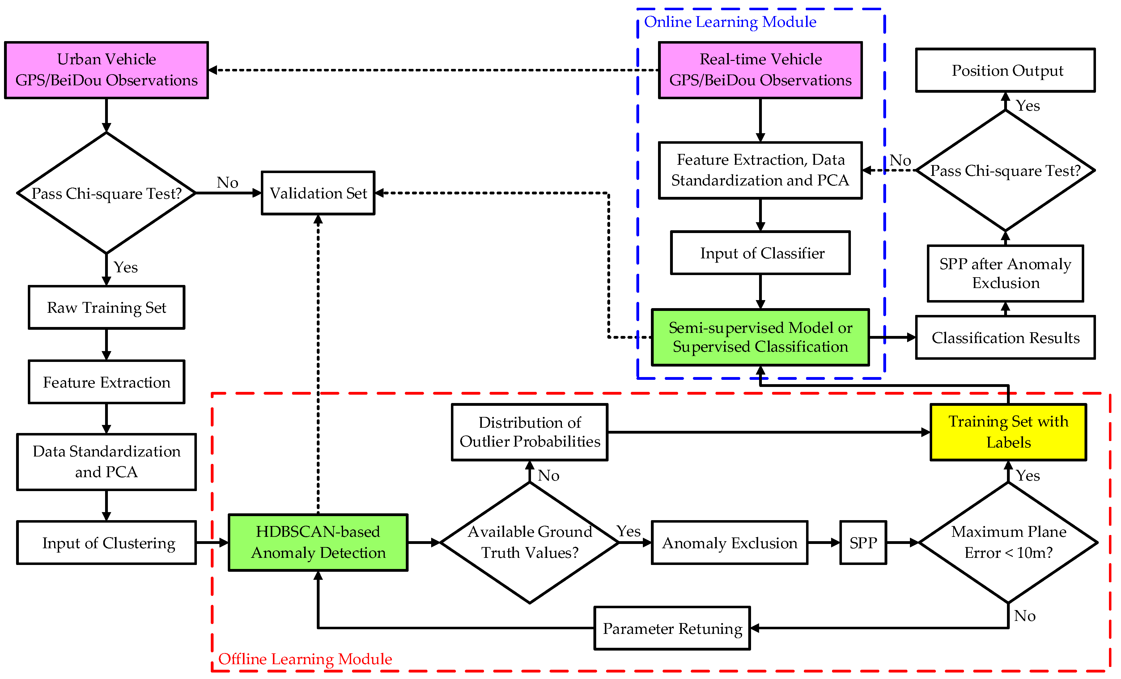
In this paper, we employed vehicle GNSS observations in typical urban environments for experimental verification. The experimental platform and test environment are shown in Figure 2. The external antenna on the roof of the vehicle is connected to different GNSS receivers through a power splitter. Meanwhile, the platform is equipped with a NovAtel’s high-performance tactical grade inertial measurement unit (IMU) ISA-100C for tightly combining GNSS RTK/INS measurements to obtain the calibration values of 3D position, velocity and attitude, which are used to subsequently verify the improvement of positioning accuracy by excluding anomalous observations. The calibration solutions are implemented by post-processing through a high-precision tight combination algorithm from NovAtel Inertial Explorer software. The NovAtel receiver of the rover station and the Trimble receivers of the three base stations contribute the carrier phase observations in tightly combined positioning. It should be noted that due to the heterogeneity between different types of receivers (different hardware configurations and signal processing algorithms), they differ to some extent in terms of satellite signal acquisition and tracking, signal reception strength, observation quality, etc. Therefore, to better demonstrate the universality performance of the proposed algorithm, we leveraged ComNav K508 GNSS OEM board to collect the RINEX data of the training set, while the data collected by NovAtel ProPak6 receiver was used as the test set. Besides, the time interval between the acquisition of the training set and the test set is more than four months. In this case, the spatial-temporal correlation between the datasets will be weakened, which is conducive to a more objective evaluation of algorithm performance.
The average speed of the vehicle was about 30 km/h, and the maximum speed was 50 km/h. In addition to the dynamic observations, the platform also recorded a small amount of static data when stopping at the intersections. The sampling rate of data is 1 Hz. We only process single-frequency observations from GPS L1 and BeiDou B1 bands.
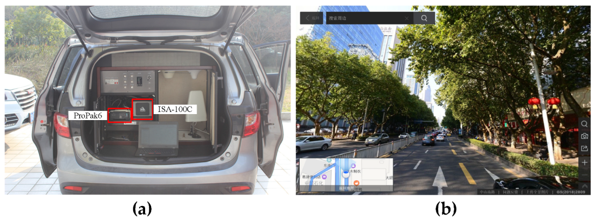
Figure 3 shows the vehicle routes corresponding to three segments of GNSS observations, and the three sets of data are labelled D1, D2, and D3 in chronological order, where D1 is composed of the training set and the validation test, while D2 and D3 are the test sets. Details will be described later. The location where the vehicle travelled is the urban area of Nanjing, and the typical scenarios include urban canyon, semi-urban, tunnel, etc. Many roads in Nanjing are covered by tall London plane trees and other leafy trees. As shown in the figure, D2 and D1 were collected at different places, and the trajectory of D3 had an overlap with D1. Both D2 and D3 are over four months apart with D1.
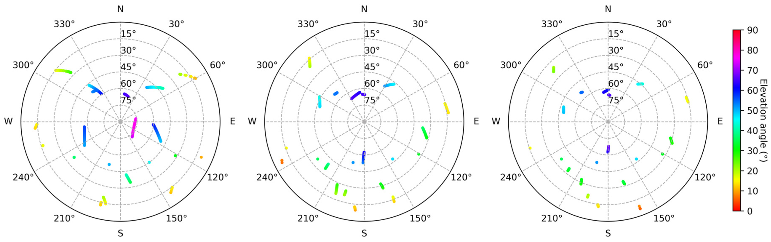
The skyplots of three datasets are also given in Figure 4. Although the path of D3 is included in D1, the satellite distributions of D1 and D3 are still quite different because of unknown changes in the surroundings of overlapping areas and the existence of satellite orbit period. Consequently, there will not be a large number of repeated or extremely approximate feature values between them to affect the reliability verification of the algorithm. Considering the environmental similarity between D3 and D1, we employed D3 as another test set to compare the detection and exclusion effect with D2.
The three sets of data are processed to extract feature values, respectively. In particular, for the integrity of the sample data, we do not set the satellite elevation mask and C/N0 mask during the positioning process, which helps expand the range and diversity of feature values. Details of the datasets are listed in Table 1. The title valid epoch refers to the number of epochs involved in the location resolution. Due to the deterioration of the observation environment, the satellite signal loss of lock will occur, and when the number of visible satellites is less than 5, the dual-system pseudorange single point positioning cannot be performed. These epochs are classified as invalid epochs. Nevertheless, in the urban vehicular environment, there are a considerable number of anomalous GNSS observations at valid epochs. How to effectively identify and eliminate them is exactly what aimed to study in this paper.
We further divide D1 into two parts. The first part contains the epochs in which WSSEs pass the Chi-square test, and the second part is the opposite. As mentioned above, we need to preliminarily screen the training set for more accurate anomaly detection results. The segmented data are shown in Table 2. The subscripts a and b indicate the data of the first part and the second part, respectively. D1a is the training set, and the rest are considered the validation set. In the three datasets, epochs that do not meet the Chi-square test account for 4.4%, 10.0%, and 7.2%, respectively. The observation environment of D2 is worse than the other two. In the traditional RAIM fault detection and exclusion (FDE) algorithm, consistency checking based on the redundancy of range measurements is applied to recovering epochs conflicting the Chi-square test to improve the reliability and availability of positioning results. However, the classical algorithm often fails in urban areas [42]. Therefore, it is also crucial to restore the second part of observations reasonably and effectively, especially for the continuity and integrity of dynamic positioning.
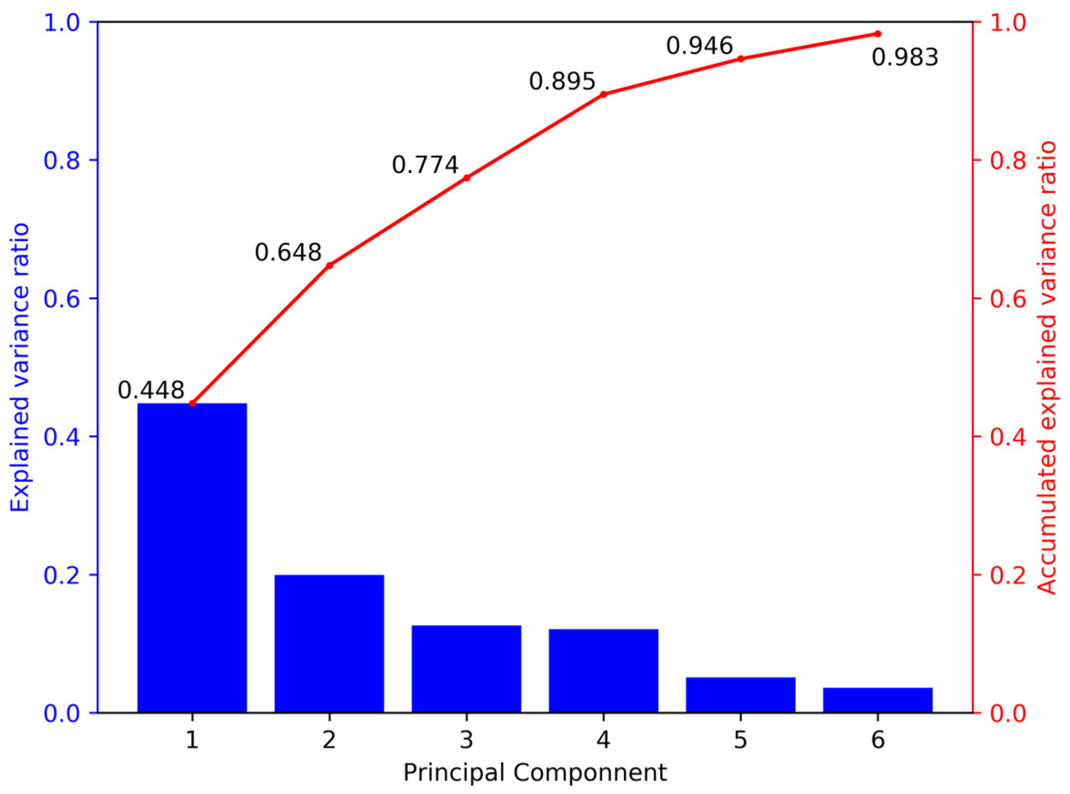
To keep the features of different value ranges at the same numerical magnitude and reduce the influence of the features with large variance on the model, the feature values were standardized so that the mean value is 0 and the variance is 1. On this basis, principal component analysis (PCA) [43] is used to extract key features and improve learning speed. What is more, PCA ensures that these variables are independent of each other to avoid the instability of the solution space. The explained variance ratio represents the contribution proportion of each principal component axis to the variance of the entire dataset. In D1a, for example, the first six principal components cover more than 98% of the training set information, as shown in Figure 5. Therefore, we used these six principal components instead of the original feature values for learning. It should be noted that when testing the algorithm performance with the test sets, the feature values of the test sets must be standardized using the mean and variance parameters calculated by the training test. Similarly, we should use the dimension reduction matrix obtained from the training set to reduce the dimension of the test sets.
3.2. Anomaly Detection Based on HDBSCAN
In this section, we will show in detail the results of detecting anomalous GPS/BeiDou observations on the dataset D1 using HDBSCAN algorithms. This contains a critical post-processing process, which is also the focus of this article, laying the foundation for subsequent supervised learning and real-time applications. At the same time, changes in positioning accuracy and availability after excluding anomalous observations are also analyzed.
3.2.1. Results of D1a
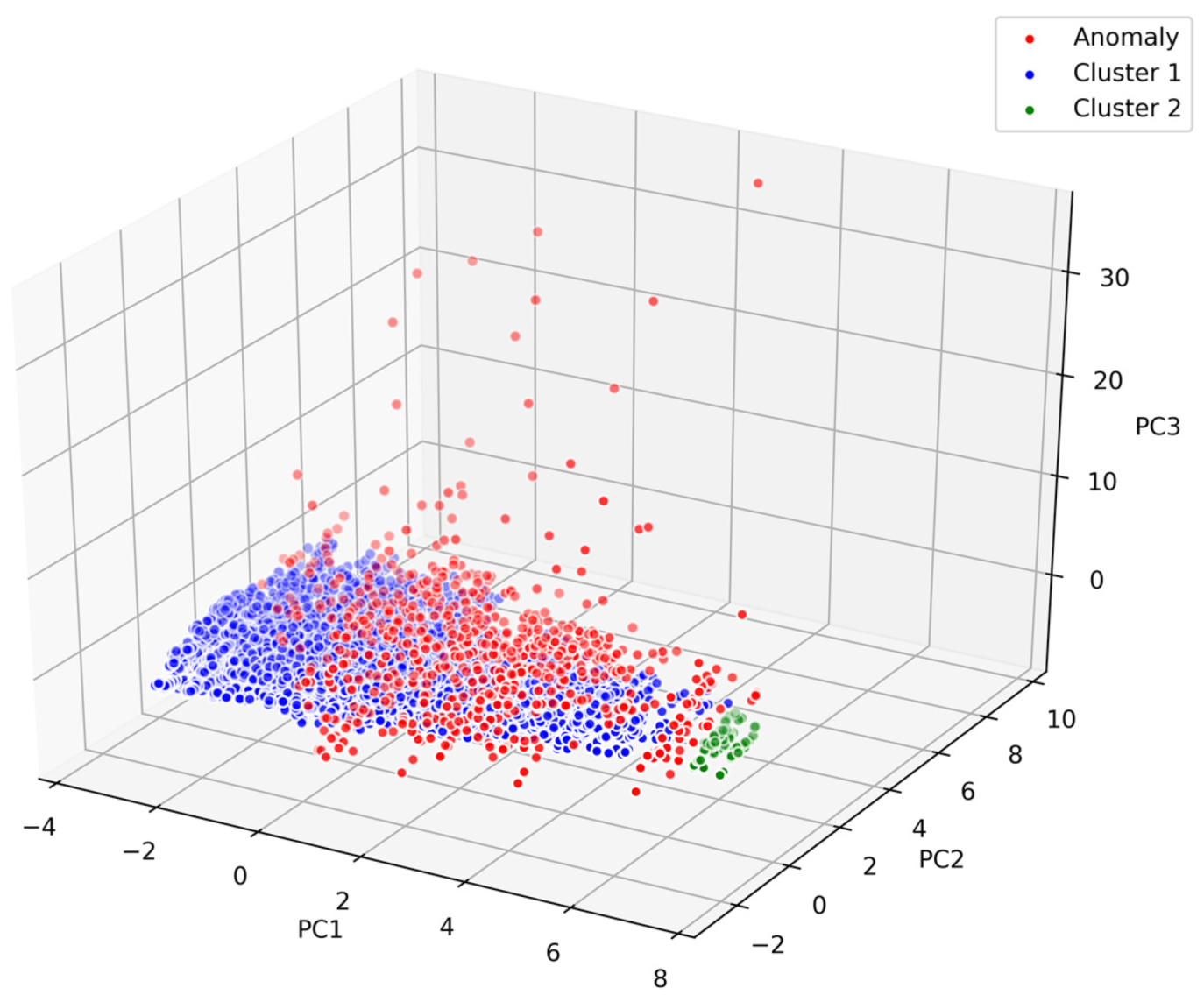
The data subset D1a is first processed using the HDBSCAN algorithm. By parameter tuning, the dataset is grouped into one category as far as possible. The criterion for parameter determination is that as outliers evolve from less to more, the maximum positioning errors in the east and north directions are both less than 10 m for the first time after excluding anomalous observations. This is a relatively conservative approach to reduce false positive rate. Another effective method is to extract the upper quantiles according to the probability distribution of outlier scores in HDBSCAN that describes the possibility of the point becoming an outlier to determine the outlier boundary. In this paper, the maximum positioning error was used to determine the parameters of the clustering model because of the available ground truth values. To be specific, we first fixed MinSamples to the default value and adjusted MinClusterSize. As described in the last paragraph of Section 2.2, the number of clusters can be reduced by increasing MinClusterSize. Therefore, we set the parameter in ascending order. When MinClusterSize is 60, the number of clusters starts to converge to 2 (the rest are outliers), and there are very few sample points in one of the clusters. At this point, we started to adjust MinSamples. The larger MinSamples is, the more points are considered anomalies. To reduce false positive rate, after repeated SPP experiments with anomaly exclusion, we finally set MinSamples to 8, and the results exactly meet the above-mentioned maximum plane error conditions. Figure 6 shows the 3D clustering results when the MinClusterSize is 60 and the MinSamples is 8. For better visualization, the first three principal components (PC) were set as the coordinate axes. It can be seen that the dataset is clustered into two categories, Cluster 1 (blue points) and Cluster 2 (green points), labelled 1 and 0, respectively. Here, the outlier samples labelled -1 are considered “anomalous observations” (red points). However, this is just an intuitive preliminary labelling result, because outliers or anomalies do not necessarily mean anomalous GNSS observations. In some extreme circumstances, anomalous observations in the dataset may behave more like non-outliers than normal observations. Without prior knowledge, there may be a risk that the anomalous observations are wrongly regarded as “normal”, while the normal observations become “anomalous”. Therefore, for the sake of insurance, it is necessary to further confirm the clustering results according to the probability distributions of the feature values.
Figure 7 depicts a pair plot that indicates pairwise relationships between variables in the training set D1a. The subplots on the diagonal axes show the univariate distributions of the corresponding variables. The four variables chosen for illustration are satellite elevation angle, pseudorange residual, C/N0 measurement, and pseudorange rate consistency. According to the probability distributions of the last three variables, it can be determined that the recognition results of anomalous GNSS observations above are generally consistent with prior statistical knowledge. Specifically, the anomalous observations are characterized in probability by the largest absolute pseudorange residual, the lowest C/N0 measurement and the largest magnitude of pseudorange rate difference, which is highly similar to the properties of NLOS signals in the urban environments. Meanwhile, the satellite elevation angle has a weak ability to discern the types of GNSS observations. However, it can still be seen that points with medium-low elevation angles (less than 50°) account for the majority of the anomalies. As for Cluster 1 and Cluster 2, the samples of Cluster 2 are mainly concentrated in the region with higher elevation angle, smaller residual and larger C/N0 measurement. These samples can be defined as high-quality observations, which are most likely derived from completely contamination-free LOS signals under ideal observation conditions. Cluster 1 is a collection of those between high-quality observations and anomalous observations. Due to the interference of low multipath effect or other potential factors, its quality as a whole is not as good as that of Cluster 2, but it can still be used for position solution. In D1, the number of anomalies and non-anomalies is 677 and 18,892, respectively.
Being short of labels, there is no unified evaluation index for clustering results. However, the goal of clustering in this paper is clear, namely, to improve the accuracy and reliability of GNSS positioning in urban environments, so the root mean square error (RMSE) of positioning results after excluding anomalous observations was used as an index to evaluate the performance of clustering. The high-precision RTK/INS tightly combined solution was considered as ground truth values. The single point positioning solutions in this paper were obtained using the weighted least squares (WLS) method based on satellite elevation angle.
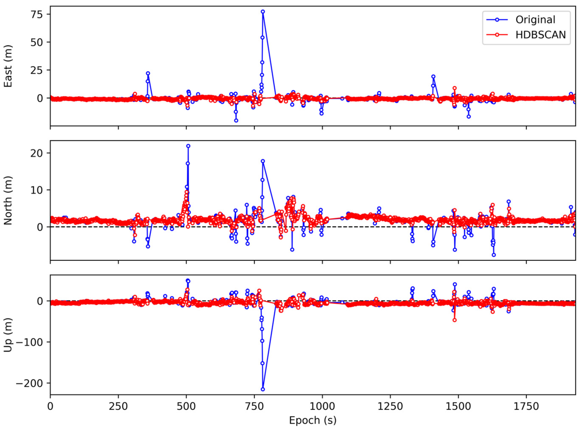
Figure 8 and Table 3 show the improvement in positioning results after HDBSCAN was used to eliminate anomalous observations. The original positioning RMSE without anomaly detection is 3.05, 2.41, and 9.88 m in the east, north, and up directions, respectively. In contrast, the positioning RMSE in the three directions after excluding anomalous observations is 1.09, 2.10, and 6.17 m, with accuracy improvements of 64.3%, 12.9%, and 37.6%. As the vehicle track generally goes from south to north, the positioning error in the east direction is relatively large compared with the north direction [44]. The experimental results show that the removal of anomalies has a better effect on the improvement of positioning accuracy in the east direction, which indicates that HDBSCAN is not only effective to identify GNSS anomalous observations but also consistent with the real situation. The continuity of dynamic positioning results is also of crucial importance while ensuring the positioning accuracy. When there are too few GNSS constellations involved in position solution, it is not advisable to lose a large number of original valid epochs by blindly pursuing the positioning accuracy. In the dataset D1a, the number of valid epochs is 1705, and after excluding anomalous observations the number becomes 1655, making the observed data available up to 97.1%. From Figure 9, besides, as the number of satellites participating in position calculation is reduced due to the exclusion of anomalous observations, the geometric dilution of precision (GDOP) has unsurprisingly risen overall. Even so, the positioning accuracy has been improved. Therefore, this method can effectively identify anomalies in GNSS observations. Moreover, the epochs after using HDBSCAN to remove anomalous observations all meet the Chi-square test.
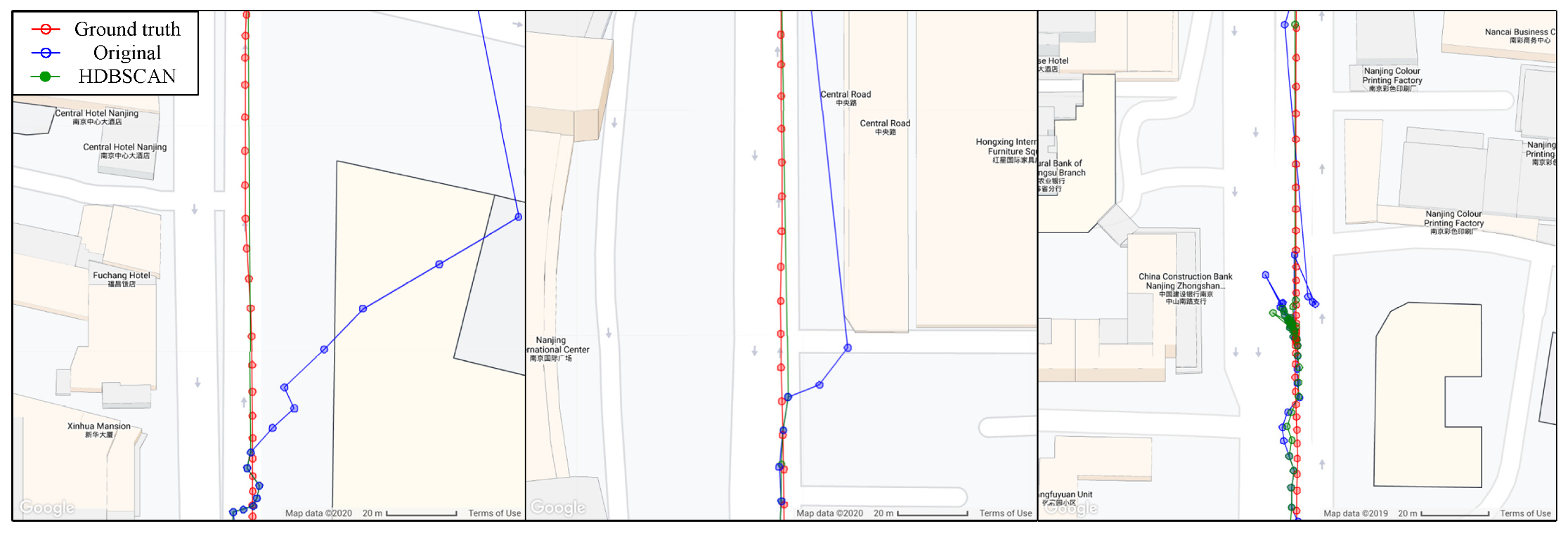
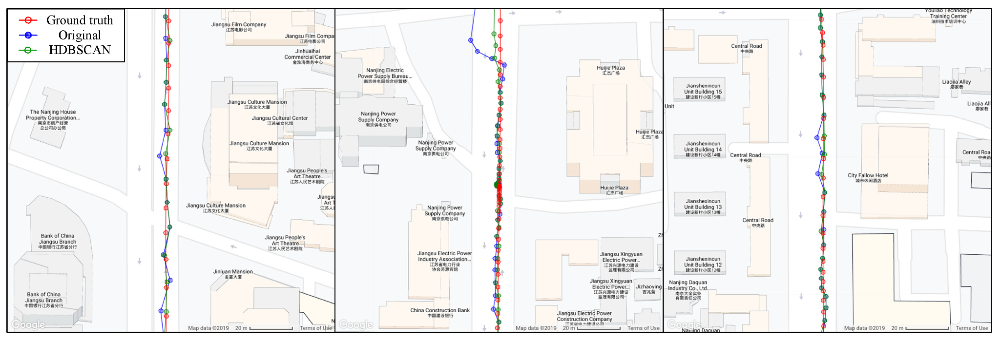
The proposed method can improve the positioning accuracy in two ways. As can be seen from Figure 10, in harsh environments, fewer satellites can be observed and a large number of anomalous observations are mixed into the observation epochs, resulting in huge positioning errors. After anomaly exclusion, there are not enough GPS or BeiDou satellites available for the dual-system positioning process, so these epochs no longer output their positioning results. On the other hand, as shown in Figure 11, when there are sufficient visible satellites and considerable anomalous observations received, the remaining satellites can still participate in the position solution even if the removal of anomalies weakened the satellite geometry, and the positioning accuracy is substantially improved, especially in the east direction. In the former case, some valid epochs are lost due to insufficient normal observations caused by the poor observation environment. However, incorrect coordinate solutions are avoided. Since normal observations are preserved, these epochs can be complemented using their normal observations through advanced filtering algorithms and enhanced information from other sensors or measurements.
In the traditional GNSS single point positioning process, the satellite elevation mask and C/N0 mask are usually set to exclude the observations with poor quality. Therefore, this simple and direct method is also used for comparative experiments. The experimental results are listed in Table 4. When the C/N0 mask is set to 50 dB-Hz, the position solutions of only eight epochs can be obtained, and the availability of high-quality observations is greatly reduced, so this result is ignored. By comparison, it can be found that when the elevation angle mask and C/N0 mask are set to 25° and 0 dB-Hz, respectively, the data subset D1a has the minimum two-dimensional plane positioning error. Nevertheless, the positioning accuracy has not been significantly improved compared with the original result. Some conclusions can be drawn here. Firstly, in urban vehicle-mounted scenarios, the C/N0 measurement has a higher resolution in the positioning results compared with the satellite elevation angle. Specifically, the change of the elevation mask has little influence on the positioning result under the condition of a fixed C/N0 mask until the elevation mask reaches 40°. This also indicates that in the urban environment, the observations are mainly concentrated below the C/N0 measurement of 50dB-Hz and above the elevation of 35°. Secondly, anomalous GNSS observations cannot be effectively eliminated by setting elevation mask and C/N0 mask in a complex urban environment, because the factors affecting the quality of GNSS observations are various. In addition, appropriate cut-off values are not easy to find. If the mask is set too large, the satellite geometric distribution will deteriorate and the number of visible satellites will decrease, thus reducing the positioning accuracy and availability.
3.2.2. Results of D1b
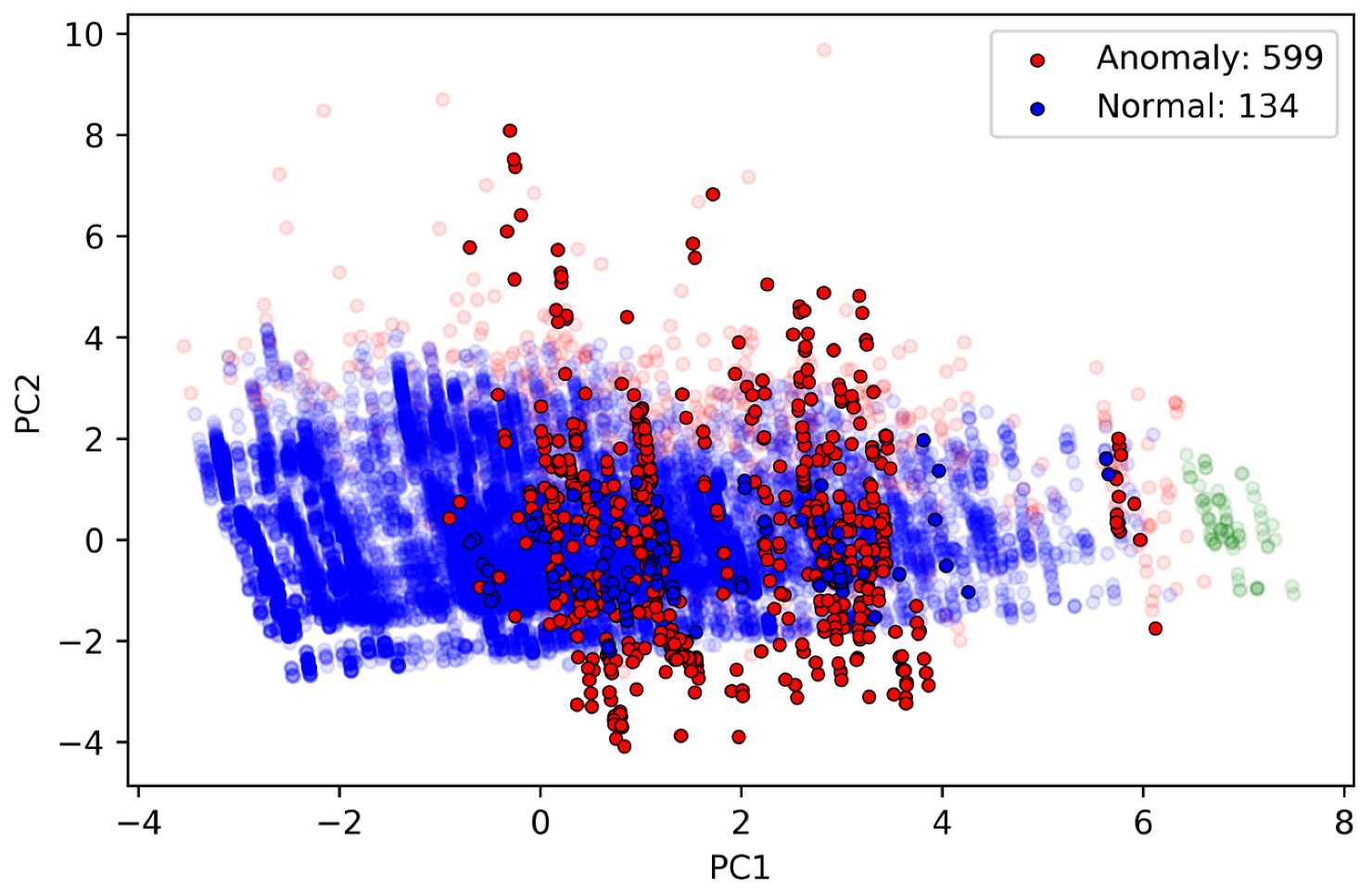
For this part of data, the traditional RAIM FDE algorithm recalculates the position by excluding, one by one, the visible satellites at each epoch. Once meeting the Chi-square test, the position solutions of these epochs are output. However, in epochs with a large number of anomalous observations, the algorithm usually fails. Since HDBSCAN itself can also be used to build predictive models, we first try to predict anomalies of D1b using HDBSCAN which are trained on D1a in this section. The prediction results are shown in Figure 12. To facilitate visualization, the dataset was projected onto the PC1-PC2 plane. There are 599 anomalous observations, obviously more than the normal observations. The remaining 134 normal observations are used for single point positioning to verify the effect of anomaly detection.
Table 5 shows how the above two methods change the positioning results. It can be seen that although RAIM FDE retains most of the epochs, the positioning accuracy does not increase but decreases because the anomalous observations are not effectively eliminated. HDBSCAN improves the plane positioning accuracy to within 1 m, and the two new epochs after excluding anomalous observation meet the Chi-square test. Since the old epochs of D1b do not conform to the Chi-square test, it contains considerable anomalous observations. After identification and elimination of them, the observations that can be used for position calculation will be greatly reduced, so only a small number of epochs are retained. In D1b, although 79 valid epochs contain 134 normal observations, only two epochs with more than five satellites are involved in the solution. This problem will be alleviated once more constellations are introduced.
In addition to the HDBSCAN prediction, we also used some typical supervised classifiers, such as radial basis function (RBF) kernel SVM, decision tree, random forest, adaptive boosting (AdaBoost) and multi-layer perceptron (MLP), to detect anomalous observations of D1b for verification of clustering results. Before the training, we classified Cluster 1 and Cluster 2 in D1a into one category, and anomalous observations into another, forming a binary classifier. The positioning results after classification are listed in Table 6. It can be seen that the positioning results of RBF SVM, decision tree, and MLP are close to that of HDBSCAN. As the availability increases, the positioning accuracy decreases, which indicates that more anomalous observations may be retained in the observations. Therefore, for D1b, both the direct prediction based on HDBSCAN and the classifier based on supervised learning can effectively detect anomalous observations. In addition, to deal with the imbalance of positive and negative samples, an over-sampling method called synthetic minority over-sampling technique (SMOTE) [45] was used to increase the number of anomaly samples. However, the desired results were not achieved.
Similarly, we also set the elevation mask and C/N0 mask for this part of data to compare with the proposed method. The positioning results are shown in Table 7. Obviously, due to the poor quality of the data, the positioning results improve only when the C/N0 mask is set to a large value. One epoch with higher accuracy is retained, which is similar to the results of machine learning methods. However, it is still difficult to determine the optimal elevation and C/N0 mask, which must be consistent with D1a. In practical applications, the cut-off values of the two parts of data are set uniformly. Therefore, it is generally advisable to abandon the recovery of these epochs, so as not to encumber the positioning result of D1a. Combined with the two parts of observations, it is difficult to identify the anomalies by setting the elevation and C/N0 mask in the complex urban vehicle-mounted environment, which has little effect on the improvement of the positioning results.
3.2.3. Overall results of D1
Finally, the overall effect of different anomaly detection and exclusion methods on D1 is listed in Table 8. The best localization performance is achieved by using HDBSCAN-based anomaly detection and exclusion method. Compared with the original positioning results, HDBSCAN improves the accuracy by 87.0%, 45.9%, and 69.6% in the east, north, and up directions, respectively. This is in line with the driving path of D1, and it is clear that more anomalous observations are coming from the cross-street (east) direction. Therefore, after anomaly exclusion, the positioning accuracy in the east direction improves the most. Besides, the availability remains at a high level of 92.9% (of course, it depends on the severity of the observation environment), and all the 1657 epochs meet further Chi-square tests. In complex urban vehicular environments, RAIM and cut-off values cannot effectively improve the positioning accuracy but may cause the accuracy to deteriorate.
3.3. Predicted Results Based on Supervised Classification
The detection results of anomalies on D1a provide a priori knowledge for the supervised classifier in this section. After training the classifier, the predicted results of the new observations can be used for real-time positioning. There are many classification methods based on supervised learning, including complicated deep neural networks with excellent performance. We did not intend to study the network model in depth, because that is not the point of our article. Several typical lightweight classifiers were used to verify the effectiveness and feasibility of the hybrid learning method in GNSS observation anomaly detection. The parameters of each model are only a preliminarily set.
Table 9 and Table 10 list the positioning results of D2 and D3 using different anomaly detection and exclusion methods, respectively. The figures in parentheses represent the number of epochs that do not conform to the Chi-square test. Overall, the RBF SVM classifier has the best effect on the improvement of location results. In D2, the positioning accuracy is improved by 48.4%, 39.6%, and 49.6% in the three directions. The availability is 75.6% because of the harsher environment than D1. While in D3, the positioning accuracy is improved by 45.7%, 63.3%, and 49.1%, and the availability remains at 87.8%. The positioning accuracy improvement of D3 is slightly greater than that of D2, which may be caused by the overlap between the observed trajectories of D3 and D1. Moreover, the positioning accuracy improvement of MLP for D3 is comparable to SVM, which indicates that SVM is not necessarily the only suitable classifier. Better results are expected through more refined parameter tuning. It can be seen that after the anomaly detection and exclusion with the proposed method, the epochs composed of the remaining observations basically conform to the Chi-square test, which also shows the reliability of the algorithm from another perspective.
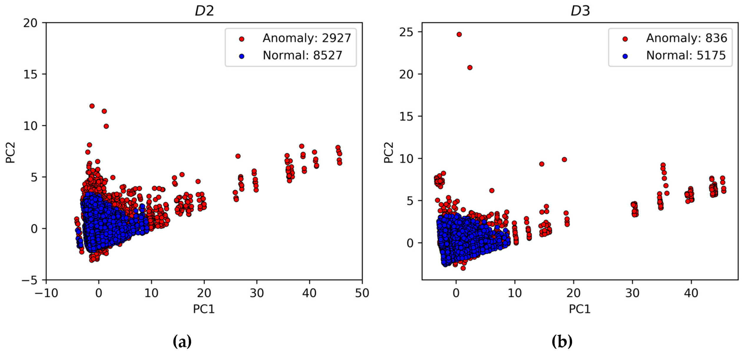
Figure 13 shows the predicted anomaly results of D2 and D3 on the PC1-PC2 plane using RBF SVM. The subgraph of D2 is zoomed in because some anomalies deviate too far from the normal. After processing by the classifier, normal observations are clustered together, while anomalies are scattered everywhere, which conforms to the assumption from the first category of clustering-based techniques in [25]. Intuitively, the results of the classification are also credible. Nevertheless, the incomplete feature values from the training set and the less elaborate classification model will result in a certain amount of false and missed detections. In addition, the number of satellites and DOP values will drop after excluding anomalous observations, so there may be a small number of relatively large errors in the positioning results, which does not affect the improvement of the overall positioning performance.
In general, the classifier performs better on the training set than on the test set. Although satisfactory anomaly detection results of the above test sets are obtained by using the hybrid learning rule, the generalization ability of the classification model can still be improved through the following points. Firstly, longer observations from more scenarios should be collected to increase the number of samples in the training set and avoid overfitting. Secondly, it is necessary to extract better and more descriptive feature values, which are not limited to RINEX-level measurements. Finally, the best performance is achieved by selecting a more appropriate classifier and fully tuning the parameters of the model.
4. Discussion
4.1. The Necessity of Chi-Square Test Separation
As mentioned above, HDBSCAN-based anomaly detection makes the implicit assumption that anomaly points in the sample set account for a small proportion. Therefore, before the clustering algorithm started to run, the Chi-square test is used to separate the offline dataset, where observations in epochs that meet the Chi-square test are considered as the raw training set. To verify the significance of this step, we also used HDBSCAN directly on the whole dataset without Chi-square test separation for the comparative experiment. The parameter determination method is the same as described in Section 3.2.1. Unfortunately, with more anomalies in the dataset, parameter tuning becomes a challenge. When the availability of the dataset without separation is less than 1657 epochs, its positioning error still exceeds the dataset with Chi-square test separation. Additionally, it has five epochs that do not meet the second Chi-square test, as shown in Table 11. During the parameter tuning process, as more “outliers” are detected, the positioning accuracy becomes higher, but the availability will drop sharply, which is not desirable. Through the comparative experiment, it can be found that excessive outliers affect the performance of HDBSCAN anomaly detection and may cause a high false alarm rate, that is, some normal observations are considered as anomalies. Of course, there are many methods of preliminary screening for the dataset, among which the Chi-square test is only a representative one. Besides, the different values of also affect the screening results. However, when clustering-based anomaly detection is performed, reducing the ratio of anomalous observations is a critical step.
4.2. The Balance between Accuracy and Availability
Due to the lack of true and accurate anomaly labels, we can only verify the effectiveness of the anomaly detection algorithm and supervised classifier by the accuracy of the positioning results after excluding anomalous observations, while also taking into account the availability. However, directly deleting anomalous observations reduces the number of available satellites and weakens the geometric distribution, which also affects the positioning performance to a certain extent. For dual-system GNSS positioning, when the number of satellites is less than five, the positioning process cannot be performed. While correct anomaly detection and exclusion can greatly improve positioning results, it must be acknowledged that this improvement is limited by the above disadvantages in areas where only a few satellites are available. Some epochs cannot output the position due to the too few satellites available, and some epochs can only obtain the suboptimal accuracy due to the poor geometric distribution. Suggestions about determining whether to include, exclude, or downweight multipath or NLOS observations within the navigation solution are given in [19]. In addition, the measurement information from external sensors can also be used to enhance the availability and positioning accuracy of GNSS observations. Although no forthcoming well-developed methods or techniques are available for autonomous integrity monitoring based on standalone GNSS receivers, the integrity monitoring approaches without any additional sensors are considered more promising and attractive because they can reduce the complexity and cost of the on-board equipment [42]. It is certain that when there are sufficient GNSS constellations available, the room for optimizing signal selection will be larger. For D1, a total of 127 epochs have to be abandoned due to fewer than five satellites.
4.3. Performance of RAIM with Different False Alarm Rates
In traditional RAIM, Chi-square test based on WSSE is a commonly used method. However, it can only determine whether the measured values are consistent or not, and cannot pick out which observations are anomalous. The epochs that do not meet the Chi-square test are directly discarded, which causes a huge waste of observation information. The positioning error at the epoch conforming to the Chi-square test is still likely to be large because the anomalies cannot be detected completely. In addition, how to properly determine according to the severity of the environment is also a difficult problem. A large value of indicates strict inspection conditions, but it also means a large false alarm rate and low credibility. To make our argumentation more complete, a batch of positioning experiments by setting different values are conducted, and the critical values are obtained by looking up the Chi-square distribution table. The positioning results are listed in Table 12. It can be seen that as the value of increases, the positioning accuracy becomes higher. However, again, when the availability of RAIM is less than 1657 epochs (the confidence is only 0.3), its plane positioning error is still larger than the proposed method. RAIM improves the overall positioning accuracy by discarding the low-precision positioning results it considers, but for other position solutions, it does not improve the accuracy but maintains their original state. On the other hand, as described in Section 3.1, the overall observation environment of D1 is not very severe, resulting in high availability of RAIM. Although the two schemes are not very comparable (one for epochs and one for observations), we still have a reason to believe that when the available constellations increase or the environment is worse, the superiority of the proposed method will be better demonstrated. As can be seen from the results of the last row in the table, RAIM FDE almost completely fails in urban vehicular environments, regardless of the false alarm rate, while RAIM alone cannot recover abandoned epochs. The authors have thoroughly discussed the limitations of classic RAIM in urban environments in their review article [42], including the difficulty in establishing error statistical models, the reduction of available observations, the existence of a large number of NLOS, and the criteria for integrity risk. Besides, the existing RAIM algorithm in the urban environment needs to be further improved.
5. Conclusions and Future Work
With the continuous development of ITS and autonomous driving, vehicles require significantly improved accuracy and reliability in terms of communication, time, and position awareness. However, the deterioration of GNSS observation quality caused by the complexity of the urban environment has become one major challenge for reliable positioning, navigation, and timing (PNT) technology. This paper proposed an anomaly detection frame for urban vehicle GNSS observations, consisting of an offline learning system and an online learning system. In the offline system, HDBSCAN clustering is used to detect anomalous observations and construct the labelled offline training set without the need for 3D building models. On this basis, a supervised binary classifier in the online system acquires the classification rule by training the labelled datasets, which are used for anomaly detection of vehicle GNSS observations in real time. The algorithm was validated with measured GPS/BeiDou single frequency data collected by different types of receivers. HDBSCAN-based anomalous observation detection and exclusion improve the original SPP accuracy of D1 by 87.0%, 45.9%, and 69.6% in the east, north, and up directions, respectively. After using the unrefined RBF SVM classifier to detect and exclude anomalies on D2/D3, the positioning accuracy is improved by 48.4%/45.7%, 39.6%/63.3%, and 49.6%/49.1% in the three directions. Besides, the article gave a lot of comparative experiments, including RAIM (FDE), elevation angle and C/N0 cut-off values, different classification methods, etc. At the same time, some key issues in the practical application of the proposed method were discussed in depth. As the results show, this scheme can greatly improve the positioning accuracy in the urban vehicular environment and has good retention of the availability of observations.
As an exploratory work, the main contribution of this research is to propose a clustering-based anomaly detection method for urban vehicle GNSS observations and demonstrate its feasibility in detail. In the follow-up work, we will further improve it in the following aspects. Firstly, more GNSS observations will be used to establish the offline labelled dataset, so that the training set can cover more scenarios, and increase the generalization ability of the classification model. Secondly, it is necessary to conduct in-depth research on the feature parameters for the types of constellations due to the differences between GNSS constellations. Finally, more suitable anomalous observation detection methods will be sought based on different assumptions for anomaly distribution.
Author Contributions
Conceptualization, Y.X. and W.G.; methodology, Y.X.; formal analysis, Y.X. and Q.Z.; data curation, F.Y.; writing—original draft preparation, Y.X.; writing—review and editing, X.M. and X.Z.; supervision, S.P. and X.M. All authors have read and agreed to the published version of the manuscript.
Funding
This research was funded by the National Natural Science Foundation of China (41774027), the National Key Research and Development Program (2016YFB0502101), the Jiangsu Graduate Research Innovation Program (KYCX19_0067) and the National Natural Science Foundation of China (41704008).
Acknowledgments
The authors would like to thank the anonymous reviewers for their constructive and valuable suggestions on the earlier drafts of this manuscript.
Conflicts of Interest
The authors declare no conflict of interest.
References
- Groves, P.D.; Jiang, Z.; Wang, L.; Ziebart, M.K. Intelligent Urban Positioning using Multi-Constellation GNSS with 3D Mapping and NLOS Signal Detection. In Proceedings of the 25th International Technical Meeting of the Satellite Division of the Institute of Navigation (Ion Gnss 2012), Nashville, TN, USA, 17–21 September 2012. [Google Scholar]
- Petovello, M.; O’Driscoll, C.; Lachapelle, G. Weak signal carrier tracking of weak using coherent integration with an ultra-tight GNSS/IMU receiver. In Proceedings of the European Navigation Conference, Toulouse, Lauragais, France, 23–25 April 2008. [Google Scholar]
- Soloviev, A.; Van Graas, F. Use of deeply integrated GPS/INS architecture and laser scanners for the identification of multipath reflections in urban environments. IEEE J. Sel. Top. Signal Process. 2009, 3, 786–797. [Google Scholar] [CrossRef]
- Jiang, Z.; Groves, P.D.; Ochieng, W.Y.; Feng, S.; Milner, C.D.; Mattos, P.G. Multi-constellation GNSS multipath mitigation using consistency checking. In Proceedings of the 24th International Technical Meeting of the Satellite Division of the Institute of Navigation (ION GNSS 2011), Portland, OR, USA, 19–23 September 2011; pp. 3889–3902. [Google Scholar]
- Jiang, Z.; Groves, P.D. NLOS GPS Signal Detection Using a Dual-polarisation Antenna. GPS Solut. 2014, 18, 15–26. [Google Scholar] [CrossRef] [Green Version]
- Sánchez, J.S.; Gerhmann, A.; Thevenon, P.; Brocard, P.; Afia, A.B.; Julien, O. Use of a fisheye camera for GNSS NLOS exclusion and characterization in urban environments. In Proceedings of the 2016 International Technical Meeting of The Institute of Navigation, Monterey, CA, USA, 25–28 January 2016; pp. 283–292. [Google Scholar]
- Groves, P.D. Shadow matching: A new gnss positioning technique for urban canyons. J. Navig. 2011, 64, 417–430. [Google Scholar] [CrossRef]
- Peyraud, S.; Bétaille, D.; Renault, S.; Ortiz, M.; Mougel, F.; Meizel, D.; Peyret, F. About Non-Line-Of-Sight Satellite Detection and Exclusion in a 3D Map-Aided Localization Algorithm. Sensors 2013, 13, 829–847. [Google Scholar] [CrossRef] [Green Version]
- Hsu, L.-T.; Gu, Y.; Kamijo, S. 3D Building model-based pedestrian positioning method using GPS/GLONASS/QZSS and its reliability calculation. GPS Solut. 2015, 20, 413–428. [Google Scholar] [CrossRef]
- Miura, S.; Hsu, L.-T.; Chen, F.; Kamijo, S. GPS Error Correction with Pseudorange Evaluation Using Three-Dimensional Maps. IEEE Trans. Intell. Transp. Syst. 2015, 16, 3104–3115. [Google Scholar] [CrossRef]
- Yozevitch, R.; Moshe, B.B.; Weissman, A. A robust GNSS LOS NLOS signal classifier. Navigation 2016, 63, 429–442. [Google Scholar] [CrossRef]
- Hsu, L.-T. GNSS multipath detection using a machine learning approach. In Proceedings of the 2017 IEEE 20th International Conference on Intelligent Transportation Systems (ITSC), Yokohama, Japan, 16–19 October 2017; pp. 1–6. [Google Scholar]
- Xu, B.; Jia, Q.; Luo, Y.; Hsu, L.-T. Intelligent GPS L1 LOS/Multipath/NLOS Classifiers Based on Correlator-, RINEX- and NMEA-Level Measurements. Remote Sens. 2019, 11, 1851. [Google Scholar] [CrossRef] [Green Version]
- Quan, Y.; Lau, L.; Roberts, G.W.; Meng, X.; Zhang, C. Convolutional Neural Network Based Multipath Detection Method for Static and Kinematic GPS High Precision Positioning. Remote Sens. 2018, 10, 2052. [Google Scholar] [CrossRef] [Green Version]
- Sun, R.; Hsu, L.-T.; Xue, D.; Zhang, G.; Ochieng, W.Y. GPS signal reception classification using adaptive neuro-fuzzy inference system. J. Navig. 2019, 72, 685–701. [Google Scholar] [CrossRef] [Green Version]
- Wang, L.; Groves, P.D.; Ziebart, M.K. GNSS shadow matching: Improving urban positioning accuracy using a 3D city model with optimized visibility scoring scheme. Navigation 2013, 60, 195–207. [Google Scholar] [CrossRef]
- Hsu, L.-T.; Jan, S.-S.; Groves, P.D.; Kubo, N. Multipath mitigation and NLOS detection using vector tracking in urban environments. GPS Solut. 2015, 19, 249–262. [Google Scholar] [CrossRef]
- Xu, B.; Hsu, L.-T. Open source MATLAB code for GPS vector tracking on a software-defined receiver. GPS Solut. 2019, 23, 1–9. [Google Scholar] [CrossRef]
- Groves, P.D.; Jiang, Z.; Rudi, M.; Strode, P. A Portfolio Approach to NLOS and Multipath Mitigation in Dense Urban Areas. In Proceedings of the 26th International Technical Meeting of the ION Satellite Division (ION GNSS+ 2013), Nashville, TN, USA, 16–20 September 2013; pp. 3231–3247. [Google Scholar]
- Bilich, A.; Larson, K.M.; Axelrad, P. Modeling gps phase multipath with snr: Case study from the salar de uyuni, boliva. J. Geophys. Res. 2008, 113, 113. [Google Scholar] [CrossRef]
- Steingass, E.; German, A.L. Measuring the navigation multipath channel—A statistical analysis. In Proceedings of the 17th International Technical Meeting of the Satellite Division of The Institute of Navigation (ION GNSS 2004), Long Beach, CA, USA, 21–24 September 2004. [Google Scholar]
- Irish, A.T.; Isaacs, J.T.; Quitin, F.; Hespanha, J.P.; Madhow, U. Belief propagation based localization and mapping using sparsely sampled GNSS SNR measurements. In Proceedings of the 2014 IEEE International Conference on Robotics and Automation (ICRA), Hong Kong, China, 31 May–5 June 2014; pp. 1977–1982. [Google Scholar]
- Wang, Y.; Chen, X.; Liu, P. Statistical Multipath Model Based on Experimental GNSS Data in Static Urban Canyon Environment. Sensors 2018, 18, 1149. [Google Scholar] [CrossRef] [Green Version]
- Hsu, L.T. Analysis and modeling GPS NLOS effect in highly urbanized area. GPS Solut. 2018, 22, 7. [Google Scholar] [CrossRef] [Green Version]
- Chandola, V.; Banerjee, A.; Kumar, V. Anomaly detection: A survey. ACM Comput. Surv. 2009, 41. [Google Scholar] [CrossRef]
- Ahmed, M.; Mahmood, A.N.; Islam, M.R. A survey of anomaly detection techniques in financial domain. Future Gen. Comput. Syst. 2016, 55, 278–288. [Google Scholar] [CrossRef]
- Ahmed, M.; Mahmood, A.N.; Hu, J. A survey of network anomaly detection techniques. J. Netw. Comput. Appl. 2016, 60, 19–31. [Google Scholar] [CrossRef]
- Yu, J.; Jang, J.; Yoo, J.; Park, J.H.; Kim, S. A Clustering-Based Fault Detection Method for Steam Boiler Tube in Thermal Power Plant. J. Electr. Eng. Technol. 2016, 11, 848–859. [Google Scholar] [CrossRef] [Green Version]
- Schlegl, T.; Seeböck, P.; Waldstein, S.M.; Schmidt-Erfurth, U.; Langs, G. Unsupervised Anomaly Detection with Generative Adversarial Networks to Guide Marker Discovery. In Proceedings of the International Conference on Information Processing in Medical Imaging, Boone, NC, USA, 25–30 June 2017; pp. 146–157. [Google Scholar]
- Hodge, V.J.; Austin, J. A survey of outlier detection methodologies. Artif. Intell. Rev. 2004, 22, 85–126. [Google Scholar] [CrossRef] [Green Version]
- Malik, A.; Barker, K.; Alhajj, R. A comprehensive survey of numeric and symbolic outlier mining techniques. Intell. Data Anal. 2006, 10, 521–538. [Google Scholar] [CrossRef]
- Patcha, A.; Park, J.M. An overview of anomaly detection techniques: Existing solutions and latest technological trends. Comput. Netw. 2007, 51, 3448–3470. [Google Scholar] [CrossRef]
- Kuusniemi, H.; Wieser, A.; Lachapelle, G.; Takala, J. User-level reliability monitoring in urban personal satellite-navigation. IEEE Trans. Aerosp. Electron. Syst. 2007, 43, 1305–1318. [Google Scholar] [CrossRef]
- Campello, R.J.; Moulavi, D.; Sander, J. Density-based clustering based on hierarchical density estimates. In Advances in Knowledge Discovery and Data Mining; Springer: Berlin/Heidelberg, Germany, 2013; pp. 160–172. [Google Scholar] [CrossRef]
- Campello, R.J.G.B.; Moulavi, D.; Zimek, A.; Sander, J. Hierarchical Density Estimates for Data Clustering, Visualization, and Outlier Detection. ACM Trans. Knowl. Discov. Data 2015, 10, 1–51. [Google Scholar] [CrossRef]
- Ester, M.; Kriegel, H.P.; Sander, J.; Xu, X. A density-based algorithm for discovering clusters in large spatial databases with noise. In KDD-96 Proceddings; AAAI Press: Portland, OR, USA, 1996; pp. 226–231. [Google Scholar]
- Schubert, E.; Sander, J.; Ester, M.; Kriegel, H.P.; Xu, X. DBSCAN Revisited, Revisited: Why and How You Should (Still) Use DBSCAN. ACM Trans. Database Syst. 2017, 42. [Google Scholar] [CrossRef]
- McInnes, L.; Healy, J.; Astels, S. HDBSCAN: Hierarchical Density Based Clustering. J. Open Source Softw. 2017, 2, 205. [Google Scholar] [CrossRef]
- Prim, R.C. Shortest connection networks and some generalizations. Bell Syst. Tech. J. 1957, 36, 1389–1401. [Google Scholar] [CrossRef]
- Takasu, T.; Yasuda, A. Development of the low-cost rtk-GPS receiver with an open source program package rtklib. In Proceedings of the International Symposium on GPS/GNSS 2009, Jeju, Korea, 4–6 November 2009; pp. 121–131. [Google Scholar]
- Halevy, A.; Norvig, P.; Pereira, F. The unreasonable effectiveness of data. IEEE Intell. Syst. 2009, 24, 8–12. [Google Scholar] [CrossRef]
- Zhu, N.; Marais, J.; Bétaille, D.; Berbineau, M. GNSS Position Integrity in Urban Environments: A Review of Literature. IEEE Trans. Intell. Transp. Syst. 2018, 19, 2762–2778. [Google Scholar] [CrossRef] [Green Version]
- Smith, L.I. A Tutorial on Principal Components Analysis; Cornell University: Ithaca, NY, USA, 2002. [Google Scholar]
- Meng, X.; Roberts, G.W.; Dodson, A.H.; Cosser, E.; Barnes, J.; Rizos, C. Impact of GPS satellite and pseudolite geometry on structural deformation monitoring, analytical and empirical studies. J. Geodesy 2004, 77, 809–822. [Google Scholar] [CrossRef]
- Chawla, N.V.; Bowyer, K.W.; Hall, L.O.; Kegelmeyer, W.P. SMOTE: Synthetic minority over-sampling technique. J. Artif. Intell. Res. 2002, 16, 321–357. [Google Scholar] [CrossRef]
Figure 1.
The hybrid learning framework flow diagram for global navigation satellite systems (GNSS) observation anomaly detection.
Figure 1.
The hybrid learning framework flow diagram for global navigation satellite systems (GNSS) observation anomaly detection.

Figure 2.
The experimental platform and test environment. (a) shows the data acquisition and calibration equipment, (b) shows a typical lane scenario in downtown Nanjing (from Baidu Map’s panorama).
Figure 2.
The experimental platform and test environment. (a) shows the data acquisition and calibration equipment, (b) shows a typical lane scenario in downtown Nanjing (from Baidu Map’s panorama).

Figure 3.
Vehicle routes corresponding to GNSS observations. (a) Vehicle route of the training set D1; (b) vehicle route of the test set D2; (c) vehicle route of the test set D3.
Figure 3.
Vehicle routes corresponding to GNSS observations. (a) Vehicle route of the training set D1; (b) vehicle route of the test set D2; (c) vehicle route of the test set D3.

Figure 4.
Skyplots of GNSS observations. The diagrams from left to right correspond to D1, D2, and D3, respectively.
Figure 4.
Skyplots of GNSS observations. The diagrams from left to right correspond to D1, D2, and D3, respectively.

Figure 5.
Principal components and their explained variance ratios from the training set D1a.

Figure 6.
Preliminary clustering results of the dataset D1a using hierarchical density-based spatial clustering of applications with noise (HDBSCAN).
Figure 6.
Preliminary clustering results of the dataset D1a using hierarchical density-based spatial clustering of applications with noise (HDBSCAN).

Figure 7.
Pair plot of satellite elevation angle, pseudorange residual, C/N0 measurement, and pseudorange rate consistency. The diagonals represent the probability density of different sample points on this variable, while the off-diagonals represent the distribution of sample points on the corresponding two-dimensional features.

Figure 8.
Comparison of positioning errors before and after excluding anomalous observations.

Figure 9.
Comparison of geometric dilution of precision (GDOP) before and after excluding anomalous observations.
Figure 9.
Comparison of geometric dilution of precision (GDOP) before and after excluding anomalous observations.

Figure 10.
Epochs with insufficient normal observations are discarded to avoid wrong position solutions in harsh environments.
Figure 10.
Epochs with insufficient normal observations are discarded to avoid wrong position solutions in harsh environments.

Figure 11.
The positioning accuracy is greatly improved at the epochs with enough normal observations after anomaly exclusion.
Figure 11.
The positioning accuracy is greatly improved at the epochs with enough normal observations after anomaly exclusion.

Figure 12.
Classification results of D1b using HDBSCAN prediction. The background is the anomaly detection results of D1a.
Figure 12.
Classification results of D1b using HDBSCAN prediction. The background is the anomaly detection results of D1a.

Figure 13.
Anomaly detection results of D2 and D3 using radial basis function support vector machine (RBF SVM). (a) Anomaly results of the test set D2; (b) anomaly results of the test set D3.
Figure 13.
Anomaly detection results of D2 and D3 using radial basis function support vector machine (RBF SVM). (a) Anomaly results of the test set D2; (b) anomaly results of the test set D3.


Table 1.
Valid epoch and sample size of each dataset.
| Dataset | Start Time (UTC) | End Time (UTC) | Valid Epoch | Sample Size |
|---|---|---|---|---|
| D1 | 2016-12-07 06:35:48 | 2016-12-07 07:07:59 | 1784 | 20,302 |
| D2 | 2017-04-20 05:12:58 | 2017-04-20 05:31:43 | 1052 | 11,454 |
| D3 | 2017-04-20 05:31:44 | 2017-04-20 05:41:28 | 531 | 6011 |
Table 2.
Valid epoch and sample size of D1a and D1b.
| Data Subset | Valid Epoch | Sample Size | Attribute |
|---|---|---|---|
| D1a | 1705 | 19,569 | Training set |
| D1b | 79 | 733 | Validation set |
Table 3.
The positioning accuracy and availability of D1a using HDBSCAN anomaly detection and exclusion.
Table 3.
The positioning accuracy and availability of D1a using HDBSCAN anomaly detection and exclusion.
| Method | RMSE (m) | Maximum Error (m) | Availability | ||||
|---|---|---|---|---|---|---|---|
| East | North | Up | East | North | Up | ||
| Original | 3.05 | 2.41 | 9.88 | 77.25 | 21.86 | 215.15 | 1705 |
| HDBSCAN | 1.09 | 2.10 | 6.17 | 8.82 | 9.42 | 46.69 | 1655 |
Table 4.
Positioning results of D1a corresponding to different elevation angle masks and C/N0 masks.
Table 4.
Positioning results of D1a corresponding to different elevation angle masks and C/N0 masks.
| Elevation Mask (°) | C/N0 Mask (dB-Hz) | RMSE (m) | Maximum Error (m) | Availability | ||||
|---|---|---|---|---|---|---|---|---|
| East | North | Up | East | North | Up | |||
| 15 | 0 | 3.04 | 2.38 | 10.21 | 77.25 | 21.86 | 215.15 | 1705 |
| 30 | 11.89 | 6.46 | 55.96 | 474.48 | 249.00 | 2271.86 | 1703 | |
| 35 | 21.81 | 11.50 | 103.59 | 884.83 | 460.76 | 4211.24 | 1685 | |
| 40 | 4.00 | 2.73 | 19.37 | 129.47 | 73.53 | 622.91 | 1615 | |
| 45 | 3.79 | 2.81 | 17.76 | 104.94 | 49.66 | 487.84 | 1304 | |
| 50 | 0.81 | 2.68 | 5.03 | 1.81 | 4.83 | 12.00 | 8 | |
| 20 | 0 | 3.05 | 2.38 | 10.31 | 77.25 | 21.86 | 215.15 | 1705 |
| 30 | 11.89 | 6.46 | 55.98 | 474.48 | 249.00 | 2271.86 | 1703 | |
| 35 | 21.81 | 11.50 | 103.59 | 884.83 | 460.76 | 4211.24 | 1685 | |
| 40 | 4.00 | 2.73 | 19.41 | 129.47 | 73.53 | 622.91 | 1615 | |
| 45 | 3.79 | 2.81 | 17.76 | 104.94 | 49.66 | 487.84 | 1304 | |
| 50 | 0.81 | 2.68 | 5.03 | 1.81 | 4.83 | 12.00 | 8 | |
| 25 | 0 | 3.03 | 2.37 | 10.25 | 77.25 | 21.86 | 215.15 | 1705 |
| 30 | 11.88 | 6.45 | 55.96 | 474.48 | 249.00 | 2271.86 | 1703 | |
| 35 | 21.81 | 11.50 | 103.59 | 884.83 | 460.76 | 4211.24 | 1685 | |
| 40 | 4.00 | 2.73 | 19.41 | 129.47 | 73.53 | 622.91 | 1615 | |
| 45 | 3.79 | 2.81 | 17.77 | 104.94 | 49.66 | 487.84 | 1304 | |
| 50 | 0.81 | 2.68 | 5.03 | 1.81 | 4.83 | 12.00 | 8 | |
| 30 | 0 | 3.03 | 2.39 | 10.39 | 77.25 | 21.86 | 215.15 | 1705 |
| 30 | 11.88 | 6.46 | 55.99 | 474.48 | 249.00 | 2271.86 | 1703 | |
| 35 | 21.81 | 11.51 | 103.60 | 884.83 | 460.76 | 4211.24 | 1685 | |
| 40 | 4.00 | 2.76 | 19.50 | 129.47 | 73.53 | 622.91 | 1615 | |
| 45 | 3.80 | 2.81 | 17.79 | 104.94 | 49.66 | 487.84 | 1304 | |
| 50 | 0.81 | 2.68 | 5.03 | 1.81 | 4.83 | 12.00 | 8 | |
| 35 | 0 | 3.05 | 2.35 | 10.11 | 77.25 | 21.86 | 215.15 | 1705 |
| 30 | 11.89 | 6.45 | 55.94 | 474.48 | 249.00 | 2271.86 | 1703 | |
| 35 | 21.81 | 11.50 | 103.57 | 884.83 | 460.76 | 4211.24 | 1685 | |
| 40 | 4.01 | 2.71 | 19.34 | 129.47 | 73.53 | 622.91 | 1615 | |
| 45 | 3.80 | 2.81 | 17.79 | 104.94 | 49.66 | 487.84 | 1304 | |
| 50 | 0.81 | 2.68 | 5.03 | 1.81 | 4.83 | 12.00 | 8 | |
| 40 | 0 | 17.35 | 9.30 | 82.41 | 474.48 | 249.00 | 2271.86 | 1702 |
| 30 | 17.37 | 9.29 | 82.48 | 474.48 | 249.00 | 2271.86 | 1700 | |
| 35 | 22.00 | 11.59 | 104.44 | 884.83 | 460.76 | 4211.24 | 1679 | |
| 40 | 4.06 | 2.76 | 19.47 | 129.47 | 73.53 | 622.91 | 1608 | |
| 45 | 3.80 | 2.81 | 17.81 | 104.94 | 49.66 | 487.84 | 1302 | |
| 50 | 0.81 | 2.68 | 5.03 | 1.81 | 4.83 | 12.00 | 8 | |
Table 5.
Comparison of positioning accuracy and availability of D1b using different anomaly detection and exclusion methods.
Table 5.
Comparison of positioning accuracy and availability of D1b using different anomaly detection and exclusion methods.
| Method | RMSE (m) | Maximum Error (m) | Availability | ||||
|---|---|---|---|---|---|---|---|
| East | North | Up | East | North | Up | ||
| Original | 37.37 | 14.67 | 84.68 | 125.79 | 34.43 | 352.13 | 79 |
| RAIM FDE | 54.46 | 18.42 | 226.81 | 437.12 | 159.49 | 1926.57 | 78 |
| HDBSCAN | 0.86 | 0.88 | 2.08 | 1.13 | 1.01 | 2.44 | 2 |
Table 6.
Comparison of positioning accuracy and availability of D1b after different classifications.
Table 6.
Comparison of positioning accuracy and availability of D1b after different classifications.
| Method | RMSE (m) | Maximum Error (m) | Availability | ||||
|---|---|---|---|---|---|---|---|
| East | North | Up | East | North | Up | ||
| RBF SVM | 0.79 | 1.24 | 6.61 | 1.01 | 1.43 | 9.20 | 2 |
| Decision tree | 0.79 | 1.24 | 6.61 | 1.01 | 1.43 | 9.20 | 2 |
| Random Forest | 18.51 | 11.69 | 50.01 | 36.09 | 22.85 | 97.09 | 5 |
| AdaBoost | 12.56 | 7.74 | 31.82 | 19.84 | 12.58 | 52.05 | 4 |
| MLP | 0.79 | 1.24 | 6.61 | 1.01 | 1.43 | 9.20 | 2 |
Table 7.
Positioning results of D1b corresponding to different elevation angle masks and C/N0 masks.
Table 7.
Positioning results of D1b corresponding to different elevation angle masks and C/N0 masks.
| Elevation Mask (°) | C/N0 Mask (dB-Hz) | RMSE (m) | Maximum Error (m) | Availability | ||||
|---|---|---|---|---|---|---|---|---|
| East | North | Up | East | North | Up | |||
| 15 | 0 | 37.59 | 14.60 | 91.41 | 125.79 | 34.43 | 352.13 | 79 |
| 30 | 38.85 | 13.33 | 90.74 | 125.79 | 34.43 | 352.13 | 79 | |
| 35 | 39.45 | 13.05 | 92.68 | 125.79 | 31.42 | 365.73 | 78 | |
| 40 | 37.06 | 22.20 | 93.44 | 86.92 | 121.52 | 365.73 | 74 | |
| 45 | 48.56 | 53.73 | 188.54 | 166.75 | 282.75 | 792.43 | 54 | |
| 50 | 0.55 | 2.43 | 4.10 | 0.55 | 2.43 | 4.10 | 1 | |
| 20 | 0 | 37.58 | 14.48 | 91.43 | 125.79 | 34.43 | 352.13 | 79 |
| 30 | 38.86 | 13.29 | 91.81 | 125.79 | 34.43 | 352.13 | 79 | |
| 35 | 39.45 | 13.04 | 93.12 | 125.79 | 31.42 | 365.73 | 78 | |
| 40 | 37.06 | 22.20 | 93.44 | 86.92 | 121.52 | 365.73 | 74 | |
| 45 | 48.56 | 53.73 | 188.54 | 166.75 | 282.75 | 792.43 | 54 | |
| 50 | 0.55 | 2.43 | 4.10 | 0.55 | 2.43 | 4.10 | 1 | |
| 25 | 0 | 37.43 | 14.75 | 93.51 | 125.79 | 34.43 | 352.13 | 79 |
| 30 | 38.78 | 13.44 | 92.87 | 125.79 | 34.43 | 352.13 | 79 | |
| 35 | 39.42 | 13.13 | 93.70 | 125.79 | 31.42 | 365.73 | 78 | |
| 40 | 37.06 | 22.20 | 93.44 | 86.92 | 121.52 | 365.73 | 74 | |
| 45 | 48.56 | 53.73 | 188.54 | 166.75 | 282.75 | 792.43 | 54 | |
| 50 | 0.55 | 2.43 | 4.10 | 0.55 | 2.43 | 4.10 | 1 | |
| 30 | 0 | 37.43 | 14.75 | 93.51 | 125.79 | 34.43 | 352.13 | 79 |
| 30 | 38.78 | 13.44 | 92.87 | 125.79 | 34.43 | 352.13 | 79 | |
| 35 | 39.42 | 13.13 | 93.70 | 125.79 | 31.42 | 365.73 | 78 | |
| 40 | 37.06 | 22.20 | 93.44 | 86.92 | 121.52 | 365.73 | 74 | |
| 45 | 48.56 | 53.73 | 188.54 | 166.75 | 282.75 | 792.43 | 54 | |
| 50 | 0.55 | 2.43 | 4.10 | 0.55 | 2.43 | 4.10 | 1 | |
| 35 | 0 | 38.10 | 14.84 | 95.39 | 125.79 | 34.43 | 352.13 | 79 |
| 30 | 39.29 | 13.41 | 92.15 | 125.79 | 34.43 | 352.13 | 79 | |
| 35 | 39.87 | 13.08 | 92.58 | 125.79 | 31.42 | 365.73 | 78 | |
| 40 | 37.06 | 22.20 | 93.44 | 86.92 | 121.52 | 365.73 | 74 | |
| 45 | 48.56 | 53.73 | 188.54 | 166.75 | 282.75 | 792.43 | 54 | |
| 50 | 0.55 | 2.43 | 4.10 | 0.55 | 2.43 | 4.10 | 1 | |
| 40 | 0 | 38.58 | 14.04 | 104.33 | 125.79 | 34.43 | 352.13 | 79 |
| 30 | 39.96 | 12.85 | 100.10 | 125.79 | 34.43 | 352.13 | 79 | |
| 35 | 40.90 | 12.61 | 100.64 | 125.79 | 31.42 | 365.73 | 78 | |
| 40 | 38.25 | 22.00 | 101.75 | 86.74 | 121.52 | 365.73 | 74 | |
| 45 | 68.27 | 56.13 | 279.08 | 353.07 | 282.75 | 1529.57 | 54 | |
| 50 | 0.55 | 2.43 | 4.10 | 0.55 | 2.43 | 4.10 | 1 | |
Table 8.
Comparison of positioning accuracy and availability of D1 using different anomaly detection and exclusion methods.
Table 8.
Comparison of positioning accuracy and availability of D1 using different anomaly detection and exclusion methods.
| Method | RMSE (m) | Maximum Error (m) | Availability | ||||
|---|---|---|---|---|---|---|---|
| East | North | Up | East | North | Up | ||
| Original | 8.41 | 3.88 | 20.27 | 125.79 | 34.43 | 352.13 | 1784 |
| HDBSCAN | 1.09 | 2.10 | 6.17 | 8.82 | 9.42 | 46.69 | 1657 |
| RAIM FDE | 11.77 | 4.52 | 48.41 | 437.12 | 159.49 | 1926.57 | 1783 |
| Cut-off | 8.42 | 3.87 | 22.08 | 125.79 | 34.43 | 352.13 | 1784 |
| Chi-square test | 3.05 | 2.41 | 9.88 | 77.25 | 21.86 | 215.15 | 1705 |
Table 9.
Comparison of positioning accuracy and availability of D2 using different anomaly detection and exclusion methods.
Table 9.
Comparison of positioning accuracy and availability of D2 using different anomaly detection and exclusion methods.
| Method | RMSE (m) | Maximum Error (m) | Availability | ||||
|---|---|---|---|---|---|---|---|
| East | North | Up | East | North | Up | ||
| Original | 3.95 | 3.86 | 16.43 | 30.59 | 26.94 | 100.13 | 1052 |
| RAIM FDE | 3.37 | 3.02 | 13.09 | 28.87 | 26.94 | 92.47 | 1020 |
| Chi-square test | 2.20 | 3.05 | 10.75 | 14.79 | 26.94 | 92.46 | 947 |
| HDBSCAN | 2.08 | 2.37 | 8.37 | 28.29 | 31.82 | 142.67 | 776(5) |
| RBF SVM | 2.04 | 2.33 | 8.28 | 28.29 | 31.82 | 142.67 | 795(7) |
| Decision tree | 3.06 | 2.97 | 11.78 | 31.41 | 28.46 | 86.11 | 946(45) |
| AdaBoost | 5.39 | 5.28 | 16.00 | 108.96 | 83.14 | 243.90 | 939(9) |
| Random forest | 3.22 | 3.61 | 13.81 | 35.88 | 25.63 | 94.19 | 1027(21) |
| MLP | 2.53 | 3.12 | 11.85 | 30.95 | 40.62 | 113.07 | 999(5) |
Table 10.
Comparison of positioning accuracy and availability of D3 using different anomaly detection and exclusion methods.
Table 10.
Comparison of positioning accuracy and availability of D3 using different anomaly detection and exclusion methods.
| Method | RMSE (m) | Maximum Error (m) | Availability | ||||
|---|---|---|---|---|---|---|---|
| East | North | Up | East | North | Up | ||
| Original | 3.85 | 1.88 | 8.02 | 35.20 | 19.98 | 49.88 | 531 |
| RAIM FDE | 3.46 | 1.57 | 7.05 | 24.63 | 19.98 | 49.88 | 518 |
| Chi-square test | 3.50 | 1.55 | 7.04 | 24.63 | 19.98 | 49.88 | 493 |
| HDBSCAN | 2.19 | 1.26 | 4.45 | 12.19 | 15.76 | 31.73 | 426(1) |
| RBF SVM | 2.09 | 0.69 | 4.08 | 12.19 | 4.94 | 31.73 | 466(3) |
| Decision tree | 2.58 | 1.12 | 5.60 | 19.12 | 17.98 | 50.51 | 462(1) |
| AdaBoost | 2.59 | 1.16 | 4.88 | 15.57 | 19.98 | 35.98 | 478(5) |
| Random forest | 4.55 | 2.18 | 8.45 | 44.38 | 23.76 | 73.65 | 513(16) |
| MLP | 2.25 | 0.69 | 3.79 | 14.66 | 5.68 | 24.31 | 472(2) |
Table 11.
The effect of Chi-square separation on the positioning results of D1 using HDBSCAN anomaly detection and exclusion.
Table 11.
The effect of Chi-square separation on the positioning results of D1 using HDBSCAN anomaly detection and exclusion.
| Method | RMSE (m) | Maximum Error (m) | Availability | ||||
|---|---|---|---|---|---|---|---|
| East | North | Up | East | North | Up | ||
| Separation | 1.09 | 2.10 | 6.17 | 8.82 | 9.42 | 46.69 | 1657(0) |
| No separation | 1.64 | 2.23 | 6.91 | 36.09 | 22.85 | 97.09 | 1643(5) |
Table 12.
Comparison of positioning accuracy and availability of D1 using Chi-square test based on different false alarm rates.
Table 12.
Comparison of positioning accuracy and availability of D1 using Chi-square test based on different false alarm rates.
| Alpha | RMSE (m) | Maximum Error (m) | Availability | ||||
|---|---|---|---|---|---|---|---|
| East | North | Up | East | North | Up | ||
| 0.05 | 1.89 | 2.35 | 7.48 | 31.85 | 21.86 | 97.35 | 1698 |
| 0.1 | 1.67 | 2.34 | 7.35 | 31.85 | 21.86 | 97.35 | 1689 |
| 0.2 | 1.45 | 2.23 | 6.74 | 20.61 | 10.81 | 68.61 | 1683 |
| 0.5 | 1.23 | 2.20 | 6.34 | 10.16 | 10.81 | 40.67 | 1667 |
| 0.7 | 1.16 | 2.12 | 6.14 | 7.59 | 9.42 | 25.52 | 1648 |
| 0.7 (FDE) | 18.52 | 16.23 | 83.10 | 515.91 | 617.27 | 2274.64 | 1773 |
© 2020 by the authors. Licensee MDPI, Basel, Switzerland. This article is an open access article distributed under the terms and conditions of the Creative Commons Attribution (CC BY) license (http://creativecommons.org/licenses/by/4.0/).
Share and Cite
MDPI and ACS Style
Xia, Y.; Pan, S.; Meng, X.; Gao, W.; Ye, F.; Zhao, Q.; Zhao, X. Anomaly Detection for Urban Vehicle GNSS Observation with a Hybrid Machine Learning System. Remote Sens. 2020, 12, 971. https://doi.org/10.3390/rs12060971
AMA Style
Xia Y, Pan S, Meng X, Gao W, Ye F, Zhao Q, Zhao X. Anomaly Detection for Urban Vehicle GNSS Observation with a Hybrid Machine Learning System. Remote Sensing. 2020; 12(6):971. https://doi.org/10.3390/rs12060971
Chicago/Turabian StyleXia, Yan, Shuguo Pan, Xiaolin Meng, Wang Gao, Fei Ye, Qing Zhao, and Xingwang Zhao. 2020. "Anomaly Detection for Urban Vehicle GNSS Observation with a Hybrid Machine Learning System" Remote Sensing 12, no. 6: 971. https://doi.org/10.3390/rs12060971
Note that from the first issue of 2016, this journal uses article numbers instead of page numbers. See further details here.