A Deep Learning Method to Accelerate the Disaster Response Process


1
Hellenic Army Geographical Directorate, 15561 Cholargos, Greece
2
Department of Topography, School or Rural and Surveying Engineering, National Technical University of Athens, 15780 Zografou, Greece
*
Author to whom correspondence should be addressed.
Remote Sens. 2020, 12(3), 544; https://doi.org/10.3390/rs12030544
Submission received: 17 December 2019
/
Revised: 3 February 2020
/
Accepted: 4 February 2020
/
Published: 6 February 2020
(This article belongs to the Special Issue Advances in Applications of Volunteered Geographic Information)
Abstract
:This paper presents an end-to-end methodology that can be used in the disaster response process. The core element of the proposed method is a deep learning process which enables a helicopter landing site analysis through the identification of soccer fields. The method trains a deep learning autoencoder with the help of volunteered geographic information and satellite images. The process is mostly automated, it was developed to be applied in a time- and resource-constrained environment and keeps the human factor in the loop in order to control the final decisions. We show that through this process the cognitive load (CL) for an expert image analyst will be reduced by 70%, while the process will successfully identify 85.6% of the potential landing sites. We conclude that the suggested methodology can be used as part of a disaster response process.
1. Introduction
According to the UN Office for Disaster Risk Reduction (UNDRR, https://www.unisdr.org/) the estimated global population that was affected by any type of natural disaster between 1998 and 2017 reached 4.5 billion people. If man-made disasters are also taken into account (e.g., industrial accidents, war conflicts, terrorism) then the overall number can become considerably bigger. Humanitarian support and disaster relief initiatives are paramount to saving lives and mitigating the impact of disasters. However, in order to minimize the negative impact of a disaster, accessibility to accurate geospatial information and near real-time imagery is needed in the very early stages of such an event. Moreover, in order for such initiatives to be effective they must be, among other things, both quick in response and well-planned. These two factors, by definition, contradict each other and a balance must always be sought.
While in the past the main challenge was access to suitable and up-to-date imagery that could give a clear picture of a disaster aftermath, today it is not uncommon to face the exact opposite challenge. It is expected that more than 8500 smallsats (i.e., less than 500 Kgr) will be launched in the next decade alone, at an average of more than 800 satellites per year, and the constellations will account for 83% of the satellites to be launched by 2028 [1], thus providing multiple full-global coverage on a daily basis. These satellites can be tasked to collect and deliver data within a matter of hours [2] or even develop constellations that will be anticipating natural disasters in order to mitigate their effects [3]. This proliferation of earth-observing systems broadens the sensing characteristics and capabilities, as well as the global coordination of Earth Observation (EO) sensors. For the former, see, for example, the CEOS (Committee on Earth Observation Satellites) database (http://database.eohandbook.com/) or the OSCAR (Observing Systems Capability Analysis and Review Tool) database of the WMO (World Meteorological Organisation, https://www.wmosat.info/oscar/satellites) [4]. For the latter, GEO (Group on Earth Observations) is an international organization consisting of more than 200 governments and organizations with a mission to implement GEOSS. According to [4], 150 data providers contribute to GEOSS and in total, there are around 200 million data sets available. In this context, reference [5] explains that two of the main aspects of big data in remote sensing and earth observation are applications and methodologies. Today, these aspects demand novel environments and pose new challenges that require rethinking and updating the currently followed processes and workflows. To this end, it is recognized that Machine Learning (ML)/Deep Learning (DL) can and will play a central role [5,6]. Moreover, the demand for real-time and near real-time products by time-critical remote sensing applications require efficient methods to deal with data. Similarly, remote sensing applications for wide areas can be easily overwhelmed with massive data flows [7].
These developments are and will continue to create huge volumes of data to be managed, on top of the already produced ones. For example, since 2017, just from the Sentinel constellation about 25 Petabytes of data have been acquired [8]. In this context, in the case of an emergency, an increased workload of image interpretation should be expected. Yet, as [9] noted, no decision-maker or relief worker can work with raw satellite imagery, thus meticulous processing, analysis, and interpretation is needed in order to produce products that can be used by planners and first responders. However, when it comes to the use of specialized personnel in various phases of the disaster management process, bottlenecks appear and time and workload pressure can make human agents prone to errors. Increasing the degree of automation and developing end-to-end methodologies for image interpretation would provide strong benefits and counterbalance any possible bottlenecks. That level of automation is a challenge, but it can deliver results faster and it can provide the ability to take advantage of a frequently recurring flow of more up-to-date images. Moreover, as the discussion about open data policies is maturing, these need to be supported with mechanisms for easy access and easy discovery of data. Indeed, there are considerable advances in storing and organizing huge volumes of satellite date, such as Earth Observations (EO) data cubes [10,11,12] which bring closer the vision of Digital Earth [13,14].
Similarly, the analysis of huge volumes of data needs to go beyond the traditional methods. Artificial Intelligence (AI) and ML/DL can offer a great breakthrough to this challenge. In the early years, the remote sensing domain profited from the development of support vector machine (SVM) or random forest (RF) classifiers for tasks such as image classification or change detection [15]. A meta-analysis conducted by [16] in 2014 of 1651 articles regarding remote sensing classification methods showed that the more traditional parametric maximum likelihood classifier was the most commonly used method, despite the fact that ML/DL methods were found to have considerably higher accuracies. The recent developments in ML/DL have further improved the state-of-the-art in computer vision and provide a promising environment for remote sensing applications to emerge, but as [17] noted, there is a reluctance in ML/DL proliferation that stems from the uncertainties regarding how to develop and implement effective ML/DL techniques. Similarly, Ref. [8] noted that deep learning techniques function mainly as black-boxes that give little, if any, insight regarding how they work and why the results should be trusted. This uncertainty might be even bigger, and thus can make the adoption of possibly more efficient deep learning techniques even scarcer, when it comes to time constrained and/or life-critical situations. Furthermore, as [18] explained, modern ML/DL models, while trying to achieve more accurate results, increase the computation cost needed to be trained. As a consequence, while such models advance the state-of-the-art, they become unusable for real-life applications. Thus, more practical and compact methodologies need to be developed. Notwithstanding the ML/DL progress, AI has not reached a level that can take full control of a decision process for many trivial tasks, let alone life-critical situations such as humanitarian response, disaster management, or relief planning (for further discussion on ML/DL challenges see Section 2.5).
In this context, we support that a hybrid process that keeps the human in the loop of critical decision-making, but still provides an advanced level of automation, and thus, minimizes potential bottlenecks and enhances effectiveness, is the right balance to strike, both for today and for the foreseeable future. We suggest an end-to-end, mainly automated, methodology for future detection using DL. Our case study focuses on a common task that requires satellite imagery: Helicopter Landing Site (HLS) analysis. More specifically, we focus on the detection of soccer fields, which provide very good candidate sites. In general, soccer fields provide flat and solid ground that does not deteriorate easily due to weather conditions or repeated use. They provide adequate space for multiple or big helicopters to land safely. Usually, soccer fields are located close to main road networks, there is access to basic infrastructure and facilities (e.g., light, water) and provide access to medium and (perhaps) large size vehicles (due to regulations that dictate access to ambulances and (perhaps) fire trucks), thus allowing the transportation of humans or freights in emergency situations. Importantly, there are no overhead power lines crossing these areas, which pose a lethal danger for helicopters and are extremely difficult to spot in other candidate areas, even with high-resolution images.
The proposed methodology is developed by taking into account real-life and pragmatic restraining and facilitating factors. In the former belong issues like small or no pre-existing training datasets, the requirement for fast model training, limited access to ML/DL processing power, and the availability of training data images from multiple sources of unknown processing lineage and of multiple formats. In the latter belong the availability of Volunteered Geographic Information (VGI) from sources like Openstreetmap (OSM) and the availability of geographic information software (GIS). Thus, the aim of this paper is not to introduce an ML/DL effort that uses hundreds of thousands or millions of images as a training dataset, or one that needs to train a model by using powerful computers for weeks or months in order to achieve the maximum possible accuracy. In real-life situations, this is not practical and even models that score high accuracies in predefined test datasets can be easily fooled by adversarial images (see Section 2.5). Our aim is to answer the following questions: (i) how much can ML/DL help disaster relief experts by reducing their cognitive load and by providing effective and usable results in time-restricted and life-critical applications; (ii) can a mainly automated ML/DL-based methodology be developed in resource-constrained (in terms of time, computing power, training data, etc.) environments.
The remainder of the paper is structured as follows: Section 2 provides a brief literature review on several topics needed throughout the paper, such as the use of VGI, the potentials of ML/DL in the Geospatial domain, the characteristics of Autoencoders and Deep Learning Autoencoders (DLA) and the challenges that DL/ML faces. All these are used to build the rationale behind the methodology selected, which is described in Section 3. The methodology is applied to real-life data and the results are presented in Section 4. Section 5 provides a discussion of the methodology and of the results. In Section 6 the conclusions of the paper are presented.
2. Literature Review
2.1. Helicopter Landing Site Analysis
HLS analysis has always been an important issue in aviation and mission planning, not least because over 36% of rotorcraft accidents from 1963 to 1997 were due to collisions with objects, hard landings, and roll-overs, according to a NASA study [19]. Moreover, forced or emergency landing is vital whenever there is a system failure, and thus research is focused mainly on quickly identifying non-permanent and unprepared landing sites. The proliferation of Un-manned Aerial Vehicles (UAVs) increased the interest in this field. The early efforts focused on expert classification systems able to perform basic spatial analysis using various layers of geospatial data [20]. More advanced research focused on image interpretation methods and onboard laser scanners for real-time mapping. Reference [21] used histogram thresholding and Canny edge operator in order to detect a wide range of edges in an image and then feed that into a line-expansion algorithm in order to locate the candidate areas for UAV landing. A 3D Light detection and ranging and Inertial Navigation System (LiDAR/INS) perception and planning system was developed by [22], which required limited-hover time in order to perform real-time terrain mapping and search for a candidate emergency landing site. A combination of a volumetric convolutional neural network system fed with density grid maps extracted from a LiDAR generated point cloud was introduced by [23]. However, emergency landing site recognition aims primarily to save the passengers and the helicopter or the UAV and does not search for optimal landing sites for support operations, which should fulfill the characteristics discussed earlier. Thus, this line of research cannot underpin relief planning missions, as there are fundamentally different requirements.
2.2. Volunteered Geographic Information
Notwithstanding the increasing acceptance of VGI, with OSM being the prime example, crowdsourced data remains a challenging field when it comes to life critical applications. It is not easy, if at all possible, to eliminate factors such as uncertainty, redundancy, irrelevant content, errors, biases, unstructured data, false positives, and heterogeneity from VGI datasets. Furthermore, spatial accuracy and data scarcity in several places of the world remain a challenge. Despite the fact that these challenges have not deterred researchers from using VGI in order to create more efficient disaster management processes and plans or to use VGI in disaster relief initiatives (see, for example, [24,25] for several cases), a more promising approach could be to intertwine VGI with ML/DL. This intertwining could absorb many of the deficiencies of VGI (e.g., quality and scarcity) and of ML/DL (e.g., pre-existence of training sets and models or biased training sets), and thus, by combining the best of the two worlds to equip planners and operators of a disaster management effort with more effective tools. So far, crowdsourcing has been used to manually collect feature labels, correct, and adjust them in order to use them for the preparation of the training dataset [26,27].
2.3. Machine Learning/Deep Learning
In the ML/DL front, one of the many “eureka” moments was the presentation of AlexNet [28], a Convolutional Neural Network (CNN) which won the popular ImageNet contest by a wide margin. While this was not the first CNN-based proposed method, it showed the way for achieving high accuracies in complex image classification problems. Today, apart from CNN, several other variations, such as Autoencoder (AE) and Deep Learning Autoencoder (DLA), deep belief network (DBN), Recurrent Neural Network (RNN), and deconvolutional NN (DeconvNet), are the main DL methods to address similar problems [29]. For applications of ML/DL in remote sensing problems, the interested reader is encouraged to see [8,15,29,30], which all provide extensive reviews of DL in remote sensing applications. Nevertheless, the impact of ML/DL on the remote sensing domain is still relatively small compared to the developments of ML/DL and its penetration in other Red-Green-Blue (RGB) computer vision domains. Reference [29] explains that this observation can be justified by the fact that remote sensing faces some unique challenges, such as the lack of accurately labeled training data or high dimensionality of input images. Efforts to drum up interest and to push forward ML/DL developments can be usually spotted in competitions that challenge researchers and developers to present models that are capable of accurately evaluating benchmark datasets (e.g., Kaggle). Lately, similar cases exist for remote sensing application [2], such as the DigitalGlobe challenge, which focuses on disaster response cases, the Crowd AI mapping challenge, which focuses on building detection for humanitarian response in areas with poor mapping coverage, and the Defense Science and Technology Laboratory (Dstl) challenge, which focus on natural or manmade features, such as waterways and buildings from multispectral satellite imagery. It is worth noticing that in the latter challenge the winning entries were all autoencoders. The authors of [2] explained that object detection methods are better for inferring the location of distinctive objects, such as cars or buildings, whereas autoencoders are used for detecting more generic areas, such as water, road surface, or crop lands.
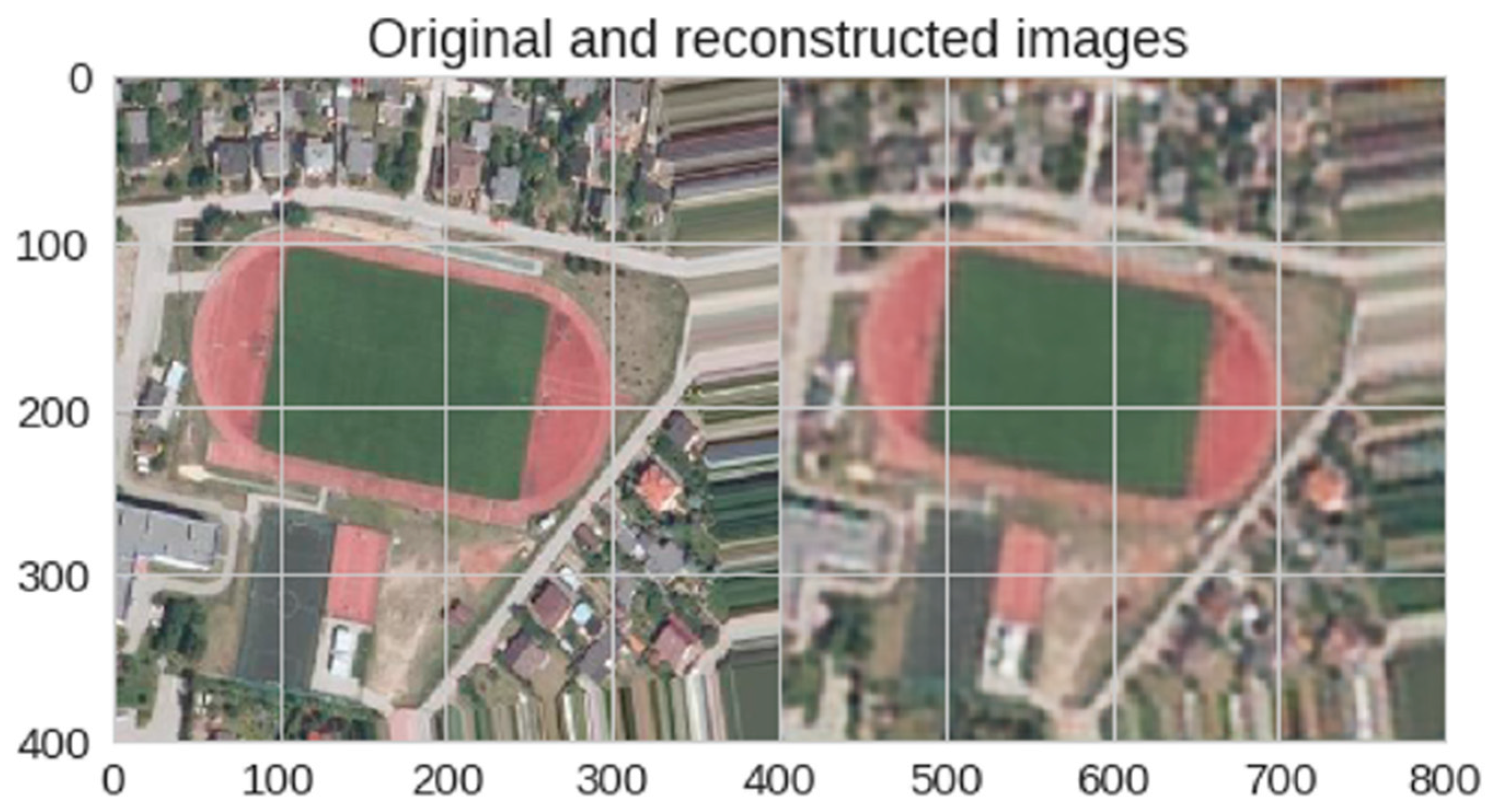
In general, autoencoders are defined from a process that encodes the input, a decoding process and a method that will calculate the loss between the input and the output image [31]. A very basic architecture of an encoder consists of one encoding and one decoding layer and, in this form, can be thought of as an advanced version of principal component analysis (PCA). The autoencoder trains itself in an unsupervised mode simply by presenting input data to the model, calculating the output (see Figure 1), and then using a backpropagation algorithm to minimize the cost function by adjusting the weights of the model. In that sense, autoencoders function as anomaly detectors. As autoencoders are trained to reconstruct the most resilient characteristics of a specific object, the cost to do so decreases. A trained model, when faced with an image of a different object, will manage to reconstruct it, but the error will be higher than expected. Thus, choosing a cost threshold enables an autoencoder to function as an anomaly detector. More advanced versions are deep learning autoencoders (DLAs), where each hidden layer is fully connected to the input of the next hidden layer.
Apart from anomaly detection [32,33], scene understanding for robotics [34], or 3D shape reconstruction [35], AEs have been used extensively in remote sensing [8,15,29,30] and have been proven to provide promising solutions to many classic remote sensing problems. For denoising and pan-sharpening images, a modified sparse denoising AE was used by [36] to learn the relationship between clean high-resolution images and low spatial/high spectral resolution images used as corrupted data. Similarly, Ref. [37] worked on the pan-sharpening problem by using a modified AE. For pixel-based classification, AE has been used with hyperspectral images (HSI) for feature extraction and image classification [38,39,40,41,42]. AE was used in [43] in order to extract both spatial and spectral features from HSI with a single network as part of a broader calcification process. For targeted feature recognition (e.g., ship, aircraft, or vehicle detection), AEs have been used to overcome challenges, such as a relatively small size and usually large number of targets and the complex neighboring environment [30,44].
2.4. Training Strategies
Another major decision is what kind of training strategy can be followed. In general, there are three different methods: (i) direct use of pre-trained networks, (ii) adapt pre-trained networks, and (iii) train a new network. While the first two options can have better overall results, they are out of scope of this research, given the restrictions set in the introduction. As [8] noted, the popular pre-trained networks are very large and contain millions of parameters to be learned. When used or re-trained with small training datasets, they will easily overfit (i.e., the model will memorize the parameters of the new small training set and will be unable to generalize in unseen images, thus it will perform poorly with unknown data). Reference [8] provides several examples in which researchers have opted to use smaller and completely new models and train them only with satellite images, so as to better handle remote sensing problems (see, for example, [30,45,46,47]). Interestingly, though, ref. [15] pointed out that in their review, most research efforts, and thus the pre-trained models suggested, focused on hyperspectral data or high spatial resolution images by using benchmark datasets, and therefore there is a limited number of studies that have focused on actual and practical applications of DL for remote sensing tasks.
2.5. ML/DL Challenges
Benchmark datasets are fundamental in several cases, as they provide a baseline to compare different options and methodologies. However, migrating from a benchmark dataset to the real world is not always a straightforward process, as there might be multiple challenges that have not been addressed in a lab-generated or hand-picked dataset. Reference [48] gives a detailed description of the problem and it is intriguing to follow the literature regarding how easy it is for deep neural networks (DNN), which are highly accurate on benchmark datasets, to be confused and perform poorly when they have to work with real-life adversarial cases. For example, [49] reported that with a set of adversarial images a DNN achieved an accuracy of approximately 2%, which was a drop of approximately 90% compared with its accuracy with the benchmark IMAGENET dataset. Similarly, [50] (p. 164) explored the “fundamental brittleness” (as François Chollet eloquently describes it) and presented multiple examples of how this can be achieved by using both artificial and natural adversarial images. For example, [51] showed how easy it is to create images that are impossible to recognize for humans but DNNs still assign them to a category with a confidence of 99.99%. Even small changes, such as translations, 2D rotations [52], or 3D rotations [53] of an image can completely fool a DNN. Moreover, it has been shown that small changes of texture or color cues can equally deteriorate the accuracy of DNN predictions [54]. In many of these cases, the image changes can be very subtle and not recognizable by a human, but still DNNs can give completely wrong predictions. Importantly, apart from changed images, unchanged natural images can also easily fool an otherwise accurate DNN [49]. So, as [55] summarized it, the evaluation of classifiers by their sheer performance on easy examples can make their deficiencies go unnoticed. This situation becomes even more confusing due to the fact that DNNs often report high confidence in their mistakenly inferred categories [49,51]. To date, it is not possible to provide a concrete solution to such problems, and thus fully trusting a DNN only by its confidence percentage might prove to be challenging and problematic, especially in emergency and life-critical processes [56].
Therefore, a possible option is to use ML/DL as an augmentation of human analysts and by doing so to move from a human-only process with multiple bottlenecks to a more automated process, yet preserving the quality of the results generated [2]. In this context, the methodology proposed is based on the fusion of human and artificial intelligence in order to develop a process that allows an expert to operate alongside DNNs.
3. Methodology
3.1. Data Acquisition
The first step was to locate inside the OSM database the crowd-contributed data for the soccer field category, which overlap the areas where satellite imagery is available. This was done with the help of the OSM Overpass Turbo Application Programming Interface (API). The requests returned as responses xml-based files, which were used by an algorithm in order to compute a 400 × 400 m rectangle around each soccer field. These rectangles were used later for cropping the satellite images. As the granularity of the OSM data can vary, soccer fields exist both as points and polygons inside the OSM database. In the cases where a soccer field was denoted as a single point, then this point was used as the center of the rectangle. If the soccer field was delineated with a polygon, then an envelope was computed around the soccer field feature, and the center of the envelope was used as the center for the computation of the 400 × 400 m rectangle.
The satellite images available for the research were acquired from many different sources from around Europe, and thus we can speculate that the images were captured with different sensors, and managed with different processes, transformations, and resampling methods, which were unknown to us and beyond our control. What was known is that the images were cloud-free, georeferenced (with unknown accuracy), three-channel (RGB), 8-bit pixel depth, JPEG compressed, and with a spatial resolution of 1 m.
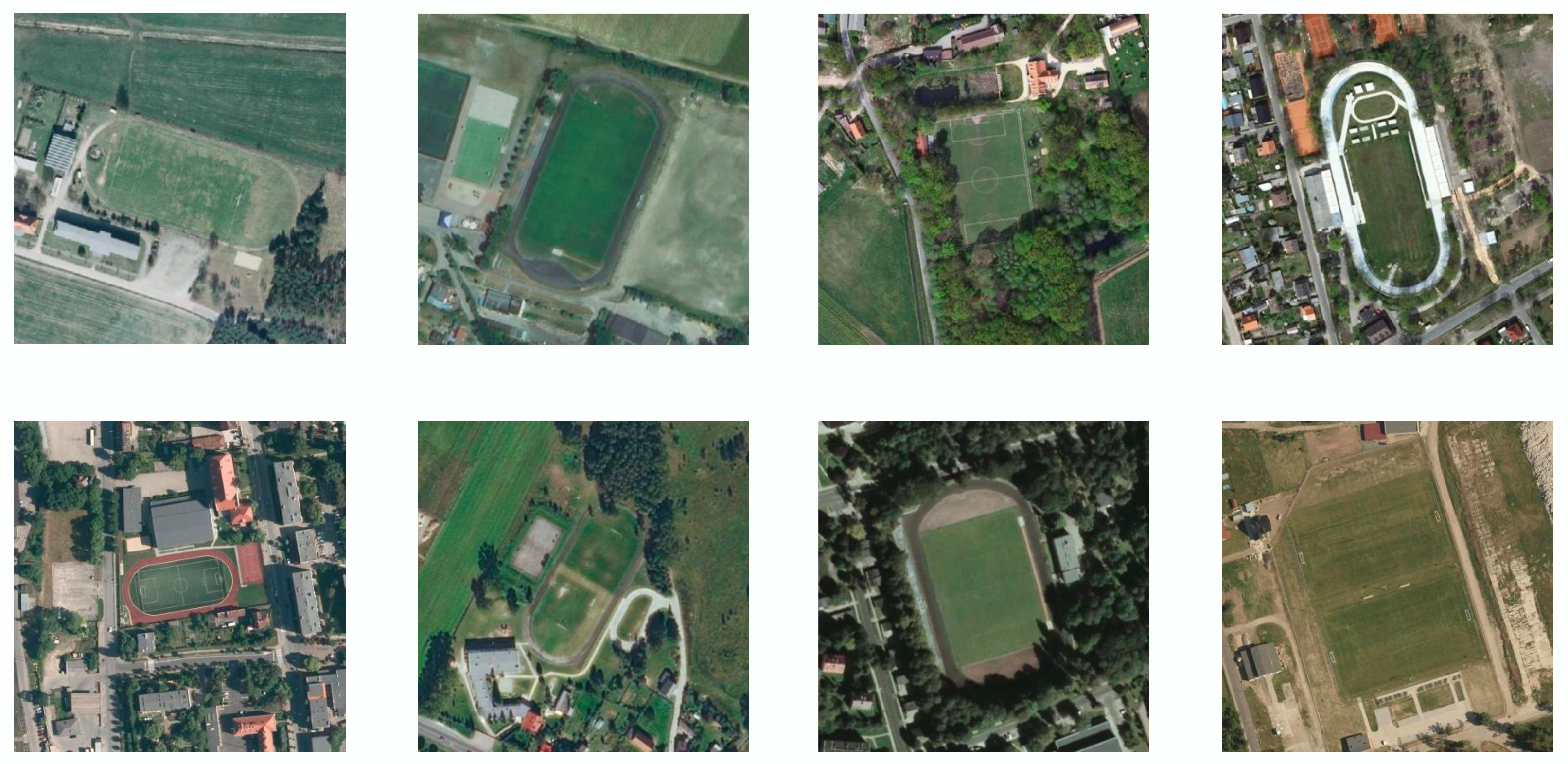
By using the 400 × 400 m rectangles described above, the images were automatically cropped, thus creating a dataset containing images of 400 × 400 pixels, samples of which can be seen in Figure 2. The soccer field features were of variable sizes and appeared in random rotation, thus a buffer zone needed to be decided. The choice of a 400 × 400 m rectangle (and thus cropping 400 × 400 pixel images) was arbitrary but it was based on an observation and a goal. The observation was that the OSM features did not always coincide with the features depicted in the images. This positional mismatch needed to be taken into account in order to have the entire feature inside the raw training image (although through the augmentation process this will not always be the case). The goal was to minimize the number of inferences that need to take place in order to examine an area. Therefore, the images should be large enough but still a considerable portion in each of them needs to be covered by the soccer field itself.
This process created a dataset of 2490 images and no further selection criteria were applied in order not to further reduce the image number, as this is already very small for training ML models, and in order to include possible natural adversarial images. A total of 250 random images were kept apart to be used in the evaluation process (see Section 3.3). For the remaining images, and in order to counterbalance the small training and validation samples, an augmentation process was followed by applying random dx, dy, and rotation factors. After the augmentation process the images were separated into two groups: the training group, with 9998 images, and the validating group, with 5243 images, with no overlaps. It could be argued that more training images could be acquired from the results provided by a search engine. However, as [49] explained, this would insert a bias in the training data, since search engines classify their images using CNNs. So, in practice, a search engine will return images that have been already classified as soccer fields by an ML/DL.
3.2. DLA and Training
The model used for training was a Deep Learning (or Stacked) Autoencoder (DLA). The architecture was decided through trial-and-error efforts, during which hyperparameter-tuning took place. During this fine-tuning process, each set of hyperparameters was evaluated through the monitoring of the training and validation loss. After a small number of epochs it was obvious if the parameters chosen were performing well or not. This considerably increased the speed of the methodology proposed. The aim was for the model to achieve a balance between minimum training time and best possible outcome, so that the whole process could serve the needs of an emergency response scenario.
The final architecture can be seen in Figure 3. The DLA consisted of three encoding layers, aiming to enable DLA to learn complex feature representations, and an equal number of symmetric decoding layers with the same padding. Each one of the encoding layers reduced the dimensionality of the input until a certain bottleneck, which held the most resilient characteristics of the input. The decoding layers inversed this procedure, aiming to reconstruct the initial input out of the latent space representation created during the encoding. After each deep layer, batch normalization was applied in order to adaptively normalize data, as the mean and variance change over time during the training process [57]. Also, in the encoding part, a max-pooling filter was applied for each deep layer, while an up-sampling filter was applied at the decoding part of the model. Both max-pooling and up-sampling used a 2 × 2 filter with steps equal to 1. Reference [58] explained that the down-sampling via pooling is needed to reduce the number of model parameters to process, as well as to induce spatial-filter hierarchies; at the same time, keeping the maximal activation (i.e., max-pooling) of the features over small patches has been proven to work better over other options (e.g., average-pooling). The activation of the layers was ReLU, while only the final decoder used sigmoid activation. ReLU (Rectified Linear Unit) is a function that moves negative values to zero: (f(x) = max(0,x)). Experience has showed that ReLU learns much faster and provides better results in networks with hidden layers, while sigmoid is a function (f(x) = 1/(1 + e^-x)) that moves arbitrary values into the [0, 1] interval [58,59,60]. The sigmoid output (i.e., from 0 up to 1) can be interpreted as a probability, and it was used only in the last output of the model. The optimizer used was adam (adaptive moment estimation), which computes individual adaptive learning rates for different parameters [61] and the loss function binary_crossentropy. The training of the model was made for 100 epochs using a batch size of 16. In total, the model had 11,083 parameters (10,971 trainable and 112 non-trainable).
For all the steps of the ML/DL process (i.e., data augmentation, model training, evaluation, and inference—see Section 4) the Google Colab (https://colab.research.google.com/) platform was used, which provides free access to both CPU and GPU processing power. In all steps the latter option was used since it is considerably faster. The training lasted for approximately three hours.
3.3. DLA Evaluation
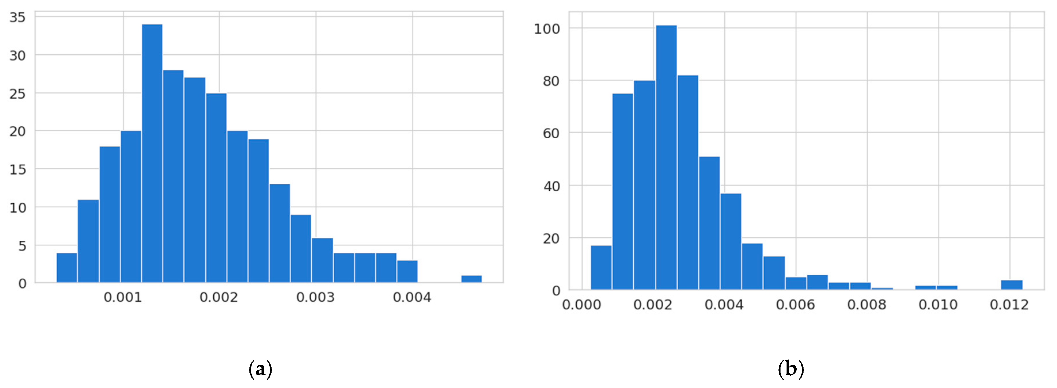
Every trained model was evaluated against a set of 250 positive and 500 negative (i.e., not including a soccer field) images in order to determine the reconstruction error threshold. For the selected model, the reconstruction errors for positive and negative images are shown in Figure 4.
Ideally, there should be no or very small overlap between the reconstruction error of positives and negatives. Since the DLA was trained in soccer field images only, the reconstruction error for those images (i.e., positives) should be small, while for other images (i.e., negatives) it should be bigger. If this was the case, then it would be easy to determine a threshold which clearly separated positives from negatives. However, as it can be seen, this was not the case. For example, although the reconstruction error frequencies (Figure 4) were different (see also Table 1), with the majority of positives having a reconstruction error less than 0.0025, while the majority of negatives had a bigger error than this, still, the overlap was considerably high. This would lead to many false negatives and false positives when the model would have to infer unseen images.
The small reconstruction errors in several negative images can be explained by the fact that some images are very easy to reconstruct (e.g., grass-land, water bodies). In order to tackle this challenge, an approach different to what is usually applied in deep learning applications was followed. The calculation of the DLA reconstruction error was made for each of the three image channels independently. Since DLA calculates the reconstruction error between the input and the output image, a separate error value was calculated for every channel. This was based on the assumption that in remote sensing, the relationships among the RGB channels are not meaningless, as in many image recognition problems. For example, the colors of a dog have no interrelation and probably play no or minimal role to the final categorization of an image as a dog or not. In contrast, in remote sensing, the pixel values of an RGB image have a meaningful role to play in object classification.
3.4. Infer Areas and Ground Truth Selection
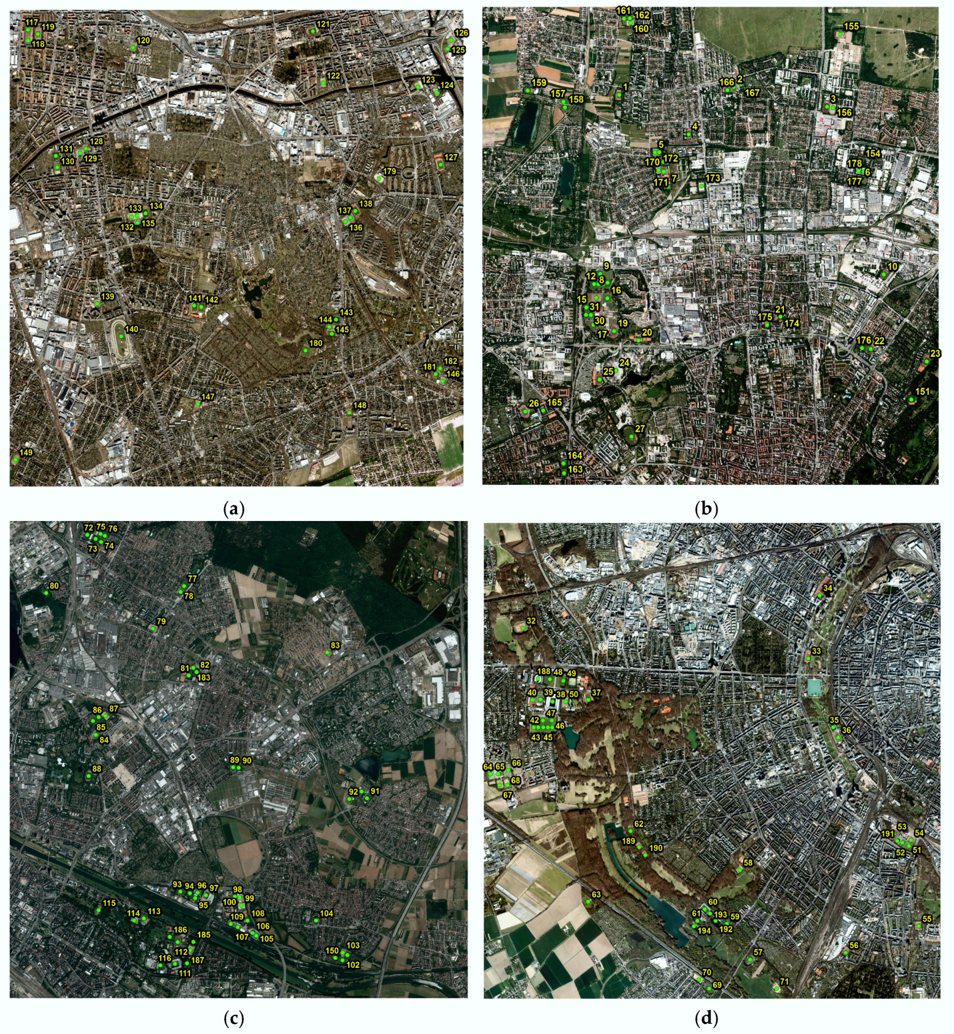
The inference evaluation of the model was made on satellite images, with similar origins and characteristics as the train images. These images covered four different areas in Germany: Berlin, Munich, Mannheim, and Cologne (Figure 5a–d). Each evaluation area was of equal size, 104.04 km2. The ground truth was manually verified and a total of 194 soccer fields were collected.
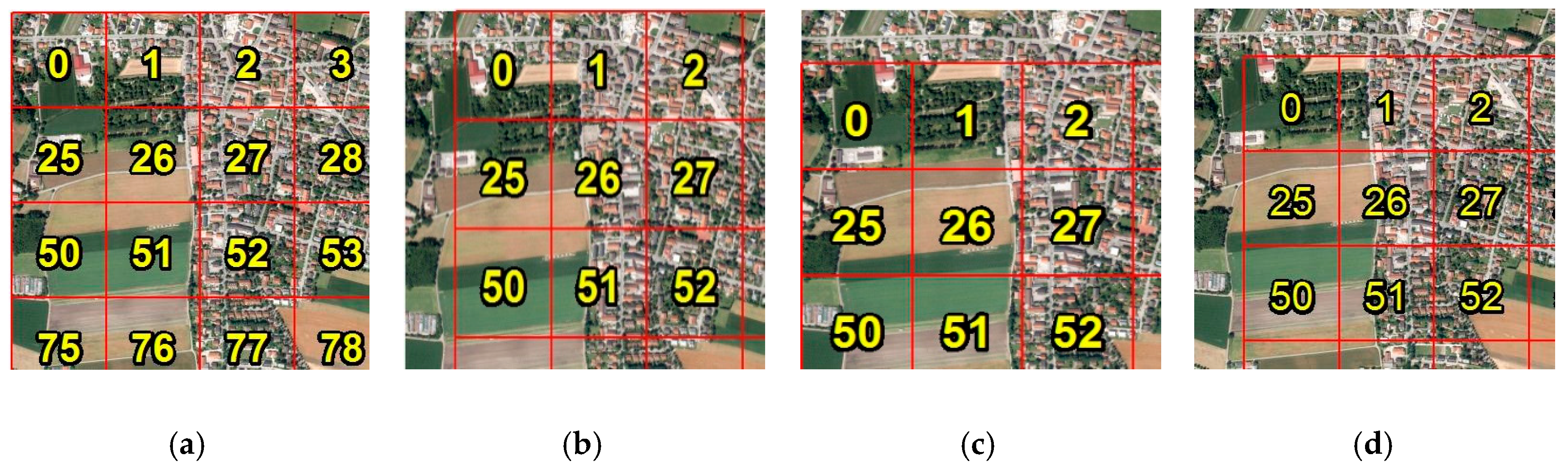
During the inference phase, each area was sliced in 625 tiles of 400 × 400 m. Each one of these tiles was inferred and a decision was made as to whether it contained a soccer field or not. In order to maximize the accuracy of the model, each area was examined four times (i.e., four passes), each time with a different slicing option, as seen in Figure 6, thus each time creating different tiles. This was decided in order to avoid tiles which contained part of a soccer field being classified as false negatives. This overhead does not affect the overall aim of a quick method as inference is a low-cost process in terms of time (e.g., each group of 625 tiles needs less than 2.5 min to be inferred).
Since during the training of the model, a reconstruction error was computed for every channel, a filter was set up to classify if an image qualified as positive or negative. The filter selected as positive any tile for which the reconstruction error was below the threshold for at least two channels. The tiles that had low reconstruction error and thus qualified for positives were grouped and their footprints were merged and dissolved. Thus, a polygon was created for each evaluation image which covered the area where possible positives existed (see also Figure 7—bright areas).
4. Results
For each evaluation area, Figure 7 shows the DLA-suggested possible positives areas (i.e., the areas that according to the model contain soccer fields) and the actual location of the soccer fields.
Given the initial goals set, the help that such an approach provides could be measured and evaluated with two different criteria. The first criterion was the reduction of the cognitive load of a user which otherwise has to manually pan through the entire area in order to locate all the possible soccer fields before continuing with further operational analysis. Table 2 shows the initial cognitive load, the cognitive load of the DLA, the actual reduction in km2, and the percentage of reduction. Then, Table 2 provides the area that the tiles of the ground truth cover and computes the initial and DLA overhead of cognitive load.
So, for example, for Berlin the model suggested a polygon of 26.04 km2 as possibly containing all the soccer fields of the specific area, thus reducing the initial cognitive load by 78 km2 or 75%. At the same time, the ground truth of the soccer fields covered 9.84 km2. Thus, compared to the initial area of 104 km2 the user would have a workload overhead of 957%, compared with the DLA area, for which the overhead was 165%. Overall, for all four cases, the cognitive load reduction was 70%, while the work overhead was reduced from 843% to 186%.
The second criterion was the accuracy of the model in terms of how many soccer fields were included in the suggested positive areas in relation to the overall number that existed in the selected areas. Table 3 shows the number of soccer fields identified in each area. Out of 194 soccer fields in total, in the areas suggested by the model, there were 166 soccer fields (i.e., 85.6%). The success rate ranged from 78% in Munich up to 91.5% in Cologne.
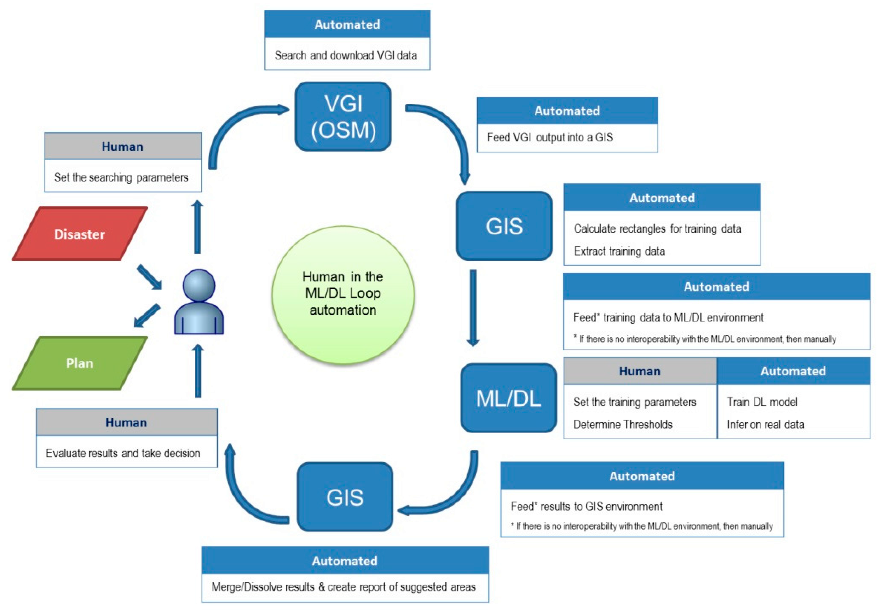
Overall, the methodology created a process (Figure 8) that can facilitate experts in dealing with increased and repetitive workload in resource-restricted environment. The methodology augments a core of ML/DL processes with well-known steps (such as the use of open source data or standard GIS tools) and requires minimal human intervention. While humans remain in the loop and have the final control in the decision-making process, the method eliminates bottlenecks and hastens reaction and planning.
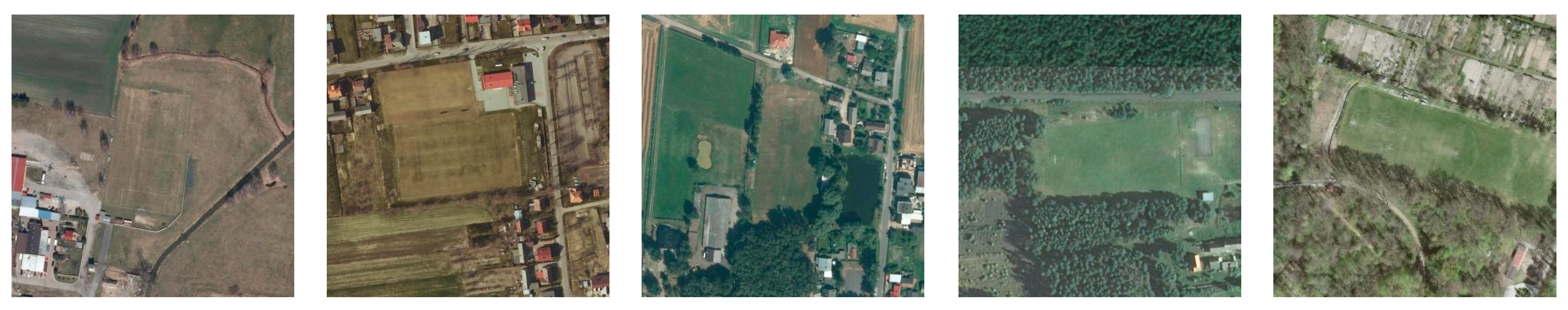
Finally, it is worth mentioning that in real life, the delineation of earth objects is not as clear as it usually appears in test data of other categories. For example, vehicle detection from high-resolution satellite images is facilitated by the fact that vehicles cannot easily blend with the background environment and their outlines are crisp and easier to detect. However, soccer fields, although they capture a much bigger area, are challenging to spot, as the borders with what is not soccer field can be extremely difficult to detect. Figure 9 shows a number of soccer field examples where the feature characteristics are not so obvious, and thus they are hard to classify correctly, even by an expert image analyst, especially when there is huge pressure in terms of time restrictions or work overload.
5. Discussion
The aim of this paper was to present an end-to-end methodology which could be used in a real-life disaster response scenario. The case examined was the location of soccer fields which, as explained in the introduction, qualify as very good areas for HLS. HLS analysis is a common task in relief supporting missions after a natural or man-made disaster. Moreover, HLS analysis has multiple applications in domains such as defense and security.
The process started by exploiting VGI data available in OSM. Through the available OSM API, the data could be downloaded and processed so as to be used in the creation of a pool of images that was split into training, validation, and evaluation datasets for a DL model to be trained. The datasets consisted of several RGB satellite images, automatically cropped around the soccer fields. In our case, the DL model selected was a DLA which was trained to function as an anomaly detector. The DLA was trained exclusively with soccer field images (raw and augmented) so as to be able to detect as an anomaly all other images that did not include a soccer field. Then, the trained model was used to infer four areas in order to suggest possible locations of soccer fields, while excluding the rest. In our case, the DLA managed to exclude 70% of the initial area and in the remaining 30% of the area, 85.6% of the actual soccer fields were identified.
The whole process is mostly automated as it needs minimal human intervention, while the transition from one step to the other is straightforward to program (in our case the Python programming language was used), whenever needed. Human input is needed to set the process in motion (i.e., to set the areas of interest at the OSM API or other open source data repository). The xml responses are parsed automatically and are fed into an algorithm that initially calculates the tile footprints and then performs the cropping of the images in order to create the training dataset. The training data need to be fed into the ML/DL algorithm. At the time of the research, the Google Colab project did not provide any API and thus this process was manual (i.e., to copy the data from the local GIS to Google Drive). However, this might change in the future. Moreover, newer versions of GIS have already incorporated AI functionality and thus the whole process could run under the same environment without interoperability issues. Another human intervention is needed for setting the training parameters and determining the threshold between positives and negatives. Then, the process can again become automated, as the inference process will only return the IDs of the candidate tiles. These are fed into an algorithm that selects the tile footprints, merges, and dissolves them.
The process takes a few hours to collect data, train a model, and use it with real-life imagery in order to get the final results. Given the restrictions discussed, we considered the results achieved in reducing the cognitive load and in successfully locating a high percentage of ground truth areas as very promising in such a degree that the process can be readily used in order to help the human agent in urgent and life-critical applications. The bottlenecks that can appear from the work overload or lack of image analysts in the first critical hours of a disaster response effort can be addressed with the help of ML/DL. The method presented does not aspire to create a fully automated disaster response mechanism but rather to keep the human in the loop of the decision process in order to ensure better understanding of the results and a meaningful decision on the best way to react.
There are several points through which the whole process can be improved in order to provide even better results. An obvious first step is to train the model for more time. The choice of 100 epochs was arbitrary and functioned more as a benchmark and less as a real training requirement. It is not uncommon for DLAs to be trained for thousands or tens of thousands of epochs. Another possible change could be the depth of the DLA—more convolution layers might allow the model to learn better and more useful data representations, thus enabling a more accurate anomaly detection. Similarly, the use of bigger training datasets can considerably improve the model’s performance. Often, DL models are trained in thousands or millions of images in order to attain high-accuracy results. However, all the above changes will severely affect the training time and thus a realistic balance must be sought, also taking into account that processing power will increase in the future.
Another group of changes could be implemented in the model architecture or in the use and adaptation of pre-trained layers, if there are enough new training data.
For example, an interesting approach would be to train from scratch models that are based on RNN or You Only Look Once (YOLO) [62] architecture. While these are considered part of future work, the discrepancies in granularity and geometric accuracy between VGI data and ground truth from satellite images have limited the usability of the crowdsourced labels, as in most cases, manual adjustment would be necessary. In particular, RNNs give a particular aspect in the problem, as they are designed to learn from sequential data. The case of soccer field detection could be considered as a special case of Land Use/Land Cover (LU/LC) classification, as it is not uncommon for rural soccer fields to be covered with regular grass that changes during the year, thus creating a sequence in their appearance. For LC classification RNNs have been used and [63] explained that the use of satellite image time series can be helpful to distinguish among classes, based on the fact they have different temporal profiles. Thus, the contribution of RNN in more complicated ML/DL models could be considered. However, RNNs are primarily strong when it comes to multitemporal datasets, as they can learn temporal dependencies [64]. They were first used for analyzing speech and time-series analysis and soon this ability was tested in remote sensing in order to characterize the sequential property of a hyperspectral pixel vector [65] or performing LULC with images from different dates [63,66], both of which were not easily applicable in our case. Regarding the use of pre-trained layers, [67] adjusted AlexNet (a more than 62M parameter CNN) for the classification of imagery-based Earth science phenomena, such as dust, hurricane, and smoke.
Another field of improvement can be the training data. As discussed, the training images were collected by different sensors and underwent different processes (e.g., resampling) and stored in different formats. Homogeneous data input can probably facilitate the model to better learn existing data representations. Moreover, the delineation of ground truth through the use of VGI data has not been so accurate, and thus, these mistakes have probably propagated into the DLA model [68]. Another possible change could be the size of the training images. Using smaller images (e.g., 300 × 300px) could enable a better model training, as the soccer field would be the dominant object inside each image and also allow time for longer training. The slight adjustment of other hyper-parameters, such as the convolution windows, strides, padding, or the batch size might result in a better model but, so far, the trial-and-error process followed before deciding on the specific values showed that any possible adjustments will not considerably improve the DLA performance, if the short training time is to be respected. Finally, as the ML process is part of a bigger hybrid human and AI process, the introduction of other spatial data in the process could considerably improve an HLS analysis. For example, combining the DLA outcome with other available data, such as river and lake polygons or road network, can further reduce the cognitive load of an image analyst. Even more intriguing is to introduce additional spatial data into the ML network itself, as in [69], who used LIDAR data in combination with RGB images or efforts that combined cross-views from aerial and ground geo-referenced images (from photo-sharing social networks) in order to detect objects (see, for example, [70,71]). However, such data are more difficult to acquire, especially after a disaster.
6. Conclusions
In a world where the flow of remotely-sensed data is constantly increasing, putting more man-power, shallow, or non-automated techniques into the analysis of imagery is proving to be insufficient for multiple applications. Time- and life-critical applications are particularly demanding and require novel approaches in order to avoid bottlenecks or errors. ML/DL methods provide solutions that can tackle both. However, it is understandable that there are multiple factors that can affect the outcome of an ML process in, so far, unknown and undocumented ways. AI might introduce potential sources of new biases that have not yet been studied, while at the same time the accuracy of the existing processes needs to be better understood and documented in order to be trusted. Therefore, despite the fact that research is evolving, hardware is getting more efficient and software (i.e., DL models) is becoming more and more accurate, the human factor still is and will continue to be a valuable asset in many decision-making processes, especially in life-critical cases. Nevertheless, we showed that it is feasible and applicable to develop processes that merge smoothly with existing practices, taking advantage of factors such as the existence of VGI or freely available GPU processing power, and can help the overall disaster response planning. Based on this, we support that methodologies that enable the intertwining of human and artificial intelligence are the way forward for critical decision making.
Author Contributions
Conceptualization, V.A. and C.P.; methodology, V.A.; software, V.A.; validation, V.A.; formal analysis, V.A.; investigation, resources, V.A.; data curation, V.A.; writing—original draft preparation, V.A.; writing—review and editing, V.A. and C.P.; visualization, V.A.; supervision, C.P. All authors have read and agreed to the published version of the manuscript.
Funding
This research received no external funding.
Acknowledgments
The authors would like to thank the two anonymous reviewers who helped to strengthen the manuscript with their insightful comments and guidance.
Conflicts of Interest
The authors declare no conflict of interest.
References
- Euroconsult. Euroconsult Research Projects Smallsat Market to Nearly Quadruple over Next Decade|Euroconsult. Available online: http://www.euroconsult-ec.com/5_August_2019 (accessed on 14 December 2019).
- Quinn, J.A.; Nyhan, M.M.; Navarro, C.; Coluccia, D.; Bromley, L.; Luengo-Oroz, M. Humanitarian applications of machine learning with remote-sensing data: review and case study in refugee settlement mapping. Philos. Trans. R. Soc. Math. Phys. Eng. Sci. 2018, 376, 20170363. [Google Scholar] [CrossRef] [PubMed] [Green Version]
- Santilli, G.; Vendittozzi, C.; Cappelletti, C.; Battistini, S.; Gessini, P. CubeSat constellations for disaster management in remote areas. Acta Astronaut. 2018, 145, 11–17. [Google Scholar] [CrossRef]
- United Nations; Australian Bureau of Statistics; Queensland University of Technology; Queensland Government; Commonwealth Scientific and Industrial Research Organisation; European Commission; National Institute of Statistics and Geography; Statistics Canada. Earth Observations for Official Statistics. 2019. Available online: https://unstats.un.org/bigdata/taskteams/satellite/UNGWG_Satellite_Task_Team_Report_WhiteCover.pdf (accessed on 11 February 2020).
- Yang, C.; Yu, M.; Li, Y.; Hu, F.; Jiang, Y.; Liu, Q.; Sha, D.; Xu, M.; Gu, J. Big Earth data analytics: A survey. Big Earth Data 2019, 3, 83–107. [Google Scholar] [CrossRef] [Green Version]
- Chi, M.; Plaza, A.; Benediktsson, J.A.; Sun, Z.; Shen, J.; Zhu, Y. Big Data for Remote Sensing: Challenges and Opportunities. Proc. IEEE 2016, 104, 2207–2219. [Google Scholar] [CrossRef]
- Ma, Y.; Wu, H.; Wang, L.; Huang, B.; Ranjan, R.; Zomaya, A.; Jief, W. Remote sensing big data computing: Challenges and opportunities. Future Gener. Comput. Syst. 2015, 51, 47–60. [Google Scholar] [CrossRef]
- Zhu, X.X.; Tuia, D.; Mou, L.; Xia, G.-S.; Zhang, L.; Xu, F.; Fraundorfer, F. Deep learning in remote sensing: A comprehensive review and list of resources. IEEE Geosci. Remote Sens. Mag. 2017, 5, 8–36. [Google Scholar] [CrossRef] [Green Version]
- Voigt, S.; Kemper, T.; Riedlinger, T.; Kiefl, R.; Scholte, K.; Mehl, H. Satellite Image Analysis for Disaster and Crisis-Management Support. IEEE Trans. Geosci. Remote Sens. 2007, 45, 1520–1528. [Google Scholar] [CrossRef]
- Kopp, S.; Becker, P.; Doshi, A.; Wright, D.J.; Zhang, K.; Xu, H. Achieving the Full Vision of Earth Observation Data Cubes. Data 2019, 4, 94. [Google Scholar] [CrossRef] [Green Version]
- Lewis, A.; Oliver, S.; Lymburner, L.; Evans, B.; Wyborn, L.; Mueller, N.; Gregory, R.; Hooke, J.; Woodcock, R.; Sixsmith, J.; et al. The Australian Geoscience Data Cube—Foundations and lessons learned. Remote Sens. Environ. 2017, 202, 276–292. [Google Scholar] [CrossRef]
- Giuliani, G.; Chatenoux, B.; Bono, A.D.; Rodila, D.; Richard, J.-P.; Allenbach, K.; Dao, H.; Peduzzi, P. Building an Earth Observations Data Cube: lessons learned from the Swiss Data Cube (SDC) on generating Analysis Ready Data (ARD). Big Earth Data 2017, 1, 100–117. [Google Scholar] [CrossRef] [Green Version]
- Gore, A. The digital earth: Understanding our planet in the 21st century. Photogramm. Eng. Remote Sens. 1999, 65, 528. [Google Scholar] [CrossRef]
- Craglia, M.; Bie, K.; de Jackson, D.; Pesaresi, M.; Remetey-Fülöpp, G.; Wang, C.; Annoni, A.; Bian, L.; Campbell, F.; Ehlers, M.; et al. Digital Earth 2020: Towards the vision for the next decade. Int. J. Digit. Earth 2012, 5, 4–21. [Google Scholar] [CrossRef]
- Ma, L.; Liu, Y.; Zhang, X.; Ye, Y.; Yin, G.; Johnson, B.A. Deep learning in remote sensing applications: A meta-analysis and review. ISPRS J. Photogramm. Remote Sens. 2019, 152, 166–177. [Google Scholar] [CrossRef]
- Yu, L.; Liang, L.; Wang, J.; Zhao, Y.; Cheng, Q.; Hu, L.; Liu, S.; Yu, L.; Wang, X.; Zhu, P.; et al. Meta-discoveries from a synthesis of satellite-based land-cover mapping research. Int. J. Remote Sens. 2014, 35, 4573–4588. [Google Scholar] [CrossRef]
- Maxwell, A.E.; Warner, T.A.; Fang, F. Implementation of machine-learning classification in remote sensing: an applied review. Int. J. Remote Sens. 2018, 39, 2784–2817. [Google Scholar] [CrossRef] [Green Version]
- He, K.; Sun, J. Convolutional Neural Networks at Constrained Time Cost. In Proceedings of the IEEE Conference on Computer Vision and Pattern Recognition, Boston, MA, USA, 7–12 June 2015; pp. 5353–5360. [Google Scholar]
- Harris, F.D.; Kasper, E.F.; Iseler, L.E. US Civil Rotorcraft Accidents, 1963 Through 1997; National Aeronautics and Space Administration Moffett Field: Fort Belvoir, VA, USA, 2000.
- Kovařík, V. Possibilities of geospatial data analysis using spatial modeling in ERDAS IMAGINE. In Proceedings of the International Conference on Military Technologies 2011-ICMT’11, At Brno, Czech Republic, 30–31 May 2011; pp. 1307–1313. [Google Scholar]
- Fitzgerald, D.; Walker, R.; Campbell, D. A Vision Based Forced Landing Site Selection System for an Autonomous UAV. In Proceedings of the 2005 International Conference on Intelligent Sensors, Sensor Networks and Information Processing, Melbourne, Australia, 5–8 December 2005; pp. 397–402. [Google Scholar]
- Scherer, S.; Chamberlain, L.; Singh, S. First results in autonomous landing and obstacle avoidance by a full-scale helicopter. In Proceedings of the IEEE International Conference on Robotics and Automation, Saint Paul, MN, USA, 14–18 May 2012; pp. 951–956. [Google Scholar]
- Maturana, D.; Scherer, S. 3D Convolutional Neural Networks for landing zone detection from LiDAR. In Proceedings of the IEEE International Conference on Robotics and Automation, Seattle, WA, USA, 26–30 May 2015. [Google Scholar]
- Haklay, M.; Antoniou, V.; Basiouka, S.; Soden, R.; Mooney, P. Crowdsourced Geographic Information Use in Government; World Bank Publications: Washington, DC, USA, 2014; pp. 1–73. [Google Scholar]
- Haklay, M.; Antoniou, V.; Basiouka, S.; Soden, R.J.; Deparday, V.; Sheely, R.M.; Mooney, P. Identifying Success Factors in Crowdsourced Geographic Information Use in Government; The World Bank: Washington, DC, USA, 2018; pp. 1–157. [Google Scholar]
- Ofli, F.; Meier, P.; Imran, M.; Castillo, C.; Tuia, D.; Rey, N.; Briant, J.; Millet, P.; Reinhard, F.; Parkan, M.; et al. Combining Human Computing and Machine Learning to Make Sense of Big (Aerial) Data for Disaster Response. Big Data 2016, 4, 47–59. [Google Scholar] [CrossRef] [Green Version]
- Chen, J.; Zhou, Y.; Zipf, A.; Fan, H. Deep Learning From Multiple Crowds: A Case Study of Humanitarian Mapping. IEEE Trans. Geosci. Remote Sens. 2018, 57, 1713–1722. [Google Scholar] [CrossRef]
- Krizhevsky, A.; Sutskever, I.; Hinton, G.E. ImageNet Classification with Deep Convolutional Neural Networks. In Advances in Neural Information Processing Systems 25; Pereira, F., Burges, C.J.C., Bottou, L., Weinberger, K.Q., Eds.; Curran Associates, Inc.: New York, NY, USA, 2012; pp. 1097–1105. [Google Scholar]
- Ball, J.E.; Anderson, D.T.; Chan, C.S. Feature and Deep Learning in Remote Sensing Applications. J. Appl. Remote Sens. 2017, 11, 42609. [Google Scholar]
- Zhang, L.; Zhang, L.; Du, B. Deep learning for remote sensing data: A technical tutorial on the state of the art. IEEE Geosci. Remote Sens. Mag. 2016, 4, 22–40. [Google Scholar] [CrossRef]
- Chollet, F. Building Autoencoders in Keras. Available online: https://blog.keras.io/building-autoencoders-in-keras.html (accessed on 14 December 2019).
- Chalapathy, R.; Menon, A.K.; Chawla, S. Anomaly Detection using One-Class Neural Networks. arXiv 2018, arXiv:1802.06360. [Google Scholar]
- Kwon, D.; Kim, H.; Kim, J.; Suh, S.C.; Kim, I.; Kim, K.J. A survey of deep learning-based network anomaly detection. Clust. Comput. 2019, 22, 949–961. [Google Scholar] [CrossRef]
- Cadena, C.; Dick, A.R.; Reid, I.D. Multi-modal Auto-Encoders as Joint Estimators for Robotics Scene Understanding. Robot. Sci. Syst. 2016, 12, 1–9. [Google Scholar]
- Feng, J.; Wang, Y. 3D shape retrieval using a single depth image from low-cost sensors. In Proceedings of the 2016 IEEE Winter Conference on Applications of Computer Vision (WACV), Lake Placid, NY, USA, 7–9 March 2016. [Google Scholar]
- Huang, W.; Xiao, L.; Wei, Z.; Liu, H. Songze Tang A New Pan-Sharpening Method with Deep Neural Networks. IEEE Geosci. Remote Sens. Lett. 2015, 12, 1037–1041. [Google Scholar] [CrossRef]
- Pan-sharpening via deep metric learning. ISPRS J. Photogramm. Remote Sens. 2018, 145, 165–183. [CrossRef]
- Lin, Z.; Chen, Y.; Zhao, X.; Wang, G. Spectral-spatial classification of hyperspectral image using autoencoders. In Proceedings of the 2013 9th International Conference on Information, Communications & Signal Processing, Kuala Lumpur, Malaysia, 10–13 December 2013. [Google Scholar]
- Chen, Y.; Lin, Z.; Zhao, X.; Wang, G.; Gu, Y. Deep Learning-Based Classification of Hyperspectral Data. IEEE J. Sel. Top. Appl. Earth Obs. Remote Sens. 2014, 7, 2094–2107. [Google Scholar] [CrossRef]
- Karalas, K.; Tsagkatakis, G.; Zervakis, M.; Tsakalides, P. Deep learning for multi-label land cover classification. In Image and Signal Processing for Remote Sensing XXI; International Society for Optics and Photonics: Toulouse, France, 2015; Volume 9643, p. 96430Q. [Google Scholar]
- Xing, C.; Ma, L.; Yang, X. Stacked Denoise Autoencoder Based Feature Extraction and Classification for Hyperspectral Images. J. Sens. 2016, 2016, 10. [Google Scholar] [CrossRef] [Green Version]
- Zabalzaa, J.; Rena, J.; Zhengb, J.; Zhaoc, H.; Qingd, C.; Yange, Z.; Duf, P.; Marshalla, S. Novel segmented stacked autoencoder for effective dimensionality reduction and feature extraction in hyperspectral imaging. Neurocomputing 2016, 185, 1–10. [Google Scholar] [CrossRef] [Green Version]
- Ma, X.; Wang, H.; Geng, J. Spectral–Spatial Classification of Hyperspectral Data Based on Deep Belief Network—IEEE Journals & Magazine. IEEE J. Sel. Top. Appl. Earth Obs. Remote Sens. 2016, 9, 4073–4085. [Google Scholar]
- Tang, J.; Deng, C.; Huang, G.-B.; Zhao, B. Compressed-Domain Ship Detection on Spaceborne Optical Image Using Deep Neural Network and Extreme Learning Machine. IEEE Trans. Geosci. Remote Sens. 2015, 53, 1174–1185. [Google Scholar] [CrossRef]
- Zou, Q.; Ni, L.; Zhang, T.; Wang, Q. Deep Learning Based Feature Selection for Remote Sensing Scene Classification. IEEE Geosci. Remote Sens. Lett. 2015, 12, 2321–2325. [Google Scholar] [CrossRef]
- Luus, F.P.S.; Salmon, B.P.; Bergh, F.; van den Maharaj, B.T.J. Multiview Deep Learning for Land-Use Classification. IEEE Geosci. Remote Sens. Lett. 2015, 12, 2448–2452. [Google Scholar] [CrossRef] [Green Version]
- Volpi, M.; Tuia, D. Dense Semantic Labeling of Subdecimeter Resolution Images with Convolutional Neural Networks. IEEE Trans. Geosci. Remote Sens. 2016, 55, 881–893. [Google Scholar] [CrossRef] [Green Version]
- Gilmer, J.; Adams, R.P.; Goodfellow, I.; Andersen, D.; Dahl, G.E. Motivating the Rules of the Game for Adversarial Example Research. arXiv 2018, arXiv:1807.06732. [Google Scholar]
- Hendrycks, D.; Zhao, K.; Basart, S.; Steinhardt, J.; Song, D. Natural Adversarial Examples. arXiv 2019, arXiv:1907.07174. [Google Scholar]
- Heaven, D. Why Deep-Learning AIs Are so Easy to Fool. Available online: https://www.nature.com/articles/d41586-019-03013-5 (accessed on 14 December 2019).
- Nguyen, A.; Yosinski, J.; Clune, J. Deep neural networks are easily fooled: High confidence predictions for unrecognizable images. In Proceedings of the IEEE Conference on Computer Vision and Pattern Recognition, Boston, MA, USA, 7–12 June 2015. [Google Scholar]
- Engstrom, L.; Tran, B.; Tsipras, D.; Schmidt, L.; Madry, A. Exploring the Landscape of Spatial Robustness. arXiv 2017, arXiv:1712.02779. [Google Scholar]
- Alcorn, M.A.; Li, Q.; Gong, Z.; Wang, C.; Mai, L.; Ku, W.-S.; Nguyen, A. Strike (with) a Pose: Neural Networks Are Easily Fooled by Strange Poses of Familiar Objects. In Proceedings of the IEEE Conference on Computer Vision and Pattern Recognition, Long Beach, CA, USA, 15–20 June 2019; pp. 4845–4854. [Google Scholar]
- Geirhos, R.; Rubisch, P.; Michaelis, C.; Bethge, M.; Wichmann, F.A.; Brendel, W. ImageNet-trained CNNs are biased towards texture; increasing shape bias improves accuracy and robustness. arXiv 2018, arXiv:1811.12231. [Google Scholar]
- Brendel, W.; Bethge, M. Approximating CNNs with Bag-of-local-Features models works surprisingly well on ImageNet. arXiv 2019, arXiv:1904.00760. [Google Scholar]
- Brown, T.B.; Carlini, N.; Zhang, C.; Olsson, C.; Christiano, P.; Goodfellow, I. Unrestricted Adversarial Examples. arXiv 2018, arXiv:1809.08352. [Google Scholar]
- Ioffe, S.; Szegedy, C. Batch Normalization: Accelerating Deep Network Training by Reducing Internal Covariate Shift. arXiv 2015, arXiv:1502.03167. [Google Scholar]
- Chollet, F. Deep Learning with Python; Manning Publications: Shelter Island, NY, USA, 2017; ISBN 978-1-61729-443-3. [Google Scholar]
- LeCun, Y.; Bengio, Y.; Hinton, G. Deep learning. Nature 2015, 521, 436–444. [Google Scholar] [CrossRef]
- Glorot, X.; Bordes, A.; Bengio, Y. Deep sparse rectifier neural networks. In Proceedings of the Fourteenth International Conference on Artificial Intelligence and Statistics, Ft. Lauderdale, FL, USA, 11–13 April 2011. [Google Scholar]
- Kingma, D.P.; Ba, J. Adam: A Method for Stochastic Optimization. arXiv 2017, arXiv:1412.6980. [Google Scholar]
- Redmon, J.; Divvala, S.; Girshick, R.; Farhadi, A. You Only Look Once: Unified, Real-Time Object Detection. arXiv 2016, arXiv:1506.02640. [Google Scholar]
- Ienco, D.; Gaetano, R.; Dupaquier, C.; Maurel, P. Land Cover Classification via Multi-temporal Spatial Data by Recurrent Neural Networks. IEEE Geosci. Remote Sens. Lett. 2017, 14, 1685–1689. [Google Scholar] [CrossRef] [Green Version]
- Ho Tong Minh, D.; Ienco, D.; Gaetano, R.; Lalande, N.; Ndikumana, E.; Osman, F.; Maurel, P. Deep Recurrent Neural Networks for Winter Vegetation Quality Mapping via Multitemporal SAR Sentinel-1. IEEE Geosci. Remote Sens. Lett. 2018, 15, 464–468. [Google Scholar] [CrossRef]
- Mou, L.; Ghamisi, P.; Zhu, X.X. Deep Recurrent Neural Networks for Hyperspectral Image Classification. IEEE Trans. Geosci. Remote Sens. 2017, 5, 3639–3655. [Google Scholar] [CrossRef] [Green Version]
- Lyu, H.; Lu, H.; Mou, L. Learning a Transferable Change Rule from a Recurrent Neural Network for Land Cover Change Detection. Remote Sens. 2016, 8, 506. [Google Scholar] [CrossRef] [Green Version]
- Maskey, M.; Ramachandran, R.; Miller, J. Deep learning for phenomena-based classification of Earth science images. J. Appl. Remote Sens. 2017, 11, 42608. [Google Scholar] [CrossRef]
- Xing, J.; Sieber, R.E. Propagation of Uncertainty for Volunteered Geographic Information in Machine Learning (Short Paper). In 10th International Conference on Geographic Information Science (GIScience 2018); Winter, S., Griffin, A., Sester, M., Eds.; Schloss Dagstuhl–Leibniz-Zentrum fuer Informatik: Dagstuhl, Germany, 2018; Volume 114, pp. 66:1–66:6. [Google Scholar]
- Campos-Taberner, M.; Romero-Soriano, A.; Gatta, C.; Camps-Valls, G.; Lagrange, A.; Saux, B.L.; Beaupère, A.; Boulch, A.; Chan-Hon-Tong, A.; Herbin, S.; et al. Processing of Extremely High-Resolution LiDAR and RGB Data: Outcome of the 2015 IEEE GRSS Data Fusion Contest–Part A: 2-D Contest. IEEE J. Sel. Top. Appl. Earth Obs. Remote Sens. 2016, 9, 5547–5559. [Google Scholar] [CrossRef] [Green Version]
- Lin, T.-Y.; Cui, Y.; Belongie, S.; Hays, J. Learning deep representations for ground-to-aerial geolocalization. In Proceedings of the IEEE Conference on Computer Vision and Pattern Recognition, Boston, MA, USA, 7–12 June 2015. [Google Scholar]
- Vo, N.N.; Hays, J. Localizing and Orienting Street Views Using Overhead Imagery. In Computer Vision—ECCV; Springer: Cham, Germany, 2016; pp. 494–509. [Google Scholar]
Figure 1.
The input and output of a deep learning autoencoder (DLA).

Figure 2.
Samples of the training dataset.

Figure 3.
The architecture of the DLA.

Figure 4.
Reconstruction error for the evaluation images: (a) positives, (b) negatives.

Figure 5.
Inference areas and ground truth for (a) Berlin; (b) Munich; (c) Mannheim; (d) Cologne.

Figure 6.
Different slicing methods (i.e., different dx, dy starting point) for the same area: (a) dx = dy = 0 m; (b) dx = 200 m, dy = 0 m; (c) dx = 0 m, dy = 200 m; (d) dx = dy = 200 m.
Figure 6.
Different slicing methods (i.e., different dx, dy starting point) for the same area: (a) dx = dy = 0 m; (b) dx = 200 m, dy = 0 m; (c) dx = 0 m, dy = 200 m; (d) dx = dy = 200 m.

Figure 7.
DLA-suggested areas where soccer fields existed and the actual ground truth (bright areas): (a) Berlin; (b) Munich; (c) Mannheim; (d) Cologne.
Figure 7.
DLA-suggested areas where soccer fields existed and the actual ground truth (bright areas): (a) Berlin; (b) Munich; (c) Mannheim; (d) Cologne.

Figure 8.
End-to-end ML/DL methodology for object identification.

Figure 9.
Different cases where it is difficult for soccer fields to be identified, even by expert image analysts.
Figure 9.
Different cases where it is difficult for soccer fields to be identified, even by expert image analysts.


Table 1.
Descriptive statistics of reconstruction errors for positives and negatives samples during the evaluation process.
Table 1.
Descriptive statistics of reconstruction errors for positives and negatives samples during the evaluation process.
| Descriptive Statistics | Positives | Negatives |
|---|---|---|
| count | 250 | 500 |
| mean | 0.001817 | 0.002829 |
| std | 0.000785 | 0.001737 |
| min | 0.000308 | 0.000242 |
| 25% | 0.001258 | 0.001711 |
| 50% | 0.001687 | 0.002507 |
| 75% | 0.002294 | 0.003468 |
| max | 0.004719 | 0.01236 |
Table 2.
DLA results on cognitive load (CL), ground truth, and work overhead compared to the initial task.
Table 2.
DLA results on cognitive load (CL), ground truth, and work overhead compared to the initial task.
| Inference Area | Initial CL (km2) | CL of DLA (km2) | Reduction of CL (km2) | % of CL Reduction | Ground Truth (km2) | % of Initial Overhead | % of DLA Overhead |
|---|---|---|---|---|---|---|---|
| Berlin | 104.04 | 26.04 | 78.00 | 74.7 | 9.84 | 957 | 165 |
| Munich | 104.04 | 20.25 | 83.79 | 80.5 | 12.45 | 736 | 63 |
| Mannheim | 104.04 | 47.56 | 56.48 | 54.3 | 11.08 | 839 | 329 |
| Cologne | 104.04 | 32.23 | 71.81 | 69.0 | 10.77 | 866 | 199 |
| Total | 416.16 | 126.08 | 290.08 | 70 | 44.14 | 166 | 85.6 |
| % of Total | - | 30.3 | - | - | 10.6 | - | - |
Table 3.
Soccer fields identified by the DLA.
| Inference Area | Ground Truth (Num. of Soccer Fields) | Num. of Soccer Fields Detected | % |
|---|---|---|---|
| Berlin | 37 | 32 | 86.5 |
| Munich | 59 | 46 | 78.0 |
| Mannheim | 51 | 45 | 88.2 |
| Cologne | 47 | 43 | 91.5 |
| Total | 194 | 166 | 85.6 |
© 2020 by the authors. Licensee MDPI, Basel, Switzerland. This article is an open access article distributed under the terms and conditions of the Creative Commons Attribution (CC BY) license (http://creativecommons.org/licenses/by/4.0/).
Share and Cite
MDPI and ACS Style
Antoniou, V.; Potsiou, C. A Deep Learning Method to Accelerate the Disaster Response Process. Remote Sens. 2020, 12, 544. https://doi.org/10.3390/rs12030544
AMA Style
Antoniou V, Potsiou C. A Deep Learning Method to Accelerate the Disaster Response Process. Remote Sensing. 2020; 12(3):544. https://doi.org/10.3390/rs12030544
Chicago/Turabian StyleAntoniou, Vyron, and Chryssy Potsiou. 2020. "A Deep Learning Method to Accelerate the Disaster Response Process" Remote Sensing 12, no. 3: 544. https://doi.org/10.3390/rs12030544
Note that from the first issue of 2016, this journal uses article numbers instead of page numbers. See further details here.