A Parallax Shift Effect Correction Based on Cloud Height for Geostationary Satellites and Radar Observations


Department of Geoinformatics, Faculty of Electronics, Telecommunications and Informatics, Gdańsk University of Technology, 11/12 Gabriela Narutowicza Street, 80-233 Gdańsk, Poland
Remote Sens. 2020, 12(3), 365; https://doi.org/10.3390/rs12030365
Submission received: 18 December 2019
/
Revised: 17 January 2020
/
Accepted: 19 January 2020
/
Published: 22 January 2020
(This article belongs to the Special Issue Radar and Sonar Imaging and Processing)
Abstract
:The effect of cloud parallax shift occurs in satellite imaging, particularly for high angles of satellite observations. This study demonstrates new methods of parallax effect correction for clouds observed by geostationary satellites. The analytical method that could be found in literature, namely the Vicente et al./Koenig method, is presented at the beginning. It approximates a cloud position using an ellipsoid with semi-axes increased by the cloud height. The error values of this method reach up to 50 meters. The second method, which is proposed by the author, is an augmented version of the Vicente et al./Koenig approach. With this augmentation, the error can be reduced to centimeters. The third method, also proposed by the author, incorporates geodetic coordinates. It is described as a set of equations that are solved with the numerical method, and its error can be driven to near zero by adjusting the count of iterations. A sample numerical solution procedure with application of the Newton method is presented. Also, a simulation experiment that evaluates the proposed methods is described in the paper. The results of an experiment are described and contrasted with current technology. Currently, operating geostationary Earth Observation (EO) satellite resolutions vary from 0.5 km up to 8 km. The pixel sizes of these satellites are much greater than for maximal error of the least precise method presented in this paper. Therefore, the chosen method will be important when the resolution of geostationary EO satellites reaches 50 m. To validate the parallax correction, procedure data from on-ground radars and the Meteosat Second Generation (MSG) satellite, which describes stormy events, was compared before and after correction. Comparison was performed by correlating the logarithm of the cloud optical thickness (COT) with radar reflectance in dBZ (radar reflectance – Z in logarithmic form).
Keywords:
parallax; cloud; earth observation; geostationary satellite; meteorological radar; MSG; SEVIRI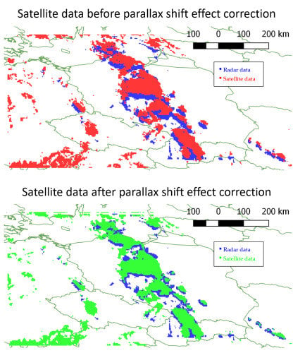
1. Introduction
The precision of remote space observations is important when investigating and monitoring various components of global ecological systems, such as marine, forestry, and climate environments [1,2,3,4]. Satellite data integration with external marine and other datasets is crucial in various applications of remote sensing techniques [5,6]. For climate and meteorological investigations, observations of clouds and precipitation on a global scale are usually performed using ground-based radar data and observations from geostationary satellites, due to their high temporal and moderate spatial resolution [7,8,9]. However, during data comparison and integration from these sources, the problem of parallax shift occurs [7,10], which is particularly observable for mid and high latitudes, and also for longitudes far from the sub-satellite point. Parallax shift is also important for cloud shadow determination, which is a significant issue for solar farms [11] and for flood detection [12]. Parallax phenomena also have a significant impact on the comparison of data from low-orbit satellites from different sensors [13,14,15,16].
In terms of mathematical problem formulation, the parallax shift effect for the geostationary satellites is actually a special case amongst low-orbit satellites, and it is easier to investigate due to higher temporal resolution data acquisition and the fixed satellite position.
There have been several attempts to solve parallax shift for geostationary satellites. One of them was proposed by Roebeling et al. [7,17,18], and was based on liquid water path (LWP) value pattern matching. This approach was suitable for stormy events and other inhomogeneous cloud formations, however it usually failed to perform correction in the case of homogeneous spatial LWP distribution. Another attempt proposed by Greuell et al. and Roebeling [19,20] used a simplified geometric model, which assumes Earth to be locally flat, as well as a sort of a priori knowledge about cloud height above the Earth’s surface. There were also attempts by Li, Sun, and Yu [12] to solve this problem using a spherical model. Finally, there is the Vicente et al./Koenig method [21,22] based on the geometric properties of parallax shift phenomena, incorporating an ellipsoid model of Earth. The Vicente et al./Koenig method will be presented further in this paper.
There are two methods proposed by the author in this paper, which are based on the same assumptions as the Vicente et al./Koenig method. The first is an augmented version of the mentioned method. This augmentation reduces the correction error to centimeters. The second method proposed by the author is an original work which is based as before on a priori knowledge of cloud height, a geodetic equation of an ellipsoid, and numerical methods for solving the equation set. This method allows the correction error to be reduced to almost zero (assuming Earth to have an ellipsoidal shape).
2. Nature of Parallax Shift Problem and Vicente et al./Koenig Method
2.1. Problem Description
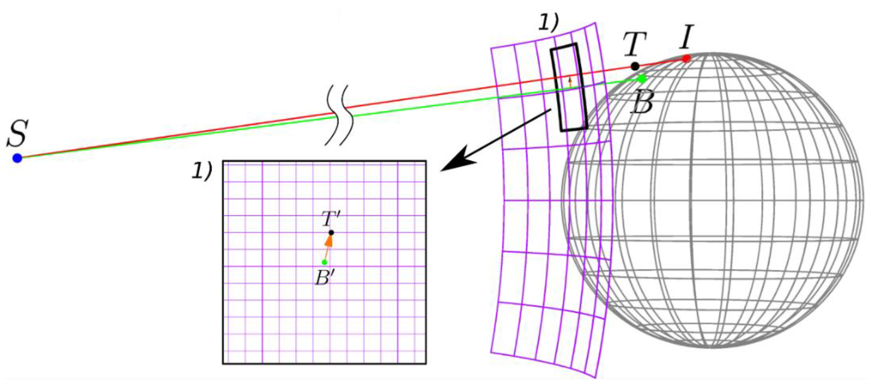
A parallax shift error in satellite observations occurs when the apparent image of the object is placed in the wrong location on the ellipsoid, considering the ellipsoid’s normal line passing through the observed point. This geometric phenomena is particularly observable in geostationary and polar satellite observations due to the high angles of observations, particularly for edge areas of image scenes. In Figure 1, the problem is presented considering the case of a geostationary satellite. As a result, this phenomena causes pixel drift from the original position towards the edge of the observation disk. Consequently, the higher the cloud top layer is, the bigger the shift that occurs.
The position of the cloud top (T) in Cartesian coordinates can be formulated as follows [23]:
where is the prime vertical radius of the curvature, is the square of eccentricity, is Earth’s semi-major axis, is Earth’s semi-minor axis, is the cloud top height, , is the geodetic latitude and longitude, and is the longitude above which the geostationary satellite is floating. In this case, Equation (1) models the cloud position on a tangent line at coordinates , (see Figure 2). This is a more precise model than the flat-earth model or the spherical model. Note that: all longitudes (, and ) are equal and the same. Subscripts are given to formally distinguish these values between corresponding latitudes that have different definitions (see Figure 2).
Pixel displacement in satellite view coordinates is defined as:
where and are constants that allow for sensor inclination angles to be converted to pixels or distance units in the satellite view space. Also, and are defined as:
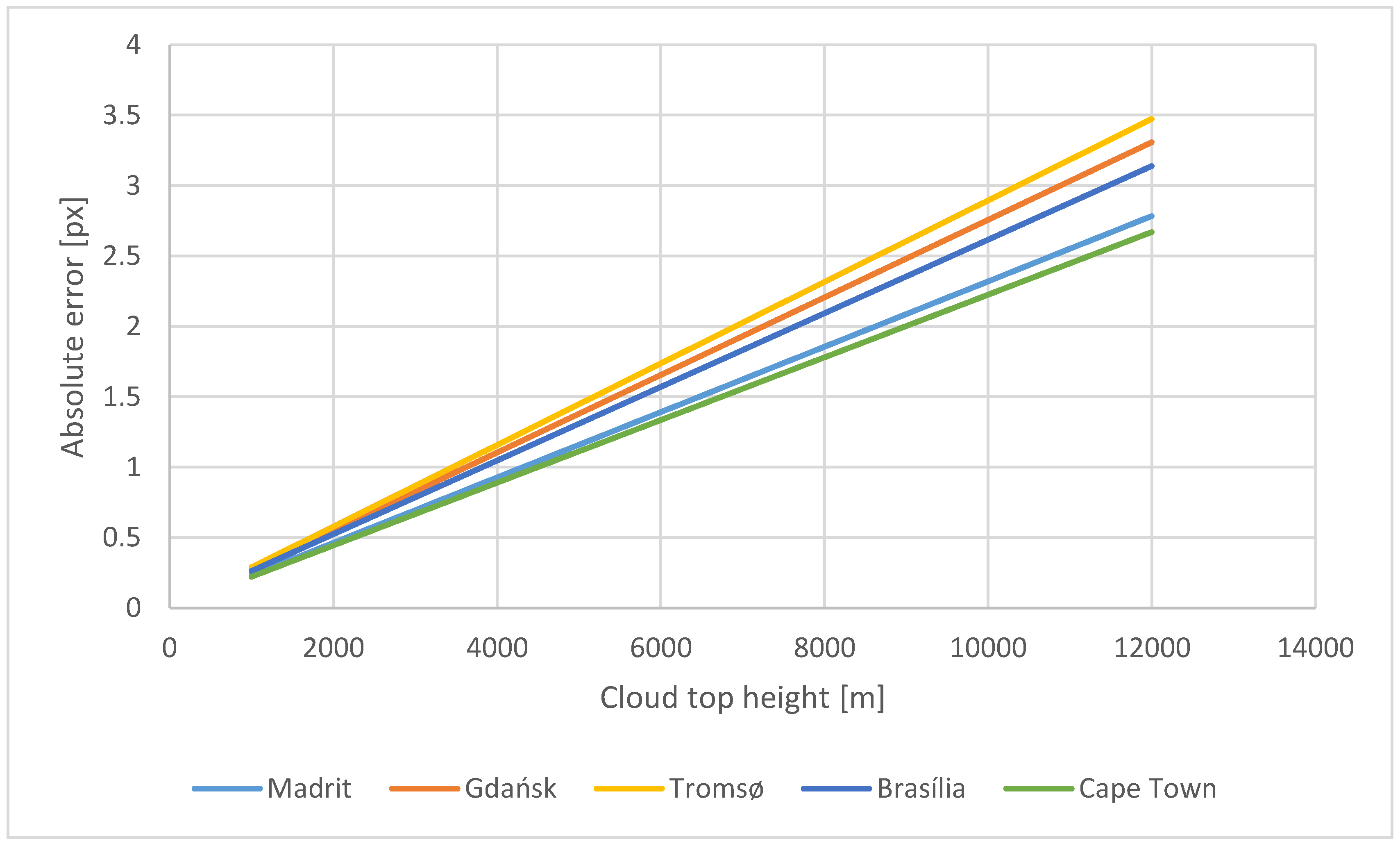
where , , and are cloud top coordinates from Equation (1) as functions of h; – distance from center of Earth to satellite; is the Earth’s semi-major axis; is the distance from the surface of Earth to the satellite. In order to illustrate , the following analysis presented in Figure 3 was performed. Namely, depending on the geographical localization of the affected pixel and cloud top height, the absolute shift error in observations is expressed in Spinning Enhanced Visible Infra-Red Imager (SEVIRI) pixel units (In this case ). It is worth noting that in many cases, especially for observations of clouds over 5000 m, this can cause pixel shift in the SEVIRI instruments used for the purpose of this study.
2.2. Vicente et al./Koenig Method
The parallax shift problem is solved using a geometrical model, assuming that the surface of Earth is an ellipsoid, and with a priori knowledge of cloud top height. One of the approaches considered in this work is the method proposed by Vicente et al. [21] and implemented by Marianne Koenig [22]. This approach, similar to the rest of the methods presented in this paper, assumes a priori knowledge of the cloud top height, which can be calculated using the observed brightness temperature [7,25]. In this method, the Cartesian coordinates of the cloud image are described as:
where is Earth’s semi-major axis; is Earth’s semi-minor axis; is the cloud top height; and are the geocentric latitude and longitude (see Figure 2), respectively; is the latitude of the geostationary satellite position; and is the local radius of ellipsoid for the geocentric latitude model:
where:
Satellite position (S) is defined as:
where is Earth’s semi-major axis and is the distance from the surface of Earth to the satellite.
The correction procedure is as follows:
- Designate satellite position in the Cartesian coordinates system;
- Designate the position of cloud top image in the Cartesian coordinates system using Equation (5);
- Designate vector ;
- Designate coefficient , which allows Cartesian coordinates of the cloud top to be calculated using the following equations (see Figure 5):where is described by the ellipsoid parametric equation:where and are the parametric latitude and longitude (see Figure 2). Therefore, Equation (9) can be presented as a set of equations:Squaring each equation and adding them according to their sides leads to a square equation, which can be solved with respect to c:
- Apply c to calculate the Cartesian coordinates of - , , and .
- Calculate the geocentric ellipsoidal coordinates of :
- If required for further computation, a geodetic latitude can be calculated:
Note that Equation (10) does not describe the cloud top position as it was defined in Equation (1) in Section 2.1. The coordinates of the point are shifted to height above the ellipsoid along the normal vector. Instead, it describes the point on the ellipsoid with the semi-axes increased by , therefore this method is burdened with error because of the inadequacy of the model.
3. Parallax Error Correction Methods with Lower Error
3.1. Vicente et al./Koenig Augmentation
The Vicente et al./Koenig method can be augmented in the final steps, where the latitude of the cloud bottom position is calculated. When using the Vicente et al./Koenig method, it is assumed that the cloud top is located on the ellipsoid with semi-axes increased by h, and therefore the geodetic latitude can be calculated taking into account the mentioned assumption:
If further computation requires the geocentric latitude, this can be calculated using the following equation:
This modification allows the correction error to be reduced to centimeters. Details will be presented in the experimental section.
3.2. Ellipsoid Model with Geodetic Coordinates: Numeric Method
This method incorporates the cloud top position defined in Section 2.1 in Equation (1). With the described cloud top position, the geostationary satellite observation line should be defined as:
where is the distance from Earth’s center to the satellite; is Earth’s semi-major axis; is the distance from the surface of Earth to the satellite; and are satellite inclination angles; is the distance from the satellite along the observation line. To solve this problem, an intersection point between the surface above the ellipsoid and the observation line needs to be calculated. Equations (1) and (17) should be merged, obtaining the following set of equations:
The root of the above system of equations ( and ) is the geodetic coordinates of point B. However, due to the entanglement of the variable in Equation (18), the root of the equations was designated using the numerical approach. The above method was implemented in C++ and Matlab. The Matlab implementation uses the fsolve function [26], which is part of the optimization toolbox. A detailed configuration of the fsolve function will be presented in the next section. The C++ implementation incorporates the Newton method, which is described below.
To solve the problem using the Newton method, the target function should be defined:
where:
In Equation (19), can be interpreted as the distance between the current solution and the optimal solution, which in the optimal case should be equal to zero. For such a defined cost function, calculation of the next iteration of the solution for the Newton method is defined as:
where:
and:
and:
The stopping condition is defined as:
However, the convergence of the above-presented approach is difficult to obtain for areas located near the edges of the observation disk. Therefore, an alternative target function is defined as the element-wise square of Equation (19):
with the gradient defined as:
and the stop condition:
Another issue that occurs in the numerical calculation problem is the big difference in scale between , which are expressed in radians, and , which is expressed in meters. To handle this problem, all distances () should be divided by . This operation will bring to a similar scale as .
4. Parallax Effect Correction Error Simulation
In order to compare the parallax effect correction obtained by the analyzed methods, a simulation experiment was performed. The main goal of the experiment was to generate several cloud top positions that simulate geostationary satellite observations, which result in and for simulated cloud top heights. With the and coordinates and a priori knowledge of the cloud height, correction methods were performed and their results were compared with the original (simulated) cloud position. The detailed procedure of the experiment is as follows:
- Prepare a grid of geodetic coordinates: , , with steps for each dimension;
- Transform the grid coordinates to the geostationary view coordinates system, , (from now on called the base , ) [27], and back to geodetic coordinates to specify which grid elements are out of scope; for out-of-scope elements, this operation will return Not a Number (NaN – floating point special value).
- For each , the following steps are performed:
- For each and and with , calculate the coordinates using Equation (1);
- Using , calculate the geostationary view coordinates and ;
- With , , and , run the correction algorithms: Vicente et al./Koenig, Vicente et al./Koenig augmented, and the numerical geodetic coordinates method;
- Each algorithm returns , , which should be transformed to , ;
- The distance between the simulated original base , and , in the geostationary view space will be denoted as the correction error.
The correction error is calculated in the geostationary view coordinate space (violet surface on Figure 1), because it allows the impact of the correction error on a specific satellite sensor to be estimated. The coordinates in the above equation were expressed as an angle, however expressing them in radians and multiplying by allows the result to be calculated in metric units (meters) as distances on a sphere of radius around a geostationary satellite. This interpretation of geostationary coordinates is implemented in the PROJ software library [28].
In order to calculate the correction using the geodetic coordinates numerical method, the fsolve [26] function was applied. All distances were normalized with respect to the radius of the equator. The parameters of the fsolve function were as follows:
- Algorithm: Levenberg–Marquardt (instead of Newton);
- Function tolerance: ;
- Specify objective gradient: yes;
- Input damping: .
The results of the simulation using the Vicente et al./Koenig method and its augmented version are presented in Figure 7 and Figure 8. The results using the geodetic coordinates numerical method are presented in Figure 9 and Figure 10.
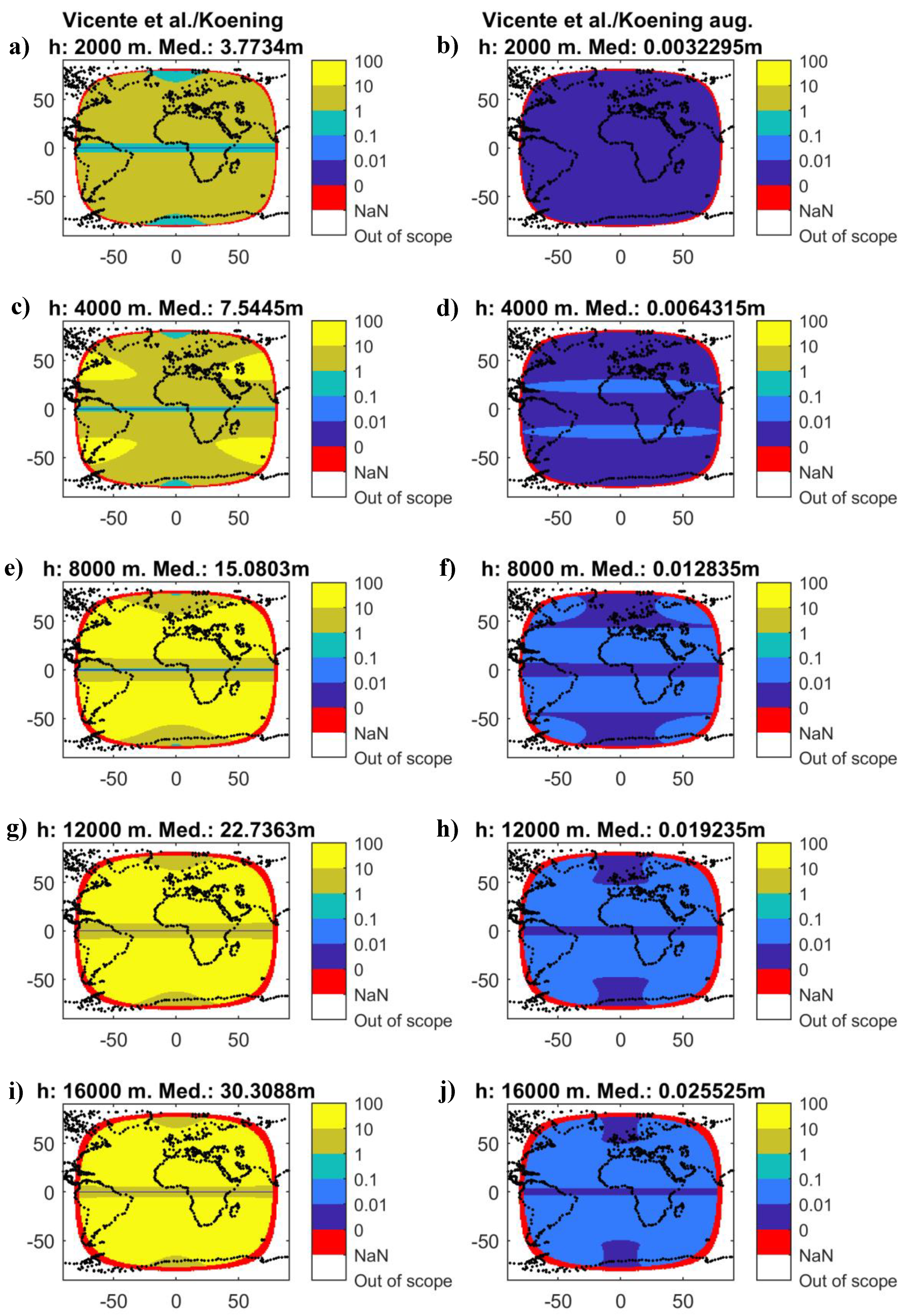
In Figure 7, the errors of the Vicente et al./Koenig method and its augmented version are depicted for certain cloud heights. Note that the error for the augmented version is times smaller than for the unmodified version. Also, the median of error rises near linearly with the increase of the cloud height. Also note that the error rises as the distance from the equator and from the central meridian increases.
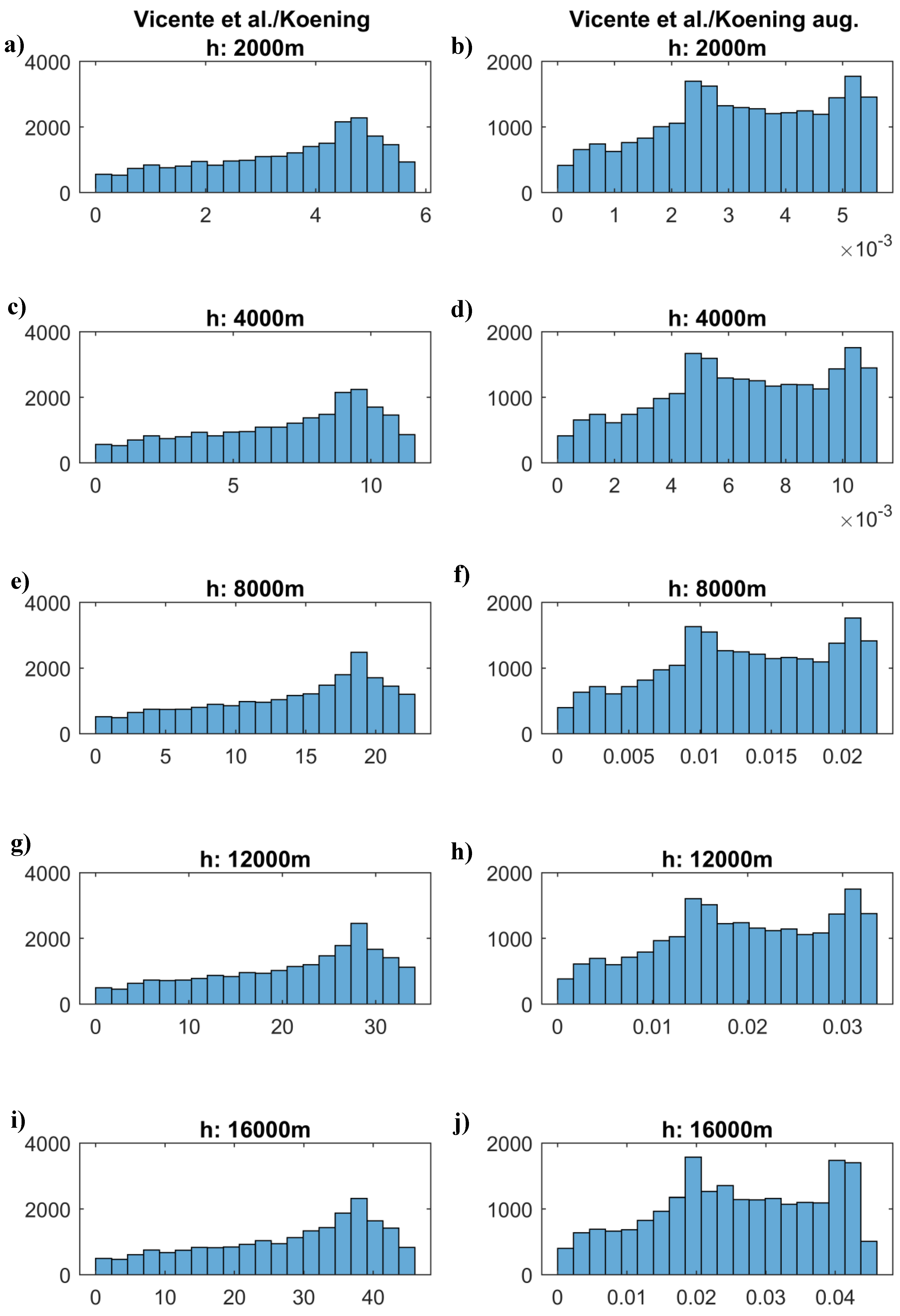
Figure 8 shows histograms of the errors presented in Figure 7. In the histograms, the error ratio between Vicente et al./Koenig and its augmented version can also be spotted, which can be estimated as . Another important piece of information is that for the assumed cloud heights, the maximal error of the Vicente et al./Koenig method can be estimated at 50 m, and for the augmented version, it can be estimated at 5 cm.
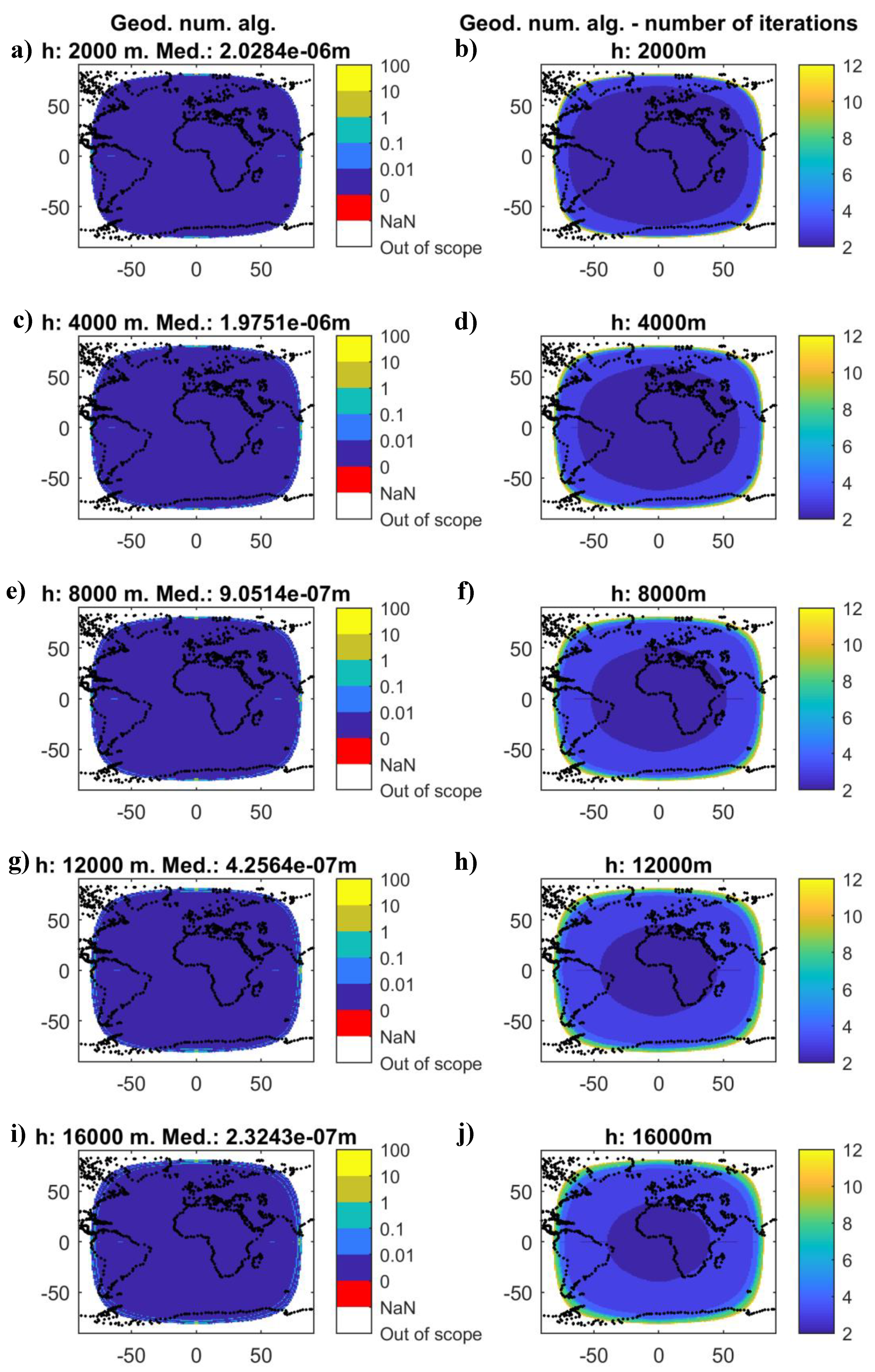
The errors of the geodetic coordinates numerical method for chosen cloud heights along with the number of iterations of the numerical method are shown in Figure 9. Note that the error is below 1 cm for almost the entire disc. The biggest errors appear near the edges in regions where the Vicente et al./Koenig method failed to compute a result (red NaN regions in Figure 7). The number of iterations increases as the height of the clouds and the distance from the center of the observation disc increase. However, during the performed experiments, the value for the majority of cases was less than or equal to five.
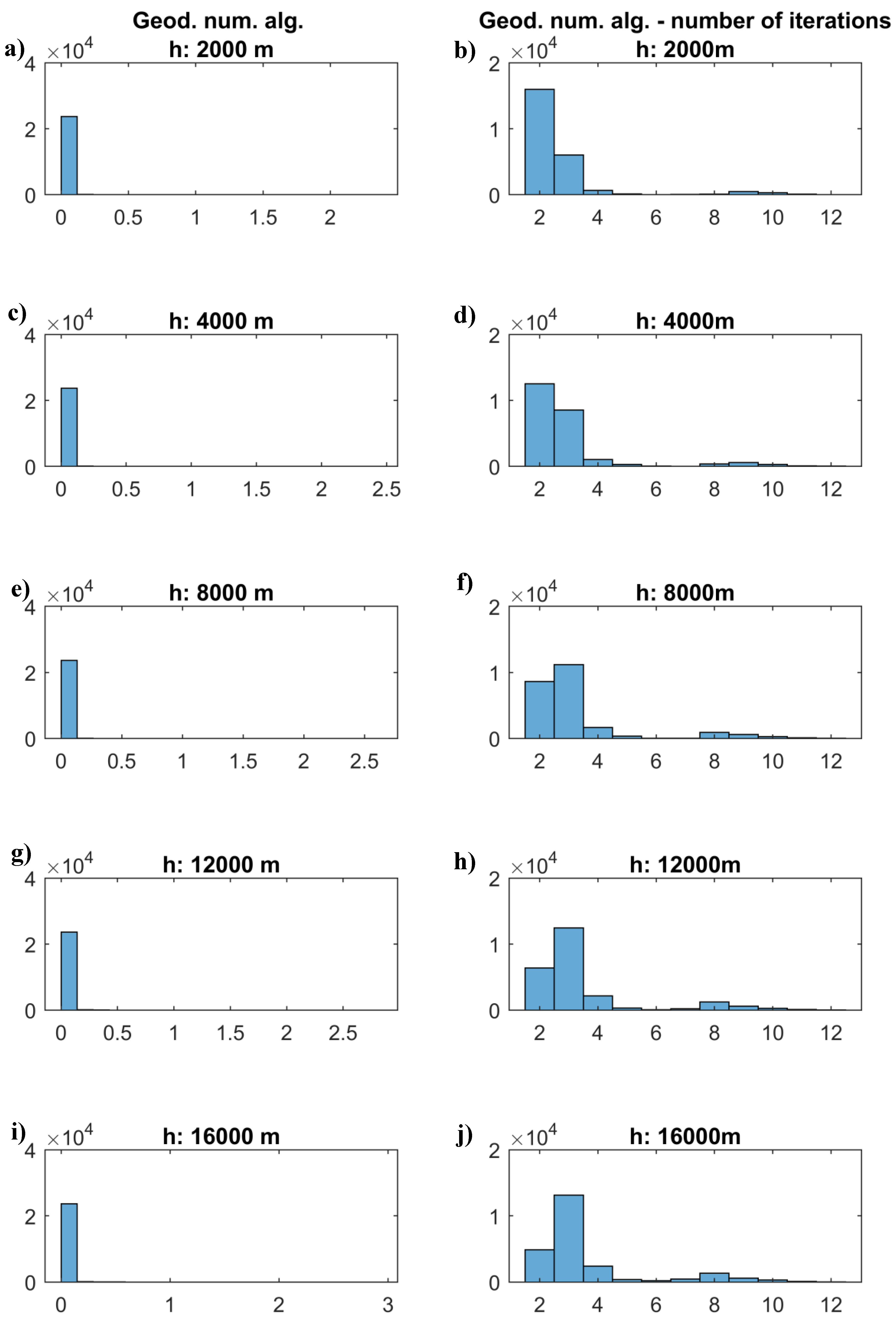
The histograms of errors for the geodetic coordinates numerical method and its number of iterations are presented in Figure 10. Based on the obtained results, the error histograms seem to be quite similar between the experiments—almost all values are classified as near zero. However, there are several occurrences of errors up to 3 meters, which are mainly caused by pixels in regions near the edge of the observation disc. The iteration histograms evolve along with the cloud height. As can be seen, the majority of occurrences fall below five iterations. Occurrences above this value refer to regions near the edge of the observation disc.
5. Discussion
The results of the conducted experiments indicate that the Vicente et al./Koenig parallax effect correction method error is smaller than 50 meters in the geostationary satellite coordinates system for cloud heights of up to 16 km. The error for the augmented version of the Vicente et al./Koenig method proposed by the author allows the error values to be decreased to below 10 cm, which is negligible for current practical applications. As expected, the error of the geodetic coordinates numerical method is also negligible because it can be adjusted by the number of iterations. However, the advantage of the numerical approach is that it corrects the positions of pixels located near the edge of the observation disc (there is no NaN on Figure 9).
On the other hand, it must be noted that the proposed approach requires greater computational power than a method with a constant number of steps, such as the Vicente et al./Koenig method. However, experiments show that this is negligible, as the parallax correction problem was computed within minutes.
As was mentioned in the introduction, parallax effect correction is significant for the comparison and collocation of meteorological radar data and geostationary satellite data. This can be demonstrated by comparing radar reflectance in dBZ:
where Z is radar reflectance. Reflectance is described as the following empirical relation with precipitation rate R [mm/h] [29]:
and cloud optical thickness (COT) in logarithmic form [30,31].
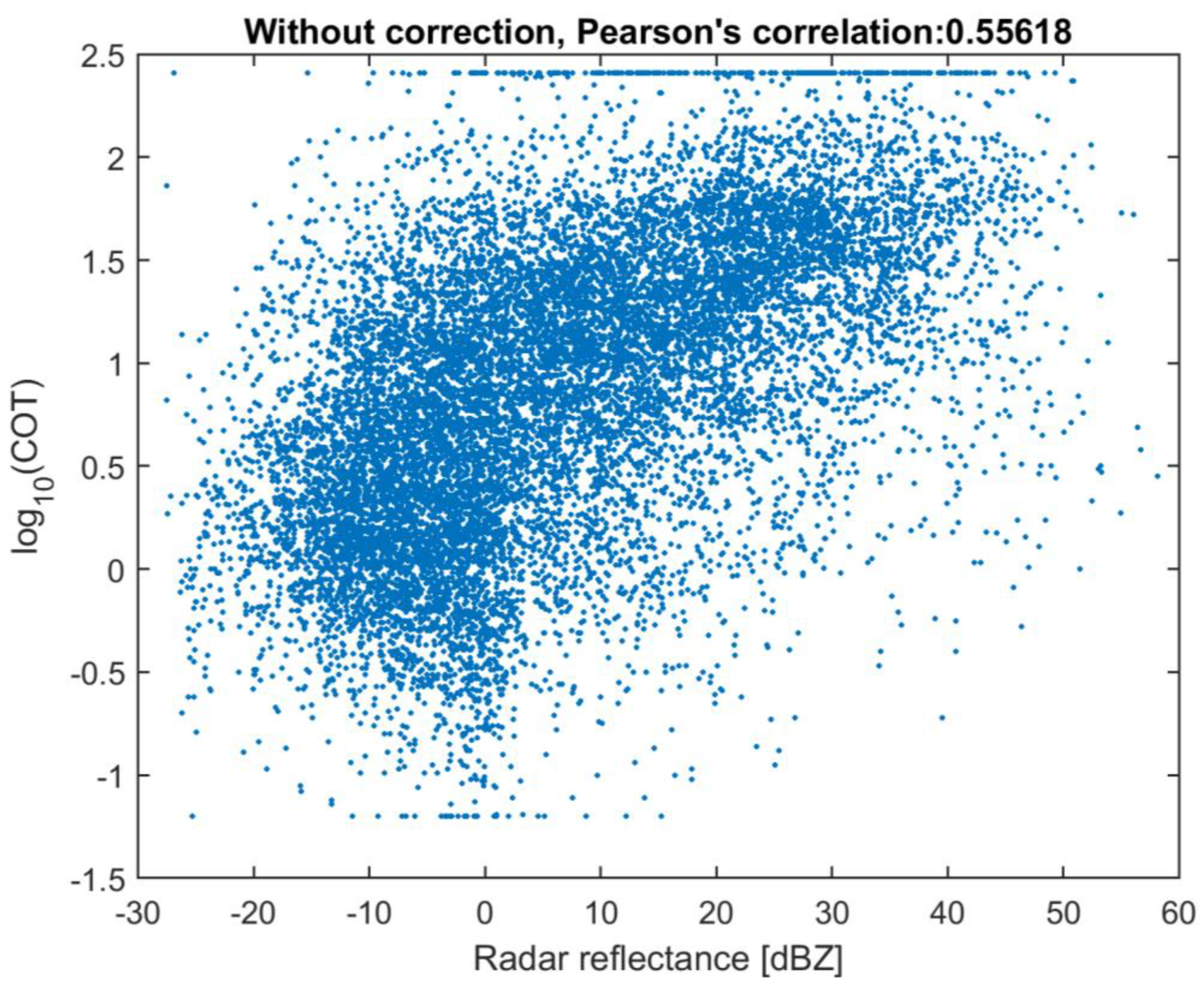
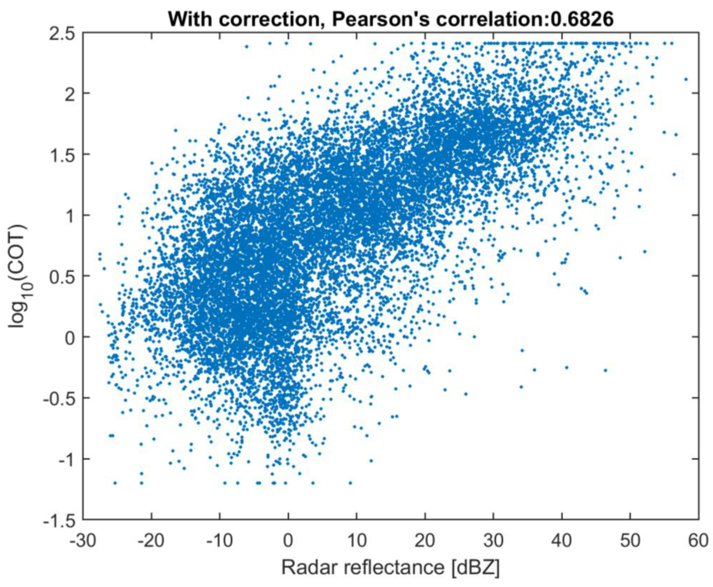
Figure 11 presents a scatterplot for radar reflectance and cloud optical thickness for satellite data without parallax effect correction, which should be mutually correlated in ideal cases. The Pearson’s correlation value for that case is equal to 0.556. On the other hand, Figure 12 presents the same type of scatterplot but for the satellite data after parallax effect correction (by numerical method from Section 3.2). The correlation value for the corrected data is equal to 0.683. Note that a threshold effect occurs on top of both figures (presented as a horizontal set of points equal to 2.4), which is a consequence of Optimal Cloud Analysis (OCA) algorithm look-up table (LUT) limitations [31]. It is worth noticing that this effect is less significant for Figure 12, suggesting that data with parallax effect corrections are improved in terms of geometric accuracy.
Note that despite performed spatial correction, data presented in Figure 6 and Figure 12 still differ. In this context, it is important to note that these differences are caused by other factors that influence data acquisition, namely:
- Different nature of the acquisition model, as on-ground radar and MSG satellite acquisition are registered with a slight temporal shift (less than 15 min);
- Both sensors utilize the different physical natures of acquisition. The on-ground radar is an active sensor which sends out an electromagnetic signal in the microwave spectrum and measurers the echo intensity scattered from precipitation particles. On the contrary, MSG SEVIRI is a passive sensor that measures radiation in a particular electromagnetic bandwidth (visible and near visible spectrum) coming from the sun and thermal radiance;
- Data acquired by MSG and on-ground radar is also characterized by different spatial resolutions. Therefore, in order to compare these datasets, additional resampling needs to be performed.
Another aspect worth considering is algorithm sensitivity to the uncertainty of cloud top height. The easiest way to approximate this is to calculate the sensitivity of the parallax error itself due to changes of cloud top height. The sensitivity of the parallax error in satellite coordinates is defined as a derivative of pixel displacement (Equation (2)) in respect to h:
Because pixel displacement is nearly linear in respect to h (as can be noticed on Figure 3), the derivative (Equation (31)) should nearly be constant for assumed and . Therefore, it can be approximated as the mean slope in respect to h, for instance:
where: . The displacement sensitivity depends on and , therefore its value varies around the globe. Sensitivity values for cities from Figure 3 are presented in Table 1.
Note that, the displacement sensitivity can be roughly approximated as less than 1. Therefore, SEVIRI instrument uncertainty of cloud height greater than or equal to 3 km may lead to one pixel size or greater error.
6. Conclusions
Data integration with data acquired from different sources requires developing additional methods that aim to reduce the discrepancies resulting from different physical aspects of observation. In this context, parallax shift correction for satellite data is a process that reduces geometric differences between observations, and in many cases can significantly improve the quality of corrected data in comparison with on-ground sources.
Regarding the scope of practical applications of the proposed approaches, it is important to note that the resolution of currently operating geostationary satellites varies between 1–3 km for a SEVIRI instrument [32] and 1–8 km for a Geostationary Operational Environmental Satellite (GOES) imager [33]. The upcoming series of Meteosat Third Generation (MTG) satellites will provide imagery with a spatial resolution between 0.5 and 2 km [34]. All of the above-presented parallax methods are effective enough for current and near future geostationary observation satellites, and the usefulness of the proposed methods is negligible. Selection of the proposed parallax effect correction method will be significant only when the spatial resolution of geostationary observations is comparable to 50 m. With high data resolution and precise parallax effect correction, the algorithm influence of precision on cloud height will become noticeable.
The parallax shift phenomena also affect the comparison between data collected from geostationary satellites and low-orbit satellites [14,35]. The parallax shift problem for geostationary satellites could be treated as a special case for low-orbit satellites. This problem for low-orbit satellites could be modeled with similar equations to those presented above, however taking into account the position and orientation of the satellite in the Cartesian coordinates space.
In this paper, the parallax effect was described using an ellipsoidal earth model. However, ellipsoidal model clearly does not fully reflect the real shape of Earth. Therefore, in situations where ellipsoidal model precision is insufficient, the numerical model of Earth’s gravitational field and geoid values should be utilized. In this case, it would be necessary to describe the parallax effects using differential equations and solve them using a numerical approach. In this case, the most problematic issue would be to determine perpendicular paths to the equipotential boundaries of Earth’s gravitational field.
Author Contributions
Conceptualization, T.B.; methodology, T.B.; software, T.B.; validation, T.B.; formal analysis, T.B.; investigation, T.B.; resources, T.B.; data curation, T.B.; writing—original draft preparation.; writing—review and editing, T.B.; visualization, T.B. All authors have read and agreed to the published version of the manuscript.
Funding
The research was supported under ministry subsidy for research for Gdansk University of Technology.
Acknowledgments
I would like to thank Andrzej Chybicki, PhD, and Tomasz Berezowski, PhD, for scientific and editorial support, as well as Marek Moszyński for supervising my work. Calculations were carried out thanks to the Academic Computer Centre in Gdańsk. Meteorological data from on-ground radars were provided by the Polish Institute of Meteorology and Water Management, National Research Institute.
Conflicts of Interest
The author declares no conflict of interest.
References
- Kaminski, L.; Kulawiak, M.; Cizmowski, W.; Chybicki, A.; Stepnowski, A.; Orlowski, A. Web-based GIS dedicated for marine environment surveillance and monitoring. In Proceedings of the OCEANS 2009-EUROPE, Bremen, Germany, 11–14 May 2009; pp. 1–7. [Google Scholar]
- Manzione, R.L.; Castrignano, A. A geostatistical approach for multi-source data fusion to predict water table depth. Sci. Total Environ. 2019, 696, UNSP 133763. [Google Scholar] [CrossRef] [PubMed]
- Mishra, M.; Dugesar, V.; Prudhviraju, K.N.; Patel, S.B.; Mohan, K. Precision mapping of boundaries of flood plain river basins using high-resolution satellite imagery: A case study of the Varuna river basin in Uttar Pradesh, India. J. Earth Syst. Sci. 2019, 128, 105. [Google Scholar] [CrossRef] [Green Version]
- Berezowski, T.; Wassen, M.; Szatylowicz, J.; Chormanski, J.; Ignar, S.; Batelaan, O.; Okruszko, T. Wetlands in flux: Looking for the drivers in a central European case. Wetl. Ecol. Manag. 2018, 26, 849–863. [Google Scholar] [CrossRef] [Green Version]
- Stateczny, A.; Bodus-Olkowska, I. Sensor data fusion techniques for environment modelling. In Proceedings of the 2015 16th International Radar Symposium (IRS), Bonn, Germany, 24–26 June 2015; pp. 1123–1128. [Google Scholar]
- Kazimierski, W.; Stateczny, A. Fusion of data from AIS and tracking radar for the needs of ECDIS. In Proceedings of the 2013 Signal Processing Symposium (SPS), Jachranka, Poland, 5–7 June 2013; pp. 1–6. [Google Scholar]
- Roebeling, R.A.; Holleman, I. SEVIRI rainfall retrieval and validation using weather radar observations. J. Geophys. Res. Atmos. 2009, 114. [Google Scholar] [CrossRef]
- Vicente, G.A.; Scofield, R.A.; Menzel, W.P. The Operational GOES Infrared Rainfall Estimation Technique. Bull. Amer. Meteor. Soc. 1998, 79, 1883–1898. [Google Scholar] [CrossRef]
- Zhao, J.; Chen, X.; Zhang, J.; Zhao, H.; Song, Y. Higher temporal evapotranspiration estimation with improved SEBS model from geostationary meteorological satellite data. Sci. Rep. 2019, 9, 14981. [Google Scholar] [CrossRef] [PubMed] [Green Version]
- Henken, C.C.; Schmeits, M.J.; Deneke, H.; Roebeling, R.A. Using MSG-SEVIRI Cloud Physical Properties and Weather Radar Observations for the Detection of Cb/TCu Clouds. J. Appl. Meteor. Climatol. 2011, 50, 1587–1600. [Google Scholar] [CrossRef]
- Miller, S.D.; Rogers, M.A.; Haynes, J.M.; Sengupta, M.; Heidinger, A.K. Short-term solar irradiance forecasting via satellite/model coupling. Solar Energy 2018, 168, 102–117. [Google Scholar] [CrossRef]
- Li, S.; Sun, D.; Yu, Y. Automatic cloud-shadow removal from flood/standing water maps using MSG/SEVIRI imagery. Int. J. Remote Sens. 2013, 34, 5487–5502. [Google Scholar] [CrossRef]
- Wang, C.; Luo, Z.J.; Huang, X. Parallax correction in collocating CloudSat and Moderate Resolution Imaging Spectroradiometer (MODIS) observations: Method and application to convection study. J. Geophys. Res. Atmos. 2011, 116. [Google Scholar] [CrossRef] [Green Version]
- Guo, Q.; Feng, X.; Yang, C.; Chen, B. Improved Spatial Collocation and Parallax Correction Approaches for Calibration Accuracy Validation of Thermal Emissive Band on Geostationary Platform. IEEE Trans. Geosci. Remote Sens. 2018, 56, 2647–2663. [Google Scholar] [CrossRef]
- Chen, J.; Yang, J.-G.; An, W.; Chen, Z.-J. An Attitude Jitter Correction Method for Multispectral Parallax Imagery Based on Compressive Sensing. IEEE Geosci. Remote Sens. Lett. 2017, 14, 1903–1907. [Google Scholar] [CrossRef]
- Frantz, D.; Haß, E.; Uhl, A.; Stoffels, J.; Hill, J. Improvement of the Fmask algorithm for Sentinel-2 images: Separating clouds from bright surfaces based on parallax effects. Remote Sens. Environ. 2018, 215, 471–481. [Google Scholar] [CrossRef]
- Roebeling, R.A.; Feijt, A.J. Validation of cloud liquid water path retrievals from SEVIRI on METEOSAT-8 using CLOUDNET observations. In Proceedings of the EUMETSAT Meteorological Satellite Conference, Helsinki, Finland, 12–16 June 2006; EUMETSAT: Darmstadt, Germany, 2006; pp. 12–16. [Google Scholar]
- Roebeling, R.A.; Deneke, H.M.; Feijt, A.J. Validation of Cloud Liquid Water Path Retrievals from SEVIRI Using One Year of CloudNET Observations. J. Appl. Meteor. Climatol. 2008, 47, 206–222. [Google Scholar] [CrossRef]
- Greuell, W.; Roebeling, R.A. Toward a Standard Procedure for Validation of Satellite-Derived Cloud Liquid Water Path: A Study with SEVIRI Data. J. Appl. Meteor. Climatol. 2009, 48, 1575–1590. [Google Scholar] [CrossRef] [Green Version]
- Schutgens, N.A.J.; Greuell, W.; Roebeling, R. Effect of inhomogeneity on the validation of SEVIRI LWP. In Current Problems in Atmospheric Radiation (irs 2008); Nakajima, T., Yamasoe, M.A., Eds.; Amer Inst Physics: New York, NY, USA, 2009; Volume 1100, p. 424. ISBN 978-0-7354-0635-3. [Google Scholar]
- Vicente, G.A.; Davenport, J.C.; Scofield, R.A. The role of orographic and parallax corrections on real time high resolution satellite rainfall rate distribution. Int. J. Remote Sens. 2002, 23, 221–230. [Google Scholar] [CrossRef]
- Koenig, M. Description of the parallax correction functionality. Available online: https://cwg.eumetsat.int/parallax-corrections/ (accessed on 17 January 2020).
- Wolfgang, T. Geodesy, An Introduction; De Gruyter: Berlin, Germany, 1980; ISBN 3-11-007232-7. [Google Scholar]
- Czarnecki, K. Geodezja współczesna; Wyd. 3 (1 w WN PWN)-1 dodruk; Wydawnictwo Naukowe PWN: Warszawa, Poland, 2015; ISBN 978-83-01-18380-6. [Google Scholar]
- Meteorological Products Extraction Facility Algorithm Specification Document. Available online: https://www.eumetsat.int/website/wcm/idc/idcplg?IdcService=GET_FILE&dDocName=PDF_TEN_SPE_04022_MSG_MPEF&RevisionSelectionMethod=LatestReleased&Rendition=Web (accessed on 28 November 2019).
- Solve System of Nonlinear Equations - MATLAB Fsolve. Available online: https://www.mathworks.com/help/optim/ug/fsolve.html (accessed on 23 October 2019).
- Wolf, R. Coordination Group for Meteorological Satellites LRIT/HRIT Global Specification. Available online: https://www.cgms-info.org/documents/pdf_cgms_03.pdf (accessed on 28 November 2019).
- PROJ contributors. PROJ Coordinate Transformation Software Library; Open Source Geospatial Foundation: Beaverton, OR, USA, 2019. [Google Scholar]
- Marshall, J.S.; Gunn, K.L.S. Measurement of snow parameters by radar. J. Meteor. 1952, 9, 322–327. [Google Scholar] [CrossRef] [Green Version]
- Roebeling, R.A.; Feijt, A.J.; Stammes, P. Cloud property retrievals for climate monitoring: Implications of differences between Spinning Enhanced Visible and Infrared Imager (SEVIRI) on METEOSAT-8 and Advanced Very High Resolution Radiometer (AVHRR) on NOAA-17. J. Geophys. Res. Atmos. 2006, 111. [Google Scholar] [CrossRef]
- Optimal Cloud Analysis: Product Guide. Available online: http://www.eumetsat.int/website/wcm/idc/idcplg?IdcService=GET_FILE&dDocName=PDF_DMT_770106&RevisionSelectionMethod=LatestReleased&Rendition=Web (accessed on 8 January 2020).
- MSG Level 1. Available online: http://www.eumetsat.int/website/wcm/idc/idcplg?IdcService=GET_FILE&dDocName=PDF_TEN_05105_MSG_IMG_DATA&RevisionSelectionMethod=LatestReleased&Rendition=Web (accessed on 28 November 2019).
- GOES N Databook. Available online: https://goes.gsfc.nasa.gov/text/GOES-N_Databook/databook.pdf (accessed on 29 November 2019).
- MTG FCI L1 Product User Guide. Available online: http://www.eumetsat.int/website/wcm/idc/idcplg?IdcService=GET_FILE&dDocName=PDF_DMT_719113&RevisionSelectionMethod=LatestReleased&Rendition=Web (accessed on 28 November 2019).
- Hewison, T.J. An Evaluation of the Uncertainty of the GSICS SEVIRI-IASI Intercalibration Products. IEEE Trans. Geosci. Remote Sens. 2013, 51, 1171–1181. [Google Scholar] [CrossRef]
Figure 1.
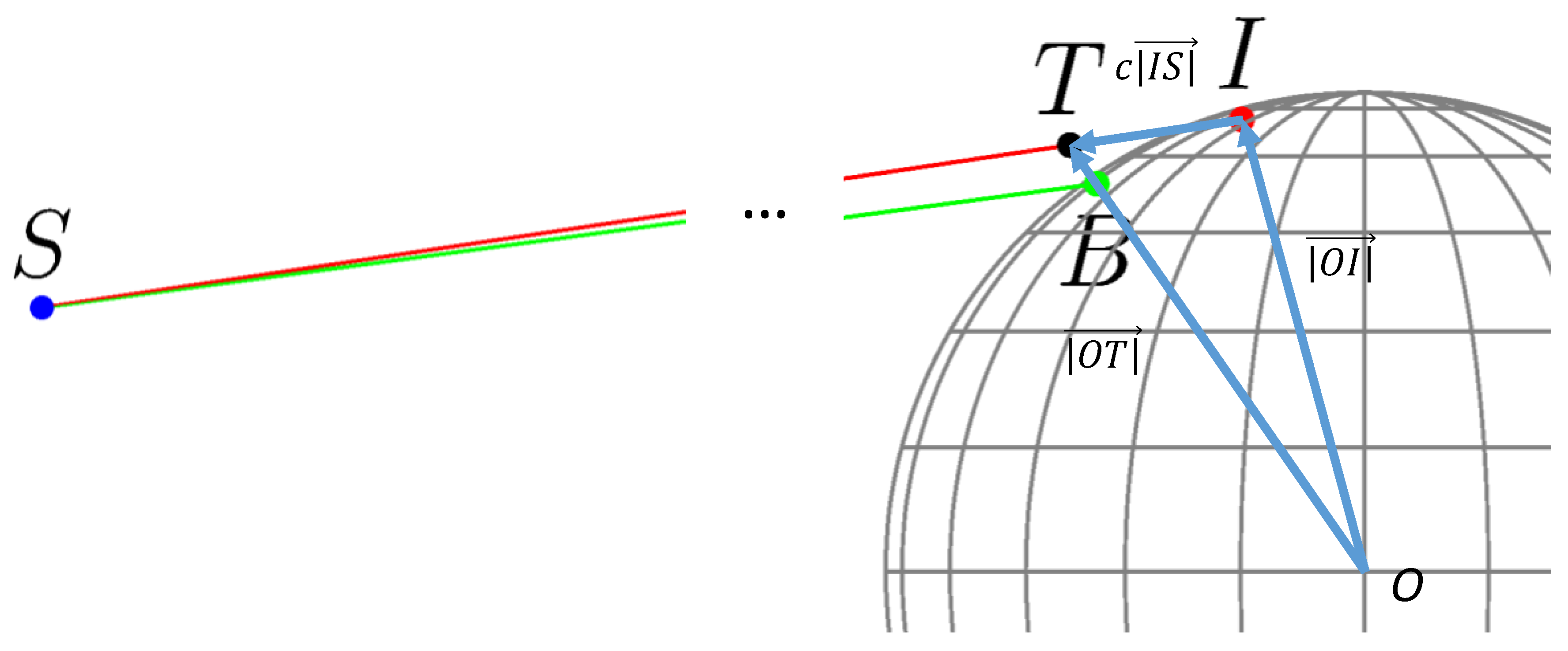
Parallax shift problem. The violet surface represents an image obtained from a geostationary satellite. The cloud top (T) is observed by the satellite as T’ (on the violet surface). The result of the reprojection of point T’ to ellipsoidal coordinates is I, which is not true the location of the cloud. The true location of the cloud is denoted as B, and from the perspective of the satellite sensor is observed as B’ on the violet surface. The square (marked as 1) shows how parallax shift affects the satellite image, where T’ is an image of the cloud top and B’ is where the cloud top should be placed according to its geodetic coordinates. The scale of the cloud height is not preserved.
Figure 1.
Parallax shift problem. The violet surface represents an image obtained from a geostationary satellite. The cloud top (T) is observed by the satellite as T’ (on the violet surface). The result of the reprojection of point T’ to ellipsoidal coordinates is I, which is not true the location of the cloud. The true location of the cloud is denoted as B, and from the perspective of the satellite sensor is observed as B’ on the violet surface. The square (marked as 1) shows how parallax shift affects the satellite image, where T’ is an image of the cloud top and B’ is where the cloud top should be placed according to its geodetic coordinates. The scale of the cloud height is not preserved.

Figure 2.
Three types of latitude: where is the geodetic latitude, is the geocentric latitude, is the parametric latitude, P is the point of interest on the ellipsoid, and P* is the image of the point of interest on a sphere. Based on figures from [23,24].

Figure 3.
Error in pixels caused by cloud height parallax effect for 5 chosen cites, assuming the observation is acquired by SEVIRI instrument at longitude of 0°. Spatial resolution was assumed as 3 km/pixel.
Figure 3.
Error in pixels caused by cloud height parallax effect for 5 chosen cites, assuming the observation is acquired by SEVIRI instrument at longitude of 0°. Spatial resolution was assumed as 3 km/pixel.

Figure 4.
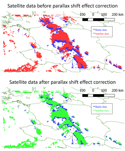
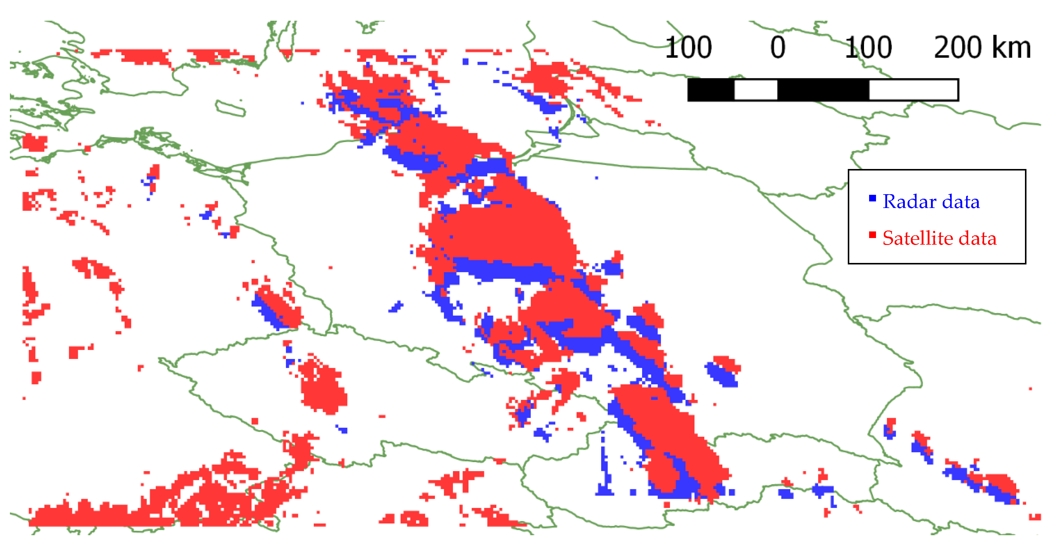
Comparison of detected precipitation mask based on ground-based radar data (blue) and data from Meteosat Second Generation (red). A parallax shift is particularly visible for small storm clouds in the bottom-right corner. The height of the cloud tops reaches 12 km. The stormy event is dated July 24, 2015, 13:00 UTC. EuroGeographics was used for the administrative boundaries.
Figure 4.
Comparison of detected precipitation mask based on ground-based radar data (blue) and data from Meteosat Second Generation (red). A parallax shift is particularly visible for small storm clouds in the bottom-right corner. The height of the cloud tops reaches 12 km. The stormy event is dated July 24, 2015, 13:00 UTC. EuroGeographics was used for the administrative boundaries.

Figure 5.
Vector notation in the Vicente et al./Koenig method.

Figure 6.
Comparison of detected precipitation mask based on ground-based radar data (blue) and data from Meteosat Second Generation with applied parallax correction using a numerical algorithm (green). Images of small storm clouds from satellite and meteorological radars in the bottom-right corner seem to overlap. The height of the cloud tops reaches 12 km. The stormy event is dated July 25, 2015, 13:00 UTC. EuroGeographics was used for the administrative boundaries.

Figure 7.
Maps showing error for the Vicente et al./Koenig (a,c,e,g,i) method and its augmented version (b,d,f,h,j) for several chosen cloud heights. Error are given in meters for the geostationary satellite coordinate system. NaN values for in-scope regions occur where the algorithm failed to calculate a solution. For each map, the median (med.) error was calculated.

Figure 8.
Error histograms for the Vicente et al./Koenig method (a,c,e,g,i) and its augmented version (b,d,f,h,j) for several chosen cloud heights. The Y-axis represents a count of 1 degree pixels, and the X-axis is the error in meters for the geostationary satellite coordinate system.
Figure 8.
Error histograms for the Vicente et al./Koenig method (a,c,e,g,i) and its augmented version (b,d,f,h,j) for several chosen cloud heights. The Y-axis represents a count of 1 degree pixels, and the X-axis is the error in meters for the geostationary satellite coordinate system.

Figure 9.
Maps with error (a,c,e,g,i) and number of iterations (b,d,f,h,j) for geodetic coordinates numerical algorithm (Geod. num. alg.) for several chosen cloud heights. Errors are given in meters for the geostationary satellite coordinate system. For each case, the median (med.) error was calculated.

Figure 10.
Histograms of error (a,c,e,g,i) and number of iterations (b,d,f,h,j) for geodetic coordinates algorithm (Geod. num. alg.) method for several chosen cloud heights. Error is given in meters for the geostationary satellite coordinate system.
Figure 10.
Histograms of error (a,c,e,g,i) and number of iterations (b,d,f,h,j) for geodetic coordinates algorithm (Geod. num. alg.) method for several chosen cloud heights. Error is given in meters for the geostationary satellite coordinate system.

Figure 11.
Scatterplot representing the dependence of radar reflectance and cloud optical thickness (logarithm) data for a stormy event on July 25, 2015, 13:00 UTC, without parallax effect correction (see Figure 4). The calculated Pearson’s correlation coefficient is 0.556.
Figure 11.
Scatterplot representing the dependence of radar reflectance and cloud optical thickness (logarithm) data for a stormy event on July 25, 2015, 13:00 UTC, without parallax effect correction (see Figure 4). The calculated Pearson’s correlation coefficient is 0.556.

Figure 12.
Scatterplot representing the dependence of radar reflectance and cloud optical thickness (logarithm) for a stormy event on July 25, 2015, 13:00 UTC, with parallax effect correction (see Figure 6). The calculated Pearson’s correlation coefficient is 0.683.
Figure 12.
Scatterplot representing the dependence of radar reflectance and cloud optical thickness (logarithm) for a stormy event on July 25, 2015, 13:00 UTC, with parallax effect correction (see Figure 6). The calculated Pearson’s correlation coefficient is 0.683.


Table 1.
The displacement function sensitivity in respect to h for five chosen cities for the geostationary sensor at longitude 0°. (N – North, S – South, E – East, W - West).
Table 1.
The displacement function sensitivity in respect to h for five chosen cities for the geostationary sensor at longitude 0°. (N – North, S – South, E – East, W - West).
| City | Geodetic Coordinates | Displacement Sensitivity as in Equation (32) |
|---|---|---|
| Cape Town | 33.9253° S 18.4239° E | 0.667 |
| Madrid | 40.4177° N 3.6947° W | 0.696 |
| Brasília | 15.7839° S 47.9142° W | 0.784 |
| Gdańsk | 54.3475° N 18.6453° E | 0.827 |
| Tromsø | 69.6667° N 18.9333° E | 0.868 |
© 2020 by the author. Licensee MDPI, Basel, Switzerland. This article is an open access article distributed under the terms and conditions of the Creative Commons Attribution (CC BY) license (http://creativecommons.org/licenses/by/4.0/).
Share and Cite
MDPI and ACS Style
Bieliński, T. A Parallax Shift Effect Correction Based on Cloud Height for Geostationary Satellites and Radar Observations. Remote Sens. 2020, 12, 365. https://doi.org/10.3390/rs12030365
AMA Style
Bieliński T. A Parallax Shift Effect Correction Based on Cloud Height for Geostationary Satellites and Radar Observations. Remote Sensing. 2020; 12(3):365. https://doi.org/10.3390/rs12030365
Chicago/Turabian StyleBieliński, Tomasz. 2020. "A Parallax Shift Effect Correction Based on Cloud Height for Geostationary Satellites and Radar Observations" Remote Sensing 12, no. 3: 365. https://doi.org/10.3390/rs12030365
Note that from the first issue of 2016, this journal uses article numbers instead of page numbers. See further details here.