Detecting Patterns of Vegetation Gradual Changes (2001–2017) in Shiyang River Basin, Based on a Novel Framework


1
College of Earth and Environment Sciences, Lanzhou University, Lanzhou 730000, China
2
The Key Laboratory of Western China’s Environmental Systems, Ministry of Education (MOE), Lanzhou 730000, China
*
Author to whom correspondence should be addressed.
Remote Sens. 2019, 11(21), 2475; https://doi.org/10.3390/rs11212475
Submission received: 10 September 2019
/
Revised: 18 October 2019
/
Accepted: 22 October 2019
/
Published: 24 October 2019
(This article belongs to the Special Issue Remote Sensing of Vegetation Dynamics and Resilience)
Abstract
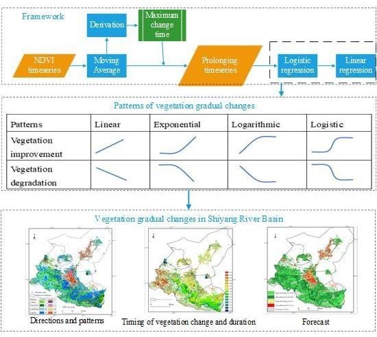
:A lot of timeseries satellite products have been well documented in exploring changes in ecosystems. However, algorithms allowing for measuring the directions, magnitudes, and timing of vegetation change, evaluating the major driving factors, and eventually predicting the future trends are still insufficient. A novel framework focusing on addressing this problem was proposed in this study according to the temporal trajectory of Normalized Difference Vegetation Index (NDVI) timeseries of Moderate Resolution Imaging Spectroradiometer (MODIS). It divided the inter-annual changes in vegetation into four patterns: linear, exponential, logarithmic, and logistic. All the three non-linear patterns were differentiated automatically by fitting a logistic function with prolonged NDVI timeseries. Finally, features of vegetation changes including where, when and how, were evaluated by the parameters in the logistic function. Our results showed that 87.39% of vegetation covered areas (maximum mean growing season NDVI in the 17 years not less than 0.2) in the Shiyng River basin experienced significant changes during 2001–2017. The linear pattern, exponential pattern, logarithmic pattern, and logistic pattern accounted for 36.53%, 20.16%, 15.42%, and 15.27%, respectively. Increasing trends were dominant in all the patterns. The spatial distribution in both the patterns and the transition years at which vegetation gains/losses began or ended is of high consistency. The main years of transition for the exponential increasing pattern, the logarithmic increasing pattern, and the logarithmic increasing pattern were 2008–2011, 2003–2004, and 2009–2010, respectively. The period of 2006–2008 was the foremost period that NDVIs started to decline in Liangzhou Oasis and Minqin Oasis where almost all the decreasing patterns were concentrated. Potential disturbances of vegetation gradual changes in the basin are refer to as urbanization, expansion or reduction of agricultural oases, as well as measures in ecological projects, such as greenhouses building, afforestation, grazing prohibition, etc.
1. Introduction
Satellite remote sensing has long been a technique of repeated temporal sampling on the earth’s surface. Currently, a large body of sensors provides continuous observations at various spatial, temporal and spectral scales over decades. Compared with change-detection based on bi/multi-date imagery which focuses on comparing just a few scenes [1], timeseries products cover landscape change processes during the whole observation period, change-detections based on timeseries are scene independent and possess significant potential for capturing more subtle changes caused by climatic variations, various human activities, or a combination of both [2]. Furthermore, the disturbance events in timeseries could be accurately localized in time. Therefore, they are receiving increasing attention for monitoring vegetation dynamics at global or regional scale.
Changes in ecological systems were divided into two types: gradual change and abrupt change [3], which refer to the trend component in timeseries beyond seasonal variations [4]. Recently, researchers are of particularly interest to detect abrupt changes caused by weather extremes, floods, fires, deforestation or pest outbreaks [5,6,7]. However, all ecosystems expose in the gradual change which is a slowly acting environmental process, e.g., climatic changes, land management practices or land degradations and restoration form severe disasters [8]. Furthermore, processes of gradual changes are never linear with time in a smooth way and even may be interrupted by sudden drastic trend breaks and then stall or reverse completely [9]. Therefore, exploring and extracting essential information characterizing vegetation gradual changes based on long-term remote sensing timeseries remains a large challenge.
Many approaches have been firmly established to characterize the gradual changes in vegetation. Trend analyses, e.g., linear regression based on Ordinary Least Squares (OLS), non-parametric Mann Kendall test and Theil-Sen estimator, are widely used methods by integrating bi-monthly observations for a whole year/growing season into yearly values (mean/sum/maximum) [10,11,12]. Trend analyses are simplification with explicit meanings: the slope values indicate the directions and rates of vegetation changes over time. However, vegetation may experience different short-term changes in long-term timeseries which may fail to be detected or completely be obscured in trend analyses [8,13,14]. Therefore, many new approaches were developed recently. Landsat-based Detection of Trends in Disturbance and Recovery (LandTrendr) [15,16] could detect changes by using a segmentation algorithm. However, it is specifically designed for Landsat datasets and had been proved unsuitable for other datasets [17]. Although a few parameters need to be set artificially, Detecting Breakpoints and Estimating Segments in Trend (DBEST) could also generalize main features in vegetation dynamics by applying a segmentation algorithm [18]. In addition, trend components in timeseries obtained by methods of Seasonal decomposition of Timeseries by Loess (STL) [19], Wavelet Transform (WT) [20] or Breaks For Additive Seasonal and Trend (BFAST) [21], could quantify inter-annual gradual changes in vegetation after being linear or piecewise linear modelled [5,6]. However, the trend components are incompetent at generalizing patterns of vegetation gradual changes because there are different number of break points in different pixels, which make comparisons between areas/pixels difficult.
The temporal trajectory-based detection method provides a flexible means to track changes for successive growing seasons or years. It was interpreted as a supervised change detection method [21] because it required a hypothetical temporal profile for timeseries based on the distinctive temporal progressions both before and after the disturbance event [22]. If the observed trajectory matches well with the curve of hypothesized trajectory, vegetation experiences the same change that hypothesized trajectory defined. Lambin and Strahler [23] detected and categorized the inter-annual change patterns of vegetation in west Africa by using trajectories of NDVI datasets of Advanced Very High Resolution Radiometer (AVHRR). Kennedy et al. [22] fitted temporal trajectories with four hypothesized exponential models to find the best fitting functions for forest dynamics by adjusting these initial parameters. Jamali et al. [13] tested a polynomial fitting-based scheme to account for the non-linear changes in inter-annual vegetation observations. Qiu et al. [24] assessed the Three-North Shelter Forest Program in China through a novel framework which could characterize where, when, what and how vegetation change, by combining trend analysis and temporal similarity trajectory.
This study proposes a novel framework that could detect where, when and how vegetation change over time based on the temporal trajectory for successive years of remotely-sensed indicator (NDVI) derived from high temporal resolution data (MODIS). The framework is devised for exploring the underlying short-time trends in timeseries which may be associated with a disturbance event. It not only generalizes the processes of vegetation inter-annual changes in the Shiyang River Basin, northwestern China into several patterns but also determines when vegetation gradual changes took place by the parameters in the logistic function. In addition, the MODIS NDVI timeseries for each pixel was prolonged before being fitted by using the logistic function to characterize all the non-linear patterns in the framework. Reasons for vegetation changes in the basin will be further determined by field investigations in combination with both the detected patterns and the timing of vegetation changes. The objective of this paper is to (1) develop a new framework to characterize the monotonic processes of vegetation gradual changes, (2) identify the patterns, trends, and timing of vegetation gradual changes in the Shiyang River Basin.
2. Materials
2.1. Study Area
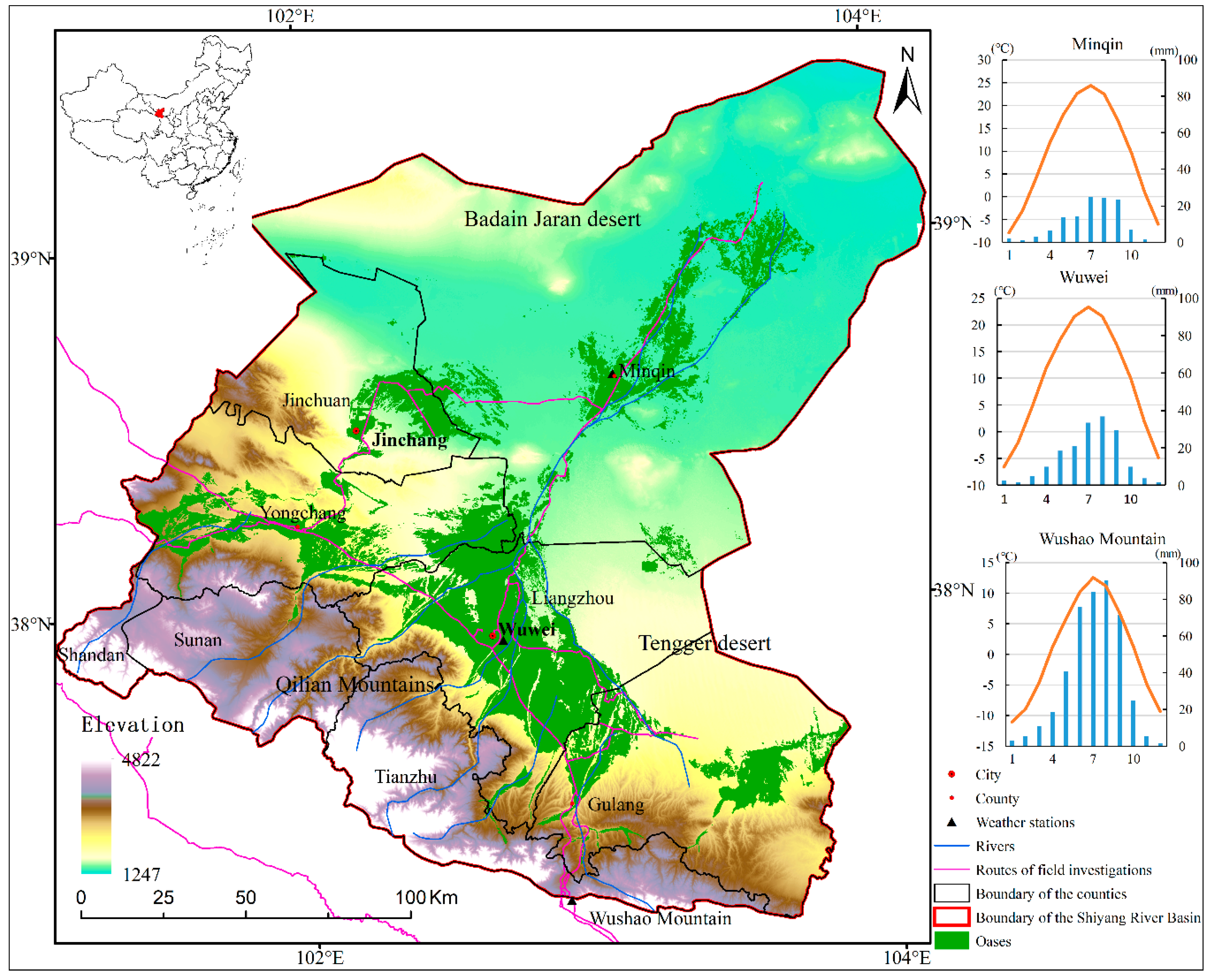
The study area is one of the three endorheic river basins in Gansu Province, northwestern China (36°45′–39°27′N, 101°08′–103°50′E) (Figure 1). Owing to the continuous uplift of the Qinghai-Tibet Plateau since the Pliocene, the Shiyang River Basin became a typical temperate continental climate characterized by long-cold winter, rare and irregular precipitation, and high evaporation. The annual mean temperature is around 7.7 ℃. Annual precipitation shows a seasonal distribution. About 90% of the precipitation takes place in the period from May to October. Precipitation reduces gradually from the south to the north. The altitudes in the basin range from 1247 m to 4822 m above mean sea level. Both the climate and the landscapes in the basin show obvious zonality due to the altitudinal gradient.
The southern part is the Qilian Mountains, which has a colder semi-arid to semi-humid climate with annual precipitation 300–600 mm [26]. Vegetation covers alternate regularly from desert steppe (1800–2300 m), scrub (2300–2800 m), forest (2500–3200 m), meadow (3200–4200 m) to glacier summit. Picea crassifolia and Sabina przewalskii are the representative plants in the forest region [27]. The dominant species of shrub are Potentilla fruticose, Caragana jubata, and Salix gilashanica. The main herbs are Cares atrata, Polygonum viviparum, and Carex lanceolate. Vegetation in the Qilian Mountains plays a critical role in water conservation and runoff formation. However, a lot of them were reclaimed for crop production in the last decades of the 20st century. The northern part is dominant by typical temperate continental arid climate with an annual precipitation less than 300 mm while annual potential evaporation more than 2000 mm. The annual precipitation is less than 50 mm in the northernmost places that are surrounded by Badain Jaran Desert and Tengger Desert. Drought-resistant, salt-resistant shrub and perennial sand-loving herbaceous plants, such as Nitraria sibirica, Salsola passerine, Eriocaulon truncatum Ham, Reaumuria soongorica Pall. maxim, Peganum harmala, Artemisia arenaria, and Agriophyllum squarrosum are the native vegetation in this region [28]. Wetlands along rivers (or floodplain), were reclaimed for crop productions as early as Han Dynasty (2000 years ago) [29]. Currently, they are agricultural oases with high productivities and well-developed irrigation networks consisted of rivers, reservoirs, canals, and wells. Spring wheat, barley, corn, and cotton are the staple crops. The Shiyang River originates from the Qilian Mountains and flows northeast to terminal Qingtu Lake and Baiting Lake. It is the main surface water for vegetation growth in the basin. Most of the water in the river is used for agricultural irrigation [28]. June to September is the flood season of the river, which is also the season for crop growth.
Human activities had caused severe natural vegetation degradations during the period 1950–2000 [28,30]. Since the beginning of the 21st Century, the Chinese government has invested a lot to restore the ecological ecosystem. A series of water reallocation projects were implemented to alleviate the shortage of water resources or tradeoff available water among different reaches, e.g., “Jingdian Water Diversion Project”, “Closing motor-Well and Reducing Cultivations”, “Key Governance Planning for the Shiyang River Basin” (KGPSRB) [31]. Other measures, such as grazing prohibition, rotational grazing, afforestation and returning farmland to grassland or forest, also brought positive outcomes [32]. In addition, the developments of the economy and society have greatly altered the styles of utilizations of nature resources. Vegetation dynamics in the Shiyang River Basin were remarkable over the past years, which makes it an ideal place to carry out the study.
2.2. Data Resources
MODIS, on board earth observation system terra satellite of the National Oceanographic and Atmospheric Administration (NOAA), crosses the dayside equator at 10:30 a.m. local time [33]. The 250 m 16-day composite MOD13Q1 (Collection 6) datasets were downloaded from the online Data Pool at NASA Land Processes Distributed Active Archive Center (LPDAAC) [34]. The datasets were implemented several major improvements due to a new calibration approach and were released in February 2015 [33]. The datasets contain a variable number of “Science Data Sets” (SDS) that include 16-day NDVI, EVI, and quality assessment (QA) [35].
MOD13Q1 datasets were available for the period from April 2000 to December 2017 in our study. Mosaic, resampling, and reprojection to Universal Transverse Mercator (zone 47) were done firstly by using the MODIS Reprojection Tool (MRT). Then, all the pixels with NDVI values greater than zero (waterbody, snow, glacier or bare land) and the VI usefulness score in QA band greater than four, were masked out. We finally obtained all vegetation covered pixels with good observations. Lastly, a simple linear interpolation method was done to fulfill the missing values in the NDVI timeseries for each pixel.
Monthly NDVI values from January 2001 to December 2017 were produced by a maximum synthesis of the two-phase data. We calculated the mean value from May to September for each year and considered it as annual mean growing season NDVI which represented the overall state of vegetation growth expecting to reduce influences of anomalous events, e.g., rainstorm or flood. We finally obtained timeseries datasets that consisted of 17 growing seasons NDVIs. Since sparse vegetation or desert vegetation is deeply influenced by fluctuations from precipitation in arid and semi-arid regions, only pixels with maximum annual mean growing season NDVI (NDVImax) in the 17 years not less than 0.2 will be discussed in our study.
3. Methods
3.1. The Overview of Our Framework
Vegetation will keep in a stable state or slowly changing over time. Once disturbed, vegetation will change rapidly and shift to another state until a higher or lower equilibrium is reached [9]. Therefore, the processes of vegetation gradual changes within a certain period (2001–2017) in our study are divided into four patterns based on the time and durations of the disturbance event. They are ongoing change, stable in the early stage and keep changing later, continuously changing in the early stage and then stable, change from equilibrium to a new equilibrium, which are named linear pattern, exponential pattern, logarithmic pattern, and logistic pattern, respectively (Table 1). All patterns are further binned into two types, consisting of either positive or negative trends. Other non-monotonic patterns, such as the pattern like increase and then decrease (or decrease, then increase), are not discussed in the framework.
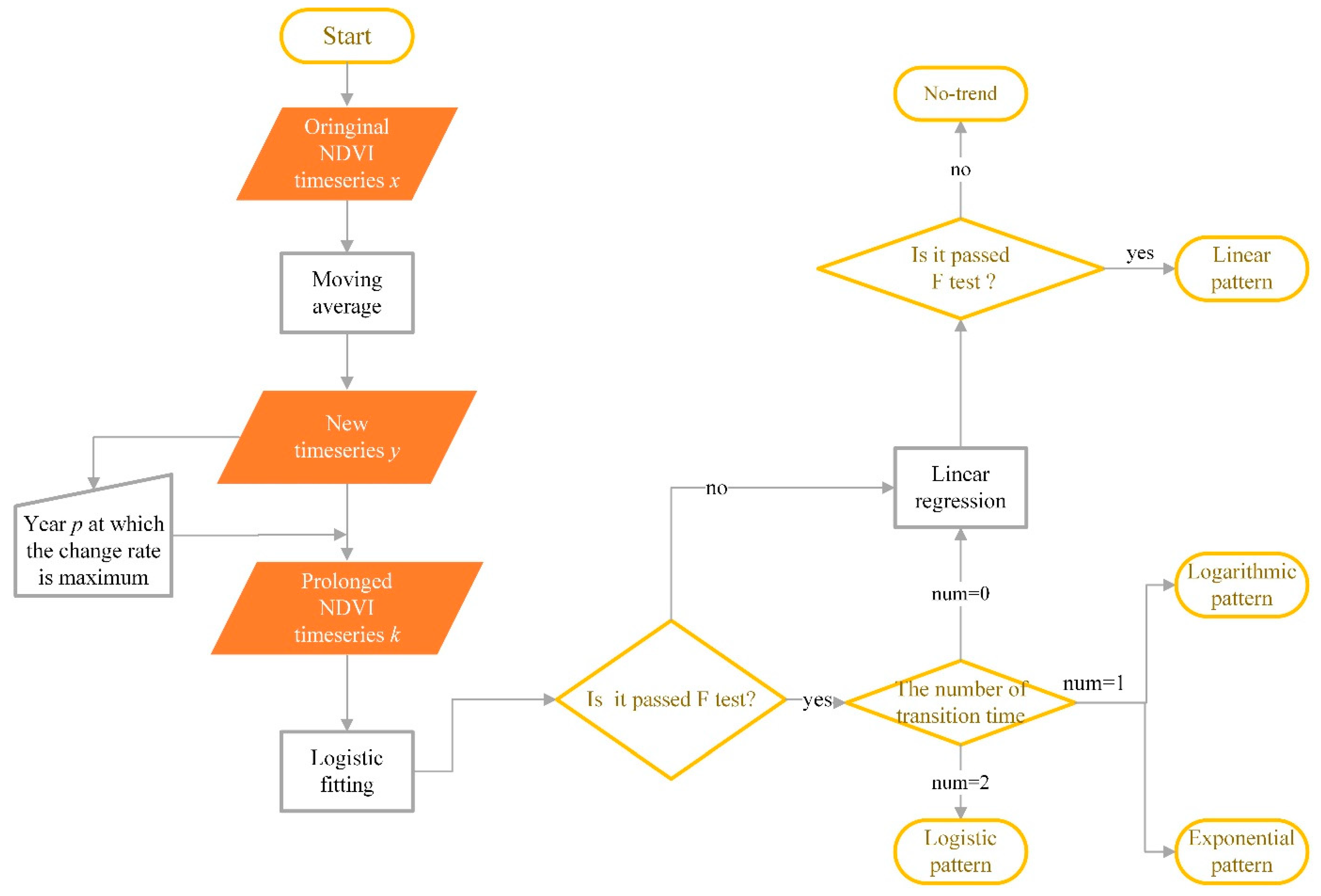
Generally, each parameter in the logistical function has a ready ecological interpretation. An S-type curve of logistic function could seem to be a combination of exponential curve and succedent logarithmic curve. Therefore, a logistic mathematical model with four parameters is chosen as the main fitting function in our framework. In order to fit the patterns using a logistic function, modified operations on original NDVI timeseries must be done first. The overall flowchart is shown in Figure 2. All the procedures are implemented using MATLAB (R2016b) software.
3.2. The Procedures of Our Framework
3.2.1. Noise Smooth by Using Moving Average
The smooth treatment is expected to reduce the influences of likely outliers in timeseries which may be caused by agriculture planting adjustments, inter-annual fluctuations of precipitation or other factors. A moving average (MA) is the commonly used smooth method, which could eliminate the seasonal and individual irregular changes, and highlight the long-term trend in timeseries. Specifically, for a timeseries x with n observations (n = 17 in our study), a single moving average in the forward and backward directions is calculated at every time point .
Then, a new timeseries y for each pixel is obtained.
3.2.2. Modeling All Non-Linear Patterns Using a Logistic Function
We model all non-linear patterns using a logistic function based on two core premises: (1) If vegetation growth is interfered, it will shift to an alternative state of rapid change. There must be a time p that the change rate in vegetation is maximum. The time p is consistent with the timepoint in the temporal profile of NDVI timeseries at which the slope value is maximum. (2) In order to present non-linear patterns, the smoothed NDVI timeseries y is prolonged by centering on p before applying to the logistic regression. The prolonged elements are filled by the first or last item of timeseries y. The concrete procedures are presented as follows:
(1) Identifying the Timepoint P
The differences of the forward and backward directions in timeseries y are calculated at every timepoint as follows:
The year corresponding to the maximum absolute is the timepoint p.
(2) Prolonging Timeseries Y
The length of prolonged timeseries is symmetric about p. Therefore, the length of the prolonged timeseries (L) for each pixel is calculated as follows:
where if p is equal to 9, the prolonged timeseries k is the original timeseries y. If p is greater than 9, the first 17 elements in prolonged timeseries k are original timeseries y, and others are supplemented by the last element in timeseries y. If p is less than 9, the last 17 elements in k are identical with y, and others are supplemented by the first element in timeseries y. Finally, new timeseries k which contains the whole timeseries y is obtained.
(3) Modeling the Prolonged Timeseries K Using a Logistic Function
We fit the prolonged timeseries k by a logistic function. The function is shown as follows:
where t are the serial numbers in timeseries k which range from 1 to L, f(t) are the values in the prolonged NDVI timeseries k, parameter a represents the change magnitude of NDVI over a period, the symbol of b denotes the direction of vegetation change, c is the location where the fitting value is equal to (a+d)/2 and parameter d reveals the initial background NDVI value. The goodness-of-fitting is implemented by the standard F statistics test. Only the goodness-of-fitting of the part corresponding to the period 2001–2017, are taken into consideration in our study.
(4) Distinguishing Non-Linear Patterns According to the Number of Transition Years
The curvature (K) for the logistic function is computed first using the following equation:
where . a, b, c, are the parameters in Equation (4).
The transition year refers to the time at which vegetation gain/loss begins or ends. The beginning or stopping of vegetation change is attributed to a disturbance event or reaching a steady state. We define the transition years as the timepoints at which the change rate of curvature (K’) in the logistic curve exhibits maximum or minimum. More information could refer to literature of Zhang et al. [36]. Specifically, if b is lower than zero, the locations of the two positive extreme values of K’ are the transition years, if b is greater than zero, the locations of two negative extreme values of K’ are the transition years. It is worth noting that we only concern the number and locations of the transition years in the period corresponding to years from 2001 to 2017. All the non-linear patterns are then distinguished by the number of transition times. If the number is 2, we conclude that vegetation change follows an S-type curve, while if the number is 1, vegetation change process is considered as exponential pattern or logarithmic pattern. Both patterns could further be differentiated by comparing the transition year to the parameter c in Equation (5). If the transition time is prior to c, the pattern is exponential, otherwise, it is logarithmic.
3.2.3. Identifying Linear Pattern of Vegetation Gradual Change
Linear regression of NDVI timeseries y against time is implemented to the pixels which do not pass the F statistics test in logistic fitting and pixels without transition year. The formula as below:
The parameters are estimated based on OLS:
Where i is the ith year in timeseries y, s, and slope are the parameters in linear regression, slope denotes the changing trend in vegetation, n is the length of timeseries y, is the NDVI value in the ith year. The goodness-of-fitting is also implemented by adopting the standard F-test. If pixels pass F-test, we assume that vegetation growth in the pixels experience linear changes. The remaining pixels which do not belong to the aforementioned patterns are defined as no-trend.
3.3. Method for Validation
Field validation of year-to-year changes is often not straightforward due to a lack of consistent observation spanning two decades at a large spatial scale [22]. Fortunately, vegetation dynamics are closely related to landscape transformations or modifications caused by disturbance events [37,38]. Therefore, pattern of vegetation gradual changes obtained from our framework was evaluated by exploring its sensitivity to landscape transformations/modifications. Site validation and regional validation are combined to assess the performance of our framework in characterizing the temporal trajectory of vegetation gradual changes. If the shape of the curve in each site/region was consistent well with the process of land cover change disturbed by the known fact, and the observed transition years in the curve was consistent with the timing of the known fact, we assumed that the framework is effective in characterizing vegetation gradual changes. The known facts which led to significant landscape transformations or modifications were obtained from field investigations conducted from July to October in 2018 (Figure 1). Most of them were further confirmed by the almost yearly high-resolution images on Google Earth Pro (version 7.3) and reports in newspaper or existing literature. It is worth noting that both the sites and the regions for validation were selected randomly from the areas where the same patterns concentrated. They are shown in Figure 3.
4. Results
4.1. Patterns of Vegetation Gradual Changes in the Shiyang River Basin
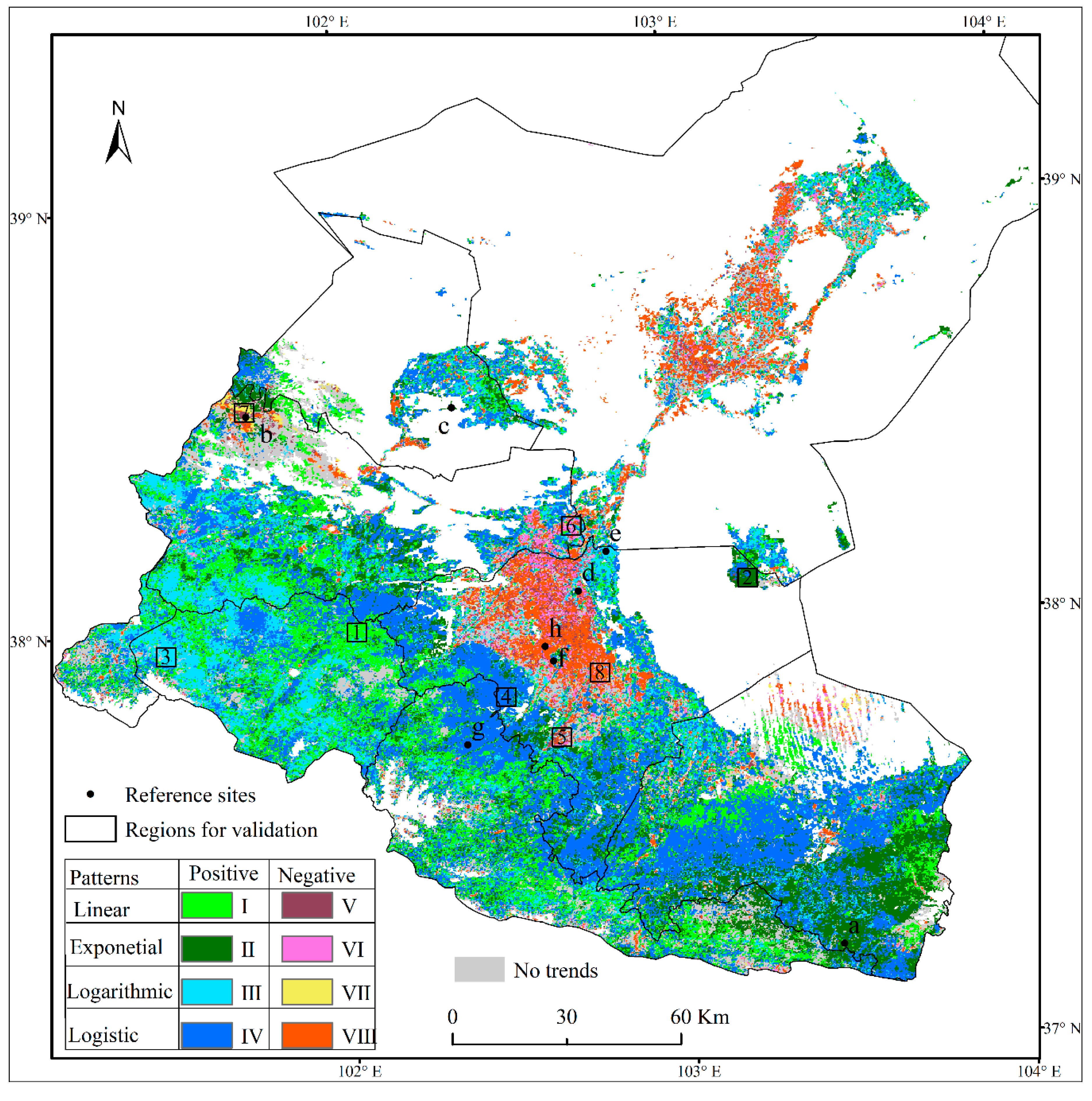
Patterns of vegetation gradual changes in the Shiyang River Basin are shown in Figure 3. 87.39% of vegetation (NDVImax ≥ 0.2) changes were significant which had passed the F test (P < 0.05). The most widespread pattern was logistic (36.53%) (Table 2). Linear patterns made up 20.16% of the entire vegetation covered areas, of which 18.43% were increasing while 1.73% were decreasing. Exponential and logarithmic patterns involved 15.42% and 15.27%, respectively. Most of them possessed increasing trends, while only about 1.88% and 0.79% had trends with negative slopes, respectively.
For the pixels with significantly changes, 87.57% were positive while only 12.43% were negative. Greening (Types I-IV in Figure 3) was universal in the basin and dominant in all patterns (Table 2). Vegetation improvements mainly located in the Qilian Mountains, Yongchang County, Jinchuan Oasis, the transition zones between Liangzhou Oasis and deserts, and the north of Minqin Oasis. Specifically, linear greening areas widely distributed in the higher altitudes of the Qilian Mountains (2300–3200 m) where the forest is the main landscape, while the logistic increasing patterns widely distributed in the lower altitudes of the Qilian Mountains where the steppe and barren arable lands are the main landscapes. The exponential increasing pattern was dominant in the east of the Qilian Mountains while the logarithmic increasing pattern was dominant in the west of the Qilian Mountains. Oasis areas in Jinchuan County and Yongchang County and the southern edge of liangzhou Oasis experienced a logistic increasing process. The greening patterns in the north of Minqin Oasis are complex. Almost all the decreasing NDVI trends (Types V-VIII in Figure 3) concentrated in the interior of Liangzhou Oasis, Minqin Oasis, and highlands in the north of Yongchang County. 59.56% of the decreasing patterns are logistic which were mainly concentrated in areas near cities or towns. The exponential decreasing patterns concentrated in the oasis areas farther from the cities. The logarithmic decreasing pattern was rare and largely constrained in the highlands in the north of Yongchang County.
4.2. Transition Years and Durations of Vegetation Change
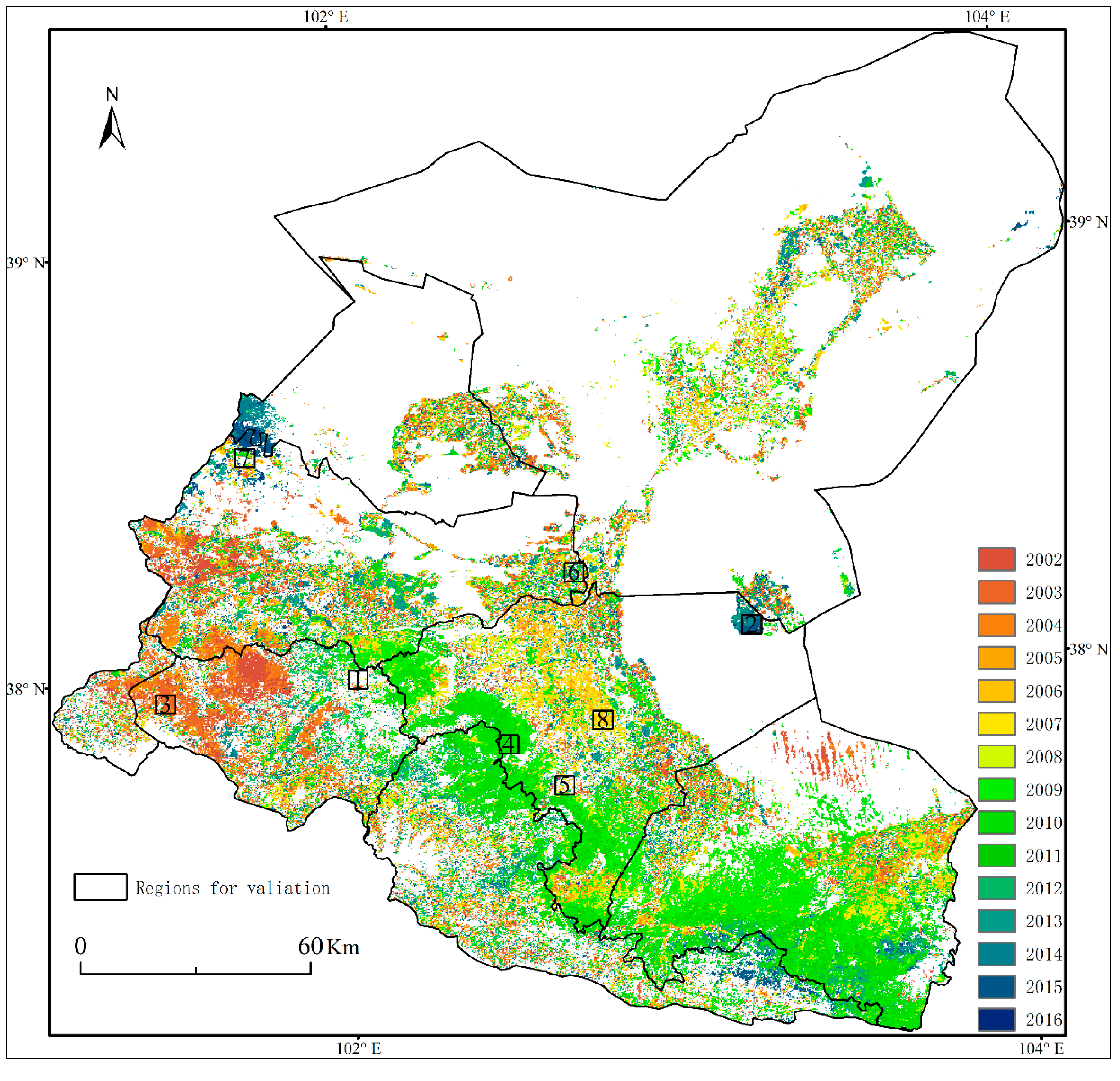
There is one transition year at which vegetation began or stopped to change in the exponential pattern and the logarithmic pattern (Table 1). There are two transition years in the logistic pattern. The transition years of the exponential pattern and the logarithmic pattern, and the first transition year of the logistic pattern are shown in Figure 4. The periods of 2008–2011, 2003–2004, and 2009–2010 were the main timeframes that vegetation changes took place in the exponential increasing pattern, the logarithmic increasing pattern and the logistic increasing pattern, respectively (Figure 5). 2006–2008 was the main transition period for all the decreasing patterns.
The spatial distribution of the patterns (Figure 3) and that of the transition years (Figure 4) shows a high consistency in many places. Specifically, vegetation in the west of the Qilian Mountains where possessed large areas of the logarithmic patterns kept improving in the early stage of the observation period and then maintained well growth conditions since 2003 or 2004. Vegetation gains of the exponential increasing pattern which were very common in the east of the Qilian Mountains and parts of Jinchuan Oasis started later than 2010. The steppes in the lower altitudes of the Qilian Mountains started to improve since 2009. In addition, vegetation improvements in the middle of Yongchang County and the reclaimed oases in the south of Tengger desert took place in the earlier years (before 2005) while that in the east of Yongchang County, the north of Minqin Oasis took place in the later years. NDVIs in most of Liangzhou Oasis and Minqin Oasis started to decline during the period 2006–2008, while NDVIs in the east of Yongchang County where the exponential decreasing pattern concentrated began to decline in 2010.
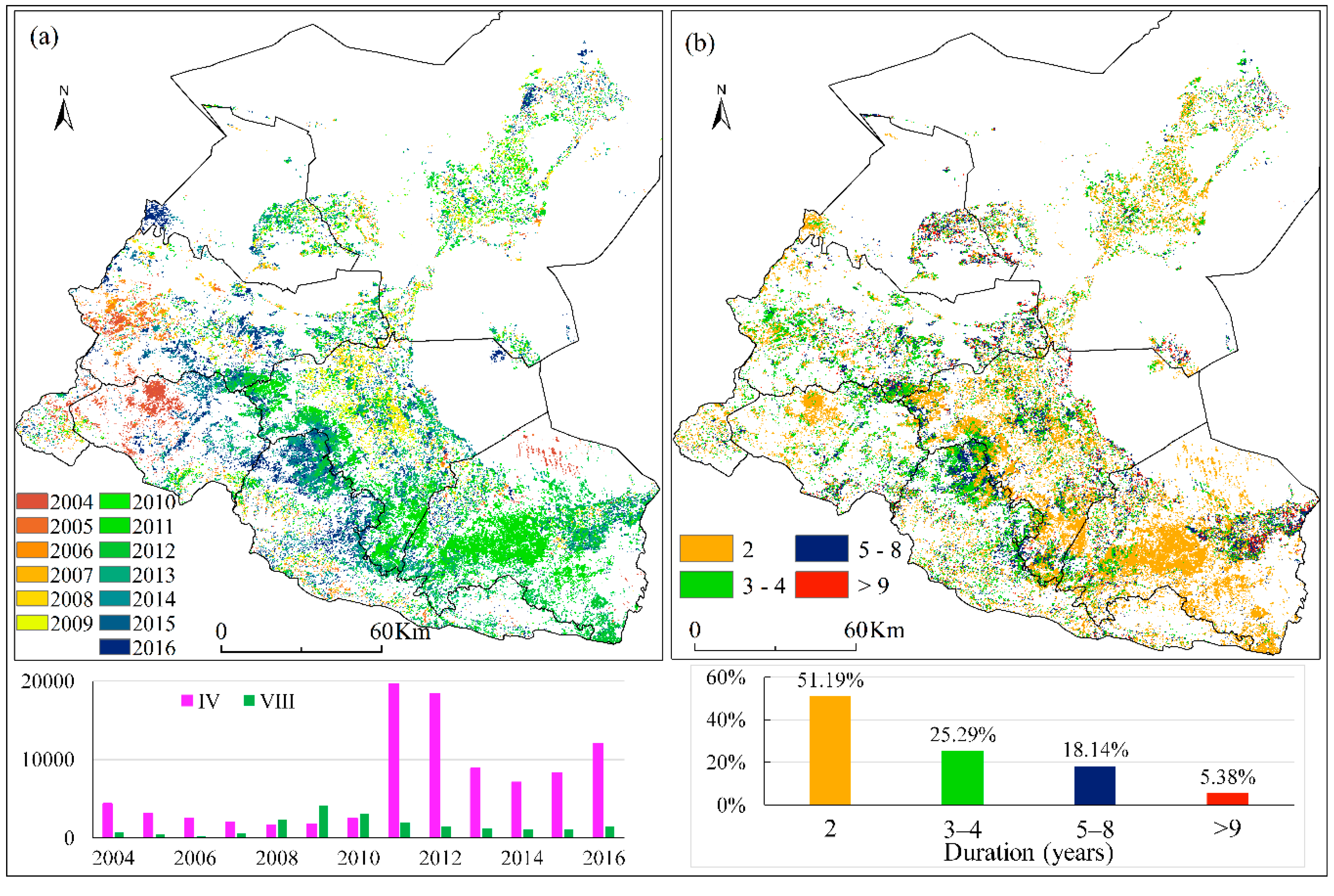
We discussed the transition years in the logistic pattern deeply because the logistic pattern accounted for a large proportion and had two transition years. The start years of vegetation changes in the logistic pattern had been descripted (Figure 4). The end years of vegetation changes in the logistic pattern are shown in Figure 6. As mentioned above, 2009–2010 was the main period (47.22%) that NDVIs of the logistic increasing patterns started to rise. However, most of the improvements stopped after 2011, mainly stopped in 2011 and 2012 (Figure 6. a and the histogram below a). 2006–2008 was the dominant period that NDVI began to decline, which accounted for 55.22% of the logistic decreased pixels. The NDVI decreasing trends stopped in 2009 or 2010. The duration of vegetation change for each pixel was calculated through subtracting the end year from the start year (Figure 6). More than half (51.19%) of logistic patterns possessed a continuous change interval of two years (Figure 6. b and histogram below b). The longer vegetation changes lasted, the smaller the proportion. 76.48% of vegetation changes in the logistic pattern lasted less than 4 years. Areas with a duration over 8 years (5.38%) were mainly concentrated in the continuously reclaimed agricultural oases [39].
4.3. Forecasting Vegetation Condition in the Shiyang River Basin
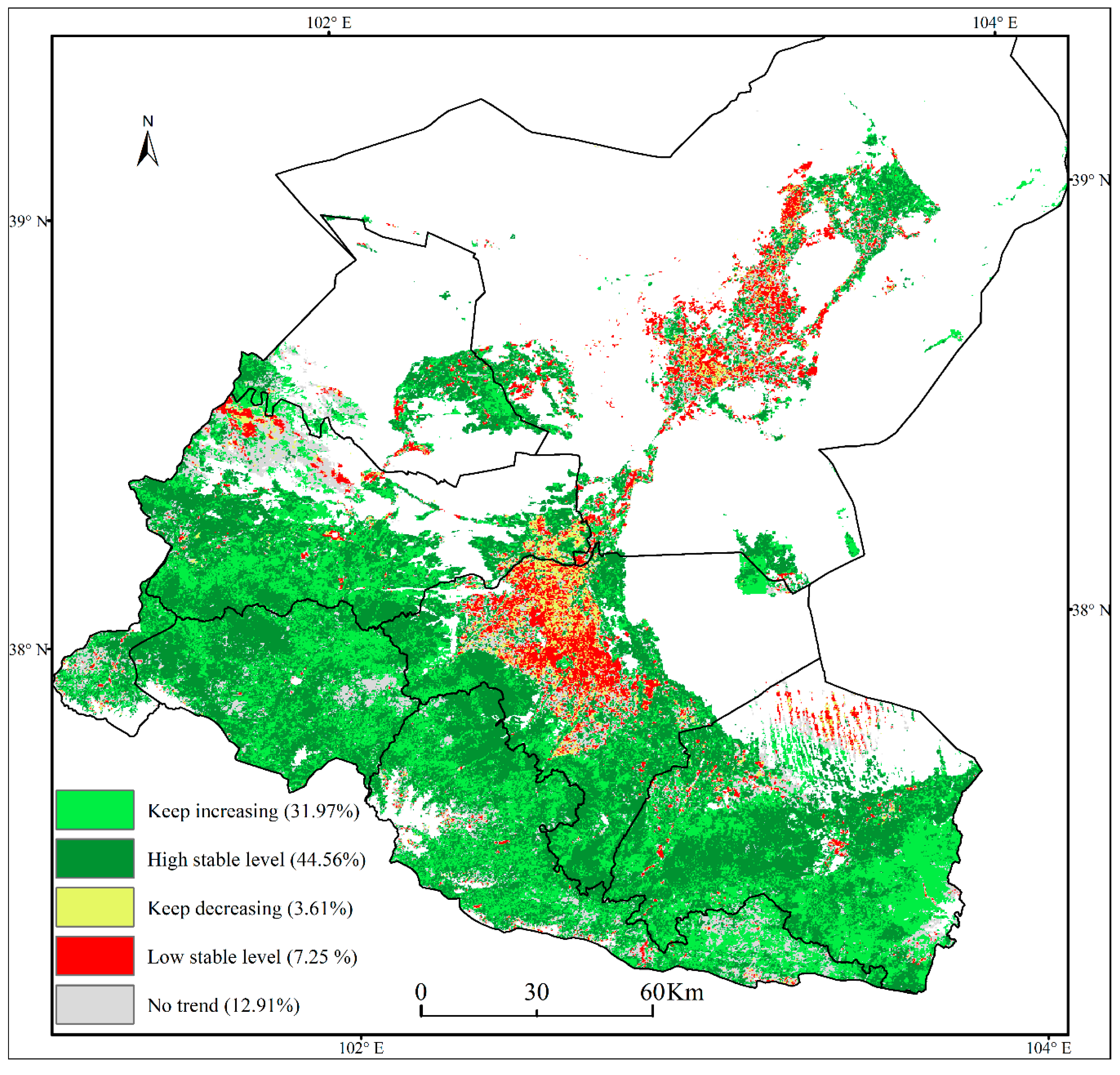
The forecast for vegetation changes in the near future are shown in Figure 7. Our forecasts are not predictions, but rather are estimates of vegetation gradual changes which should continue on the trajectories of the past years. Therefore, we forecasted vegetation changes in near future according to the shape of the curve of NDVI timeseries in Table 1. Except for a few (12.91%) of vegetation covered areas which have no significant trends, 44.56% of vegetation will be in a stable state of high-level equilibrium, 7.25% will be in a low-level equilibrium, 31.97% of vegetation in the basin will keep improving persistently along with the current directions, and NDVIs in 3.61% of vegetation covered areas will keep declining. Vegetation in the Shiyang River Basin is generally in or toward a benign condition. The ongoing greenings in the high altitudes of the Qilian Mountains and Yongchang County are widespread. The continuously declining NDVIs mainly concentrated in the rural areas of Liangzhou oasis. More attention should be paid to find out reasons for the declined or declining NDVIs.
4.4. Results of Validation
The temporal profiles of the NDVI timeseries x, the smoothed timeseries y, and the prolonged timeseries k, the fitting functions and the locations of transition years for the eight selected reference sites are listed in Figure 8. The known fact of landscape transformation/modification in each site we obtained for validation is listed in Table 3. Specifically, the temporal trajectories in six sites of them were validated by subjectively comparing with the landscape transformations obtained from the images on Google Earth Pro. The Landscape modifications in the other two sites were identified by reports in the local newspaper. Our results indicate that the shape of the curve in every site coincide well with the processes of landscape changes obtained from field investigations, reports in newspaper, and higher resolution images on Google Earth Pro. Furthermore, a good agreement is also found between the detected transition years and the timing at which the landscape transformations or modifications took place in all the non-linear patterns.
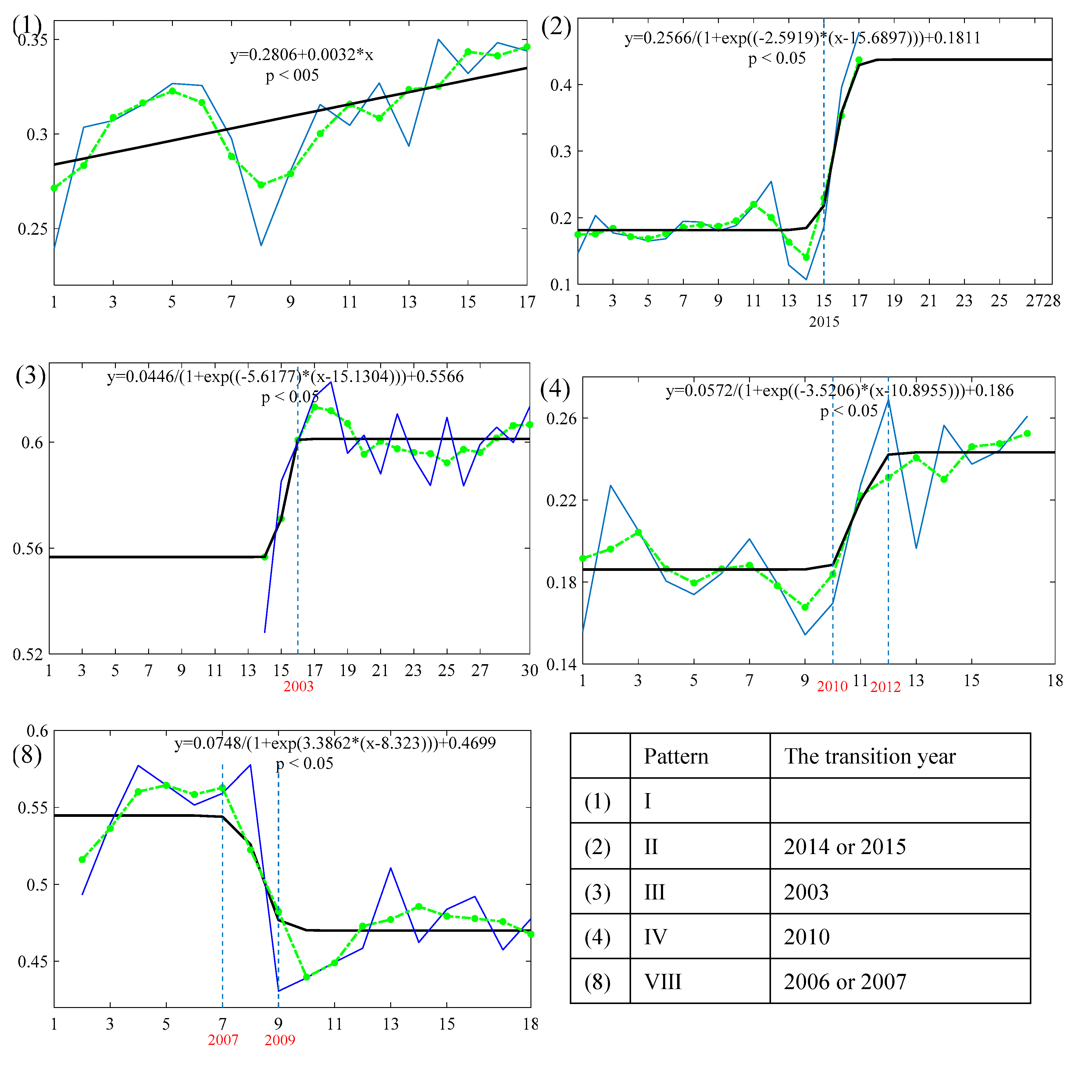
Eight regions (approximately 5 km × 5 km) for validation are presented in Figure 3. Almost all the pixels in each selected region have the same pattern which is dominant in the region and the same or similar transition year except that in Region 5, 6, 7. The three regions are the places where linear decreasing pattern, exponential decreasing pattern and logarithmic decreasing pattern were concentrated. However, the exponential decreasing pattern in Region 6 is not dominant and the transition years in Region 6 vary greatly (Figure 4). Similarities are also found in Region 5 and Region 7. Therefore, only the other five regions are discussed in precise details (Figure 9). We first calculated the annual mean NDVI of each region. The pixels involved in the calculation in each region must have the same transition years as that listed in the table of Figure 9. Then, the pattern and the transition years of the region were also detected by adopting our framework.
We found that both the patterns and the transition years detected on the regional scale are coincident with that detected on the pixel scale. Therefore, the accuracy of our framework was further assessed on a regional scale. “Three-North Shelter Forest Program (Fourth and Fifth periods)”, “Natural Forest Protection Project” and “Returning Farmland to Forest Project” were carried out successively in the Qilian Mountains before 2001. Tianzhu County has been committing to those projects over the past decades [42]. Logarithmic increasing patterns were found in the places where vegetation growths had been recovered completely and reached a high coverage [43]. Since the lower altitudinal limit of the forest belt in 1949 was 1900 m [44], linear increasing trends were common in most of the forest regions, like Region 1. Region 2 was reclaimed as large-scale farmland in 2014 or 2015, which we confirmed according to the yearly high-resolution images on Google Earth Pro. Agriculture oases are irrigated regularly, an increasing exponential pattern was detected in Region 2. The implementations of grassland restoration projects, such as “Natural Grassland Restoration and Construction Project” (2001–2005) and “Returning Pasture to Nature Grassland” in Sunan County, Zhangye Municipality were earlier than other places (about in 2010) in the Qilian Mountains [45]. The grasslands recovered from overgrazing and reached a high stable state in 2003. Therefore, vegetation growth in Region 3 experienced a logarithmic increasing process with an earlier transition year (2003). Pastures in Region 4 were returned to nature grasslands in 2010. Vegetation recovered from overgrazing quickly [41] and logistic pattern was detected in Region 4. KGPSRB, invested largely by Chinese government was carried out in years of 2006–2011 [46]. In order to increase runoff and reduce groundwater extraction in the downstream area, the traditional crop plantings were replaced by protected agriculture (sunglass/plastic greening house) and large areas of croplands in Minqin Oasis were abandoned. Region 8 in Qingshui Town is a demonstration area where a great deal of greenhouses built in 2006 or 2007.
5. Discussion
5.1. Strengths and Limitations of the Framework
Timeseries products present different temporal scales components, such as seasonal variations, long-term and short-term fluctuations [2]. Their high temporal resolution offers the opportunity to define time profiles of vegetation dynamics. Although many methods have been developed to explore vegetation dynamics at a global or regional scale, quantitative methods that could automatically address where, when and how vegetation change are still lacking [24]. Trajectory-based change detection is an inevitable choice to do this work by constructing a ‘curve’ or profile of full temporal records for each pixel. Nowadays, the method has been successfully applied in forest-related change analyses [47,48], land use classification [49,50], and cropland variations [51].
The framework we proposed in our study is a trajectory-based change detection method. It has several desirable properties compared with other fashionable methods. Firstly, unlike the widely used trend analyses which hypothesize that ecosystems/vegetation always change linearly in a direction, our framework could detect the non-linear change patterns in vegetation. All patterns in the framework can be interpreted from unambiguous biophysical standpoints. Secondly, unlike DBEST and BFAST [18], our framework automatically generalizes processes of vegetation gradual changes into different patterns without setting any parameters. Furthermore, the patterns between different pixels or areas could be compared easily. Although DBEST and BFAST could also track vegetation gradual change by a piecewise linear model on the pixel scale, the number of breakpoints must be set by users when the method was extended to the regional scale. For example, de Jong [8] detected the short-term greening or browning periods within long-term timeseries by dividing the trend component in BFAST into four segments which were separated by three breakpoints. Then, the duration of the significant greening and browning segments, the magnitude of change in NDVI, and the abrupt changes could be compared between pixels subsequently. Lastly, trajectory-based change detection only functions when the process of vegetation change matches well with the hypothesized trajectory. Temporal trajectories of vegetation changes in different pixels may be different. Therefore, many mathematical models are needed to fit the trajectories. However, just a logistic model is used to simulate all the non-linear monotonic patterns in our framework.
Drawbacks of our framework are obvious. Firstly, only four monotonic patterns and eight types are presented. All the patterns are associated with only one disturbance event within the timescales of the observation period (Figure 4). Generally, changes in vegetation are complicated and difficult to be generalized by a single function. Therefore, patterns that are composed of the general categories in our framework, or patterns that vegetation gradual changes were stalled or reverse by abrupt events, were not discussed in this study. New models that could detect both the monotonic and the non-monotonic patterns are needed to be induced in future. Secondly, the smoothed treatment implemented on the NDVI timeseries makes the framework unsuitable to detect subtle changes or abrupt changes [52]. However, it makes the framework unspecific to the MODIS timeseries products which do not suffer from the problem of data discontinuity. The data discontinuities which may be caused by changes in different sensors, orbital drift in the satellite overpass times, variations in sun-sensor-viewer geometry or differences in the atmospheric conditions (i.e., water vapour content, aerosols) [53] are common in other timeseries products, such as datasets from AVHRR, Landsat and VEGETATION.
5.2. Factors that Influence the Detected Patterns by Our Framework
Patterns of vegetation gradual changes are closely related to the regimes of the disturbances (intensity, time and duration) in our study. Our framework was designed based on the fact that the temporal trajectory of vegetation will alter after a major disturbance event. Therefore, the patterns of vegetation change largely depend on the regimes of the disturbance event. If the disturbance event priors to the observation period, vegetation growth may experience a logarithmic pattern or a linear pattern during the detected period. The exponential pattern or logistic pattern may be detected if the disturbance event is introduced in the midst of the observation period. The length of timeseries also affects the detected patterns. On one hand, a longer observation period means a more complicated pattern of vegetation dynamics, which our framework is incompetent to detect. Moreover, the longer the timeseries is, the more likely that this effect conceals actual short-term trends [8] and improves the power of the linear tread analysis [54]. On the other hand, if the observation period is short, or the duration of the disturbance event is long enough, vegetation changing condition may persist throughout the whole observation period. A linear pattern will also be detected. Finally, we found that the patterns of vegetation gradual changes are also influenced by the pre-existing land cover because the timescales over that the landscapes are affected by or recover from over exploitation are different. Compared with the forest ecosystem, grassland is more sensitive to disturbances [55]. It won’t take them a long time to reach a new equilibrium. Therefore, grasslands or sparse vegetation regions in the lower altitudes of the Qilian Mountains were mostly characterized by the logistic pattern while the forest areas in the higher altitudes of the Qilian Mountains are dominant by the linear patterns (Figure 3).
5.3. Validation Method
The basic problem in timeseries-based change detection is the assessment of the method [56]. A general lack of reliable temporal field-based datasets spanning the duration of the satellite time-series limits the quantitative evaluation of the change detection methods. Most of the studies have no field data to support their findings or have no reliable techniques to assess the statistical significance of the detection methods [2]. Field investigation is still the most commonly used method for verification. Fuller et al. [10] examined the results of linear trend analysis of NDVI images in light of harvest measurements conducted in Senegal’s rangelands and croplands. Qiu et al. [24] recently assessed the processes (dynamic patterns) of vegetation dynamics obtained by combination analysis of vegetation trends and temporal similarity trajectory through focusing on the primary and easily observable landscape changes. In addition, some researchers resorted to “validating” the trend analysis through the use of regional opinion or by invoking somewhat obliquely-related ancillary data sets and publications [54]. Since no independent datasets were available for validation, Kennedy et al. [22] tested the accuracy of a new trajectory-based method by comparing the detected changes with the direct interpreter delineation obtained from the timeseries images itself. Wessels [54] treated the simulation approach as an alternative avenue of field investigations to test the sensitivity of trend analyses (linear or non-parametric methods). We collected the evidence of vegetation gradual changes in the Shiyang River Basin in many ways, including field investigations, exiting publications and almost yearly higher resolution images on Google Earth Pro. The evidence of landscape transformations or modifications on both the pixel scale and the regional scale were used to evaluate the effectiveness of our framework.
5.4. Potential Driving Factors of Vegetation Gradual Changes
Our results demonstrated that vegetation in the Shiyang River Basin experienced significant changes during 2001–2017, and greening was widespread throughout the basin, which agrees with the recent research in this region [57]. Our study further indicated that human activities, especially various ecological restoration projects could explain a large part of gradual changes in the Shiyang River Basin because there is a good agreement between the detected patterns of vegetation changes and human-induced landscape transformations or modifications. Our results are consistent with that of Guan et al. [57] who also confirmed that vegetation changes in the east of the Qilian Mountains and oasis areas in the Hexi region, which is the Shiyang River Basin were mainly influenced by human activities.
Human activities refer to the expansion or reduction of agriculture oases, urbanization, migration and various measures in ecological restoration policy. The basin has stepped into a period of rapid urbanization after entering the 21st century. A large part of farmlands around the cities and towns had been transformed into urban areas, which caused significant logistic decreasing patterns during 2001–2017. Since there are obvious spatial differences in time at which agricultural oases expended [39], different increasing patterns were found in the newly reclaimed oases. The logarithmic increasing patterns were found in the north part of the transition zones between Liangzhou oasis and Tengger Desert (Site g in Figure 8), and the southern edge of Tengger Desert where were continually reclaimed as oases since 1990s. The Logistic patterns were found in the middle of Yongchang County. KGPSRB invested largely by Chinese government was carried out in years of 2006–2011 [46]. It largely changed the land-cover conditions in the whole basin through increasing vegetation coverage in the upstream areas, saving the water resource in the midstream areas, and increasing the runoff discharge in the downstream areas. As an important water-saving measure, a lot of greenhouses in Liangzhou and Minqin oases replaced the traditional crop productions in the early period of KGPSRB (2006–2008). Meanwhile, a total of 2323 pumping wells in Minqin Oasis involved in KGPSRB were closed from 2006 to 2010 to reduce groundwater exploitation [58]. Farmlands were abandoned because there is no water to irrigate. Therefore, widespread decreasing logistic patterns concentrated in the Minqin Oasis and the interior of Liangzhou Oasis. Forest projects such as “Three-North Shelter Forest Program (Fourth and Fifth periods)”, “Natural Forest Protection Project” and “Returning Farmland to Forest Project” were carried out successively in the high altitudes of the Qilian Mountains since 2000. As mention in Section 4.4, most areas in the forest regions kept linear increasing due to tree growths. Policies for grassland protection such as “Natural Grassland Restoration and Construction Project” (2001–2005) and “Returning pasture to nature grassland” were implemented prior to the observation period in Sunan County. Therefore, the logarithmic pattern is dominant in the west of the Qilian Mountains while the logistic pattern widely distributed in other places in the mountains. A stable and enlarging water surface reappeared in Qintu Lake in 2011 [59] and vegetation coverage enhanced gradually in the north of Minqin Oasis due to intensive afforestation and recovered agriculture productions [46]. Finally, people involved in KGPSRB and “Down from Hill and resettle Plain” moved out from the ecological conservation areas in the higher altitudes (above 2500 m) of the eastern Qilian Mountains, or the ecological deteriorated areas batch by batch in recently years [60]. Agricultural lands were returned to forest lands or grasslands soon after they left [61]. According to our results, widespread exponential increasing trends in vegetation with a transition year later than 2011 concentrated in these places. Generally, vegetation in the Shiyang River Basin has been experiencing the restoration from the past land degradations due to intensive human disturbances [62,63,64].
It is not surprising that landscape transformations such as deforestation or afforestation, expansion or reduction of the agricultural oases and urbanization are the processes of conversion that are affected by human activities other than inter-annual climatic variability. However, the processes of landscape modifications may be heavily influenced by interannual climatic fluctuation [65]. The non-linear change patterns in our study were closely related to landscape transformations caused by human activities. The impact of human activities on vegetation is more intensive and direct than the effects of climate variations in the arid and semi-arid environment. For example, the slight fluctuations of the inter-annual NDVIs in the grassland in the Qilian Mountains (Site g in Figure 7) may be caused by inter-annual variations in precipitation. However, the marked increase in 2010 was caused by policies of ecological restoration. Human activities may lead to significant show-term trends in timeseries. However, Climatic variations, especially precipitation has been proved to be the dominant natural factor affecting vegetation dynamics in arid and semi-arid areas [66,67]. Precipitation in northwestern China shows an increasing trend [68] and global warming also encourages vegetation greening in the high altitudes of the Qilian Mountains [69]. We suspected that the linear increasing patterns of vegetation in the Shiyang River Basin, particularly that in the upstream areas were partly attributed to the increasing humid-warm climate condition [70]. The assumption may be in line with the previous research [71] which confirmed that the pattern of NDVI is associated with climate variability on decadal and shorter time scales along with direct human-induced landscape conversions. However, the linear pattern of vegetation change caused by climate fluctuations, when coupled with that of various human activities, makes it difficult to devise effective schemes to identify the pattern of vegetation gradual change. Furthermore, their respective contributions to this linear pattern are difficult to quantify. Many works refer to the role of climate in vegetation gradual changes in the Shiyang River Basin and the discrimination between the human-induced changes and naturally-induced changes are needed to be done in future.
6. Conclusions
We presented a novel framework based on temporal trajectory detection method to fully understand processes of vegetation gradual changes. A case study in the Shiyang River Basin, northwestern China (the period 2001–2017) using MODIS NDVI datasets was shown.
It’s a flexible method and superior to other fashionable methods. Our framework generalizes the processes of vegetation gradual changes into four patterns named linear pattern, exponential pattern, logarithmic pattern and logistic pattern. They represent the processes that vegetation is ongoing change, stable in the early stage and continuously changing later, constantly changing in the early stage and then stable, from an old equilibrium to a new equilibrium, respectively. All the non-linear patterns in the framework were fitted and differentiated automatically by using a logistic function with prolonging the original NDVI timeseries. Our framework not only makes comparison between different pixels/areas easily, but also identifies the timing at which vegetation changes took place, forecasts vegetation changes in the near future according to the shape of the curve during the observation period, and eventually contributes to explore the disturbance events. We found in our study that patterns of vegetation gradual changes largely depend on the regimes (intensity, time and duration) of the disturbances, as well as the length of timeseries and pre-change land cover types. Our framework is more suitable for characterizing the short-term trends in vegetation gradual changes which may be caused by a major disturbance.
Our results indicated that 87.39% of the vegetation covered areas (NDVImax ≥ 0.2) in the Shiyang River Basin experienced significant changes during the period 2001–2017, and a large part of the vegetation change patterns detected by our framework was non-linear. Increasing trends were dominant in all patterns. Spatially, vegetation in the east, the west, the high altitudes, and the lower altitudes of the Qilian Mountains experienced an exponential, logarithmic, linear, and logistic greening trends, respectively. The patterns of vegetation improvements in Yongchang County, the transition zones between Liangzhou Oasis and deserts, and the downstream areas of the river also showed great differences. 2008–2011, 2003–2004, and 2009–2010 were the main transition years of the exponential increasing pattern, the logarithmic increasing pattern, and the logarithmic increasing pattern, respectively. Ecological restoration projects and the expansion of agricultural oases were the main driving factors for vegetation improvements. Almost all the decreasing patterns located in Liangzhou Oasis and Minqin Oasis. Most of them were logistic patterns and NDVIs started to decline in the period of 2006–2008. Urbanization, large-scale greenhouse buildings and the reduction of agricultural oases for ecological purpose were the main reasons for the decreasing NDVIs. Generally, vegetation or ecosystem in the Shiyang River Basin is in or toward a benign condition.
Author Contributions
Conceptualization, J.W. and Y.X.; methodology, J.W.; software, J.W.; validation, J.W., and J.D.; formal analysis, J.W., Y.X., and X.W.; investigation, J.W., and Q.B.; resources, J.W., and J.D.; data curation, J.W., and X.W.; writing—original draft preparation, J.W.; writing—review and editing, J.W., and X.W.; visualization, J.W.; supervision, J.W., and Q.B.; project administration, J.W., and J.D.; funding acquisition, Y.X. and J.W.
Funding
This work was funded by the Strategic Priority Research Program of Chinese Academy of Sciences, Pan-Third Pole Environment Study for a Green Silk Road (Pan-TPE) [NO. XDA2009000001], the National Key Research and Development Program of China entitled “The impacts of climate change and the civilization change of Silk Road in arid region of central Asia” [NO. 2018YFA0606404-03] and the Fundamental Research Funds for the Central Universities [NO. lzujbky-2019-it27].
Acknowledgments
The authors would like to thank the reviewers for their constructive comments.
Conflicts of Interest
The authors declare no conflict of interest.
References
- Jensen, J.R. Introductory Digital Image Processing; Prentice-Hall: Englewood Cliffs, NJ, USA; New York, NY, USA, 1996. [Google Scholar]
- De Beurs, K.M.; Henebry, G.M. A statistical framework for the analysis of long image time series. Int. J. Remote Sens. 2005, 26, 1551–1573. [Google Scholar] [CrossRef]
- Coppin, P.; Jonckheere, I.; Nackaerts, K.; Muys, B.; Lambin, E. Review ArticleDigital change detection methods in ecosystem monitoring: A review. Int. J. Remote Sens. 2004, 25, 1565–1596. [Google Scholar] [CrossRef]
- Hobbs, R.J. Remote sensing of spatial and temporal dynamics of vegetation. In Remote Sensing of Biosphere Functioning; Hobbs, R.J., Mooney, H.A., Eds.; Springer: New York, NY, USA, 1990; pp. 203–219. [Google Scholar]
- Fang, X.; Zhu, Q.; Ren, L.; Chen, H.; Wang, K.; Peng, C. Large-scale detection of vegetation dynamics and their potential drivers using MODIS images and BFAST: A case study in Quebec, Canada. Remote Sens. Environ. 2018, 206, 391–402. [Google Scholar] [CrossRef]
- Watts, L.M.; Laffan, S.W. Effectiveness of the BFAST algorithm for detecting vegetation response patterns in a semi-arid region. Remote Sens. Environ. 2014, 154, 234–245. [Google Scholar] [CrossRef]
- Chen, L.; Michishita, R.; Xu, B. Abrupt spatiotemporal land and water changes and their potential drivers in Poyang Lake, 2000–2012. ISPRS J. Photogramm. Remote Sen. 2014, 98, 85–93. [Google Scholar] [CrossRef]
- De Jong, R.; Verbesselt, J.; Schaepman, M.E.; De Bruin, S. Trend changes in global greening and browning: Contribution of short-term trends to longer-term change. Glob. Chang. Biol. 2012, 18, 642–655. [Google Scholar] [CrossRef]
- Scheffer, M.; Carpenter, S.; Foley, J.A.; Folke, C.; Walkerk, B. Catastrophic shifts in ecosystems. Nature 2001, 413, 591–596. [Google Scholar] [CrossRef] [PubMed]
- Fuller, D.O. Trends in NDVI time series and their relation to rangeland and crop production in Senegal, 1987–1993. Int. J. Remote Sens. 1998, 19, 2013–2018. [Google Scholar] [CrossRef]
- Fensholt, R.; Rasmussen, K.; Nielsen, T.T.; Mbow, C. Evaluation of earth observation based long term vegetation trends—Intercomparing NDVI time series trend analysis consistency of Sahel from AVHRR GIMMS, Terra MODIS and SPOT VGT data. Remote Sens. Environ. 2009, 113, 1886–1898. [Google Scholar] [CrossRef]
- De Jong, R.; De Bruin, S.; De Wit, A.; Schaepman, M.E.; Dent, D.L. Analysis of monotonic greening and browning trends from global NDVI time-series. Remote Sens. Environ. 2011, 115, 692–702. [Google Scholar] [CrossRef] [Green Version]
- Jamali, S.; Seaquist, J.; Eklundh, L.; Ardö, J. Automated mapping of vegetation trends with polynomials using NDVI imagery over the Sahel. Remote Sens. Environ. 2014, 141, 79–89. [Google Scholar] [CrossRef]
- Wessels, K.J.; Prince, S.D.; Malherbe, J.; Small, J.; Frost, P.E.; VanZyl, D. Can human-induced land degradation be distinguished from the effects of rainfall variability? A case study in South Africa. J. Arid Environ. 2007, 68, 271–297. [Google Scholar] [CrossRef]
- Cohen, W.B.; Yang, Z.; Kennedy, R. Detecting trends in forest disturbance and recovery using yearly Landsat time series: 2. TimeSync—Tools for calibration and validation. Remote Sens. Environ. 2010, 114, 2911–2924. [Google Scholar] [CrossRef]
- Kennedy, R.E.; Yang, Z.; Cohen, W.B. Detecting trends in forest disturbance and recovery using yearly Landsat time series: 1. LandTrendr—Temporal segmentation algorithms. Remote Sens. Environ. 2010, 114, 2897–2910. [Google Scholar] [CrossRef]
- Sulla-Menashe, D.; Kennedy, R.E.; Yang, Z.; Braaten, J.; Krankina, O.N.; Friedl, M.A. Detecting forest disturbance in the Pacific Northwest from MODIS time series using temporal segmentation. Remote Sens. Environ. 2014, 151, 114–123. [Google Scholar] [CrossRef]
- Jamali, S.; Jönsson, P.; Eklundh, L.; Ardö, J.; Seaquist, J. Detecting changes in vegetation trends using time series segmentation. Remote Sens. Environ. 2015, 156, 182–195. [Google Scholar] [CrossRef]
- Jacquin, A.; Sheeren, D.; Lacombe, J.-P. Vegetation cover degradation assessment in Madagascar savanna based on trend analysis of MODIS NDVI time series. Int. J. Appl. Earth Obs. Geoinf. 2010, 12S, S3–S10. [Google Scholar] [CrossRef]
- Percival, D.B.; Wang, M.; Overland, J.E. An introduction to wavelet analysis with application to vgetation monitoring. Commun. Ecol. 2004, 5, 19–30. [Google Scholar] [CrossRef]
- Verbesselt, J.; Hyndman, R.; Newnham, G.; Culvenor, D. Detecting trend and seasonal changes in satellite image time series. Remote Sens. Environ. 2010, 114, 106–115. [Google Scholar] [CrossRef]
- Kennedy, R.E.; Cohen, W.B.; Schroeder, T.A. Trajectory-based change detection for automated characterization of forest disturbance dynamics. Remote Sens. Environ. 2007, 110, 370–386. [Google Scholar] [CrossRef]
- Lambin, E.F.; Strahler, A.H. Change-vector analysis in multitemporal space: A tool to detect and categorize land-cover change processes using high temporal resolution satellite data. Remote Sens. Environ. 1994, 48, 231–444. [Google Scholar] [CrossRef]
- Qiu, B.; Chen, G.; Tang, Z.; Lu, D.; Wang, Z.; Chen, C. Assessing the Three-North Shelter Forest Program in China by a novel framework for characterizing vegetation changes. ISPRS J. Photogramm. Remote Sen. 2017, 133, 75–88. [Google Scholar] [CrossRef]
- China Meteorological Administration. National Meteorological Information Center of China. Available online: http://data.cma.cn/ (accessed on 12 May 2019).
- Li, Z.; Feng, Q.; Wang, Q.J.; Song, Y.; Chen, A.; Li, J. Contribution from frozen soil meltwater to runoff in an in-land river basin under water scarcity by isotopic tracing in northwestern China. Glob. Planet. Chang. 2016, 136, 41–51. [Google Scholar] [CrossRef]
- Che, K.; Fu, H.; Wang, J. The structure and function of the water conservation forest ecosystem in Qilian Mountains. Sci. Silvae Sin. 1998, 34, 29–37. (In Chinese) [Google Scholar]
- Kang, S.; Su, X.; Tong, L.; Shi, P.; Yang, X.; Abe, Y.; Du, T.; Shen, Q.; Zhang, J. The impacts of human activities on the water—Land environment of the Shiyang River basin, an arid region in northwest China. Hydrol. Sci. J. 2004, 49, 427. [Google Scholar] [CrossRef]
- Xie, Y.; Bie, Q.; He, C. Human settlement and changes in the distribution of river systems in the Minqin Basin over the past 2000 years in Northwest China. Ecosyst. Heal. Sustain. 2017, 3, 1401011. [Google Scholar] [CrossRef]
- Wang, Q.; Shi, J.; Chen, G.; Xue, L. Environmental effects induced by human activities in arid Shiyang River basin, Gansu province, northwest China. Environ. Geol. 2002, 43, 219–227. [Google Scholar] [CrossRef]
- Li, C.; Wang, Y.; Qiu, G.-Y. Water and energy consumption by agriculture in the Minqin oasis region. J. Integr. Agric. 2013, 12, 1330–1340. [Google Scholar] [CrossRef]
- People’s Daily. Changes in Minqin County due to Desertification Control. Available online: http://baijiahao.baidu.com/s?id=1602349007136022805&wfr=spider&for=pc (accessed on 20 May 2019). (In Chinese).
- Didan, K.; Munoz, A.B.; Solano, R.; Huete, A. MODIS Vegetation Index User’s Guide (MOD13 Series) Version 3.00 (Collection 6). Available online: https://vip.arizona.edu/ (accessed on 20 April 2018).
- LPDAAC. NASA Land Data Products and Services. Available online: http://LPDAAC.usgs.gov (accessed on 20 April 2018).
- Huete, A.; Didan, K.; Miura, T.; Rodriguez, E.P.; Gao, X.; Ferreira, L.G. Overview of the radiometric and biophysical performance of the MODIS vegetation indices. Remote Sens. Environ. 2002, 83, 195–213. [Google Scholar] [CrossRef]
- Zhang, X.; Friedl, M.A.; Schaaf, C.B.; Strahler, A.H. Monitoring vegetation phenology using MODIS. Remote Sens. Environ. 2003, 84, 471–475. [Google Scholar] [CrossRef]
- Lambin, E.F.; Strahler, A.H. Indicators of land-cover change for change-vector analysis in multitemporal space at coarse spatial scales. Int. J. Remote Sens. 1994, 15, 2099–2119. [Google Scholar] [CrossRef]
- Hayes, D.J.; Cohen, W.B. Spatial, spectral and temporal patterns of tropical forest cover change as observed with multiple scales of optical satellite data. Remote Sens. Environ. 2007, 106, 1–16. [Google Scholar] [CrossRef]
- Xie, Y.; Bie, Q.; Lu, H.; He, L. Spatio-temporal changes of oases in the Hexi Corridor over the past 30 years. Sustainability 2018, 10, 4489. [Google Scholar] [CrossRef]
- Qi, D.; Zhao, Y.; An, W. Current situations of Returning Farmlands to Forest Project in Gulang County. J. Gansu For. Sci. Technol. 2006, 31, 70–72. (In Chinese) [Google Scholar]
- Wuwei Daily. Ecological Treatments in the Upstream Areas of Shiyang River Basin. Available online: http://wwrb.gansudaily.com.cn/system/2011/05/31/012013603.shtml (accessed on 20 May 2019).
- Wuwei Daily. The Seventh Report on the Comprehensive Treatment Project of Shiyang River Basin. Available online: http://ww.gansudaily.com.cn/system/2007/05/29/010363124.shtml (accessed on 20 May 2019). (In Chinese).
- Zhang, Z.; Shang, H. Experience on Forest Restoration in Naopi Gully, Haxi Town, Tianzhu County. Available online: http://ww.gansudaily.com.cn/system/2016/08/31/016355767.shtml (accessed on 20 May 2019). (In Chinese).
- Wang, G.; Ding, Y.; Shen, Y.; Lai, Y. Environmental degradation in the Hexi Corridor region of China over the last 50 years and comprehensive mitigation and rehabilitation strategies. Environ. Geol. 2002, 44, 68–77. [Google Scholar] [CrossRef]
- Zhang, Z.; A, B.; Yang, J. Practice of returning grazingland to nature grass project in Gansu Province. Agri. Technol. Inf. 2011, 21, 53–54. (In Chinese) [Google Scholar] [CrossRef]
- Zhu, Q.; Li, Y. Environmental restoration in the Shiyang River Basin, China: Conservation, reallocation and more efficient use of water. Aquat. Procedia 2014, 2, 24–34. [Google Scholar] [CrossRef]
- Huang, C.; Goward, S.N.; Masek, J.G.; Thomas, N.; Zhu, Z.; Vogelmann, J.E. An automated approach for reconstructing recent forest disturbance history using dense Landsat time series stacks. Remote Sens. Environ. 2010, 114. [Google Scholar] [CrossRef]
- Carmona, A.; Nahuelhual, L. Combining land transitions and trajectories in assessing forest cover change. App. Geogr. 2012, 32, 904–915. [Google Scholar] [CrossRef]
- Lambin, E.F.; Ehrlich, D. Land-cover changes in Sub-Saharan Africa (1982–1991): Application of a change index based on remotely sensed surface temperature and vegetation indices at a continental scale. Remote Sens. Environ. 1997, 61, 181–200. [Google Scholar] [CrossRef]
- Lu, D.; Hetrick, S.; Moran, E.; Li, G. Application of time series Landsat images to examining land-use/land-cover dynamic change. Photogramm. Eng. Remote Sens. 2012, 78, 747–755. [Google Scholar] [CrossRef]
- Chen, J.; Chen, J.; Liu, H.; Peng, S. Detection of cropland change using multi-harmonic based phenological trajectory similarity. Remote Sens. 2018, 10, 1020. [Google Scholar] [CrossRef]
- Potter, C.; Tan, P.; Steinbach, M.; Klooster, S.; Kumar, V.; Myneni, R.B.; Genovese, V. Major disturbance events in terrestrial ecosystems detected using global satellite data sets. Glob. Chang. Biol. 2003, 9, 1005–1021. [Google Scholar] [CrossRef] [Green Version]
- Tian, F.; Fensholt, R.; Verbesselt, J.; Grogan, K.; Horion, S.; Wang, Y. Evaluating temporal consistency of long-term global NDVI datasets for trend analysis. Remote Sens. Environ. 2015, 163, 326–340. [Google Scholar] [CrossRef]
- Wessels, K.J.; van den Bergh, F.; Scholes, R.J. Limits to detectability of land degradation by trend analysis of vegetation index data. Remote Sens. Environ. 2012, 125, 10–22. [Google Scholar] [CrossRef]
- Breman, H.; Cisse, A.; Djiteye, M.; Elberse, W. Pasture dynamics and forage availability in the Sahe. Isr. J. Bot. 1979, 28. [Google Scholar] [CrossRef]
- Lu, D.; Mausel, P.; Brondízio, E.; Moran, E. Change detection techniques. Int. J. Remote Sens. 2004, 25, 2365–2401. [Google Scholar] [CrossRef]
- Guan, Q.; Yang, L.; Pan, N.; Lin, J.; Xu, C.; Wang, F.; Liu, Z. Greening and browning of the Hexi Corridor in northwest China: Spatial patterns and responses to climatic variability and anthropogenic drivers. Remote Sens. 2018, 10, 1270. [Google Scholar] [CrossRef]
- Hao, Y.; Xie, Y.; Ma, J.; Zhang, W. The critical role of local policy effects in arid watershed groundwater resources sustainability: A case study in the Minqin oasis, China. Sci. Total Environ. 2017, 601, 1084–1096. [Google Scholar] [CrossRef]
- Gansu Daily. The Effects of Key Treatment Project in Shiyang River Basin. Available online: http://gsrb.gansudaily.com.cn/system/2014/07/30/015116222.shtml (accessed on 20 May 2019). (In Chinese).
- Wang, Z. Migration of poverty alleviation in Tianzhu County and Gulang County, Gansu Province. Gansu Agric. 2018, 17–23. (In Chinese) [Google Scholar] [CrossRef]
- Forestry and Grassland Bureau of Wuwei. Persisting Sand-Control Projects and Improving Vegetation Conditions. Available online: http://61.178.185.68:8888/pub/lyj/gkml/zdjchzyzczqyjjfkqk/16201.htm (accessed on 20 May 2019). (In Chinese).
- Hua, Y.; Li, Z.; Gao, Z. Variation of vegetation coverage in Minqin County since 2001. Arid Zone Res. 2017, 34, 337–343. (In Chinese) [Google Scholar] [CrossRef]
- Xue, X.; Liao, J.; Hsing, Y.; Huang, C.; Liu, F. Policies, land use, and water resource management in an arid oasis ecosystem. Environ. Manag. 2015, 55, 1036–1051. [Google Scholar] [CrossRef] [PubMed]
- Feng, Q.; Miao, Z.; Li, Z.; Li, J.; Si, J.; Yonghong, S.; Chang, Z. Public perception of an ecological rehabilitation project in inland river basins in northern China: Success or failure. Environ. Res. 2015, 139, 20–30. [Google Scholar] [CrossRef] [PubMed]
- Lambin, E.F.; Linderman, M. Time series of remote sensing data for land change science. IEEE Tran. Geosci. Remote Sens. 2006, 44, 1926–1928. [Google Scholar] [CrossRef]
- Nemani, R.R.; Keeling, C.D.; Hashimoto, H.; Jolly, W.M.; Piper, S.C. Climate-driven increases in global terrestrial net primary production from 1982 to 1999. Science 2003, 300, 1560–1563. [Google Scholar] [CrossRef]
- Nicholson, S.E.; Davenport, M.L.; Malo, A.R. A comparison of the vegetation response to rainfall in the Sahel and East Africa, using normalized difference vegetation index from NOAA AVHRR. Clim. Chang. 1999, 17, 209–241. [Google Scholar] [CrossRef]
- Li, B.; Chen, Y.; Chen, Z.; Xiong, H.; Lian, L. Why does precipitation in northwest China show a significant increasing trend from 1960 to 2010? Atmos. Res. 2016, 167, 275–284. [Google Scholar] [CrossRef]
- Tang, Z.; Ma, J.; Peng, H.; Wang, S.; Wei, J. Spatiotemporal changes of vegetation and their responses to temperature and precipitation in upper Shiyang river basin. Adv. Space Res. 2017, 60, 969–979. [Google Scholar] [CrossRef]
- Pang, G.; Wang, X.; Yang, M. Using the NDVI to identify variations in, and responses of, vegetation to climate change on the Tibetan Plateau from 1982 to 2012. Quat. Int. 2017, 444, 87–96. [Google Scholar] [CrossRef]
- Neigh, C.S.R.; Tucker, C.J.; Townshend, J.R.G. North American vegetation dynamics observed with multi-resolution satellite data. Remote Sens. Environ. 2008, 112, 1749–1772. [Google Scholar] [CrossRef] [Green Version]
Figure 1.
The study area in northwest China. The basin covers Wuwei Municipality, Jinchang Municipality and part areas in Zhangye Municipality, which contain eight counties: Liangzhou, Gulang, Tianzhu, Minqin, Yongchang, Jinchuan, Sunan, and Shandan. Black triangles are the locations of three weather stations that represent different climatic zones. The seasonal patterns of multi-years (2000–2017) averaged temperature and precipitation observed by the three weather stations are shown on the right [25].

Figure 2.
The flowchart of our framework. Patterns of the monotonous changes in vegetation are divided into four patterns. They are linear pattern, exponential pattern, logarithmic pattern and logistic pattern. All the hypotheses in the framework are tested at a 5% significance level.
Figure 2.
The flowchart of our framework. Patterns of the monotonous changes in vegetation are divided into four patterns. They are linear pattern, exponential pattern, logarithmic pattern and logistic pattern. All the hypotheses in the framework are tested at a 5% significance level.

Figure 3.
Patterns of vegetation (NDVImax ≥ 0.2) gradual changes in the Shiyang River Basin during the period 2001–2017. There are four patterns: linear pattern, exponential pattern, logarithmic pattern, and logistic pattern. Each pattern is further divided into two types according to the trend in NDVI timeseries, which is determined by the parameter b in Equation (4) or the slope value in Equation (6). The eight reference sites and eight regions selected for validation are also shown in this figure.

Figure 4.
The transition years of the exponential pattern and the logarithmic pattern which have only one transition years during the observation period, and the first transition year of the logistic pattern.
Figure 4.
The transition years of the exponential pattern and the logarithmic pattern which have only one transition years during the observation period, and the first transition year of the logistic pattern.

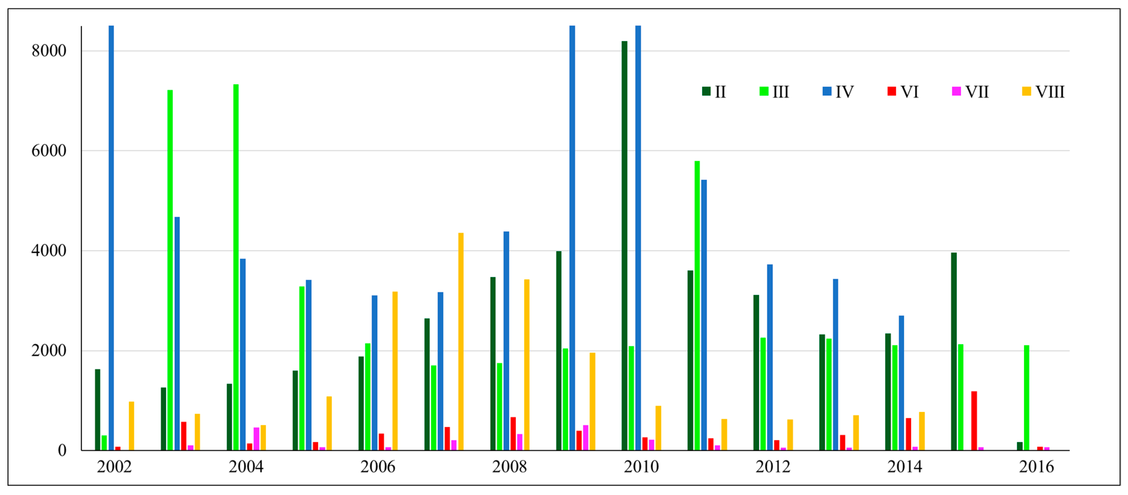
Figure 5.
The number of pixels in each individual year for the patterns II–IV (increasing trends) and VI–VIII (decreasing trends).
Figure 5.
The number of pixels in each individual year for the patterns II–IV (increasing trends) and VI–VIII (decreasing trends).

Figure 6.
The second transition years (a) and the duration of vegetation changes (b) in the logistic pattern which has two transition years during the observation period. The number of pixels in each individual year for the second transition years are shown in the histogram below a. The histogram below b is the proportions of four duration periods.

Figure 7.
Future status of vegetation changes in the Shiyang River Basin. The proportion of each status is shown in the item of the legend.
Figure 7.
Future status of vegetation changes in the Shiyang River Basin. The proportion of each status is shown in the item of the legend.

Figure 8.
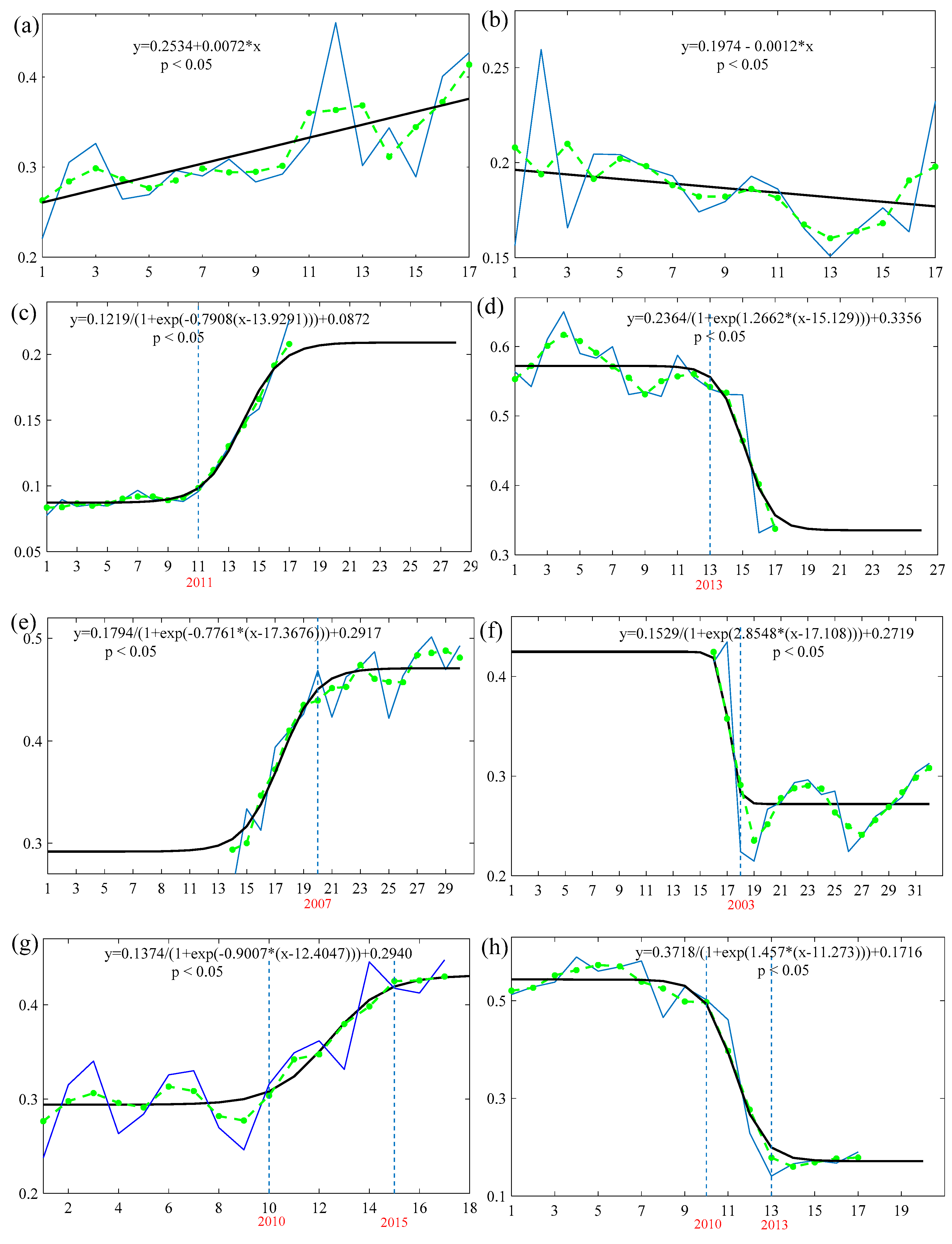
Processes of vegetation gradual changes in the eight reference sites (a–h) which are shown in Figure 3. The number of each subfigure corresponds to the number of reference sites in Figure 3, in which the pattern of each site detected by our framework is shown. The contents in each site include profiles of the original NDVI timeseries (blue solid line), the smoothed timeseries (green dotted line) and the fitting temporal profile (black line), the fitting function, and locations of the transition year (red word). Values in the horizontal axis in each subgraph represent the serial numbers in the prolonged timeseries (k) which ranges from 1 to L while that in the vertical axis are mean May to September NDVIs. The landscape transformation or modification for each site during the observation period are listed in Table 3.
Figure 8.
Processes of vegetation gradual changes in the eight reference sites (a–h) which are shown in Figure 3. The number of each subfigure corresponds to the number of reference sites in Figure 3, in which the pattern of each site detected by our framework is shown. The contents in each site include profiles of the original NDVI timeseries (blue solid line), the smoothed timeseries (green dotted line) and the fitting temporal profile (black line), the fitting function, and locations of the transition year (red word). Values in the horizontal axis in each subgraph represent the serial numbers in the prolonged timeseries (k) which ranges from 1 to L while that in the vertical axis are mean May to September NDVIs. The landscape transformation or modification for each site during the observation period are listed in Table 3.

Figure 9.
The temporal trajectories of the five regions selected for validation. The number of each subfigure corresponds to the number of the validated region in Figure 3 and Figure 4. The pattern and the transition years of each region detected by our framework are obtained from Figure 3 and Figure 4, respectively and are listed in the table on the low right of the figure. The values in the vertical axis of each subgraph are the mean NDVI of all the pixels which had the same transition years as that listed in the table on the low right corner.


Table 1.
Patterns of vegetation gradual changes are discussed in our study. Features of each pattern, including trend, transition years, duration and forecast of vegetation change are shown below. Options with the symbol ◊ will be excluded for discussion in our study, while the others will be considered for analyses in the study.
| Patterns | Trends (b Value in Equation (4) and Slope Value in Equation (6)) | Number of the Transition Years (num) | Duration of Vegetation Changes | Forecast | ||
|---|---|---|---|---|---|---|
| No-trend | IX | ◊ | ◊ | ◊ | ◊ | ◊ |
| Linear | I |  | Slope > 0 | 0 | ◊ | Keep increasing |
| V |  | Slope < 0 | 0 | ◊ | Keep decreasing | |
| Exponential | II |  | b > 0 | 1 | ◊ | Keep increasing |
| VI |  | b < 0 | 1 | ◊ | Keep decreasing | |
| Logarithmic | III |  | b > 0 | 1 | ◊ | High stable level |
| VII |  | b < 0 | 1 | ◊ | Low stable level | |
| Logistic | IV |  | b > 0 | 2 | √ | High stable level |
| VIII |  | b < 0 | 2 | √ | Low stable level | |
Table 2.
Coverage of vegetation (NDVImax ≥ 0.2) change patterns in the Shiyang River Basin based on our framework. Each pattern is divided into two types according to the positive or negative trend in NDVI timeseries.
Table 2.
Coverage of vegetation (NDVImax ≥ 0.2) change patterns in the Shiyang River Basin based on our framework. Each pattern is divided into two types according to the positive or negative trend in NDVI timeseries.
| Patterns of Significant Change in Vegetation | No-trend | |||||||||
|---|---|---|---|---|---|---|---|---|---|---|
| Linear | Linear | Exponential | Exponential | Logarithmic | Logarithmic | Logistic | Logistic | |||
| Type | (+) | (−) | (+) | (−) | (+) | (−) | (+) | (−) | ||
| Coverage (%) | 18.43 | 1.73 | 13.53 | 1.88 | 14.49 | 0.79 | 30.07 | 6.46 | 12.61 | 100 |
Table 3.
Landscape transformations or modifications in the eight reference sites for validation (Figure 8).
Table 3.
Landscape transformations or modifications in the eight reference sites for validation (Figure 8).
| Site | Land Cover (2001) | Land Cover (2017) | Change Time | The Known Facts | Evidence |
|---|---|---|---|---|---|
| a | Forest | Forest | The growth of trees | Report in newspaper [40] | |
| b | Grasslands | Bare lands | The surface reflectivity gradually brightened from dark | Landsat images on Google Earth Pro | |
| c | Desert lands | Forest | 2011 | Road greening | High resolution images on Google Earth Pro |
| d | Farmlands | Greenhouse | 2013 | Greenhouses kept increasing from 2013 to 2017 | High resolution images on Google Earth Pro |
| e | Desert lands | Farmlands | 2007 | The surface reflectivity gradually transformed from bright to dark | Landsat images on Google Earth Pro |
| f | Farmlands | Urban areas | 2003 | Urbanization | High resolution images on Google Earth Pro |
| g | Grasslands | Grasslands | 2010 | The implementation of the grassland protection projects | Report in newspaper [41] |
| h | Farmlands | Urban areas | 2010 | Urbanization | High resolution images on Google earth |
© 2019 by the authors. Licensee MDPI, Basel, Switzerland. This article is an open access article distributed under the terms and conditions of the Creative Commons Attribution (CC BY) license (http://creativecommons.org/licenses/by/4.0/).
Share and Cite
MDPI and ACS Style
Wang, J.; Xie, Y.; Wang, X.; Dong, J.; Bie, Q. Detecting Patterns of Vegetation Gradual Changes (2001–2017) in Shiyang River Basin, Based on a Novel Framework. Remote Sens. 2019, 11, 2475. https://doi.org/10.3390/rs11212475
AMA Style
Wang J, Xie Y, Wang X, Dong J, Bie Q. Detecting Patterns of Vegetation Gradual Changes (2001–2017) in Shiyang River Basin, Based on a Novel Framework. Remote Sensing. 2019; 11(21):2475. https://doi.org/10.3390/rs11212475
Chicago/Turabian StyleWang, Ju, Yaowen Xie, Xiaoyun Wang, Jingru Dong, and Qiang Bie. 2019. "Detecting Patterns of Vegetation Gradual Changes (2001–2017) in Shiyang River Basin, Based on a Novel Framework" Remote Sensing 11, no. 21: 2475. https://doi.org/10.3390/rs11212475
Note that from the first issue of 2016, this journal uses article numbers instead of page numbers. See further details here.