Article

Evaluation of Atmospheric Correction Algorithms over Spanish Inland Waters for Sentinel-2 Multi Spectral Imagery Data

1
Image Processing Laboratory, Laboratory of Earth Observation. Universitat de València, C/Catedrático José Beltrán, 2, 46980 València, Spain
2
Institut Cavanilles de Biodiversitat i Biología Evolutiva, Universitat de València, C/Catedrático José Beltrán, 2, 46980 València, Spain
*
Author to whom correspondence should be addressed.
Remote Sens. 2019, 11(12), 1469; https://doi.org/10.3390/rs11121469
Submission received: 23 April 2019 / Revised: 14 June 2019 / Accepted: 18 June 2019 / Published: 21 June 2019

Abstract

:
The atmospheric contribution constitutes about 90 percent of the signal measured by satellite sensors over oceanic and inland waters. Over open ocean waters, the atmospheric contribution is relatively easy to correct as it can be assumed that water-leaving radiance in the near-infrared (NIR) is equal to zero and it can be performed by applying a relatively simple dark-pixel-correction-based type of algorithm. Over inland and coastal waters, this assumption cannot be made since the water-leaving radiance in the NIR is greater than zero due to the presence of water components like sediments and dissolved organic particles. The aim of this study is to determine the most appropriate atmospheric correction processor to be applied on Sentinel-2 MultiSpectral Imagery over several types of inland waters. Retrievals obtained from different atmospheric correction processors (i.e., Atmospheric correction for OLI ‘lite’ (ACOLITE), Case 2 Regional Coast Colour (here called C2RCC), Case 2 Regional Coast Colour for Complex waters (here called C2RCCCX), Image correction for atmospheric effects (iCOR), Polynomial-based algorithm applied to MERIS (Polymer) and Sen2Cor or Sentinel 2 Correction) are compared against in situ reflectance measured in lakes and reservoirs in the Valencia region (Spain). Polymer and C2RCC are the processors that give back the best statistics, with coefficients of determination higher than 0.83 and mean average errors less than 0.01. An evaluation of the performance based on water types and single bands–classification based on ranges of in situ chlorophyll-a concentration and Secchi disk depth values- showed that performance of these set of processors is better for relatively complex waters. ACOLITE, iCOR and Sen2Cor had a better performance when applied to meso- and hyper-eutrophic waters, compare with oligotrophic. However, other considerations should also be taken into account, like the elevation of the lakes above sea level, their distance from the sea and their morphology.

Graphical Abstract

1. Introduction

The radiance over water measured by satellite sensors has two important contributors: (1) the water itself, due to the interaction of sunlight with the optically active constituents (OACs), namely pure water, phytoplankton, Colored Dissolved Organic Matter and (CDOM) and Non-algal Particulates (NAP) or suspended sediments; and (2) the atmosphere, made up of atmospheric gases and aerosols. The latter represents about 90% of the signal measured by the satellite sensor [1]. This high proportion indicates that the correction of the impact of the atmosphere on the signal captured by the satellite sensor is a fundamental step in the processing chain for obtaining accurate water quality variables. Therefore, low uncertainty surface reflectance products are essential for obtaining an adequate retrieval from remote sensing [2,3]. These retrievals have been produced regularly in recent decades with more or less accuracy in different regions of the planet and for several water types. Prieur and Sathyendranath [4] determined that it was possible to separate the water masses into two cases according to the correlation between the different OACs, the Case 1 waters (or oceanic waters) and Case 2 waters (or coastal and inland waters). Wang [5] has determined that for typical Case 1 waters, the water-leaving reflectance contributions at Top Of Atmosphere (TOA) to the signal measured by sensors varies for different bands of the visible spectrum, with the highest atmospheric contribution in the blue-green bands close to 12%. For Case 2 waters, several situations have been found and Wang [5] remarks that the percentage of water-leaving reflectance contributions at TOA differs depending on whether the waters are dominated by suspended sediments or CDOM. These OACs have a very distinct effect, with Total Suspended Matter (TSM) producing a reflectance increase in the green and red bands, while CDOM increases absorption (reducing reflectance) in the blue bands.
Obtaining an accurate estimation of the water-leaving reflectance and therefore good input for retrieving water quality concentrations, is then an important step. This atmospheric correction (AC) procedure subtracts the atmospheric contribution (aerosols scattering effects), sunglint and whitecaps from the TOA signal [6]. There is increasing interest in evaluating the performance of different atmospheric correction (AC) processors on inland and coastal waters for obvious reasons: they constitute our main sources of drinkable water, are widely used for recreation and contain high biodiversity (40% of the marine and freshwater biomass [7]). For the present analysis, we have selected six AC processors to be applied on Sentinel-2 data: Atmospheric correction for OLI ‘lite’ (ACOLITE), Case 2 Regional Coast Colour (here called C2RCC), Case 2 Regional Coast Colour for Complex waters (here called C2RCCCX), Image correction for atmospheric effects (iCOR), Polynomial-based algorithm applied to MERIS (Polymer) and Sentinel 2 Correction (Sen2Cor). All these processors are free for the users and are quite simple to implement and apply. Retrievals obtained by each processor are validated with in situ measurements.
The work developed here is part of the research done within the Ecological Status of AQuatic Systems with Sentinel satellites (ESAQS) project, funded by the Prometeo Programme (Generalitat Valenciana, Spain). The aim of ESAQS is to develop and validate algorithms for estimating ecological quality indicators of water bodies in the region of Valencia (south-eastern Spain); for example chlorophyll-a (Chl-a), Secchi disk depth ( Z s d ), Colored Dissolved Organic Matter (CDOM) and suspended solids [8,9]. In this context, several small-sized lakes and some reservoirs located in the SE of Spain have been selected and biophysical parameters and water-leaving reflectances have been analyzed using satellite imagery and in situ data from field campaigns. The lakes studied here can be classified into several water types based on their chlorophyll-a content and water transparency. In some cases, the water type in a lake changes visibly throughout the year due to the influence of the surrounding farming and industrial activities on the water content. The study area is the Jucar hydrographic basin. Geographically, it is located in the central-eastern part of the Iberian Peninsula. It is a transitional area located between a mountainous interior, the Iberian and Baetic systems and the coastal alluvial plain. In the alluvial platform lies the natural reserve of the Albufera of Valencia, one of most important freshwater lagoons with an area of approximately 21,120 hectares. The predominant climate in the area is typical semi-arid Mediterranean, with dry, warm summers and mild winters. The elevations of these lakes and reservoirs ranges from 0 (Albufera lagoon) to about 700 mamsl (Contreras reservoir) and their distance to the Mediterranean Sea ranges from 3 to more than 17 km (see details in Table 1). The geographical environment gives these inland waters particular shapes, so the determination of such morphometric parameters as the shoreline development index can help us describe the shape and physical characteristics of these lakes, lagoons and reservoirs [10]. Twenty-one cloudless Sentinel 2-MultiSpectral Imagery Level 1 scenes were free-downloaded from the Copernicus Open Access Hub of the European Space Agency (ESA) [11] to match-up with the ESAQS project field campaign days.
Similar types of exercise have been previously done before using S2-MSI data [12]; for example, in the Atmospheric Correction Inter-comparison eXercice (ACIX) [3]. ACIX is an international initiative by the Committee on Earth Observation Satellites (CEOS), the National and Aeronautic and Space Administration (NASA) and ESA, the aim of which is “to explore the different aspects of every AC processor and the quality of the surface reflectance products”. The performance of ACOLITE and SeaDAS at coastal sites has been evaluated by ACIX on the coast of Romania, Italy and Belgium. The Global Lakes Sentinel Services (GLASS), funded by the European Commission (EC), researched, applied and compared several commercial and open source AC algorithms over European inland waters (Finland, Netherlands, Estonia, Italy and Sweden) [13]. Other initiatives [14] have analyzed several AC processors like C2RCC, ACOLITE, Polymer and the “standard” Sentinel 2 Correction (Sen2Cor) in the Baltic Sea. In Latin America, Souza Martins et al. [15] applied and assessed the performance of the Second Simulation of a Satellite Signal in the Solar Spectrum (6SV), ACOLITE and Sen2Cor AC processors to S2-MSI over Amazon floodplain lakes.

2. Study Area, Data and Approaches
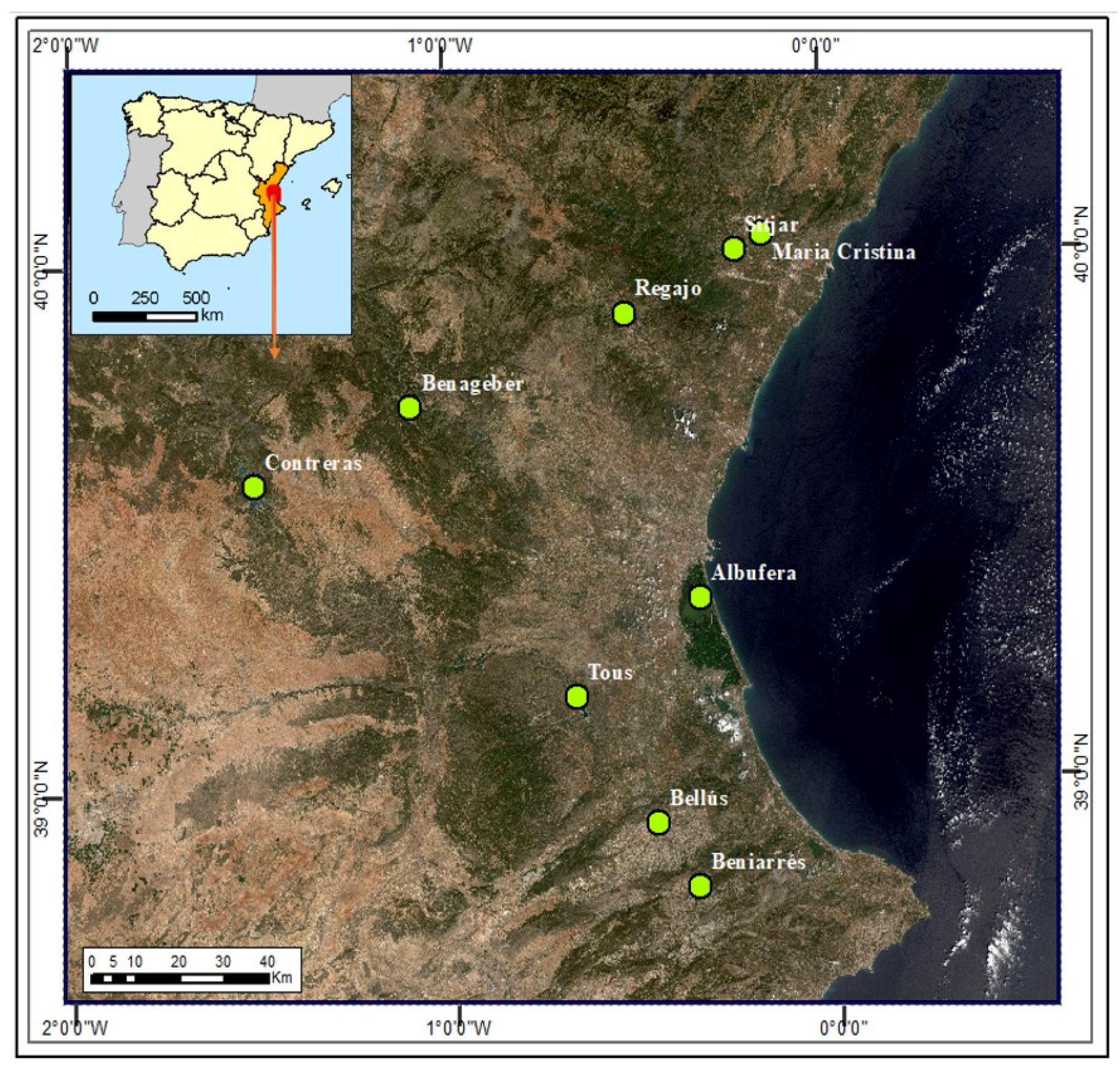
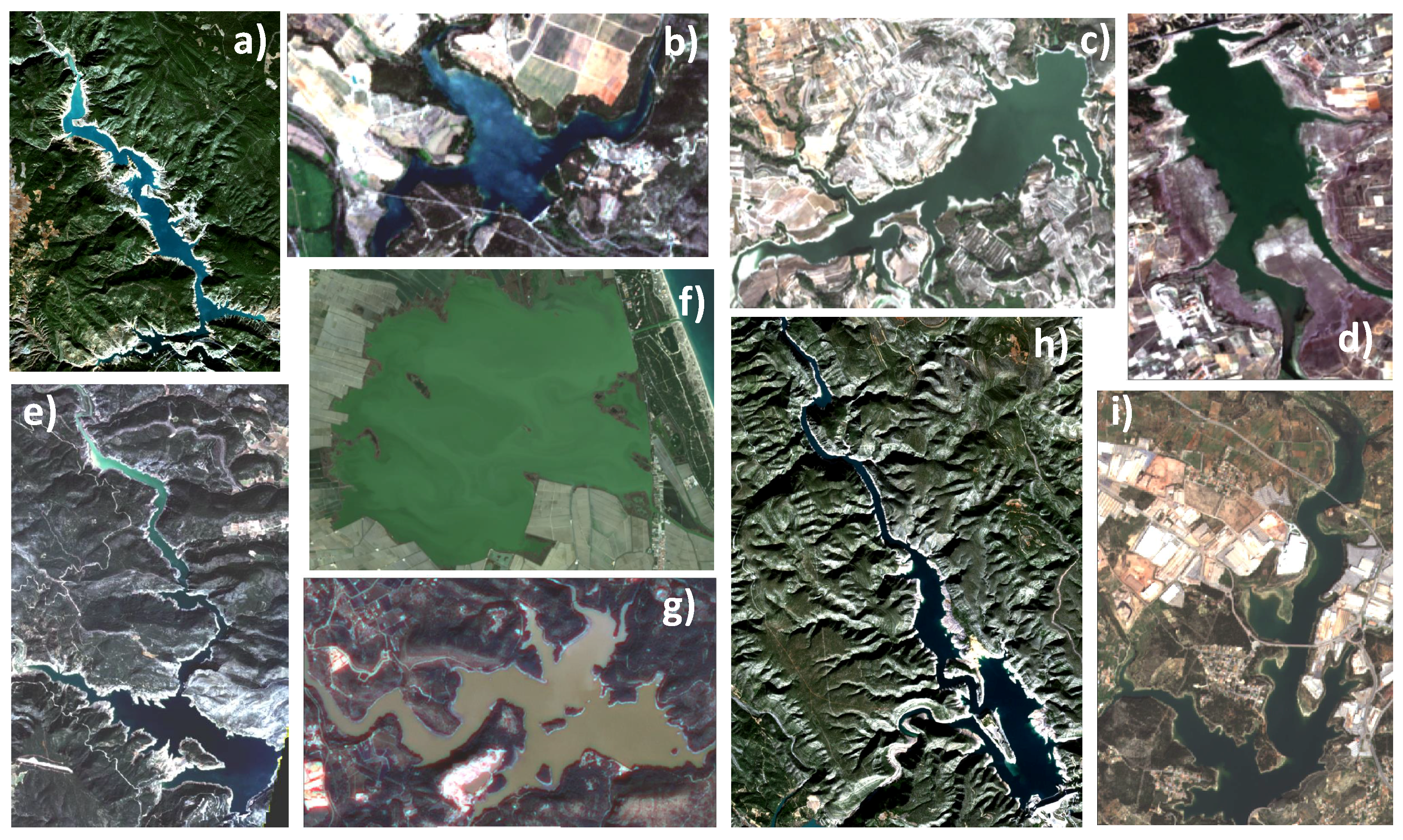
2.1. Study Area

Since the beginning of the ESAQS Project in December 2016, many field campaigns have been carried out in the Valencia region. These field campaigns were done on cloud-free days coinciding with Sentinel-2 satellite overpasses within a time window of ± 3 h. Eight reservoirs and one coastal lagoon have been monitored: Benagéber, Bellús, Beniarrés, Contreras, M a Cristina, Regajo, Sitjar, Tous and the lagoon of the Albufera of Valencia. Figure 1 shows their location on the Spanish Mediterranean coast. Figure 2 shows the irregular and diverse shapes of these small water masses and Table 1 provides details about the surface area—calculated with maximum water level height- and meters above mean sea level (mamsl), as well as the distance to the sea and the shoreline ratio [10]. This information can be useful to explain some of the behaviours of the AC algorithms on the different water masses. Most of the field campaigns were carried out in autumn, winter and spring and only four in summer due to more favourable weather conditions and availability of staff and equipment. Among others, two biophysical parameters measured in the field campaigns are the Chl-a and Z s d . These were measured by the Limnology Research Team of the University of Valencia [8]. Chl-a data were obtained from water samples by the spectrophotometric method. Samples were filtered through 0.4–0.6 μ m GF/F glass fiber filters, extracted according to standard methods by Shoaf and Lium [16] and the calculation methods of Jeffrey and Humphrey [17]. Z s d data was measured with a Secchi disk. It is divided into four quarters, each one painted black and white. The measurement procedure for obtaining the Z s d is to lower it slowly in the water until it disappears from sight. When that happens, it is possible to obtain the Z s d [9]. Table 2 describes the in situ minimum and maximum values of the Chl-a and Z s d parameters, together with other statistics.
The study area covers a wide gradient of trophic states, from ultraoligotrophic to hypertrophic. Following the trophic classification scheme for lake waters proposed by the Organisation for Economic Cooperation and Development [18], we applied this scheme to our reservoirs, lakes and lagoon based on value ranges of Chl-a and Z s d measured in situ. This classification is shown in Table 3. The total number of properly measured points is 53. For each reservoir one to five measuring points were taken at a suitable distance from shoreline to avoid mixed pixels (land-water mixed and bottom reflectance contamination). In the same set of lagoons, lakes and reservoirs, Pereira-Sandoval et al. [9] demonstrated that due to the variability presented in the Chl-a values, a better adjustment in the result of the algorithms was obtained if the algorithms were calibrated and applied according to the trophic level presented. For this reason and in order to simplify the analysis presented here, we have grouped the water types into three main classes (Table 3):
The aggregation into three water types is later used in several statistical analyses and plotting tests in order to understand how the atmospheric correction processors are affected by the different water components. Thus, of the 29 field campaigns carried out in lakes and reservoirs in the Valencia region, eight have data that belong to water Type 1, seven to water Type 2 and fourteen to water Type 3, see Table 4, last column.

2.2. Satellite Data

The Sentinel-2 satellites are part of the Copernicus Programme (European Commission and European Space Agency), which have on-board the MultiSpectral Instrument (from now on S2-MSI). Though S2-MSI was designed for land studies, it is possible to use it for water studies thanks to its optimized spatial resolution (10–20 m), good radiometric resolution, adequate band configuration and short revisit time (5 days using the Sentinel-2A and Sentinel-2B satellites at the equator and 2–3 days at mid latitudes), making it an optimal instrument for remotely monitoring lakes and reservoirs with a reduced surface area, as well as coastal waters. MultiSpectral Instrument (MSI) imagery Level1 (L1) from Sentinel-2A and Sentinel-2B are processed and evaluated. In this work, 21 cloudless S2-MSI L1 scenes were free-downloaded from the Copernicus Open Access Hub of the European Space Agency [11] in match-up with the ESAQS project field campaign days (see details in Table 4). The images were resampled to 10 m as part of the preprocessing. The difference between the campaign days (29) and the final number of S2-MSI L1 processed is due either to problems derived from the imagery (e.g., containing haze or cirrus clouds not observed from the ground) or to equipment issues (spectroradiometer malfunctioning).

2.3. Above-Water Radiometry Measured In Situ

All measured stations selected in the different lagoons and lakes were made at a distance of at least 3 pixels (30 m) from the shoreline to avoid or at least reduce the effect of mixed pixels, bottom reflectance and adjacency contamination from the surrounding land and breaking surf near shorelines [19]. The water-leaving radiance ( L w ) was obtained from measurements taken from the bow of a boat by sequentially measuring the total observed radiance ( L t ), which includes the contributions of diffuse sunlight reflected by the water surface ( L g ) and the sky radiance ( L s k y ) used for the calculation of L g . For the field measurements, we used a ASD FieldSpec® HandHeld 2 spectroradiometer, which has a wavelength range of 325 to 1075 nm and a spectral resolution of 1 nm and an Ocean Optics (HR 4000) spectrometer ranging from 200 to 1100 nm at a spectral resolution of 0.2 nm. In accordance with recommendations by experts and the existing protocols in the bibliography [20,21,22], the measurements were carried out with a zenith angle of 40 and an azimuth angle of 135 to minimize sunglint perturbations. The radiometer’s field of view (FOV) was delimited using a FOV of 8 . Once these general issues were defined, between three to five points were measured for each reservoir and lake. The number differs depending on the shape of the water mass and its surface area (see Figure 2 and Table 4). For each point, the measurement procedure followed consisted of taking five measurements of the water-leaving radiance ( L w ) and total downward irradiance E d using a reflectance plaque made of Spectralon® ( L r e f ). This plaque is used to normalize the uncalibrated radiance measurements from E d . We used a gray reflectance plaque (25% nominal reflectance) that is required for the minimization of changes of illumination conditions during measurements. With these data, the in situ remote sensing reflectance ( R r s ) is calculated from the following equations:
R r s = L w / E d
L w = L t L g
L g = r h o L s k y
R r s = ( L t L g ) / E d
to obtain the L w , it is necessary to remove the radiance measured from the sky L g from the observed radiance L t . The result of that difference is divided by the total downward irradiance E d .
Rho is the surface reflectance used to correct the radiance of the sky. In accordance with wind speed data measured in the ESAQS field campaigns (values equal to or less than 5 m per second) and consistent with the reflectance factor provided by Mobley 1999 and Mobley 2015 [20,23], we have decided to use a constant rho factor value equal to 0.028.
E d = ( L r e f / R r e f ) / p i
the E d term is obtained through the division between L r e f (the reference radiance measured using the reflectance plaque) and R r e f of the plaque, provided by the vendor. Up to this point, we have worked with radiance units; therefore, it is necessary to cancel out the units dividing the terms L w and E d by the value of pi to obtain the units of steradian. Finally to obtain the spectral remote sensing reflectance, we have applied the following equation:
R = ( R r s p i )
where to obtain R r s , it is necessary to multiply the terms previously obtained by the value of pi. Once the in situ remote sensing reflectance spectra is obtained, it is convoluted to the S2-MSI spectral bands using the Sentinel-2 Spectral Response Functions S2-SRF (SRF v2.0) [24].

2.4. Atmospheric Correction Approaches

The requirements for the selection of the atmospheric correction algorithms are based on their availability and cost zero, the ease for understanding their implementation and the possibility of correcting inherent effects like sunglint and adjacency of land pixels. All these processors are able to correct for the effect of the aerosol contributions and remove them from the water-leaving radiance with different levels of accuracy.
ACOLITE is an atmospheric correction processor for coastal and inland waters developed by the Management Unit of the Mathematical Model of the North Sea (MUMM) in Belgium [25]. It performs atmospheric correction using the dark spectrum fitting approach by default but it can be configured to use the exponential extrapolation [26,27,28,29] approach. In this work, we have applied the ACOLITE v.beta. 20180925 processor using the default approach in order to check its performance for the different water types. According to Reference [30], the algorithm would work over clear and mixed clear/turbid waters for most sensors but it would require the presence of SWIR bands to work over scenes with only turbid waters.
Case 2 Regional Coast Colour (C2RCC) is a development of the original Case 2 Regional processor [31,32]. It relies on a database of radiative transfer simulations of water-leaving reflectance (water signal) and related Top-Of-Atmosphere (TOA) radiances (satellite signal). The inversion of water signal and satellite signal is performed by neural networks. A characterization of optically complex waters through its inherent optical properties (IOPs) is used along with the coastal atmospheres to parameterize radiative transfer models for the atmosphere over the water body. The C2RCC has been improved to cover extreme ranges of scattering and absorption, now using a 5-component bio-optical model. The in-water modelling uses a Hydrolight model and the atmospheric radiative transfer is based on the SOS model [33] with aerosol properties derived from AERONET measurements. C2RCC has two versions: a version called the normal net (here C2RCC), with typical ranges of IOPS; and an extreme net version (here C2RCCCX), for extreme ranges of absorption and scattering. It is available on the SeNtinel Application Platform (SNAP v.6.0) [34]. The images were processed here according to the default processing parameters.
iCOR, previously known as OPERA [35,36], is a generic scene and sensor atmospheric correction algorithm for land and water targets. The following steps are performed: (i) identification of land and water pixels; (ii) land pixels are used to derive Aerosol Optical Thickness (AOT) based on an adapted version of the method developed in Reference [37] in the SCAPE-M algorithm; (iii) an adjacency correction is performed using SIMEC [36] over water and fixed background ranges over land targets; and (iv) the radiative transfer equation is solved. iCOR uses MODTRAN 5 [38] Look Up Tables (LUT) to perform the atmospheric correction and needs information about the solar and viewing angles (Sun Zenith Angle (SZA), View Zenith Angle (VZA) and Relative Azimuth Angle (RAA)) and a digital elevation model (DEM). The images were processed here according to the default processing parameters, applying the SIMEC adjacency correction. The present version of iCOR (v.1.0.0) does not correct for sunglint effects.
Polymer (Polynomial based algorithm applied to MERIS [39]) is an atmospheric correction algorithm for processing oceanic waters with and without the presence of sunglint. Polymer is a physical model based on a spectral optimization method called spectral matching. It applies all the spectral bands to make the atmospheric and sunglint correction; therefore, AC is not exclusively based on the NIR signal. The images were processed here according to default processing parameters in Polymer v.4.6. Polymer is used by the Ocean Colour- Climate Change Initiative [40]. This processor contains quality flags but they differ from C2RCC (Table 5).
Sentinel 2 Correction (Sen2Cor) is designed exclusively for Sentinel-2 Level 2A land products [41]. It is based on the dark dense vegetation approach (DDV) [42]. This method assumes that the vegetation is sufficiently dark and the ratio between the bottom of the atmosphere reflectance at different wavelengths is constant. This algorithm requires some pixels in the image to correspond to dense dark vegetation. Once the presence of such pixels is established, the algorithm automatically chooses these pixels, derives the AOT and corrects the image [43]. One main difference with the preceding processors is that it considers a lambertian surface, while the air water interface has a specular reflection [44]. The images were processed using the default mode.

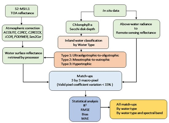
3. Preparation of Match-Ups

Once the S2-MSI data atmospherically corrected by processors were obtained, we extracted the pixel value reflectance on a 3-by-3 window centered on the geographical coordinates of the in situ stations. To assess the performance between the imagery reflectance and the in situ reflectance, we did two tests: (i) using all match-ups without applying quality control flags; (ii) applying quality control flags. The selection criteria for match-ups included a time window of ± 3 h between the satellite overpass and the in situ measurement times. The image pixels are extracted over a 3-by-3 S2-MSI macro-pixel (30-by-30 m) centered on in situ measurements for ACOLITE, C2RCC, C2RCCCX, iCOR, Sen2Cor and Polymer processed scenes. We calculated the average reflectance for each macro-pixel, applying a regular outlier calculation to remove suspicious pixels from the average. We recalculated the mean and standard deviation with the valid pixels remaining and those were used to determine the coefficient of variation, which has to be below 15% to assure homogeneity. Finally, the number of remaining pixels within the macro-pixel are counted and if the number is higher than half the original macro-pixel (i.e., 5 pixels over 9), the macro-pixel is valid and taken into account [45,46]. The total number of macro-pixels (N) left by type of processing is shown in Table 6, middle column.
The description of the flags used to mask out invalid pixels when applying quality control flags included in C2RCC, C2RCCCX and Polymer- is specified in Table 5. With the unmasked pixels left, the outlier calculation is carried out as explained in the previous paragraph. The total number of macro-pixels left by processor is shown in the right-hand column of Table 6. The average number of match-ups is around 50 points, C2RCCCX has the minimum number of match-ups (37), while Sen2Cor has the maximum with 62 points (See Figure 3).
We have evaluated the performance of the S2-MSI reflectances when compared to the in situ reflectances and plotted the results and statistics per AC processor. We used ordinary least square metrics: the coefficient of determination ( R 2 ) and the root mean square error (RMSE). We also derived other metrics to evaluate non-Gaussian distributions in order to understand the systematic error and accuracy through the bias and the mean absolute error (MAE) [47].

4. Results

It does not seem feasible to develop a universal algorithm for deriving bio-optical parameters in variable and complex waters. For that reason, a previous classification of the water types is a good compromise for improving the inversion of bio-optical parameters [48]. According to the results obtained by Pereira- Sandoval et al. [9], we decided to apply a water type classification, grouping the reservoir data into three types based on the Chl-a and Z s d values: ultraoligotrophic-to-oligotrophic (Type 1), mesotrophic-to-eutrophic (Type 2) and hypertrophic (Type 3) defined in Section 2.1. This pre-classification would help us understand the results of the performance of each AC processor when taking into account the water type.

4.1. Results with All the Match-Ups

Figure 3 shows the scatter plots with the spectral performance by each AC processor. The relationship between the reflectance measured in situ (IS) is plotted against the reflectance derived by the MSI sensor (OBS). Each S2-MSI band is depicted by a specific color. The water type is symbolized by a circle for Type 1, a cross for Type 2 and a square for Type 3.
In general, it is possible to distinguish two major groups: in the first group, C2RCC, C2RCCCX and Polymer show quite a good performance, with small dispersion and measurements aligned to the 1:1 lines, though with clear biases; and in a second group, ACOLITE, iCOR and Sen2Cor depict less favourable results. C2RCC, C2RCCCX and Polymer show low mean average errors (MAE) from 0.0089 (Polymer) to 0.01 (C2RCC) and coefficients of determination ( R 2 ) ranging from 0.81 (C2RCCCX) and up to 0.83 (Polymer), when plotting all bands together. The plots also show a satisfactory adjustment to the 1:1 line, especially for C2RCCCX and Polymer in Types 2 and 3 waters (mesotrophic and hypertrophic waters). However, C2RCCCX seems more restrictive in the procedure with a lower number of match ups (37) compared to C2RCC (53) and Polymer (52). Two common patterns are shown in these AC processors: C2RCC, C2RCCCX and Polymer show an overestimation of some data in the visible bands (443, 490 and 560 nm), especially for Type 1 waters (ultraoligotrophic-to-oligotrophic) while the bulk of the data is below the 1:1 line. In the plots with the ACOLITE, iCOR and Sen2Cor processing, results are not so good, with a lower accuracy range (MAE) between 0.022 for ACOLITE to 0.038 for iCOR and R 2 values from 0.02 for iCOR, to 0.34 for Sen2cor. One remarkable issue is that the accuracy seems higher or lower depending on the water type. For these three processors, it is possible to identify two behaviours in the dataset: a cloud of points with high dispersion above 1:1 line for in situ reflectance below 0.04 values; and a second cloud mainly pertaining to water of Type 3 (squared symbol), apparently with a better fit to the 1:1 line for practically all bands.
In order to assess the spectral dependency errors for all processors, Figure 4 shows the statistical analysis applied to all spectrum bands by AC processor: R 2 , MAE, bias and the absolute RMSE per band are shown. Some patterns can be identified: C2RCC, C2RCCCX and Polymer–the green, red and yellow lines respectively- present the highest R 2 values across all bands. Visible bands show the best result for Polymer and C2RCC. Both processors have similar values but Polymer has a lower MAE range between 0.009 to 0.0014 (Figure 4, top right) with R 2 from 0.29 to 0.91 (Figure 4, top left). C2RCC presents a MAE range between 0.007 to 0.020 and R 2 values from 0.48 to 0.94. In red-NIR bands, Polymer presents a MAE range from 0.002 to 0.009 with a R 2 over 0.84. C2RCC shows a MAE between 0.02 to 0.013 and R 2 over 0.76, confirming the good performance of both processors.
The bias values of C2RCC, C2RCCCX and Polymer show negative values for the entire spectrum range, indicating a slight overestimation of the reflectance obtained by these three AC processors (Figure 4, bottom left). Sen2Cor and ACOLITE show a low positive bias, while iCOR increases the bias in the red and NIR bands quite impressively. Finally, the RMSE shows range values from 0 to above 0.1, reaching 0.22 (Figure 4, bottom right). For ACOLITE, iCOR and Sen2Cor–dark blue, magenta and light blue lines respectively- the statistical results are notably less satisfactory compared to the previous group of processors. The R 2 values in the blue-green bands are very low, between 0.18 to 0.45. The NIR bands show the worst performance, with values close to 0 for wavelengths longer than 740 nm. The MAE range is slightly higher than for the previous group of AC, between 0.02 to 0.025, indicating less accuracy. ACOLITE and Sen2Cor have very regular MAE values (0 to 0.02) for all bands. A similar trend is shown in the RMSE line, with ACOLITE and Sen2Cor presenting a similar trend close to 0.03 for all bands. iCOR is the AC processor that shows the worst performance in this analysis.

4.2. Results with All the Match-Ups by Water Type

Figure 5 shows the results of the performance of the AC processors by water type. The first three lines of plots show the C2RCC, C2RCCCX and Polymer performance. In accordance with the general results shown in Figure 3, Polymer and C2RCC validate their good results. For water Type 1 (ultra-to-oligotrophic), Polymer maintains good results, with a MAE of 0.007 and R 2 value equal to 0.81, with the best performance. For water Type 2 (mesotrophic-to eutrophic), C2RCC and Polymer show similar performance, though Polymer has less absolute error (MAE 0.004) than C2RCC (0.007). The coefficient of determination is quite high for both processors, achieving values of 0.93. For water Type 3 (hypertrophic), Polymer again shows a quite good adjustment, but MAE increases to 0.015, closer to the one obtained in the general results of 0.008 (Figure 3). C2RCCCX seems to perform better for water types 2 and 3. The second group of processors does not perform as well, as already indicated. ACOLITE, Sen2Cor and iCOR in general show lower accuracy, but again, at least ACOLITE and Sen2Cor show some improvement in water types 2 and 3 ( R 2 values between 0.40 and 0.55 and MAE ranges from 0.012 to 0.022). For oligotrophic waters, the results are quite poor for all these processors. iCOR still shows the worst performance in water Type 2 with a big dispersion of data, practically no correlation and higher errors.

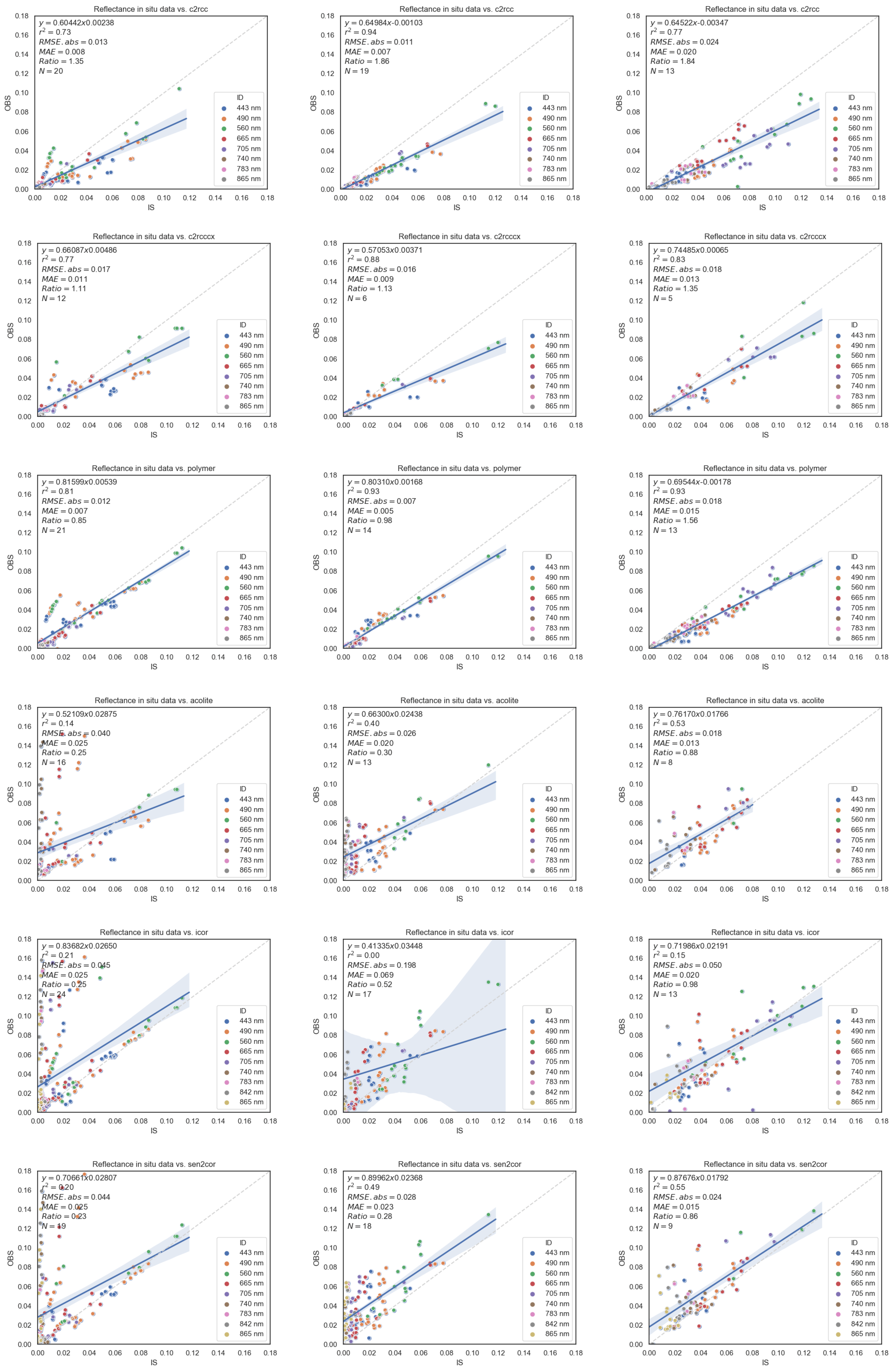
4.3. Results with All the Match-Ups by Water Type and Spectral Band

In order to better understand the results, Table 7 gives further details by separating each water type per AC processor and S2-MSI spectral band. For water Type 1, from 443 to 665 nm bands, Polymer has a lower MAE (0.004 to 0.015) and a higher R 2 range (0.55 to 0.89) than C2RCC, with MAE range of 0.006 to 0.020 and R 2 range 0.39 to 0.83. The highest MAE values correspond to the 490 nm band with values of 0.015 and 0.020, respectively for Polymer and C2RCC. In NIR bands, both processors give similar results, with slight better performing of C2RCC. Nevertheless, the errors are smaller than in visible bands. The R 2 range for Polymer are between 0.64 to 0.82 and for C2RCC are between 0.72 to 0.86, except for band 856 nm. This band has the lowest coefficient of determination, 0.006 and 0.12, correspondingly. In water Type 2, the visible spectral region shows optimum results in Polymer. Here, MAE is between 0.005 to 0.008 and the R 2 values range from 0.61 to 0.99. It is followed by C2RCC but with larger errors than Polymer (MAE between 0.011 to 0.018) and R 2 range between 0.72 to 0.98. In NIR spectrum, C2RCC and Polymer have similar results: MAE values between 0.001 to 0.006 and R 2 values between 0.92 to 0.99. In this water type the 865 nm band, in both AC processors, has a better performance than in water Type 1. Finally, for water Type 3, Polymer shows better results than C2RCC in the visible spectrum with a MAE range between 0.007 to 0.018 and R 2 range from 0.88 to 0.90. In NIR bands, Polymer has the better performance of the two processors, with MAE between 0.07 to 0.019. Band 865 nm performance is quite better here compared with C2RCC and C2RCCCX.
The ACOLITE and Sen2Cor improvements in water Type 2 (mesotrophic-to eutrophic) and Type 3 (hypertrophic) as mentioned in Section 4.2, are concentrated in the visible bands. ACOLITE has lower errors than Sen2Cor does, with MAE between 0.009 to 0.016 and a R 2 from 0.21 to 0.87. Sen2Cor errors range between 0.015 to 0.0024 and the R 2 between 0.10 to 0.80. iCOR numbers are very low for R 2 in all the bands and the three water types, however some slight improvements can be seen in the most complex waters (Type 3), with MAE between 0.011 to 0.019 and R 2 from 0.24 to 0.46 in the visible bands.

4.4. Results Applying Quality Flags

As mentioned, only C2RCC (both nets) and Polymer processors have quality flags that can be used to identify possible invalid reflectance (see Table 5 for the flags tested here). If these flags are applied, the number of match-ups is considerably reduced for C2RCCCX (27), but Polymer and the normal net of C2RCC keep a similar number of points (around 40). For all cases, the retrieval slightly underestimates the observations, but in general a good performance is observed, with R 2 values from 0.78 (C2RCCCX) up to 0.83 (Polymer), accuracy range (MAE) between 0.0074 to 0.01 and quite good adjustment to the 1:1 line (scatter plots not shown here). Polymer shows a better performance than C2RCC in the visible spectrum. For C2RCCCX, the restricted control of the quality flags provides fewer available match-ups, but results look similar to the normal net results, improving the statistics from the green to the NIR, lowering accuracy in the blue bands. Because the application of the quality flags changes the number of match-ups but did not noticeably affect the statistics, we finally decided to work with the whole dataset, which allowed us to compare results with the other three processors that do not raise flags.

5. Discussion

The radiance reaching the satellite sensor experiences multiple interactions within the atmosphere and the aquatic systems. Around seventy to ninety percent of a sensor-measured signal over the ocean and water bodies comes from the atmosphere. This high amount of “noise” has to be removed to obtain the water-leaving reflectance, the real value coming from the surface. To the inherent complexity of Case 2 waters, other external factors such as sunglint, wind speed, geometry of the observations and angles of the sun, together with possible land adjacency effects, are added to the sum of the sunlight detected by the sensor. This fact has led to the emergence of several AC processors that focus on oceanic, coastal and inland waters [5]. This is the reason reflectance derived from different AC processors must be analyzed and validated. These validation exercises are usually done over coastal waters and only in a few cases it is done over inland waters in the recent literature [3,12,13,14,15,19].
Atmospherically corrected S2-MSI data with six different AC processors are matched-up here to in situ measured reflectance in order to test, analyze and validate their performance. ACOLITE, C2RCC, C2RCCCX, iCOR, Polymer and Sen2Cor were tested over a set of reservoirs and lakes in the Eastern Iberian Peninsula. We deemed it necessary to apply a previous water type classification based on the trophic status of the lakes, according to the Chl-a and Z s d values measured in situ: Type 1 ultra-to-oligotrophic, Type 2 mesotrophic-to-eutrophic and Type 3 hypertrophic [18]. This water type classification would help to understand the performance of the different AC processor, because this factor can affect the results in several ways: for instance, the AC algorithm may have not been trained for a certain range or another IOPs, or it might influence on the magnitude of the adjacency effect (AE) in the visible bands [49].
General statistics have shown solid results for Polymer and C2RCC. As Warren et al. [12] pointed out, this good performance from the two algorithms, which use quite different approaches (see Section 2.4), means that Polymer and C2RCC reproduced the spectral shape of the in situ data better than the others. The accuracy of these results improved markedly after the application of the classification per water type, particularly for water Types 2 and 3 (increasingly complex waters). A more detailed analysis by bands (see Table 7) allowed us to identify the strengths and weaknesses of each AC processor according to the spectral region. A detailed discussion of the results per AC method follows.

5.1. Polymer, C2RCC and C2RCCCX

In the work of Steinmetz et al. [50], the Polymer algorithm (version 4.1) retrievals compared with MERIS simulated reflectance, showed results in Case 1 water of R 2 = 0.98 at 443 nm and R 2 = 0.93 at 560 nm. Steinmetz et al. validated Polymer using in situ data from the Satellite Intercomparison for Marine Biology and Aerosol Determination (SIMBADA) and with the MEris MAtchup In-situ Database (MERMAID), obtaining R 2 values equal to 0.78 for 443 nm, 0.62 for 490 nm and 0.89 for 560 nm. Those results are in the same range of values as the ones observed here most notably in Type 2 (see Table 7). Figure 3 shows a particular cloud of points in bands 443 nm, 490 nm and 560 nm, which is remarkably far from the rest. This cloud belongs to the points measured in the Contreras reservoir (Type 1) on 21 September 2018. This reservoir is located at an altitude of 700 mamsl and it is possible that this elevation could influence the atmospheric correction calculations due to the pressure change and the different distance to the sensor. Regrettably, in neither Reference [50] nor in the ATDB v1. Polymer Atmospheric Correction Algorithm [51] is there any mention about altitude induced issues. In Contreras, negative values were accounted for in the retrievals of band 865 nm. This led us to do a more exhaustive analysis in this reservoir and allowed us to identify the same situation on 30 November 2017 and on 13 June 2018 in bands 740 nm and 783 nm. Another important factor is related to wind speed. In Steinmetz et al. [50] and Reference [51], the authors point out an observation about the initial correction: “the wind speed at each pixel is not known accurately, therefore, a mis-estimation of the wind speed will lead to a mis-estimation of reflectances and can possibly lead to negative values of reflectances”. An over-correction of the atmospheric model, subtracting too much from the total signal, can produce these negative values. Ruescas et al. [52] applied Polymer to the Lake Mayor of the Lake Titicaca (Peru and Bolivia) (Chl-a near to 6 mg/m 3 ) at an altitude of almost 4 km and negative values were also obtained from band 665 nm. But in general Polymer shows a good performance. Qin et al. [14] evaluated Polymer in the Baltic Sea using MERIS. The authors obtained R 2 values between 0.6 to 0.81 in the visible bands. For NIR, the present results are better in water Types 2 and 3 of our lakes (see Table 7), with higher coefficients of determination and lower errors than those obtained in the Baltic Sea.
C2RCC generally shows a good performance, ranking second behind Polymer, with slight differences per water type and bands. In water Type 1, the cloud of points previously described in Polymer is visible here too (Figure 3). The coefficient of determination and the errors are worse than Polymer for bands 443 to 560 nm (Table 7). This behaviour of high MAE reappears in the other two water types, which indicates poor performance of the algorithm in the blue bands. This might be due to insufficient correction of a strong Rayleigh scattering by atmospheric gases below 500 nm. These results in Type 1 are in line with the validation made by the Case 2 eXtreme project [53]. The accuracy seems to improve in the green and red bands, but there is another decrease in the 865 nm band, coincident with the results in the rest of the AC algorithms applied. For water Types 2 and 3 the errors are a bit higher than for Polymer, as we summarized in Section 4.3. The C2RCC algorithm is under constant evolution and we are aware that there is a new version being testing that improves the accuracy for the blue bands and corrects for the sunglint effect (Roland Doerffer’s personal communication). We are looking forward to testing this new version in our waters.

5.2. ACOLITE, Sen2Cor and iCOR

We would like to emphasize the Sen2Cor and the ACOLITE results obtained in water Type 2 and Type 3. In the visible bands, their performance is relatively good after excluding band 443 nm. The ACOLITE range of errors are in accordance with those obtained by Souza et al. [15] using S2-MSI data in what they called “bright and dark lakes”. The differences in the error values could be due to the version of ACOLITE that they use. The ACOLITE processor using the dark spectrum fitting has been validated by Vanhellemont and Ruddick over Pléiades images in turbid coastal waters of Zeebrugge (Brussels) with good results [30]. Furthermore, the authors validated its good performance in the Thames Estuary [29]. Pereira-Sandoval et al. [9] applied the dark spectrum fitting approach on a specific water Type 3 (Albufera of Valencia) and had a suitable correlation coefficient and a low MAE. In the correction procedure, for each band, the darkest spectrum is fitted to different aerosol models in accordance with Moses [54]. It is known that variations in the altitude of inland waters from the mean sea level might introduce uncertainties in the estimation of aerosol content within the atmospheric column. In our study area, the lakes and reservoirs are at different altitudes, from 0 mamsl at the Albufera lagoon to more than 700 mamsl at the reservoir of Contreras. Therefore, one possible explanation of the moderately bad results obtained with ACOLITE and other processors in some cases, could be related to the altitude variable, since it might be affecting the estimation of the aerosol optical depth. Vanhellemont [29] has also warned about how processing a whole scene with the same aerosol model to estimate the path reflectance is likely insufficient. This idea is also supported by Pahlevan et al. and others [55,56] who said that if the aerosol properties are not well represented in the aerosol models over inland waters, high uncertainties are to be expected. The new version of ACOLITE updates the Look-up table (LUT) to be applied in dark spectral fitting, with default continental and maritime aerosol models, but with the possibility of supporting the addition of more aerosol models if required [29]. This means that the altitude of the different lakes within one scene, together with their location and distance to the coast, should be taken into account. Vanhellemont [30] stressed that to use the sample of a dark pixel over land would significantly benefit the atmospheric correction. However, ACOLITE does not apply an adjacency correction approach, in which, considering the necessity of having dark pixels from shadowy land, land pixels could contribute to the contamination of the reflectance of neighbouring water pixels. This is in fact a problem that can be extrapolated to other processors. At wavelengths above 700 nm, the impact of adjacency effects is particularly strong since neighbouring land pixels show distinctly higher reflectance [36]. Sterckx et al. illustrated that adjacency effects occur even for pixels several hundred metres away from the shoreline. Santer and Schmechting [57] indicated that for similar solar elevation, adjacency effects become negligible (less than 0.1%) only for a distance greater than 5 km from the shoreline. Thus, a correction of adjacency effects appropriate for the water/land environment is essential for reliable spectra when using approaches based in some degree on the darkest pixel correction. Both ACOLITE and Sen2Cor had in 740 and 783 nm higher values than the in situ measurements. Once established this fact, the adjacency correction may not be so necessary in some cases, that is, the perturbations caused by the adjacency effect show a great dependence on the position of the sun with respect to land, with the Fresnel value increasing if the sun is over the land portion of the image, which is not the case in many of the scenes of our study area [49].
Sen2Cor has non-negligible results in the visible spectra for water Type 2, excluding band 443 nm. Errors are generally higher, between 0.015 to 0.026, than results obtained by other authors using this AC processor [15]. This poor performance could be attributed to the algorithm approach, with the use of the DDV method, which is clearly better adapted to the atmospheric correction of land scenes. The best results obtained by Souza could be explained by the high presence of Amazon forest (darker vegetation) around the floodplain lakes. Other issues should be taken into consideration. As Bulgarelli and Zibordi [49] pointed out, the different geometry of the sensor observations, sun angles and water and land use type influence the adjacency effect contributions. Ruescas et al. [52] evaluated Sen2Cor over the Albufera lagoon, an extremely eutrophic lake with reflectance values that could approximate those of land and they had good response from the processor. According to the algorithm approach, the conclusion made was that the good response might actually be due to the high chlorophyll-a concentration (>50 mg/m 3 ) all year round in that water mass, which can reduce the adjacency effect, especially when the crops surrounding it are green during the spring and summer seasons [49].
In comparison with the previous processors, iCOR results were very poor. We had only moderate values in water Type 3 between bands 449 nm and 705 nm. iCOR is the only processor that uses an adjacency correction prior to the atmospheric correction. Bad results over water Type 1 and Type 2 could be explained by this factor. In the work of De Keukelaere et al. [58], observations are made over different lakes of Europe. They reported promising results for S2-MSI, except for band 443 nm, with and without adjacency correction, especially for Lake Marken. In the NIR, results are less promising, but with the SIMilarity Environment Correction (SIMEC) on, the adjacency correction seems to have a positive effect. De Keukelaere et al. [58] pointed out several important issues with iCOR. First, the surface reflectance should be representable by a linear combination of two pure green and a bare soil endmembers and the ocean and inland water do not meet this requirement unless there is some land within the scene. They recommended the user set an atmospheric optical thickness (AOT) value appropriate for each area when this requirement is not met. A second matter is that iCOR sets a fixed rural aerosol model as default. In an upcoming phase of iCOR, a valid water based AOT retrieval in combination with the current land based implementation will be done. So it is expected that this will reduce errors caused by extrapolation of AOT over large water bodies. Another issue related to the adjacency effect is that SIMEC should be used with caution “in high turbid waters, in waters with macrophyte growth or specific algae blooms or in areas where bottom effects are significant in the NIR (optically shallow waters)”. Several of those cases could be present on our study area, so a new water type classification taking these variables into account, could be a path to follow in future research activities.

5.3. Other Considerations

Sunglint is the reflection of sunlight off the water surface at the same angle a sensor is viewing this surface. The smoother the water surface, the higher the visibility of this silvery effect. But often water surfaces are in motion due to waves and currents, so the sunlight gets scattered in many directions, blurring the areas and causing the component of the radiance received by the sensor to be higher than the water-leaving radiance from sub-surface features. Since Sentinel-2 operates at near-nadir viewing angles, the probability of sunglint polluted radiance increases [59]. Of the six atmospheric correction processors tested here, Polymer includes detection and correction of sunglint. Future versions of C2RCC will also include this feature, but it is still under development. In any case, since our study areas are located in southeastern Spain and satellite overpasses in this area are usually around 10:50 local time (relative orbits 51 and 94 in descending mode), the sunglint contamination, if any, is visible in the right part of the scenes, not in the left where the lakes lie in most of the scenes. Only the Benageber and Contreras reservoirs, when using scenes on the 94 relative orbit, could be affected by sunglint. And these two cases are probably the most easily affected by other issues like adjacency effects and altitude related problems due to their high elevation and shapes (see Figure 2).
A mention of signal-to-noise ratio (SNR) could be useful as well. Higher radiometric resolutions and SNRs are required to describe the low range of reflectance value over water [60]. Pahlevan et al. [55] analyzed and compared Sentinel-2 MSI and Landsat 8 OLI SNRs and demonstrated that “MSI requires spatial aggregations to 20 or 30 m to yield reasonably smooth products comparable to those of OLI for typical TOA radiances”. Resampling the S2-MSI to 20 or 30 m before processing should then be considered. Another factor related to S2-MSI is the stripes that appear in many images, which fortunately is less pronounced over turbid inland waters.
Based on the radiometric performance and the good spatial and temporal resolution of S2-MSI, its applicability for inland water studies is guaranteed. The high coefficient correlation and lower error values obtained with some atmospheric correction processors like Polymer and C2RCC support the applicability of S2-MSI for inland water studies.

6. Conclusions

The aim of this exercise is to assess the water reflectance accuracy obtained with S2-MSI through the reflectance analysis obtained by six atmospheric correction processors. The statistical linear analysis shows that Polymer and C2RCC are the processors with the highest correlation coefficients and lowest errors when comparing in situ measurements and satellite reflectance. The statistical analysis is also performed over the different water types classified according to chlorophyll-a concentration and Secchi disk depth values of in situ measurements. The water type pre-classification using basic biophysical parameters can help us select an appropriate atmospheric correction processor. Furthermore, thanks to the water type classification, it is possible to highlight the failures in the performance of AC approaches like ACOLITE and Sen2Cor in the clearest waters. The analysis made by spectral bands made it possible to distinguish certain strengths and weaknesses of the processors in the visible and near infrarred spectrum. Many other questions arose in the discussion section. For instance, if beyond the water type, it would be advisable to analyse the effect of other parameters like the shape of the lake, the altitude and the distance to the coast. This latter point is related to the aerosol model used within the ACs, because with greater distance to the sea, the aerosol type would change from maritime to continental. Since there are two AERONET (Aerosol Robotic Network) stations within the area (Burjassot, Aras de los Olmos), it might be possible to know the predominant aerosol type. We are aware that the algorithms used are under constant development and improvements are on the way, which means that future assessments will be necessary. The high variability of our dataset could help to understand better the performance of the different ACs, taking into account several new variables. Finally, due to the good results obtained with Polymer and C2RCC in water reflectance, it is possible to support the applicability of S2-MSI for inland water quality estimation, which will be applied and validated in future work. The combination of the two Sentinel-2 satellites plus the Landsat mission will increase the revisit time of measurements over lakes, helping monitor many processes -like algal blooms, which take place over a short time and are very dynamic- and which up to now have been difficult to detect and monitor with satellites.

Author Contributions

M.P.-S. processed the S2-MSI imagery with the set of atmospheric correction procesors, participated in the fieldwork and processed the field data. M.P.-S. and A.R. were responsible for the statistical analysis and wrote the bulk of the manuscript. P.U. participated in the fieldwork. A.R.-V. and J.D. supported the writing of the manuscript. C.T. automated the processing of field data. X.S.-P., E.V. and J.S. measured and processed the in situ data and carried out the laboratory analysis. J.M. is the leader of the ESAQS project.

Funding

The funding of the ESAQS project was done through the Prometeo program 2016/032 from Generalitat Valenciana.

Acknowledgments

We would like to thank the Generalitat Valenciana for the funding of the ESAQS project through the Prometeo program 2016/032. We also thank the Confederación Hidrográfica del Júcar for their support in the field campaigns and to the Spanish National Institute for Aerospace Technology (INTA) for helping us to generate the HydroLight database.

Conflicts of Interest

The authors declare no conflict of interest.

References

  1. IOCCG. Atmospheric Correction for Remotely-Sensed Ocean Colour Products; Wang, M., Ed.; Technical Report; IOCCG: Dartmouth, NS, Canada, 2010. [Google Scholar]
  2. Vermote, F.; Kotchenova, S. Atmospheric correction for the monitoring of land surfaces. J. Geophys. Res.-Atmos. 2008, 113. [Google Scholar] [CrossRef]
  3. Doxani, G.; Vermote, E.; Roger, J.C.; Gascon, F.; Adriensen, S.; Frantz, D.; Hagolle, O.; Hollstein, A.; Kirches, G.; Li, F.; et al. Atmospheric Correction Inter-Comparison Exercise. Remote Sens. 2018, 10, 352. [Google Scholar] [CrossRef]
  4. Prieur, L.; Sathyendranath, S. An optical classification of coastal and oceanic waters based on the specific spectral absorption curves of phytoplankton pigments, dissolved organic matter, and other particulate materials. Limnol. Oeanogr. 1981, 26, 671–689. [Google Scholar] [CrossRef]
  5. Wang, M. Atmospheric correction of Ocean Color RS observations. In Proceedings of the IOCCG Summer Lecture Series, Villefranche-sur-Mer, France, 21 July–2 August 2014; pp. 1–58. [Google Scholar]
  6. Gordon, H.R.; Wang, M. Retrieval of water-leaving radiance and aerosol optical thickness over the oceans with SeaWiFS: A preliminary algorithm. Appl. Opt. 1994, 33, 443–452. [Google Scholar] [CrossRef] [PubMed]
  7. Mograne, M.A.; Jamet, C.; Loisel, H.; Vantrepotte, V.; Mériaux, X.; Cauvin, A. Evaluation of Five Atmospheric Correction Algorithms over French Optically-Complex Waters for the Sentinel-3A OLCI Ocean Color Sensor. Remote Sens. 2019, 11, 668. [Google Scholar] [CrossRef]
  8. Soria-Perpinya, X.; Urrego, P.; Pereira-Sandoval, M.; Ruíz-Verdú, A.; Peña, R.; Soria, J.; Delegido, J.; Vicente, E.; Moreno, J. Monitoring the ecological state of a hypertrophic lake (Albufera of València, Spain) using multitemporal Sentinel-2 images. Limnetica 2019, 38, 457–469. [Google Scholar]
  9. Pereira-Sandoval, M.; Urrego, P.; Ruíz-Verdú, A.; Delegido, J.; Soria, J.; Perpinyà, J.; Vicente, E.; Moreno, J. Calibration and validation of algorithms for the estimation of the chlorophyll-a concentration and Secchi depth in inland waters with Sentinel-2. Limnetica 2019, 38, 471–487. [Google Scholar]
  10. Aronow, S. Shoreline development ratio. In Beaches and Coastal Geology; Springer: Boston, MA, USA, 1982; pp. 754–755. [Google Scholar]
  11. Copernicus-ESA. Copernicus Open Access Hub. Available online: https://scihub.copernicus.eu/dhus/#/home (accessed on 1 December 2018).
  12. Warren, M.; Simis, S.; Martinez-Vicente, V.; Poser, K.; Bresciani, M.; Alikas, K.; Spyrakos, E.; Giardino, C.; Ansper, A. Assessment of atmospheric correction algorithms for the Sentinel-2A MultiSpectral Imager over coastal and inland waters. Remote Sens. Environ. 2019, 225, 267–289. [Google Scholar] [CrossRef]
  13. Deliverable 3.2: Atmospheric Correction Harmonisation—GLaSS Project. Available online: https://www.glass-project.eu/assets/Deliverables/GLaSS-D3.2.pdf (accessed on 1 December 2018).
  14. Qin, P.; Simis, S.; Gavin, T. Radiometric validation of atmospheric correction for MERIS in the Baltic Sea based on continuous observations from ships and AERONET-OC. Remote Sens. Environ. 2017, 200, 263–280. [Google Scholar] [CrossRef] [Green Version]
  15. Souza Martins, V.; Faria Barbosa, C.; Sander de Carvalho, L.; Schaffer Ferreira Jorge, D.; Lucia de Lobo, F.; de Moraes Novo, E.M.L. Assesment of atmospheric correction methods for Sentinel-2 MSI images applied to Amazon floodplain lakes. Remote Sens. 2017, 9, 322. [Google Scholar]
  16. Shoaf, W.; Lium, B. Improved extraction of chlorophyll a and b from algae using dimethyl sulfoxide. Limnol. Oeanogr. 1976, 21, 926–928. [Google Scholar] [CrossRef]
  17. Jeffrey, S.T.; Humphrey, G.F. New spectrophotometric equations for deter-mining chlorophylls a, b, c1 and c2 in higher plants, algae and natural phytoplankton. Biochem. Physiol. Pflanz. 1975, 167, 191–194. [Google Scholar] [CrossRef]
  18. Casper, H. Eutrophication of Waters, Monitoring, Assessment and Control. Int. Rev. Hydrobiol. 1984, 69, 200. [Google Scholar]
  19. Kuhn, C.; de Matos Valerio, A.; Ward, N.; Loken, L.; Sawakuchi, H.O.; Kampel, M.; Richey, J.; Stadler, P.; Crawford, J.; Striegl, R.; et al. Performance of Landsat-8 and Sentinel-2 surface reflectance products for river remote sensing retrievals of chlorophyll-a and turbidity. Remote Sens. Environ. 2019, 224, 104–118. [Google Scholar] [CrossRef] [Green Version]
  20. Mobley, C.D. Estimation of the remote-sensing reflectance from above-surface measurements. Appl. Opt. 1999, 38, 7442–7455. [Google Scholar] [CrossRef] [PubMed]
  21. Zibordi, G.; Melin, F.; Berthon, J. A regional assesment of OLCI data products. IEEE Geosci. Remote Sens. 2018, 15, 1490–1494. [Google Scholar] [CrossRef]
  22. Mueller, J.L.; Morel, A.; Frouin, R.; Davis, C.; Arnone, R.; Carder, K.; Lee, Z.; Steward, R.; Hooker, S.; Mobley, C.; et al. Ocean Optics Protocols For Satellite Ocean Color Sensor Validation, Revision 4, Volume III: Radiometric Measurements and Data Analysis Protocols; Technical Report; NASA: Washington, DC, USA, 2003.
  23. Mobley, C.D. Polarized reflectance and transmittance properties of wind-blown sea surfaces. Appl. Opt. 2015, 54, 4828–4849. [Google Scholar] [CrossRef] [PubMed]
  24. ESA. Spectral Response Function v2.0. Available online: https://earth.esa.int/web/sentinel/user-guides/sentinel-2-msi/document-library/-/asset_publisher/Wk0TKajiISaR/content/sentinel-2a-spectral-responses (accessed on 1 February 2018).
  25. RBINS. Acolite Atmospheric Correction Processor. Available online: https://odnature.naturalsciences.be/remsem/software-and-data/acolite (accessed on 1 December 2018).
  26. Vanhellemont, K.; Ruddick, K. Turbid wakes associated with offshore wind turbines observed with Landsat 8. Remote Sens. Environ. 2014, 145, 105–115. [Google Scholar] [CrossRef] [Green Version]
  27. Vanhellemont, K.; Ruddick, K. Advantages of high quality SWIR bands for ocean colour processing: Examples from Landsat-8. Remote Sens. Environ. 2015, 161, 89–106. [Google Scholar] [CrossRef] [Green Version]
  28. Vanhellemont, K.; Ruddick, K. Acolite for Sentinel-2: Aquatic applications of MSI imagery. In Proceedings of the ESA Living Planet Symposium, Prague, Czech Republic, 9–13 May 2016; pp. 1–8. [Google Scholar]
  29. Vanhellemont, K. Adaptation of the dark spectrum fitting atmospheric correction for aquatic applications of the Landsat and Sentinel-2 archives. Remote Sens. Environ. 2019, 225, 175–192. [Google Scholar] [CrossRef]
  30. Vanhellemont, K.; Ruddick, K. Atmospheric correction of metre-scale optical satellite data for inland and coastal water applications. Remote Sens. Environ. 2018, 216, 586–597. [Google Scholar] [CrossRef]
  31. Doerffer, R.; Schiller, H. The MERIS Case 2 water algorithm. Int. J. Remote Sens. 2007, 28, 517–535. [Google Scholar] [CrossRef]
  32. Brockmann, C.; Doerffer, R.; Peters, M.; Stelzer, K.; Embacher, S.; Ruescas, A. Evolution of the C2RCC neural network for Sentinel 2 and 3 for the retrieval of ocean colour products in normal and extreme optically complex waters. In Proceedings of the Living Planet Symposium 2016, Prague, Czech Republic, 9–13 May 2016. [Google Scholar]
  33. Chami, M.; Dilligeard, E. Radiative transfer model for the computation of radiance and polarization in an ocean-atmosphere system: Polarization properties of suspended matter for remote sensing. Appl. Opt. 2001, 40, 2398–2416. [Google Scholar] [CrossRef] [PubMed]
  34. ESA. SNAP. Available online: http://step.esa.int/main/download/ (accessed on 1 December 2018).
  35. Vito. iCOR. Available online: https://blog.vito.be/remotesensing/icor_available (accessed on 1 December 2018).
  36. Sterckx, S.; Knaeps, S.; Kratzer, S.; Ruddick, K. SImilarity Environment correction (SIMEC) applied to MERIS data over inland and coastal waters. Remote Sens. Environ. 2015, 157, 96–110. [Google Scholar] [CrossRef]
  37. Guanter, L.; González-Sanpedro, M.; Moreno, J. A method for the atmospheric correction of ENVISAT/MERIS data over land targets. Int. J. Remote Sens. 2007, 28, 709–728. [Google Scholar] [CrossRef]
  38. Berk, A.; Anderson, G.P.; Acharya, P.K.; Bernstein, L.S.; Muratov, L.; Lee, J.; Fox, M.; Adler-Golden, S.M.; Chetwynd, J.H., Jr.; Hoke, M.L.; et al. MODTRAN5: 2006 update. Proc. SPIE 2006, 6233, 62331F. [Google Scholar]
  39. HYGEOS. Polymer. Available online: https://www.hygeos.com/polymer (accessed on 1 December 2018).
  40. Sathyendranath, S.; Grant, M.; Brewin, R.; Brockmann, C.; Brotas, V.; Chuprin, A.; Doerffer, R.; Dowell, M.; Farman, A.; Groom, S.; et al. ESA Ocean Colour Climate Change Initiative (Ocean Colour cci): Global Dataset of Inherent Optical Properties (IOP) Gridded on a Sinusoidal Projection, Version 3.1; ESA: Paris, France, 2018. [Google Scholar]
  41. ESA. SNAP-Sen2Cor. Available online: http://step.esa.int/main/third-party-plugins-2/sen2cor/ (accessed on 1 December 2018).
  42. Kaufman, Y.; Sendra, C. Algorithm for automatic atmospheric corrections to visible and near-IR satellite imagery. Int. J. Remote Sens. 1988, 9, 1357–1381. [Google Scholar] [CrossRef]
  43. Ouaidrari, H.; Vermote, E. Operational atmospheric correction of Landsat TM data. Remote Sens. Environ. 1997, 70, 4–15. [Google Scholar] [CrossRef]
  44. Gao, B.C.; Montes, M.J.; Davis, C.O.; Goetz, A.F. Atmospheric correction algorithms for hyper-spectral remote sensing data of land and ocean. Remote Sens. Environ. 2009, 113, 17–24. [Google Scholar] [CrossRef]
  45. Bailey, S.W.; Werdell, P.J. A multi-sensor approach for the on-orbit validation of ocean color satellite data products. Remote Sens. Environ. 2006, 102, 12–23. [Google Scholar] [CrossRef]
  46. Müller, D.; Krasemann, H.; Brewin, R.J.; Brockmann, C.; Deschamps, P.Y.; Doerffer, R.; Fomferra, N.; Franz, B.A.; Grant, M.G.; Groom, S.B.; et al. The Ocean Colour Climate Change Initiative: I. A methodology for assessing atmospheric correction processors based on in-situ measurements. Remote Sens. Environ. 2015, 162, 242–256. [Google Scholar] [CrossRef] [Green Version]
  47. Seegers, B.N.; Stumpf, R.P.; Schaeffer, B.A.; Loftin, K.A.; Werdell, P.J. Performance metrics for the assessment of satellite data products: An ocean color case study. Opt. Express 2018, 26, 7404–7422. [Google Scholar] [CrossRef] [PubMed]
  48. Xue, K.; Ma, R.; Wang, D.; Shen, M. Optical Classification of the Remote Sens. Reflectance and Its Application in Deriving the Specific Phytoplankton Absorption in Optically Complex Lakes. Remote Sens. 2019, 11, 184. [Google Scholar] [CrossRef]
  49. Bulgarelli, B.; Zibordi, G. On the detectability of adjacency effects in ocean color Remote Sens.of mid-latitude coastal environments by SeaWiFS, MODIS-A, MERIS, OLCI, OLI and MSI. Remote Sens. Environ. 2018, 209, 423–438. [Google Scholar] [CrossRef] [PubMed]
  50. Steinmetz, F.; Deschamps, P.Y.; Ramon, D. Atmospheric correction in presence of sunglint: Application to MERIS. Opt. Express 2011, 19, 9783–9800. [Google Scholar] [CrossRef] [PubMed]
  51. Steinmetz, F.; Ramon, D.; Deschamps, P. Ocean Colour Climate Change (OC CCI)-Phase One; Technical Report; ESA-ESRIN: Frascati, Italy, 2016. [Google Scholar]
  52. Ruescas, A.B.; Pereira-Sandoval, M.; Tenjo, C.; Ruiz-Verdú, A.; Steinmetz, F.; Keukelaere, L.D. Sentinel-2 Atmospheric Correction inter-comparison over two lakes in Spain and Peru-Bolivia. In Proceedings of the Colour and Light in the Ocean from Earth Observation (CLEO), ESA-ESRIN, Frascati, Italy, 6–8 September 2016. [Google Scholar]
  53. Nechad, B.; van der Zande, D.; Hieronymi, M.; Kraseman, H.; Mueller, D.; Stenimetz, F.; Tilstone, G.; Simis, S.; Brockmann, C.; Ruescas, A.; et al. C2X Product Validation Report; Technical Report; ESA: Paris, France, 2017. [Google Scholar]
  54. Moses, W.J.; Sterckx, S.; Montes, M.J.; Keukelaere, L.D.; Knaeps, E. Chapter 3 Atmospheric Correction for Inland Waters. In Bio-Optical Modeling and Remote Sensing of Inland Waters; Elsevier: Amsterdam, The Netherlands, 2017; pp. 69–100. [Google Scholar]
  55. Pahlevan, N.; Sarkar, S.; Franz, B.; Balasubramanian, S.; He, J. Sentinel-2 MultiSpectral Instrument (MSI) data processing for aquatic science applications: Demonstrations and validations. Remote Sens. Environ. 2017, 201, 47–56. [Google Scholar] [CrossRef]
  56. Ahmad, Z.; Franz, B.A.; McClain, C.R.; Kwiatkowska, E.J.; Werdell, J.; Shettle, E.P.; Holben, B.N. New aerosol models for the retrieval of aerosol optical thickness and normalized water-leaving radiances from the SeaWiFS and MODIS sensors over coastal regions and open oceans. Appl. Opt. 2010, 49, 5545–5560. [Google Scholar] [CrossRef] [PubMed]
  57. Santer, R.; Schmechtig, C. Adjacency effects on water surfaces: Primary scattering approximation and sensitivity study. Appl. Opt. 2000, 39, 361–375. [Google Scholar] [CrossRef]
  58. De Keukelaere, L.; Sterckx, S.; Adriaensen, S.; Knaeps, E.; Reusen, I.; Giardino, C. Atmospheric correction of Landsat-8/OLI and Sentinel-2/MSI data using iCOR algorithm: Validation for coastal and inland waters. Eur. J. Remote Sens. 2018, 51, 525–542. [Google Scholar] [CrossRef]
  59. Harmel, T.; Chami, M.; Tormos, T.; Reynaud, N.; Danis, P. Sunglint correction of the Multi-Spectral Instrument (MSI)-SENTINEL-2 imagery over inland and sea waters from SWIR bands. Remote Sens. Environ. 2018, 204, 308–321. [Google Scholar] [CrossRef]
  60. Matthews, M.W. A current review of empirical procedures of remote sensing in inland and near-coastal transitional waters. Int. J. Remote Sens. 2011, 32, 6855–6899. [Google Scholar] [CrossRef]
Figure 1. Reservoirs selected for carrying out field campaigns in the Valencia region, Spain.
Remotesensing 11 01469 g001
Figure 2. Reservoirs in study area: (a) Contreras, (b) Regajo, (c) Beniarrés, (d) Bellús, (e) Benagéber, (f) Albufera of Valencia, (g) Sitjar, (h) Tous and (i) M a . Cristina.
Remotesensing 11 01469 g002
Figure 3. Match-ups of the total spectrum by AC processor, including all data. IS corresponds to reflectance measured in situ and OBS corresponds to the reflectance derived by the S2-MultiSpectral Imagery (MSI) sensor. Each S2-MSI band is depicted by a specific color. The water type is symbolized by a circle for Type 1 (ultraoligotrophic-to-oligotrophic), a cross for Type 2 (mesotrophic-to-eutrophic) and a square for Type 3 (hypertrophic).
Remotesensing 11 01469 g003
Figure 4. Summary of statistics per wavelength, all data without filtering using flags; from left to right, up to bottom: R 2 (coefficient of determination), MAE (Mean Absolute Error), bias and RMSE (Root Mean Square Error).
Remotesensing 11 01469 g004
Figure 5. Summary of statistics per AC and water type. (Left column): Type 1; (middle column): Type 2 and (right column): Type 3.
Remotesensing 11 01469 g005
Table 1. Main characteristics of the lagoons, lakes and reservoirs.
ReservoirSurfaceDistance to SeaMeters aboveShoreline Development
Lagoon or LakeArea (km 2 )(km)Mean Sea LevelRatio (Index)
Albufera221.301.4
Bellús8311591.8
Benagéber12.06785304.1
Beniarrés2.6303203.2
Contreras27.11036706
M a Cristina3.25171382.9
Regajo0.83414063.2
Sitjar3.17221683.1
Tous9.8391634.5
Table 2. In situ chlorophyll-a and Secchi disk depth value ranges measured in Ecological Status of AQuatic Systems with Sentinel satellites project field campaigns.
In SituNumberMinimumMaximumStandard
Measured Parameterof SamplesValueValueDeviation
Chl-a (mg/m 3 )990.5416948.76
Z s d (m)740.25102.79
Table 3. Classification scheme by water type applied over lakes and lagoons in study area.
Water TypeDescriptionChl-a (mg/m 3 )Secchi (m)
Type 1Ultraoligotrophic-to-oligotrophicChl-a < 2.5 Z s d > 3
Type 2Mesotrophic-to-eutrophic2.5 < Chl-a < 250.7 < Z s d < 3
Type 3HypertrophicChl-a > 25 Z s d < 0.7
Table 4. In situ data measurements in lakes and reservoirs.
Reservoir[Chl-a] Z sd DateWater
Lagoon or Lake(mg/m 3 )(m)(dd-mm-yyyy)Type
Albufera31.8–54.20.305-08-20153
Albufera52.9–58.30.327-08-20153
Albufera93.3–169.10.330-11-20153
Albufera25–138.20.3–0.412-03-20163
Albufera78.1–141.80.2–0.321-04-20163
Albufera10.7–70.40.3–0.502-05-20163
Tous1.2–3.15.8–627-12-20162
Bellús31.8116-01-20173
Contreras0.7–21–1.308-02-20171
Albufera39.7–64.50.2–0.307-03-20173
Beniarrés45.40.927-03-20173
Benagéber2.4–2.74–7.430-03-20172
M a Cristina1.3–1.45.2–5.606-04-20171
Sitjar0.5–0.69.4–10.506-04-20171
Bellús61.3–680.515-06-20173
Regajo8.6–10.21.7–205-07-20173
Sitjar0.62.7–3.123-10-20171
Benagéber4.5–5.73.4–4.126-10-20172
Beniarrés11.1–17.11.1–1.407-11-20173
Tous0.6–0.77.1–9.117-11-20171
Contreras0.8–2.44.1–530-11-20171
Tous0.5–0.67–8.116-01-20181
M a Cristina2.7–2.90.731-01-20182
Sitjar0.5–0.62.2–2.431-01-20181
Benagéber2–2.44.3–5.523-02-20182
Albufera81.6–84.50.307-03-20183
Bellús41.5–51.50.4–0.522-03-20183
Regajo4.5–5.53–4.211-05-20182
Benagéber4.5–4.93.3–3.716-05-20182
Table 5. Flags used from C2RCC, C2RCCCX and Polymer.
AC ProcessorFlagMeaning
C2RCC, C2RCCCXRtosa_OOSThe input spectrum to the atmospheric correction neural net was out of the scope of the training range and the inversion is likely to be wrong
Rtosa_OORThe input spectrum to the atmospheric correction neural net out of training range
Rhow_OOSThe Rhow input spectrum to the IOP neural net is probably not within the training range of the neural net and the inversion is likely to be wrong.
Rhow_OOROne of the inputs to the IOP retrieval neural net is out of training range
Cloud_riskHigh downwelling transmission indicates cloudy conditions
Polymer!bitmask & 1023 == 0invalid pixels
Table 6. Number of macro-pixels by AC processor to be used in the match-up analysis.
AC ProcessorN TotalN Flagged
ACOLITE56
C2RCC5343
C2RCCX3727
iCOR60
Sen2Cor62
Polymer5240
Table 7. Scatter plots for the six AC processors by water type.
TypeBandC2RCC C2RCCCX Polymer ACOLITE iCOR Sen2Cor
Water R 2 MAE R 2 MAE R 2 MAE R 2 MAE R 2 MAE R 2 MAE
4430.390.0150.090.0220.610.0110.120.0180.140.0190.650.010
4900.580.0200.410.0210.550.0150.070.0260.130.0250.090.026
5600.750.0150.710.0150.780.0120.290.0290.360.0260.340.028
16650.830.0060.830.0050.890.0040.100.0240.140.0210.100.024
7050.860.0020.830.0030.820.0030.060.0230.060.0240.020.029
7400.700.0010.700.0010.640.0010.040.0310.050.0230.020.029
7830.720.0000.690.0010.650.0010.070.0300.080.0270.510.035
842 0.070.0300.060.033
8650.120.0010.470.0000.060.0020.270.0310.080.0320.100.030
4430.720.0110.110.0170.610.0080.210.0100.200.0150.100.024
4900.790.0130.700.0130.870.0050.640.0090.040.0750.500.015
5600.970.0180.910.0120.990.0070.870.0090.070.0770.800.016
26650.980.0070.990.0100.990.0060.700.0160.600.0150.550.018
7050.970.0040.990.0050.980.0060.580.0210.100.1500.360.019
7400.940.0010.970.0010.960.0010.140.0270.090.0870.050.024
7830.920.0010.960.0000.980.0010.180.0280.030.0680.040.025
842 0.100.1100.100.026
8650.800.0000.860.0010.720.0010.200.0290.110.1830.110.025
4430.510.0150.030.0180.470.0150.340.0080.240.0110.060.014
4900.680.0220.260.0190.560.0190.590.0090.270.0130.260.012
5600.680.0320.610.0210.900.0260.820.0100.460.0190.510.016
36650.930.0090.730.0100.880.0180.510.0090.300.0150.320.014
7050.530.0400.770.0140.890.0190.750.0090.630.0230.410.019
7400.330.0160.630.0040.880.0090.120.0150.000.0760.040.015
7830.360.0140.540.0050.880.0070.100.0160.020.0110.050.014
842 0.040.0140.020.015
8650.350.0080.540.0030.820.0040.000.0160.020.0100.300.015

