Resolutional Analysis of Multiplicative High-Frequency Speckle Noise Based on SAR Spatial De-Speckling Filter Implementation and Selection

Abstract

Due to the inherent characteristics of the electromagnetic wave scattering phenomenon, synthetic aperture radar (SAR) images are directly degraded by high-frequency multiplicative speckle (HMS) noise, which makes image de-speckling filter application and selection a challenge. In this regard, an adverse effects analysis of the HMS under implementation of seven different spatial de-speckling filters on a reference SAR image is considered in this paper. The investigation includes the formulation of the backscattered data and the HMS based on the pixel statistics and their distribution as an image noise behavioral analysis method. The resulting complex behavioral model is used for HMS power spectral density (PSD) function modeling. This paper also includes HMS system resolution effects analysis on the raw data generation (RDG) and the received frequency profile (RFP). An objective quality assessment procedure was also carried out to investigate both the de-speckled image resolution and the spatial filter evaluation in the presence of the HMS. As a result, the simulations verify that speckles are embedded within the high-frequency parts of the raw data, directly affecting the spatial resolution and the image resolution with non-specific patterns. The results also show that no spatial de-speckling filter consistently outperforms others, and their implementation is completely dependent on the texture, the system parameters, and their evaluation index. As a novel approach, HMS spectral behavioral modeling within the filtered images, as well as the proposed spatial de-speckling filter evaluation methods, are the proper techniques for optimum filter selection and specific purpose applications. The results are very helpful for remote sensing image restoration and data preservation when dealing with SAR images with a less fine resolution, such as ice-covered areas, coastal change detection, vegetation texture detection, geological structures mapping, and so forth. The SAR system resolution analysis is completed based on inversed problem solution (IPS) and with the help of a hybrid-domain image formation algorithm (IFA).

1. Introduction

Synthetic Aperture Radar (SAR) is an active coherent microwave imaging sensor, which is used to form 2-D or 3-D images from back scattered signals of complex target terrain (CTT) in all time and all weather conditions [1,2]. For the purpose of SAR imaging, specific waveforms in the shape of pulses are transmitted by the sensor in phases, and interact with the illuminated CTT. After reflection, these pulses are no longer in phases, even though they are coherent in frequency. This is mainly caused by the difference in the distance of the pulses travelling back from point scatterers due to surface roughness, antenna-platform displacements or similar, and makes the received pulses have random phase shifts when received [1,3]. The out-of-phase pulses interfere constructively or destructively to produce stronger or weaker signals when received, according to their spatial configuration. When a SAR image is formed by coherently processing the backscattered 2-D signals from successive transmitted pulses, these interferences cause variations in the signal magnitude and random pixel-to-pixel intensity changes, which is presented as a specific pattern called speckle noise [4,5]. This explains why SAR gray-scale images can have a granular pattern that produces dark spots, corresponding to destructive interferences, and bright spots, due to constructive ones [6]. The presence of speckles makes interpretation of the images difficult, and may lead to misinterpretation and erroneous detection because of the pixel quality degradation [5,6,7,8]. SAR speckle noise has a standard deviation linearly related to the mean and the variance, which is often modeled as multiplicative signal-dependent noise [6,7,8,9,10]. Dozens of de-speckling filters have been proposed in order to remove such multiplicative effects, have been widely studied, and are the topic of literature on the modeling and analysis of the data [11,12,13,14,15,16,17]. Spatial de-speckling filters with good noise suppression capabilities often result in image resolution loss and quality deterioration. Hence, for the purpose of precise image processing, the suppression of speckle must be balanced with the implementation of the filter in order to preserve fine details, so that the subtle textures of the de-speckled image can be detected within the image [16,17,18,19,20]. In other words, the resolution preservation of the SAR images is directly related to how the speckles are suppressed from the image with the help of the spatial de-speckling filter application [12,13,14,15,16,17,18,19,20,21,22,23,24,25]. Hence, an adverse effects analysis of the speckle on the radar system resolution and the image resolution might be helpful to avoid further information loss and resolution degradation, as an index for de-speckling filter selection [14].

The previous literature regarding this [4,10,14,15,16,17,18,19,20,21,22,23,24,25] not only does not include a comprehensive study on the speckle noise behavioral formulation and modeling, as well as the resolution loss effects analysis, but also lacks spatial de-speckling filter objective quality assessment and evaluation. To our best knowledge, this is the first time that SAR spatial resolution analysis and image resolution evaluation are being investigated simultaneously on the same SAR image under different spatial de-speckling filters. According to the proposed method, the multiplicative noise behavioral investigation includes speckle distribution formulation and PSD function modeling, system resolution analysis on the basis of RDG and RFP extraction, and image resolution information analysis based on objective quality assessment. The PSD function modeling is carried out with the help of image statistics and noise distribution based on the amplitude, the intensity, and the phase of the pixels, which determines the level of the embedded multiplicative speckle noise presence within the texture. The RDG and RFP extraction are also carried out based on IPS, and with the help of inversed equalized hybrid-domain IFA. The image resolution analysis is carried out based on the pixel-based, correlation-based, local entropy, and local range measurements. Specifically, this paper not only focuses on the behavioral analysis of the multiplicative speckle noise with the help of speckle formulation and spectral modeling of their presence within the images, but also evaluates the performance efficiency of a total of seven different spatial filters, categorizing them while the system resolution and image resolution are being analyzed. The results not only verify that the Frost, Gamma, Kuan, Lee, Lee sigma, Local adaptive median, and Local sigma de-speckling filters have different patterns of noise suppression, but also that they have different evaluation indexes, which are measured quantitatively and presented qualitatively for further investigation.

This paper is organized as follows. Section 2 describes the Maxwell formulation of 2-D received backscattered SAR raw data, as well as the speckle behavioral formulation and noise spectral modeling in the presence of different spatial de-speckling filter implementations. This section also presents the SAR system resolution extraction based on RDG and RFP, with the help of hybrid-domain IFA. In Section 3, the SAR spatial resolution analysis, including RDG and RFP as well as de-speckled image resolution analysis based on objective quality metric assessment, are presented. The objective quality assessment metrics include the pixel-based, correlation-based, SAR local entropy, and local range measurements. All the simulations are carried out on the reference SAR image and its seven de-speckled counterpart images. Finally, the discussion and conclusion are given in Section 4 and Section 5.

2. Concepts and Methods

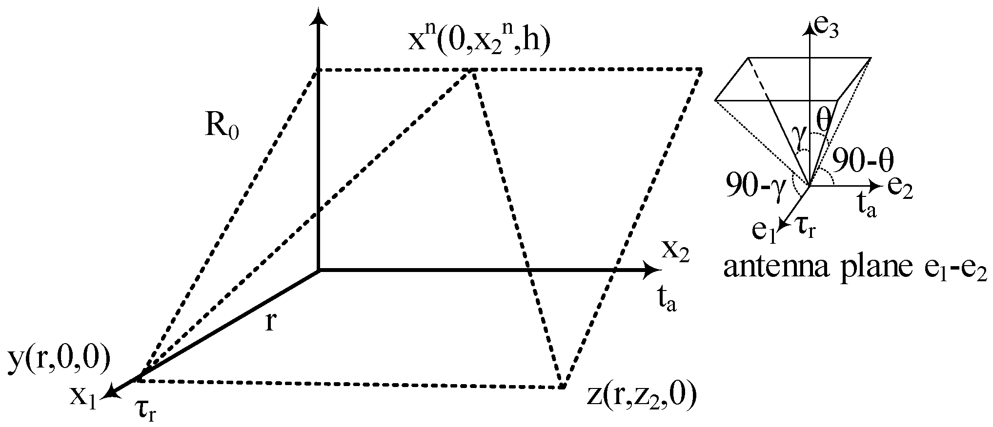
2.1. SAR Received Backscattered Signal Modeling

SAR is an active coherent microwave remote sensing device, the purpose of which is to form an image from the local interaction of a terrain illuminated by incidental electromagnetic waves. According to Figure 1, as the SAR platform flies along its designated path, known as the slow-time direction, the antenna radiates pulses of electromagnetic waves in a directed beam perpendicular to the flight direction, known as the fast-time. These waves scatter off the CTT and will be received and detected by the same antenna. The only processing performed on the received backscattered data is the striping of time-frame formatted signals, and re-assembling them into the synchronized unprocessed contiguous radar range lines, which are known as SAR raw data. The received backscattered signal depends on the fast-time (${\tau }_r$) and the position along the slow-time direction, $\mathrm{x}$, which results in a function of two variables based on Maxwell’s scalar wave equation [1,2,3]:

$$\left({\nabla }^2-\frac{1}{{\mathrm{c}}_0{}^2}{\partial }_{{\mathsf{\tau }}_{\mathrm{r}}}{}^2\right)\mathrm{U}\left({\mathsf{\tau }}_{\mathrm{r}},\mathrm{x}\right)=0$$

(1)

where, ${\mathrm{c}}_0$ is the speed of light. In the free space, the field ${\mathrm{G}}_0\left(\mathrm{t}-{\mathsf{\tau }}_{\mathrm{r}},\mathrm{x}-\mathrm{y}\right)$ at position $\mathrm{x}$ and time ${\mathsf{\tau }}_{\mathrm{r}}$ due to the delta function point scatterer at position $\mathrm{y}$ and time $\mathrm{t}$ will be driven as Equation (2):

$${\mathrm{G}}_0\left({\mathsf{\tau }}_{\mathrm{r}}-\mathrm{t},\mathrm{x}-\mathrm{y}\right)=\frac{\mathsf{\delta }({\tau }_r-\mathrm{t}-\left|\mathrm{x}-\mathrm{y}\right|/{\mathrm{c}}_0)}{4\mathsf{\pi }\left|\mathrm{x}-\mathrm{y}\right|}$$

(2)

This fields satisfies Equation (3):

$$\left({\nabla }^2-\frac{1}{{\mathrm{c}}_0{}^2}{\partial }_{{\mathsf{\tau }}_{\mathrm{r}}}{}^2\right){\mathrm{G}}_0\left({\mathsf{\tau }}_{\mathrm{r}}-\mathrm{t},\mathrm{x}-\mathrm{y}\right)=-\mathsf{\delta }\left({\mathsf{\tau }}_{\mathrm{r}}-\mathrm{t}\right)\mathsf{\delta }\left(\mathrm{x}-\mathrm{y}\right)$$

(3)

If the point scatterer at position $\mathrm{y}$ has the time history as Equation (4):

$$\mathrm{P}\left({\mathsf{\tau }}_{\mathrm{r}}\right)=\mathrm{A}\left({\mathsf{\tau }}_{\mathrm{r}}\right){\mathrm{e}}^{{\mathrm{i}\mathsf{\omega }}_0{\mathsf{\tau }}_{\mathrm{r}}}$$

(4)

then the resulting field ${\mathrm{U}}_{\mathrm{y}}\left({\mathsf{\tau }}_{\mathrm{r}},\mathrm{z}-\mathrm{y}\right)$ will satisfy Equation (5):

$$\left({\nabla }^2-\frac{1}{{\mathrm{c}}_0{}^2}{\partial }_{{\mathsf{\tau }}_{\mathrm{r}}}{}^2\right){\mathrm{U}}_{\mathrm{y}}\left({\mathsf{\tau }}_{\mathrm{r}},\mathrm{z}-\mathrm{y}\right)=-\mathrm{P}\left({\mathsf{\tau }}_{\mathrm{r}}\right)\mathsf{\delta }\left(\mathrm{z}-\mathrm{y}\right)$$

(5)

and is thus given by Equation (6):

$$\begin{array}{cc}\hfill {\mathrm{U}}_{\mathrm{y}}\left({\mathsf{\tau }}_{\mathrm{r}},\mathrm{z}\right)=\left({\mathrm{G}}_0\ast \mathrm{P}\right)& \left({\mathsf{\tau }}_{\mathrm{r}},\mathrm{z}-\mathrm{y}\right)\hfill \\ \hfill =& {{\displaystyle \int }}^{}\frac{\mathsf{\delta }\left({\mathsf{\tau }}_{\mathrm{r}}-\mathrm{t}-\left|\mathrm{z}-\mathrm{y}\right|/{\mathrm{c}}_0\right)}{4\mathsf{\pi }\left|\mathrm{z}-\mathrm{y}\right|}\mathrm{P}\left(\mathrm{t}\right)\mathrm{dt}=\frac{\mathrm{P}\left({\mathsf{\tau }}_{\mathrm{r}}-\left|\mathrm{z}-\mathrm{y}\right|/{\mathrm{c}}_0\right)}{4\mathsf{\pi }\left|\mathrm{z}-\mathrm{y}\right|}\hfill \\ \hfill =& \frac{\mathrm{A}\left({\mathsf{\tau }}_{\mathrm{r}}-\left|\mathrm{z}-\mathrm{y}\right|/{\mathrm{c}}_0\right)}{4\mathsf{\pi }\left|\mathrm{z}-\mathrm{y}\right|}{\mathrm{e}}^{{\mathrm{i}\mathsf{\omega }}_0\left({\mathsf{\tau }}_{\mathrm{r}}-\left|\mathrm{z}-\mathrm{y}\right|/{\mathrm{c}}_0\right)}\hfill \end{array}$$

(6)

If the length and width of the SAR antenna dimensions are denoted by $\mathrm{L}$ and $\mathrm{D}$, and the center of the antenna is denoted by $\mathrm{x}$, respectively, a point on the antenna can be written $\mathrm{y}=\mathrm{x}+\mathrm{q}$ where $\mathrm{q}$ is a vector from the center of the antenna to a point on the antenna, which is also introduced by Equation (7):

$$\mathrm{q}={\mathrm{s}}_1{\hat{\mathrm{e}}}_1+{\mathrm{s}}_2{\hat{\mathrm{e}}}_2$$

(7)

where, ${\hat{\mathrm{e}}}_1$ and ${\hat{\mathrm{e}}}_2$ are unit vectors along the width and length of the antenna. The vector ${\hat{\mathrm{e}}}_2$ points along the direction of the slow-time and ${\hat{\mathrm{e}}}_1$ is tilted with respect to the radiation direction or the fast-time. Considering point $\mathrm{z}$ far from the antenna, for which $\left|\mathrm{q}\right|\ll \left|\mathrm{z}-\mathrm{x}\right|$:

$$\left|\mathrm{z}-\mathrm{y}\right|=\left|\mathrm{z}-\mathrm{x}\right|-\widehat{\left(\mathrm{z}-\mathrm{x}\right)}\mathrm{q}+\mathrm{O}\left({\mathrm{L}}^2/\left|\mathrm{z}-\mathrm{x}\right|\right)$$

(8)

where the hat denotes a unit vector and $\widehat{\left(\mathrm{z}-\mathrm{x}\right)}$ is supposed as $\widehat{\left(\mathrm{L}\right)}$. With the help of Equation (6):

$${\mathrm{U}}_{\mathrm{y}}\left({\mathsf{\tau }}_{\mathrm{r}},\mathrm{z}\right)~\frac{\mathrm{A}\left({\mathsf{\tau }}_{\mathrm{r}}-\left|\mathrm{z}-\mathrm{x}\right|/{\mathrm{c}}_0+\widehat{\left(\mathrm{L}\right)}\mathrm{q}+\dots \right)}{4\mathsf{\pi }\left|\mathrm{z}-\mathrm{x}\right|}{\mathrm{e}}^{{\mathrm{i}\mathsf{\omega }}_0\left({\mathsf{\tau }}_{\mathrm{r}}-\left|\mathrm{z}-\mathrm{x}\right|/{\mathrm{c}}_0\right)}{\mathrm{e}}^{\mathrm{ik}\hat{\mathrm{L}}\mathrm{q}}$$

(9)

where $\mathrm{k}={\mathsf{\omega }}_0/{\mathrm{c}}_0$. If $\left|\mathrm{z}-\mathrm{x}\right|\gg \hat{\mathrm{L}}\mathrm{q}$ and A are assumed to be slowly varying, hence:

$${\mathrm{U}}_{\mathrm{y}}\left({\mathsf{\tau }}_{\mathrm{r}},\mathrm{z}\right)~\frac{\mathrm{P}\left({\mathsf{\tau }}_{\mathrm{r}}-\left|\mathrm{z}-\mathrm{x}\right|/{\mathrm{c}}_0\right)}{4\mathsf{\pi }\left|\mathrm{z}-\mathrm{x}\right|}{\mathrm{e}}^{\mathrm{ik}\hat{\mathrm{L}}\mathrm{q}}$$

(10)

Therefore, the far-field from the antenna is given by Equation (11):

$$\begin{array}{l}{\mathrm{U}}_{\mathrm{x}}^{\mathrm{in}}\left({\mathsf{\tau }}_{\mathrm{r}},\mathrm{z}\right)\\ ={{\displaystyle \int }}_{-\mathrm{L}/2}^{\mathrm{L}/2}{{\displaystyle \int }}_{-\mathrm{D}/2}^{\mathrm{D}/2}{\mathrm{U}}_{\mathrm{x}+{\mathrm{s}}_1\widehat{{\mathrm{e}}_1}+{\mathrm{s}}_2\widehat{{\mathrm{e}}_2}}\left({\mathsf{\tau }}_{\mathrm{r}},\mathrm{z}\right){\mathrm{ds}}_1{\mathrm{ds}}_2~{{\displaystyle \int }}_{-\mathrm{L}/2}^{\mathrm{L}/2}{{\displaystyle \int }}_{-\mathrm{D}/2}^{\mathrm{D}/2}\frac{\mathrm{P}\left({\mathsf{\tau }}_{\mathrm{r}}-\left|\mathrm{z}-\mathrm{x}\right|/{\mathrm{c}}_0\right)}{4\mathsf{\pi }\left|\mathrm{z}-\mathrm{x}\right|}{\mathrm{e}}^{\mathrm{ik}\hat{\mathrm{L}}.\left({\mathrm{s}}_1\widehat{{\mathrm{e}}_1}+{\mathrm{s}}_2\widehat{{\mathrm{e}}_2}\right)}{\mathrm{ds}}_1{\mathrm{ds}}_2\\ =\frac{\mathrm{P}\left({\mathsf{\tau }}_{\mathrm{r}}-\left|\mathrm{z}-\mathrm{x}\right|/{\mathrm{c}}_0\right)}{4\mathsf{\pi }\left|\mathrm{z}-\mathrm{x}\right|}\mathsf{\omega }\widehat{\left(\mathrm{L}\right)}\end{array}$$

(11)

where $\mathsf{\omega }\left(\hat{\mathrm{L}}\right)$ is the antenna radiation pattern and is directed perpendicular to the antenna plane (${\mathrm{e}}_1{\mathrm{e}}_2$) as Equation (12):

$$\mathsf{\omega }\left(\hat{\mathrm{L}}\right)=2\mathrm{D}\sin \mathrm{c}\left(\mathrm{k}\hat{\mathrm{L}}.{\mathrm{e}}_1\mathrm{D}/2\right)2\mathrm{L}\sin \mathrm{c}\left(\mathrm{k}\hat{\mathrm{L}}.{\mathrm{e}}_2\mathrm{L}/2\right)$$

(12)

The sinc function has its main peak at 0 and its zero at $\pi$. Therefore, the first zero of $\sin \mathrm{c}\left(\mathrm{k}\hat{\mathrm{L}}.{\mathrm{e}}_1\mathrm{D}/2\right)$ occurs when $\mathrm{k}\hat{\mathrm{L}}.{\mathrm{e}}_1\mathrm{D}/2=\mathsf{\pi }$. Using the fact that $2\mathsf{\pi }/\mathrm{k}$ is precisely the wavelength $\mathsf{\lambda }$, it can be written as $\hat{\mathrm{L}}.{\mathrm{e}}_2=\mathsf{\lambda }/\mathrm{L}$. In this case, the main lobe of the antenna beam pattern has an angular width of $2\mathsf{\lambda }/\mathrm{D}$ [1,3]. On the other hand, with the help of scattering theory, the linearized scattering model of Equation (1) can be considered as below [1]:

$$\mathsf{\Psi }\left({\mathsf{\tau }}_{\mathrm{r}},\mathrm{x}\right)={\mathsf{\Psi }}^{\mathrm{in}}\left({\mathsf{\tau }}_{\mathrm{r}},\mathrm{x}\right)+{\mathsf{\Psi }}^{\mathrm{sc}}\left({\mathsf{\tau }}_{\mathrm{r}},\mathrm{x}\right)$$

(13)

where:

$${\mathsf{\Psi }}^{\mathrm{sc}}\left({\mathsf{\tau }}_{\mathrm{r}},\mathrm{x}\right)={{\displaystyle \iint }}^{}{\mathrm{G}}_0\left({\mathsf{\tau }}_{\mathrm{r}}-\mathrm{t},\mathrm{x}-\mathrm{z}\right)\left(\frac{1}{{\mathrm{c}}_0^2}-\frac{1}{{\mathrm{c}}^2\left(\mathrm{z}\right)}\right){\partial }_{\mathrm{t}}^2{\mathsf{\Psi }}^{\mathrm{sc}}\left(\mathrm{t},\mathrm{z}\right){\mathrm{dtd}}^3\mathrm{z}$$

(14)

According to single scattering approximation, $\mathsf{\Psi }$ on the right side of Equation (13) is replaced by incident field ${\mathsf{\Psi }}^{\mathrm{in}}$ as Equation (15):

$$\begin{array}{cc}\hfill {\mathsf{\Psi }}^{\mathrm{sc}}\left({\mathsf{\tau }}_{\mathrm{r}},\mathrm{x}\right)\approx {\mathsf{\Psi }}^{\mathrm{B}}& \left({\mathsf{\tau }}_{\mathrm{r}},\mathrm{x}\right)\hfill \\ & ={{\displaystyle \iint }}^{}{\mathrm{G}}_0\left({\mathsf{\tau }}_{\mathrm{r}}-\mathrm{t},\mathrm{x}-\mathrm{z}\right)\left(\frac{1}{{\mathrm{c}}_0^2}-\frac{1}{{\mathrm{c}}^2\left(\mathrm{z}\right)}\right){\partial }_{\mathrm{t}}^2{\mathsf{\Psi }}^{\mathrm{in}}\left({\mathsf{\tau }}_{\mathrm{r}},\mathrm{x}\right){\mathrm{dtd}}^3\mathrm{z}\hfill \\ & ={{\displaystyle \int }}^{}\frac{\mathrm{V}\left(\mathrm{z}\right)}{4\mathsf{\pi }\left|\mathrm{x}-\mathrm{z}\right|}{\partial }_{{\mathsf{\tau }}_{\mathrm{r}}}^2{\mathsf{\Psi }}^{\mathrm{in}}\left({\mathsf{\tau }}_{\mathrm{r}}-\left|\mathrm{x}-\mathrm{z}\right|/{\mathrm{c}}_0,\mathrm{z}\right){\mathrm{d}}^3\mathrm{z}\hfill \end{array}$$

(15)

In the SAR remote sensing application, the antenna radiates a series of pulses in the form of Equation (11) as it moves along the flight track. Hence, if the platform is assumed to be located at position ${\mathrm{x}}^{\mathrm{n}}$ at time $\mathrm{nT}$, then the incident field is:

$${\mathsf{\Psi }}^{\mathrm{in}}\left(\mathrm{t},\mathrm{z}\right)={\displaystyle \sum }_{\mathrm{n}}{\mathsf{\Psi }}_{\mathrm{n}}^{\mathrm{in}}\left(\mathrm{t},\mathrm{z}\right)$$

(16)

$$\begin{array}{cc}\hfill {\mathsf{\Psi }}^{\mathrm{in}}\left(\mathrm{t},\mathrm{z}\right)={\mathrm{U}}_{{\mathrm{x}}^{\mathrm{n}}}^{\mathrm{in}}(\mathrm{t}& -\mathrm{nT},\mathrm{z})\hfill \\ & =\underset{\mathrm{antenna}}{\overset{}{{\displaystyle \iint }}}{\mathrm{U}}_{{\mathrm{x}}^{\mathrm{n}}+\mathrm{q}}\left(\mathrm{t}-\mathrm{nT},\mathrm{z}\right){\mathrm{d}}^2\mathrm{q}~\frac{\mathrm{P}\left(\mathrm{t}-\mathrm{nT}-\left|\mathrm{z}-{\mathrm{x}}^{\mathrm{n}}\right|/{\mathrm{c}}_0\right)}{4\mathsf{\pi }\left|\mathrm{z}-{\mathrm{x}}^{\mathrm{n}}\right|}\mathsf{\omega }\left(\widehat{\mathrm{z}-{\mathrm{x}}^{\mathrm{n}}}\right)\hfill \end{array}$$

(17)

where ${\mathsf{\Psi }}^{\mathrm{in}}\left(\mathrm{t},\mathrm{z}\right)$ is the $\mathrm{n}$th emission. With the help of Equation (17) and Equation (15), the scattered field due to the $\mathrm{n}$th emission at the center of the SAR antenna will be derived as Equation (18):

$${\mathrm{S}}_{\mathrm{n}}\left({\mathsf{\tau }}_{\mathrm{r}}\right)={\mathsf{\Psi }}_{\mathrm{n}}^{\mathrm{B}}\left({\mathsf{\tau }}_{\mathrm{r}}-\mathrm{nT},{\mathrm{x}}^{\mathrm{n}}\right)\approx -{{\displaystyle \int }}^{}\frac{{\mathsf{\omega }}_0^2\mathrm{P}({\mathsf{\tau }}_{\mathrm{r}}-\mathrm{nT}-2\left|\mathrm{z}-{\mathrm{x}}^{\mathrm{n}}\right|/{\mathrm{c}}_0)}{4\mathsf{\pi }\left|\mathrm{z}-{\mathrm{x}}^{\mathrm{n}}\right|}\mathsf{\omega }\left(\widehat{\mathrm{z}-{\mathrm{x}}^{\mathrm{n}}}\right){\mathrm{d}}^3\mathrm{z}$$

(18)

where $2\left|\mathrm{z}-{\mathrm{x}}^{\mathrm{n}}\right|/{\mathrm{c}}_0$ is the two-way travel time from the center of the antenna to the point $\mathrm{z}$ and factor $4\mathsf{\pi }\left|\mathrm{z}-{\mathrm{x}}^{\mathrm{n}}\right|$ in the denominator corresponding to the geometrical spreading of the spherical wave from the antenna and from point $\mathrm{z}$. It should be noted, in practice the factor of $\left|\mathrm{z}-{\mathrm{x}}^{\mathrm{n}}\right|$ will be replaced by the distance from $\mathrm{z}$ to the platform as ${\mathrm{R}}_0$, or the slantrange distance. For SAR image reconstruction, a match filter is applied to the received backscattered signal to from the 2-D raw data ${\mathrm{S}}_{\mathrm{n}}\left({\mathsf{\tau }}_{\mathrm{r}}\right)$ as Equation (19):

$${\mathrm{I}}_{\mathrm{n}}\left(\mathrm{y}\right)={{\displaystyle \int }}^{}\mathrm{P}\left({\mathsf{\tau }}_{\mathrm{r}}-\mathrm{nT}-2\left|\mathrm{y}-{\mathrm{x}}^{\mathrm{n}}\right|/{\mathrm{c}}_0\right){\ast \mathrm{S}}_{\mathrm{n}}\left({\mathsf{\tau }}_{\mathrm{r}}\right){\mathrm{d}\mathsf{\tau }}_{\mathrm{r}}$$

(19)

where the * denotes the complex conjugate. With the help of Equation (18) and interchange of the order of the integration, Equation (19) can be rewritten as Equation (20):

$${\mathrm{I}}_{\mathrm{n}}\left(\mathrm{y}\right)\approx {{\displaystyle \int }}^{}{\mathrm{W}}_{\mathrm{n}}\left(\mathrm{y},\mathrm{z}\right)\frac{-{\mathsf{\omega }}_0{}^2\mathrm{V}\left(\mathrm{z}\right)}{{\left(4{\mathsf{\pi }\mathrm{R}}_0\right)}^2}\mathrm{dz}$$

(20)

where:

$${\mathrm{W}}_{\mathrm{n}}\left(\mathrm{y},\mathrm{z}\right)=\mathsf{\omega }\left(\widehat{\mathrm{z}-{\mathrm{x}}^{\mathrm{n}}}\right){{\displaystyle \int }}^{}\mathrm{P}\left({\mathsf{\tau }}_{\mathrm{r}}-\mathrm{nT}-2\left|\mathrm{y}-{\mathrm{x}}^{\mathrm{n}}\right|/{\mathrm{c}}_0\right)\ast \mathrm{P}\left({\mathsf{\tau }}_{\mathrm{r}}-\mathrm{nT}-2\left|\mathrm{z}-{\mathrm{x}}^{\mathrm{n}}\right|/{\mathrm{c}}_0\right)\mathrm{d}{\mathsf{\tau }}_{\mathrm{r}}$$

(21)

This represents the point spread function (PSF) of one observation of the SAR sensor, which results in an image. The key concept of the SAR sensor is to improve this PSF with the help of summing over $\mathrm{n}$. Hence, by combining information from multiple observations or simply multiple looks:

$$\mathrm{I}\left(\mathrm{y}\right)={\displaystyle \sum }_{\mathrm{n}}{\mathrm{I}}_{\mathrm{n}}\left(\mathrm{y}\right)\approx {{\displaystyle \int }}^{}\mathrm{W}\left(\mathrm{y},\mathrm{z}\right)\frac{-{\mathsf{\omega }}_0{}^2\mathrm{V}\left(\mathrm{z}\right)}{{\left(4{\mathsf{\pi }\mathrm{R}}_0\right)}^2}\mathrm{dz}$$

(22)

where the PSF is calculated as:

$$\mathrm{W}\left(\mathrm{y},\mathrm{z}\right)={\displaystyle \sum }_{\mathrm{n}}{\mathrm{W}}_{\mathrm{n}}\left(\mathrm{y},\mathrm{z}\right)$$

(23)

This point spread function is called the SAR ambiguity function (AF) of the transmitted waveform.

2.2. Multiplicative Speckle Noise Behaviroal Formulation and Modeling

The two basic principle features of an SAR system are the resolution of the image and the spatial resolution or the system resolution. The system resolution directly affects the image resolution, while the image resolution is completely dependent on the quality of the received backscattered data and its pertinent information. A serious difficulty in exploiting and analyzing the raw data is the presence of coherent multiplicative noise that inherently exists in these images, and is called speckle. According to Equations (4) and (16), in the case of electromagnetic waves backscattering from the surface to the SAR, both the phase $\mathsf{\phi }\left(\mathrm{x},\mathrm{y}\right)$ and the amplitude $\mathrm{A}\left(\mathrm{x},\mathrm{y}\right)$ of the signal are changed. These changes are due to the different physical properties of the CTT, as well as the deviations of the trajectory from the nominal or the attitude and forward velocity variations, which mostly happen during the observation time, as shown in Figure 1. In other words, these echo data are not coherent signal anymore because of atmospheric turbulence and radiometric errors that can easily affect the phase history of the raw data within the plane of the antenna $\left({\mathrm{e}}_1{\mathrm{e}}_2\right)$ [24,25]. In practice, phase errors are residue phases that degrade the standard level of the received signal components and make them not coherent anymore for the purpose of processing. Therefore, any time the SAR collects the complex value of ${\mathrm{Ae}}^{\mathrm{j}\mathsf{\phi }}$ from the distributed point scatterers within the terrain, the 2-D signals add coherently as constructive or destructive, depending on the relative phase; this is usually referred to as multiplicative speckle noise. In other words, speckles reduce the image quality like noise, but not randomly. This comes from the backscattering of many point scatterers within the CTT, and presents as image pixel anomalies. According to Equation (17), every pixel in an SAR image results from the backscattered wave of a large number of point scatterers located in one resolution cell, and this can be modeled as a complex value of Equation (4):

$${\mathrm{Ae}}^{\mathrm{j}\mathsf{\phi }}={\displaystyle \sum }_{\mathrm{i}=1}^{\mathrm{N}}{\mathrm{A}}_{\mathrm{i}}{\mathrm{e}}^{{\mathrm{j}\mathsf{\phi }}_{\mathrm{i}}}$$

(24)

where ${\mathrm{A}}_{\mathrm{i}}$ and ${\mathsf{\phi }}_{\mathrm{i}}$ are the individual amplitude and phase of the backscattering, while N is the total number of scatterers within the resolution cell. The summation is over the number of point scatterers located in one cell illuminated by the electromagnetic wave, while different weights in the form of PSF and Equation (23) will be implemented. ${\mathrm{A}}_{\mathrm{i}}$ and ${\mathsf{\phi }}_{\mathrm{i}}$ are unobservable because the individual scatters are much smaller than the resolution cell. Hence, the speckle can be formulated as a multiplicative model of pixel anomaly:

$$\mathrm{O}=\mathrm{I}·\mathrm{Y}$$

(25)

where $\mathrm{O}$ is the observation result, $\mathrm{I}$ is the average CTT backscattered intensity, and $\mathrm{Y}$ is the noise intensity. $\mathrm{I}$ and $\mathrm{Y}$ are considered as two independent random variables. In the case of multiplicative noise demodulation modeling, the observed in-phase and quadrature-phase components of the speckle noise ${\mathrm{y}}_1=\mathrm{Acos}\left(\mathsf{\phi }\right)$ and ${\mathrm{y}}_2=\mathrm{Asin}\left(\mathsf{\phi }\right)$ are assumed to be identical distributed Gaussian random complex variables with zero means and a variance of ½ [3]. Consequently, the joint probability density function (PDF) can be written as:

$${\mathrm{p}}_{{\mathrm{y}}_1,{\mathrm{y}}_2}\left({\mathrm{y}}_1,{\mathrm{y}}_2\right)=\frac{1}{\mathsf{\pi }}\exp \left(-\left({\mathrm{y}}_1^2+{\mathrm{y}}_2^2\right)\right)$$

(26)

where the phase $\mathsf{\phi }$ is assumed to be uniformly distributed. On the other side, the amplitude $\mathrm{A}$ has a Rayleigh distribution, as:

$${\mathrm{p}}_{\mathrm{A}}\left(\mathrm{y}\right)=2\mathrm{y}\exp \left(-{\mathrm{y}}^2\right)\mathrm{y}\ge 0$$

(27)

with the mean value of $\sqrt{\mathsf{\pi }}/2$ and standard deviation of $\sqrt{1-\mathsf{\pi }/4}$. On the other hand, the standard deviation divided by the mean is $\sqrt{4/\mathsf{\pi }-1}$. The observed intensity has a negative exponential distribution, as:

$${\mathrm{p}}_{\mathrm{I}}\left(\mathrm{y}\right)=2\mathrm{y}\exp \left(-\mathrm{y}\right)\mathrm{y}\ge 0$$

(28)

where the mean value and standard deviation are both in unity. The decibel image as the logarithmic transformed intensity is derived as:

$${\mathrm{p}}_{\mathrm{I}}\left(\mathrm{y}\right)={\mathrm{e}}^{\mathrm{y}}\exp \left(-{\mathrm{e}}^{\mathrm{y}}\right)$$

(29)

where the mean and variance are −0.57 and ${\mathsf{\pi }}^2/6$. If the number of observations is K, the average intensity of the K-observation can be written as:

$${\mathrm{Y}}_{\mathrm{O}}=\frac{{{\displaystyle \sum }}_{\mathrm{i}=1}^{\mathrm{K}}{\mathrm{Y}}_{\mathrm{O}}^{\mathrm{i}}}{\mathrm{K}}$$

(30)

where ${\mathrm{Y}}_{\mathrm{O}}^{\mathrm{i}}$ is the independent single-observation intensity with a negative exponential distribution. In the case of multi-observation of ${\mathrm{Y}}_{\mathrm{O}}$, the model will be rewritten as:

$${\mathrm{p}}_{\mathrm{O}}\left(\mathrm{y}\right)=\frac{{\mathrm{K}}^{\mathrm{K}}}{\mathsf{\Gamma }\left(\mathrm{K}\right)}{\mathrm{y}}^{\mathrm{K}-1}\exp \left(-\mathrm{Ky}\right)\mathrm{y},\mathrm{K}>0$$

(31)

where K is the multi-observation number of ${\mathrm{Y}}_{\mathrm{O}}$ with the mean and variance of unity and $1/\mathrm{K}$. For a single look image, the amplitude obeys Rayleigh PDF. This multiplicative behavior on the basis of signal characteristics is generated by the interaction of the reflected waves from various independent scatterers within a resolution cell. In total, the characteristics of the multiplicative speckle noise in SAR imagery are very different from those found in the other sensors, which might contain additive white Gaussian noise. Hence, the formulated SAR multiplicative speckle noise has an asymmetrical PDF and the Gamma distribution, which is considered completely signal dependent based on the phase distribution, the amplitude distribution, the intensity distribution, and the observation number. On the other hand, according to the characteristics of speckle noise, the coefficients are being modulated by the characteristic of the noise in a manner that is proportional to the target mean backscattering coefficients. In other words, extracting the coefficients of speckle noise can be evaluated based on their expectation and variance, despite their limitations while dealing with random entities within the terrain. Considering ${\mathrm{O}}_1$ and ${\mathrm{O}}_2$ as two adjacent pixels in a SAR observation:

$$\begin{gathered} {\mathrm{O}}_1={\mathrm{c}}_1{\mathrm{Y}}_1 \\ {\mathrm{O}}_2={\mathrm{c}}_2{\mathrm{Y}}_2 \end{gathered}$$

(32)

where ${\mathrm{c}}_1$ and ${\mathrm{c}}_2$ are constants and ${\mathrm{Y}}_1$ and ${\mathrm{Y}}_2$ are independent random variables with identical probability, according to the general Gamma distribution $\mathsf{\Gamma }\left(\mathrm{n},\mathsf{\lambda }\right)$. Therefore, the PDF can be modeled as:

$$\mathrm{p}\left(\mathrm{y}\right)=\frac{{\mathsf{\lambda }}^{\mathrm{n}}}{\left(\mathrm{n}-1\right)!}{\mathrm{y}}^{\mathrm{n}-1}\exp \left(-\mathsf{\lambda }\mathrm{y}\right)$$

(33)

If $\mathrm{a}$ and $\mathrm{b}$ are considered as the backscattered intensities, the two adjacent pixels ${\mathrm{O}}_1$ and ${\mathrm{O}}_2$ belong to a homogenous region in case of $\mathrm{a}$ equals $\mathrm{b}$. Otherwise, ${\mathrm{O}}_1$ and ${\mathrm{O}}_2$ are located in two different regions. If $\mathrm{a}\ne 0$ and $\mathrm{b}\ne 0$, ${\mathrm{O}}_1$ and ${\mathrm{O}}_2$ follow the general Gamma distribution $\mathsf{\Gamma }\left(\mathrm{n},\mathsf{\lambda }/\mathrm{a}\right)$ and $\mathsf{\Gamma }\left(\mathrm{n},\mathsf{\lambda }/\mathrm{b}\right)$, with the form below:

$$\begin{gathered} {\mathrm{p}}_{{\mathrm{O}}_1}\left(\mathrm{x}\right)=\frac{{\mathsf{\lambda }}^{\mathrm{n}}}{\mathrm{a}\left(\mathrm{n}-1\right)!}{\left(\frac{\mathrm{x}}{\mathrm{a}}\right)}^{\mathrm{n}-1}\exp \left(\frac{-\mathsf{\lambda }}{\mathrm{a}}\mathrm{x}\right)\mathrm{where}\mathrm{x},\mathrm{n}\ge 0,\mathrm{and} \\ {\mathrm{p}}_{{\mathrm{O}}_2}\left(\mathrm{y}\right)=\frac{{\mathsf{\lambda }}^{\mathrm{n}}}{\mathrm{b}\left(\mathrm{n}-1\right)!}{\left(\frac{\mathrm{x}}{\mathrm{b}}\right)}^{\mathrm{n}-1}\exp \left(\frac{-\mathsf{\lambda }}{\mathrm{b}}\mathrm{y}\right)\mathrm{where}\mathrm{y},\mathrm{n}\ge 0 \end{gathered}$$

(34)

The property of ${\mathrm{O}}_1-{\mathrm{O}}_2$ is the basis for the development of the multiplicative speckle property and its complex modeling. If the cumulative distribution function of ${\mathrm{O}}_1-{\mathrm{O}}_2$ is defined as:

$$\mathrm{P}({\mathrm{O}}_1-{\mathrm{O}}_2<\mathrm{t})={{\displaystyle \iint }}_{\mathrm{x}-\mathrm{y}\le \mathrm{t}}{\mathrm{p}}_{{\mathrm{O}}_1}\left(\mathrm{x}\right){\mathrm{p}}_{{\mathrm{O}}_2}\left(\mathrm{y}\right)\mathrm{dxdy}$$

(35)

This will result in:

$$\mathrm{P}({\mathrm{O}}_1-{\mathrm{O}}_2<\mathrm{t})=\{\begin{array}{c}\exp \left(-\frac{\mathsf{\lambda }}{\mathrm{b}}\left|\mathrm{t}\right|\right)\frac{{\mathsf{\lambda }}^{\mathrm{n}}}{{\mathrm{a}}^{\mathrm{n}}\left(\mathrm{n}-1\right)!}{\displaystyle \sum }_{\mathrm{i}=0}^{\mathrm{n}-1}\frac{{\mathsf{\lambda }}^{\mathrm{i}}}{{\mathrm{b}}^{\mathrm{i}}}\left[{\displaystyle \sum }_{\mathrm{j}=0}^{\mathrm{i}}\frac{{\left|\mathrm{t}\right|}^{\mathrm{i}-\mathrm{j}}}{\mathrm{j}!\left(\mathrm{i}-\mathrm{j}\right)!}\frac{\left(\mathrm{n}+\mathrm{j}-1\right)!}{{\left(\frac{\mathsf{\lambda }}{\mathrm{a}}+\frac{\mathsf{\lambda }}{\mathrm{b}}\right)}^{\mathrm{n}+\mathrm{j}}}\right]\mathrm{t}\le 0\\ 1-\exp \left(-\frac{\mathsf{\lambda }}{\mathrm{b}}\left|\mathrm{t}\right|\right)\frac{{\mathsf{\lambda }}^{\mathrm{n}}}{{\mathrm{a}}^{\mathrm{n}}\left(\mathrm{n}-1\right)!}{\displaystyle \sum }_{\mathrm{i}=0}^{\mathrm{n}-1}\frac{{\mathsf{\lambda }}^{\mathrm{i}}}{{\mathrm{b}}^{\mathrm{i}}}\left[{\displaystyle \sum }_{\mathrm{j}=0}^{\mathrm{i}}\frac{{\left|\mathrm{t}\right|}^{\mathrm{i}-\mathrm{j}}}{\mathrm{j}!\left(\mathrm{i}-\mathrm{j}\right)!}\frac{\left(\mathrm{n}+\mathrm{j}-1\right)!}{{\left(\frac{\mathsf{\lambda }}{\mathrm{a}}+\frac{\mathsf{\lambda }}{\mathrm{b}}\right)}^{\mathrm{n}+\mathrm{j}}}\right]\mathrm{t}>0\end{array}$$

(36)

The PDF of ${\mathrm{O}}_1$ − ${\mathrm{O}}_2$ can be derived as:

$${\mathrm{p}}_{{\mathrm{O}}_1-{\mathrm{O}}_2}\left(\mathrm{y}\right)=\frac{\exp \left(-\frac{\mathsf{\lambda }}{\mathrm{b}}\left|\mathrm{y}\right|\right)}{\left(\mathrm{n}-1\right)!}{\left(\frac{\mathsf{\lambda }}{\mathrm{a}}\right)}^{\mathrm{n}}{\left(\frac{\mathsf{\lambda }}{\mathrm{b}}\right)}^{\mathrm{n}}\left[{\displaystyle \sum }_{\mathrm{j}=0}^{\mathrm{n}-1}\frac{\left(\mathrm{n}+\mathrm{j}-1\right)!}{\mathrm{j}!\left(\mathrm{n}-\mathrm{j}-1\right)!{\left(\frac{\mathsf{\lambda }}{\mathrm{a}}+\frac{\mathsf{\lambda }}{\mathrm{b}}\right)}^{\mathrm{n}+\mathrm{j}}}{\left|\mathrm{y}\right|}^{\mathrm{n}-\mathrm{j}-1}\right]$$

(37)

Hence, the moments of ${\mathrm{O}}_1-{\mathrm{O}}_2$ can be driven by:

$$\begin{gathered} \left[{\mathrm{x}}^{\mathrm{k}}\right]=\frac{2}{\left(\mathrm{n}-1\right)!}{\left(\frac{\mathsf{\lambda }}{\mathrm{a}}\right)}^{\mathrm{n}}{\left(\frac{\mathsf{\lambda }}{\mathrm{b}}\right)}^{\mathrm{n}}\left[{{\displaystyle \sum }}_{\mathrm{j}=0}^{\mathrm{n}-1}\frac{\left(\mathrm{n}+\mathrm{j}-1\right)!\left(\mathrm{i}+\mathrm{n}-\mathrm{j}-1\right)!}{\mathrm{j}!\left(\mathrm{n}-\mathrm{j}-1\right)!{\left(\frac{\mathsf{\lambda }}{\mathrm{a}}+\frac{\mathsf{\lambda }}{\mathrm{b}}\right)}^{\mathrm{n}+\mathrm{j}}}{\left|\frac{\mathrm{b}}{\mathsf{\lambda }}\right|}^{\mathrm{i}+\mathrm{n}-\mathrm{j}}\right]\mathrm{if}\mathrm{i}\mathrm{is}\mathrm{even} \\ \mathrm{E}\left[{\mathrm{x}}^{\mathrm{k}}\right]=0\mathrm{if}\mathrm{i}\mathrm{is}\mathrm{odd} \end{gathered}$$

(38)

To model the behavior of the speckle noise based on complex modeling, let $\mathrm{a}=\mathrm{b}=1$. Hence, Equation (37) will be rewritten as:

$${\mathrm{p}}_{{\mathrm{O}}_1-{\mathrm{O}}_2}\left(\mathrm{y}\right)=\frac{\exp \left(-\mathsf{\lambda }\left|\mathrm{y}\right|\right)}{\left(\mathrm{n}-1\right)!}{\left(\mathsf{\lambda }\right)}^{2\mathrm{n}}\left[{\displaystyle \sum }_{\mathrm{j}=0}^{\mathrm{n}-1}\frac{\left(\mathrm{n}+\mathrm{j}-1\right)!}{\mathrm{j}!\left(\mathrm{n}-\mathrm{j}-1\right)!{\left(2\mathsf{\lambda }\right)}^{\mathrm{n}+\mathrm{j}}}{\left|\mathrm{y}\right|}^{\mathrm{n}-\mathrm{j}-1}\right]$$

(39)

Equations (37) and (39), which are a combination of the exponential function and polynomial, are very important for behavioral modeling of multiplicative speckle noise. The aforementioned distribution and its corresponding statistical features on the basis of the phase distribution, the amplitude distribution, the intensity distribution, and the observation number are used for complex modeling.

According to the above distribution and complex modeling of the multiplicative speckle noise, power spectral density function (PSD) modeling is considered the best possible option to investigate the effects of the speckle presence within SAR images. The PSD, as an objective quality assessment metric, measures the intensity of the joint pixels as a function of frequency and shows at which frequencies the intensity variations are stronger, and at which frequencies variations are weak. According to the above modeling, pixels and their statistical distribution based on amplitude, phase, and intensity play a key role for complex speckle PSD modeling.

Figure 1 presents the reference SAR image sample and the resulting PSD function modeling. The PSD modeling is based on the pixel intensities and their distribution statistics, which are assigned and presented in the frequency domain. The results show that, in the case of the reference SAR image consisting of non-overlapping pixels that are not reduced to the replications of a specific statistics, lower frequencies with significant variance in the distribution of pixels have peaks in PSD modeling that can be distinguished in Figure 2b. The peaks in the PSD function modeling present the statistics of the main entity of the texture, and are also presented in Figure 2c,d. The difference between Figure 2b–d is based on their pixel statistics estimation and distribution modeling. Figure 2c shows the case of the speckle reduction technique on the basis of filter application, and 2d shows the case of noise-free supposition. The results show that speckle presence can directly affect the pixel statistics and distribution, such as the phase, the amplitude, and the intensity. On the contrary, and in the case of speckle PSD function modeling, the pixel statistics and distribution will be completely different from the reference image statistics. According to Equations (32)–(39), the results of PSD function modeling for embedded speckle within the reference image are presented in Figure 2e. Figure 2e shows that the speckle behavior, as an overlapping structure which occupies approximately the entire spatial area of the SAR image, has several high-frequency peaks which are close in terms of their spatial locations. Figure 2e also shows that, in comparison to the main texture of the reference image, the speckle has a replication structure on the basis of its distribution and statistics. In other words, speckle with significant effects on the amplitude, phase and the intensity can be modeled as a high-frequency replication structure of the PSD function. As a result, multiplicative speckle noise can be named as high-frequency multiplicative speckle (HMS) noise hereafter. From Figure 2 it is also deduced that HMS noise not only affects the maximum value of the PSD function, but also affects the uniformity of the texture. The results show that real reference SAR imagery and noise-free conditions have a total 4 dB difference in PSD function magnitude, while the HMS has a maximum 0.4 dB adverse effect on the PSD magnitude.

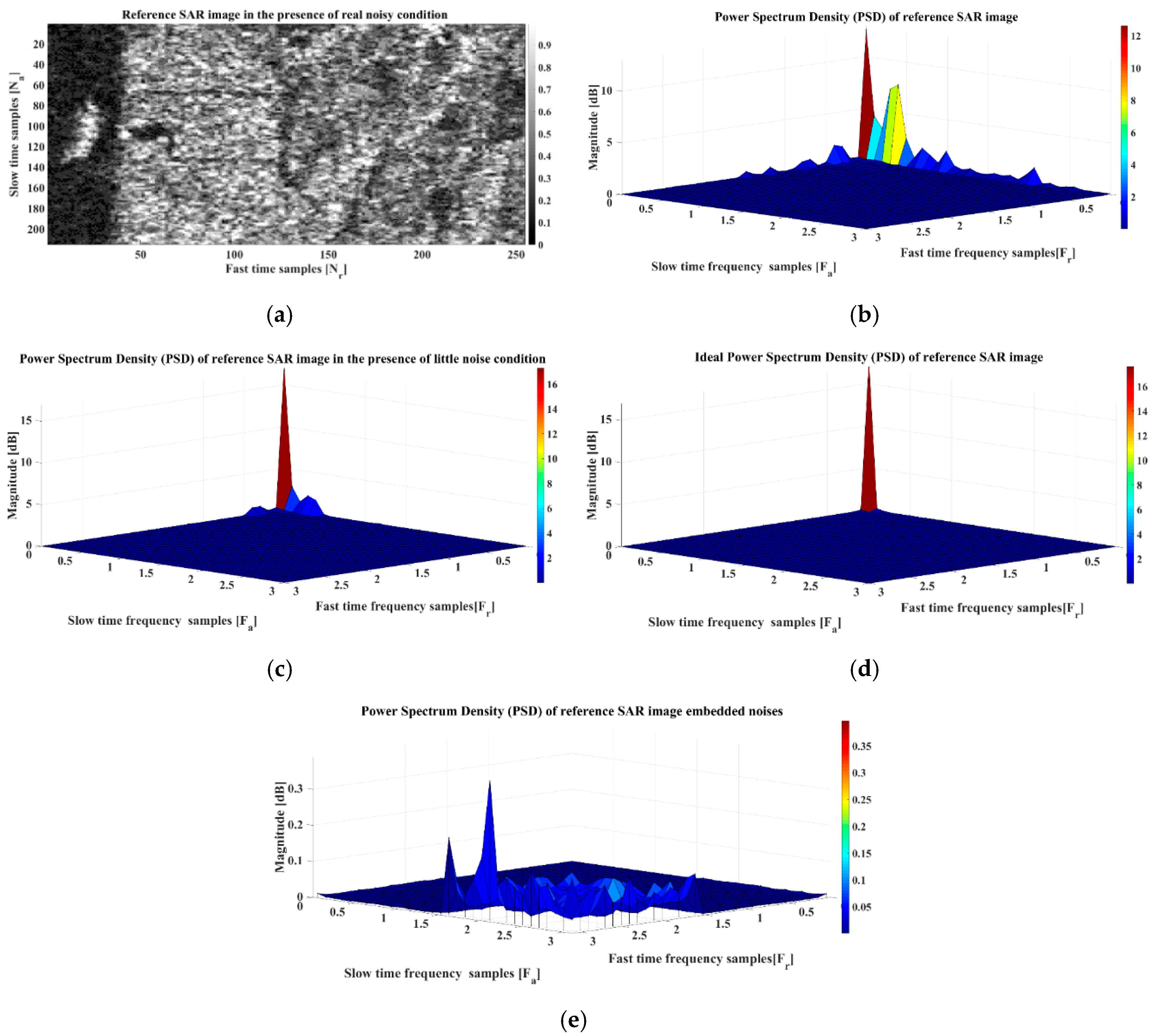
2.3. De-Speckled Image HMS Noise Behavioral Modeling

In total, the non-uniform antenna pattern illumination, possible receiver gain changes, loss effects, scattering abnormalities phenomenon, and so forth are the source of HMS noise, which will affect the pixel statistics and their inherent distribution, such as their amplitude, phase and the intensity, in a destructive or constructive manner [21,24,25]. According to these patterns of constructive and destructive interference, HMS noise can also be suppressed with the help of de-speckling filters. During the past decades, by considering the variance of backscatter amplitude, many de-speckling filters have been proposed for HMS noise reduction [25]. These filters can be divided into two groups—transform domain and spatial domain—which are usually designed to cope with the variation of pixel amplitude. In the case of spatial filters, they use local pixel intensity statistics to adjust the amount of noise removal in a certain threshold, and perform acceptably in homogeneous regions, but in heterogeneous regions they cause loss of detail [25]. Due to the lack of investigation on spatial domain filter application and suitable selection, this section will present the PSD function modeling of the de-speckled images and their embedded HMS noise for further comparison. Therefore, taking into consideration the implementation of seven different spatial de-speckling filters—Frost, Gamma, Kuan, Lee, Lee sigma, Local adaptive median and Local sigma—on the same reference SAR image and modeling their PSD function may be a good technique to evaluate their noise suppression ability while dealing with HMS noise. The results are shown in Figure 3.

As can be deduced from the PSD modeling results in Figure 3b,d,f,h,j,l,n, the simulated PSD functions are not only different in the uniformity of the peak distribution, but also vary in terms of their magnitude. The results show that, despite using the same SAR image with a similar texture, different PSD models under different spatial de-speckling filters might result. In this case, the minimum quality and lowest magnitude belongs to the Lee sigma filter with 12.2 dB magnitude, while the best performance belongs to the Gamma filter with more than 25.5 dB magnitude. This shows that, if the distribution of the peaks within the PSD modeling is minor and their concentration has a large uniform magnitude, this is a sign of acceptable de-speckling. According to Figure 3,

Table 1. PSD modeling results after HMS suppression.

Column	De-Speckling Filter	Value
1	Gamma	25.5 dB
2	Lee	22 dB
3	Local sigma	20.5 dB
4	Frost	18.4 dB
5	Local adaptive median	14.4 dB
6	Kuan	14.1 dB
7	Lee sigma	12.2 dB

presents the ranking of the aforementioned filters based on their peak values. Due to limitations of the filters in terms of the complete removal of the HMS, the presence of fluctuation in the PSD modeling is normal. Figure 4 illustrates the difference between the PSD modeling of the reference SAR image in Figure 2b, and their counterparts in Figure 3. The results verify that de-speckled images have different HMS pattern within the texture, and each spatial filter has its own specifications to reduce the level of the HMS.

According to Figure 3 and Figure 4, besides the ability of spatial filters to achieve HMS suppression, the effect of the spatial filter application on the texture is also a key concept. Hence, similar to the PSD modeling of the HMS suppression, PSD modeling of the pure HMS presence within the texture is helpful. The results of this are shown in Figure 5 and listed in

Table 2. Residue HMS presence evaluation after de-speckling implementation.

Column	De-Speckling Filter	Value
1	Local sigma	0.14 dB
2	Kuan	0.14 dB
3	Local adaptive median	0.18 dB
4	Lee sigma	0.31 dB
5	Frost	0.36 dB
6	Lee	0.60 dB
7	Gamma	0.62 dB

. As can be deduced, the shape, the distribution and the peaks of the HMS presence within the texture after de-speckling filter implementation are completely different. The minimum presence level of HMS is 0.14 dB, which is observed when the Local sigma has been implemented, and the maximum presence value is 0.62 dB for the Gamma de-speckling filter implementation.

From Figure 5, it can be deduced that the Kuan and Local sigma filters have the least amount of residue HMS in the texture after de-speckling, while according to Table 1, their performance in HMS suppression was just moderate. It also verifies that spatial de-speckling filter implementation not only affects the texture consistency after HMS removal, but also changes the HMS distribution and statistics based on amplitude, intensity, and phase. In other words, there has always been residue HMS with non-specific patterns within the texture after de-speckling.

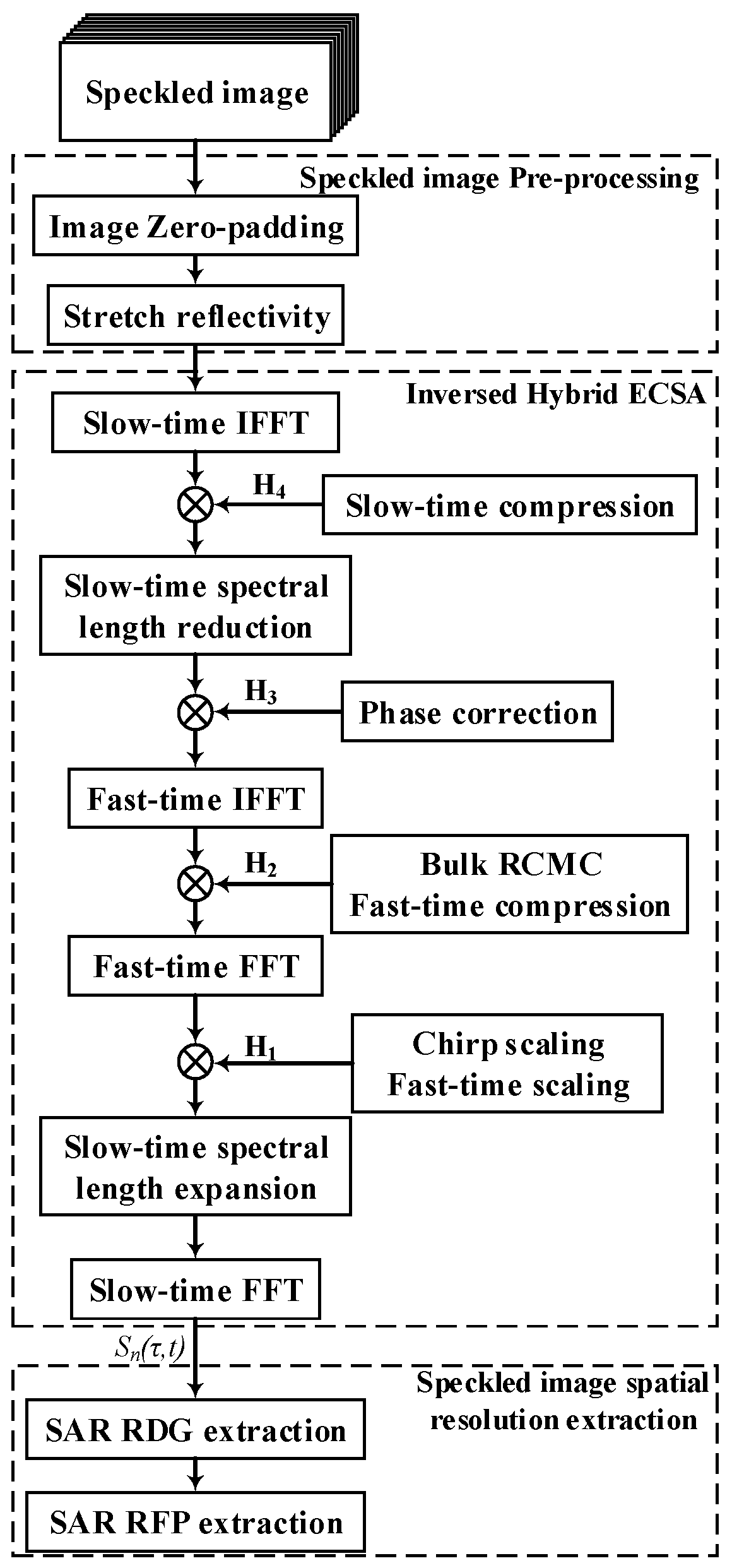
2.4. HMS System Resolution Extraction Method Concept

According to Figure 1, suppose the SAR platform flies in the direction of the slow-time and the point scatterer is located within the CTT with an initial slant range of ${\mathrm{R}}_0$ from the sensor. According to Equations (18) and (24), the received 2-D backscattered pulse from the point scatterer in the case of linear frequency modulation waveform can be expressed as (40) [3]:

$$\begin{array}{c}{\mathrm{S}}_{\mathrm{n}}({\mathsf{\tau }}_{\mathrm{r}},{\mathrm{t}}_{\mathrm{a}})=\mathrm{A}.{\mathrm{w}}_{{\mathsf{\tau }}_{\mathrm{r}}}\left({\mathsf{\tau }}_{\mathrm{r}}-2\mathrm{R}\left({\mathrm{t}}_{\mathrm{a}}\right)/{\mathrm{c}}_0\right){\mathrm{w}}_{{\mathrm{t}}_{\mathrm{a}}}\left({\mathrm{t}}_{\mathrm{a}}\right)\times \cos \{2{\mathsf{\pi }\mathrm{k}}_0\left({\mathsf{\tau }}_{\mathrm{r}}-2\mathrm{R}\left({\mathrm{t}}_{\mathrm{a}}\right)/{\mathrm{c}}_0\right)+\\ {\mathsf{\pi }\mathrm{K}}_{\mathrm{r}}{\left({\mathsf{\tau }}_{\mathrm{r}}-2\mathrm{R}\left({\mathrm{t}}_{\mathrm{a}}\right)/{\mathrm{c}}_0\right)}^2+\mathsf{\psi }\}\end{array}$$

(40)

where, ${\mathrm{t}}_{\mathrm{a}}$ is the slow-time, ${\mathsf{\tau }}_{\mathrm{r}}$ is the fast-time, ${\mathrm{S}}_{\mathrm{n}}$(${\mathsf{\tau }}_{\mathrm{r}}$,${\mathrm{t}}_{\mathrm{a}}$) is the received 2-D backscattered signal from the scatterer, $\mathrm{A}$ is the backscattering coefficient, ${\mathrm{w}}_{{\mathsf{\tau }}_{\mathrm{r}}}(.)$ is the received pulse envelope in fast-time, ${\mathrm{w}}_{{\mathrm{t}}_{\mathrm{a}}}$ is the received pulse envelope in slow-time, ${\mathrm{k}}_0$ is the carrier frequency, ${\mathrm{K}}_{\mathrm{r}}$ is the chirp rate, and ${\mathrm{c}}_0$ is the speed of light. The variable of $\mathsf{\psi }$ is accounted for in the phase change problem during the reception procedure. According to Equations (24)–(39), the received echo is a coherent signal while being backscattered from the CTT due to the possible phase changes of $\mathsf{\psi }$ within the phase history [24]. The phase changes of the raw data, as mentioned in the previous sections, are considered as the source of HMS presence within the texture. The purpose of SAR system resolution extraction is twofold. The first, namely the RDG extraction, allows us to evaluate the HMS effects on the backscattering behavior of the CTT while it is being being backscattered to the sensor as ${\mathrm{S}}_{\mathrm{n}}$ (${\mathsf{\tau }}_{\mathrm{r}}$, ${\mathrm{t}}_{\mathrm{a}}$), in the form of the received backscattered signal. The second, namely the RFP extraction, carries out SAR frequency profile analysis based on the HMS presence within the ${\mathrm{S}}_{\mathrm{n}}$ (${\mathsf{\tau }}_{\mathrm{r}}$, ${\mathrm{t}}_{\mathrm{a}}$), while being arranged and reassembled into baseband contiguous radar range lines in the form of $\mathsf{\psi }$ interferences. The block diagram of the complete aforementioned hybrid-domain IFA based on the extended chirp scaling algorithm for the purpose of system resolution extraction is shown in Figure 6. The structure of the algorithm is prepared based on the principle of stationary phase (POSP) [3]. With the help of POSP, the corresponding baseband signal of Equation (40) is expressed as Equation (41):

$$\begin{array}{cc}\hfill {\mathrm{S}}_{\mathrm{BB}}\left({\mathsf{\tau }}_{\mathrm{r}},{\mathrm{f}}_{{\mathrm{t}}_{\mathrm{a}}}\right)={\mathrm{W}}_{{\mathsf{\tau }}_{\mathrm{r}}}& \left({\mathsf{\tau }}_{\mathrm{r}}-2\mathrm{R}\left({\mathrm{f}}_{{\mathrm{t}}_{\mathrm{a}}},{\mathrm{r}}_0\right)/{\mathrm{c}}_0\right).{\mathrm{W}}_{{\mathrm{t}}_{\mathrm{a}}}\left({\mathrm{r}}_0{\mathsf{\lambda }\mathrm{f}}_{{\mathrm{t}}_{\mathrm{a}}}/2{\mathrm{v}}^2\mathsf{\beta }\left({\mathrm{f}}_{\mathrm{t}}\right)\right)\hfill \\ & \times \exp \left[-j4\pi f_0{r}_0\beta \left(f_{t_a}\right)/{\mathrm{c}}_0\right]\exp \left[\mathrm{j}\mathsf{\pi }{\mathrm{K}}_{\mathrm{r}}\left({\mathrm{f}}_{{\mathrm{t}}_{\mathrm{a}}},{\mathrm{r}}_0\right)({\mathsf{\tau }}_{\mathrm{r}}-2\mathrm{R}{\left({\mathrm{f}}_{{\mathrm{t}}_{\mathrm{a}}},{\mathrm{r}}_0\right)}^2\right]\hfill \end{array}$$

(41)

where v is the relative velocity between the platform and the CTT, $\mathsf{\lambda }$ is the radar wavelength, ${\mathrm{r}}_0$ is the distance of the closest approach, ${\mathrm{f}}_{{\mathrm{t}}_{\mathrm{a}}}$ is the frequency corresponding to slow-time, $\mathrm{R}\left({\mathrm{f}}_{{\mathrm{t}}_{\mathrm{a}}},{\mathrm{r}}_0\right)$ is the range migration in the time-frequency domain, and ${\mathrm{K}}_{\mathrm{r}}\left({\mathrm{f}}_{{\mathrm{t}}_{\mathrm{a}}},{\mathrm{r}}_0\right)$ is the modulation rates of chirps, which are expressed by Equation (42):

$$\begin{gathered} \mathrm{R}\left({\mathrm{f}}_{{\mathrm{t}}_{\mathrm{a}}},{\mathrm{r}}_0\right)=\frac{{\mathrm{r}}_0}{\mathsf{\beta }\left({\mathrm{f}}_{{\mathrm{t}}_{\mathrm{a}}}\right)}={\mathrm{r}}_0\left({\mathsf{\alpha }\mathrm{a}}_{\mathrm{sc}}\left({\mathrm{f}}_{{\mathrm{t}}_{\mathrm{a}}}\right)+\mathsf{\alpha }\right) \\ \frac{1}{{\mathrm{K}}_{\mathrm{r}}\left({\mathrm{f}}_{{\mathrm{t}}_{\mathrm{a}}},{\mathrm{r}}_0\right)}=\frac{1}{{\mathrm{K}}_{\mathrm{r}}}-\frac{2{\mathsf{\lambda }\mathrm{r}}_0\left({\mathsf{\beta }}^2\left({\mathrm{f}}_{{\mathrm{t}}_{\mathrm{a}}}\right)-1\right)}{{\mathrm{c}}^2{\mathsf{\beta }}^3\left({\mathrm{f}}_{{\mathrm{t}}_{\mathrm{a}}}\right)} \\ \mathsf{\beta }\left({\mathrm{f}}_{{\mathrm{t}}_{\mathrm{a}}}\right)=\sqrt{1-{\left(\frac{{\mathrm{f}}_{{\mathrm{t}}_{\mathrm{a}}}\mathsf{\lambda }}{2\mathrm{v}}\right)}^2}=\frac{1}{{\mathsf{\alpha }\mathrm{a}}_{\mathrm{sc}}\left({\mathrm{f}}_{{\mathrm{t}}_{\mathrm{a}}}\right)+\mathsf{\alpha }} \end{gathered}$$

(42)

The normal chirp scaling factor $\mathsf{\alpha }$ describes the Doppler frequency-dependent part of the signal and shifts as the phase centers to a new position. Therefore, a new scaling factor based on the algorithm must be applied as ${\mathrm{a}}_{\mathrm{sc}}\left({\mathrm{f}}_{{\mathrm{t}}_{\mathrm{a}}}\right)$:

$${\mathrm{a}}_{\mathrm{sc}}\left({\mathrm{f}}_{{\mathrm{t}}_{\mathrm{a}}}\right)=a\left({\mathrm{f}}_{{\mathrm{t}}_{\mathrm{a}}}\right)+\left(1-\mathsf{\alpha }\right)\frac{1+a\left({\mathrm{f}}_{{\mathrm{t}}_{\mathrm{a}}}\right)}{\alpha }$$

(43)

The new scaling factor ${\mathrm{a}}_{\mathrm{sc}}\left({\mathrm{f}}_{{\mathrm{t}}_{\mathrm{a}}}\right)$ leads to proper phase modification and is called the new phase modification factor, while $\alpha$ is an additional scaling factor. Therefore, based on the new scaling factor ${\mathrm{a}}_{\mathrm{sc}}\left({\mathrm{f}}_{{\mathrm{t}}_{\mathrm{a}}}\right)$, some phase functions like H₁, H₂, and H₃ will be applied to compensate for specific frequency variations correctly. The first compensation function is given by the following:

$${\mathrm{H}}_1=\exp \left[\mathrm{j}\mathsf{\pi }{\mathrm{K}}_{\mathrm{r}}\left({\mathrm{f}}_{{\mathrm{t}}_{\mathrm{a}}},{\mathrm{r}}_0\right){\mathrm{a}}_{\mathrm{sc}}\left({\mathrm{f}}_{{\mathrm{t}}_{\mathrm{a}}}\right){\left(\frac{{\mathsf{\tau }}_{\mathrm{r}}-2\mathrm{R}\left({\mathrm{f}}_{{\mathrm{t}}_{\mathrm{a}}},{\mathrm{r}}_{\mathrm{ref}}\right)}{\mathrm{c}}\right)}^2\right]$$

(44)

where ${\mathrm{r}}_{\mathrm{ref}}$ is the reference range. With the Fourier transform in fast-time, the second phase function H2 will be applied directly to the signal as Equation (45):

$${\mathrm{H}}_2=\exp \left[\mathrm{j}\mathsf{\pi }\frac{1}{{\mathrm{K}}_{\mathrm{r}}\left({\mathrm{f}}_{{\mathrm{t}}_{\mathrm{a}}},{\mathrm{r}}_{\mathrm{ref}}\right)\left(1+{\mathrm{a}}_{\mathrm{sc}}\left({\mathrm{f}}_{{\mathrm{t}}_{\mathrm{a}}}\right)\right)}{\mathrm{f}}_{{\mathsf{\tau }}_{\mathrm{r}}}{}^2\right]\exp \left[\mathrm{j}\frac{4{\mathsf{\pi }\mathrm{r}}_{\mathrm{ref}}}{\mathrm{c}}\mathrm{a}\left({\mathrm{f}}_{{\mathrm{t}}_{\mathrm{a}}}\right){\mathrm{f}}_{{\mathsf{\tau }}_{\mathrm{r}}}\right]$$

(45)

where ${\mathrm{f}}_{{\mathsf{\tau }}_{\mathrm{r}}}$ is the frequency corresponding to fast-time. After the inverse Fourier transform in fast-time, the compressed SAR signal is expressed by:

$${\mathrm{S}}_{{\mathsf{\tau }}_{\mathrm{r}}}\left({\mathsf{\tau }}_{\mathrm{r}},{\mathrm{f}}_{{\mathrm{t}}_{\mathrm{a}}}\right)=\mathrm{A}·{\mathrm{W}}_{\mathrm{t}}\left(-\frac{{\mathrm{r}}_0{\mathsf{\lambda }\mathrm{f}}_{{\mathrm{t}}_{\mathrm{a}}}}{2{\mathrm{v}}^2\mathsf{\beta }\left({\mathrm{f}}_{{\mathrm{t}}_{\mathrm{a}}}\right)}\right)\exp \left\{-\mathrm{j}4{\mathsf{\pi }\mathrm{f}}_0{\mathrm{r}}_0\mathsf{\beta }\left({\mathrm{f}}_{{\mathrm{t}}_{\mathrm{a}}}\right)/{\mathrm{c}}_0\right\}.\sin \mathrm{c}\left\{\mathsf{\pi }.\mathrm{BW}.{\mathsf{\tau }}_{\mathrm{r}}\right\}.\exp \left\{-\mathrm{j}\mathsf{\Delta }\mathsf{\phi }\right\}$$

(46)

where A is a complex constant and BW is the SAR sensor bandwidth. Therefore, the third phase function H₃ can be written as follows:

$$\begin{gathered} {\mathrm{H}}_3=\exp \left[\mathrm{j}\mathsf{\Delta }\mathsf{\phi }\left({\mathrm{f}}_{{\mathrm{t}}_{\mathrm{a}}}\right)\right] \\ \mathsf{\Delta }\mathsf{\phi }\left({\mathrm{f}}_{{\mathrm{t}}_{\mathrm{a}}}\right)=4\mathsf{\pi }\frac{{\mathrm{K}}_{\mathrm{r}}\left({\mathrm{f}}_{{\mathrm{t}}_{\mathrm{a}}},{\mathrm{r}}_{\mathrm{ref}}\right){\mathrm{a}}_{\mathrm{sc}}\left({\mathrm{f}}_{{\mathrm{t}}_{\mathrm{a}}}\right){\left(1+\mathrm{a}\left({\mathrm{f}}_{{\mathrm{t}}_{\mathrm{a}}}\right)\right)}^2}{{\mathrm{c}}_0{}^2\left(1+{\mathrm{a}}_{\mathrm{sc}}\left({\mathrm{f}}_{{\mathrm{t}}_{\mathrm{a}}}\right)\right)} \end{gathered}$$

(47)

Before slow-time compression, another phase function is multiplied to correct the data, as follows:

$${\mathrm{H}}_4\left({\mathrm{f}}_{{\mathrm{t}}_{\mathrm{a}}}\right)=\exp \left[\mathrm{j}\frac{4\mathsf{\pi }}{\mathsf{\lambda }}\left({\mathrm{r}}_{\mathrm{ref}}+\frac{\left({\mathrm{r}}_0-{\mathrm{r}}_{\mathrm{ref}}\right)}{\mathsf{\alpha }}\right)\left(\mathsf{\beta }\left({\mathrm{f}}_{{\mathrm{t}}_{\mathrm{a}}}\right)-1\right)\right]$$

(48)

Therefore, according to the equations derived from Equation (41) to Equation (48), on the basis of Figure 6 and the geometry mentioned in Figure 1, the inversed procedure of the proposed algorithm will be applied step by step to the SAR de-speckled images for the purpose of system resolution extractions and comparison. It should be noted that system parameters will directly affect the quality of RDG and RFP, but the comparison between the resulting RDG and RFP is not parameter-oriented. In other words, when the results are going to be compared to each other, the effects of the system parameters are neglected. However, these parameters are needed for resolution extraction. The presumed main SAR system parameters are listed in

Table 3. SAR system parameters.

Parameter	Value
Carrier frequency	14 GHz
Repetition frequency	5 KHz
Sampling frequency	180 MHz
Pulse width	0.8 $\mathsf{\mu }$sec
Bandwidth	140 MHz
Chirp scale factor	1

.

3. Resolutional Analysis Results

According to the aforementioned data, this section will simulate SAR resolutional analysis, including the system resolution extraction and image resolution on the basis of objective quality metric assessment. The input images are shown in Figure 2a and Figure 3. According to the proposed IPS, the incoherent information of the SAR images is processed to create necessary phase information for the purpose of HMS adverse effects analysis on the system resolution. Firstly, the SAR images will be stretched by the surface reflectivity index on the supposition of a non-backscattering background, which makes the CTT homogenous for system resolution extraction. Next, it is imported to the proposed inversed equalized algorithm routine. The SAR system parameter selection is dependent on the size of input in both fast-time and slow-time.

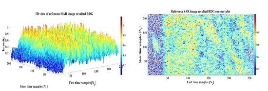
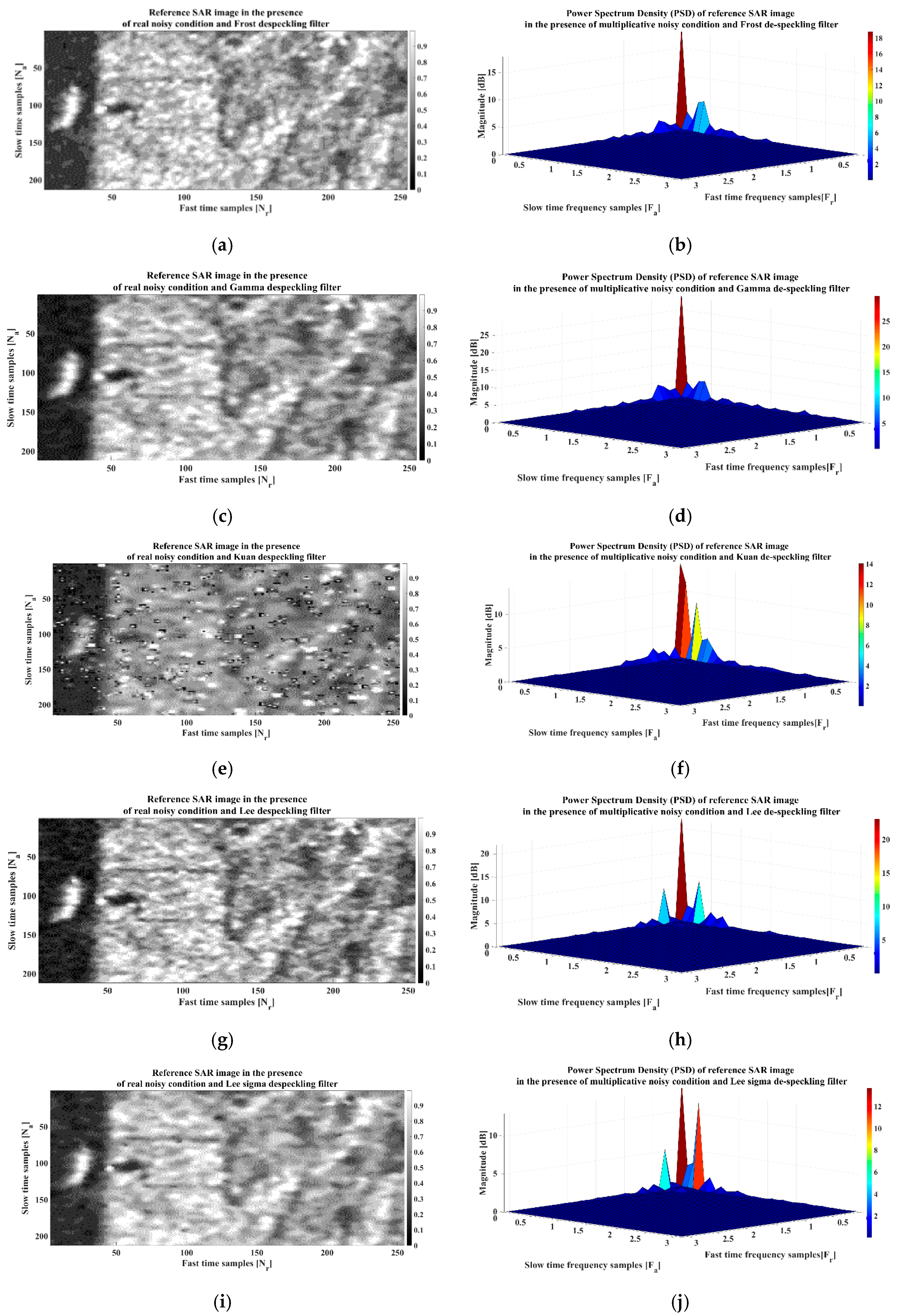
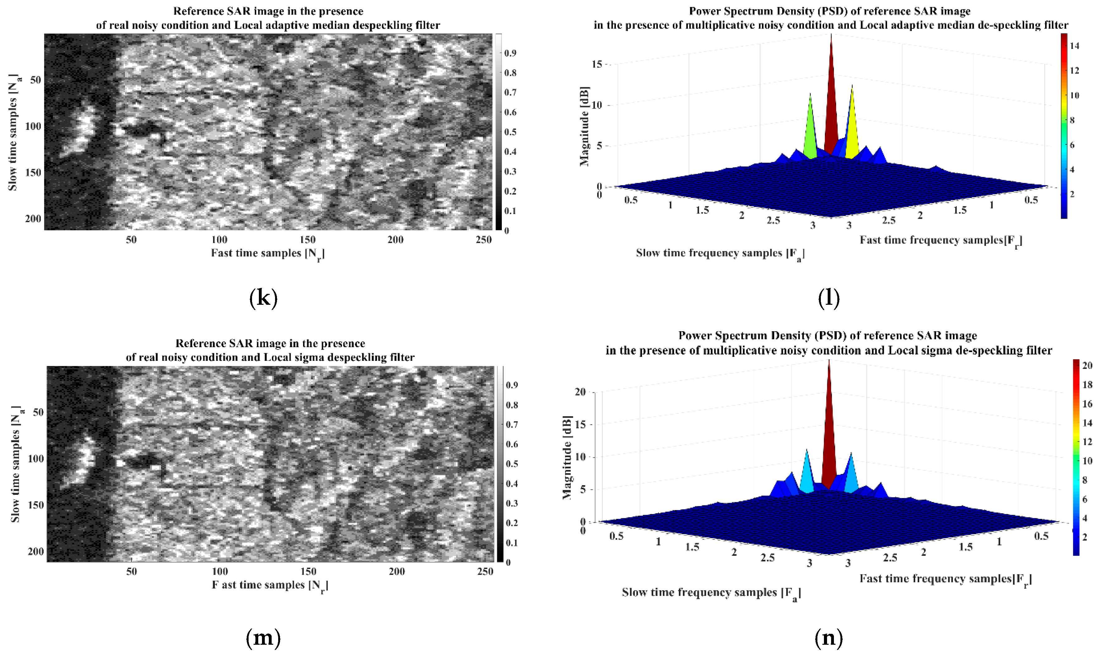
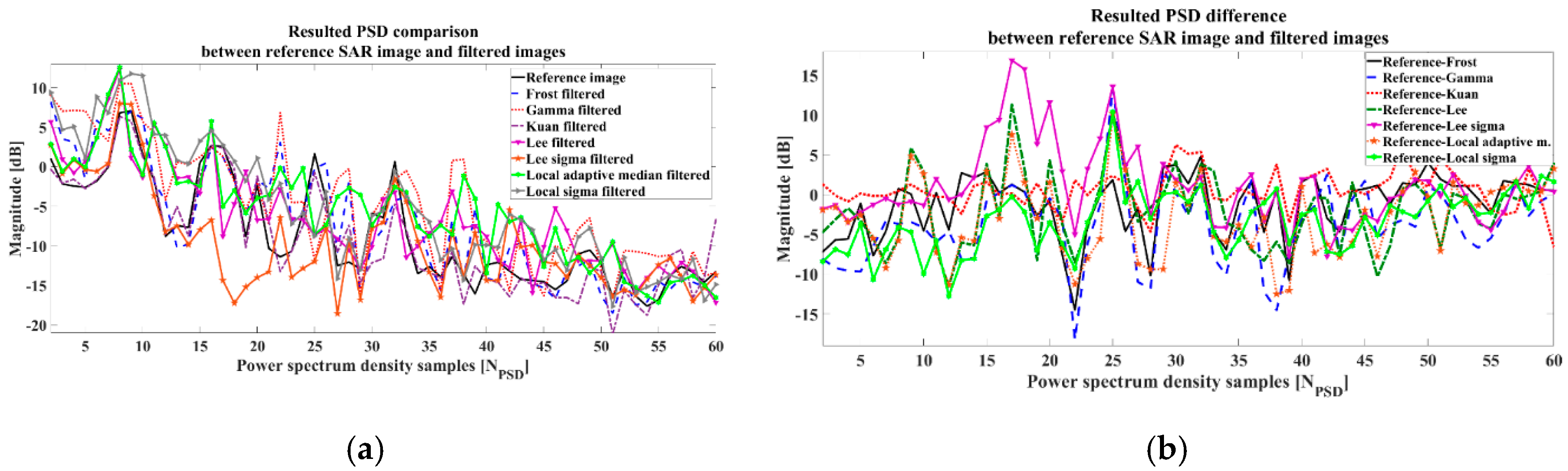
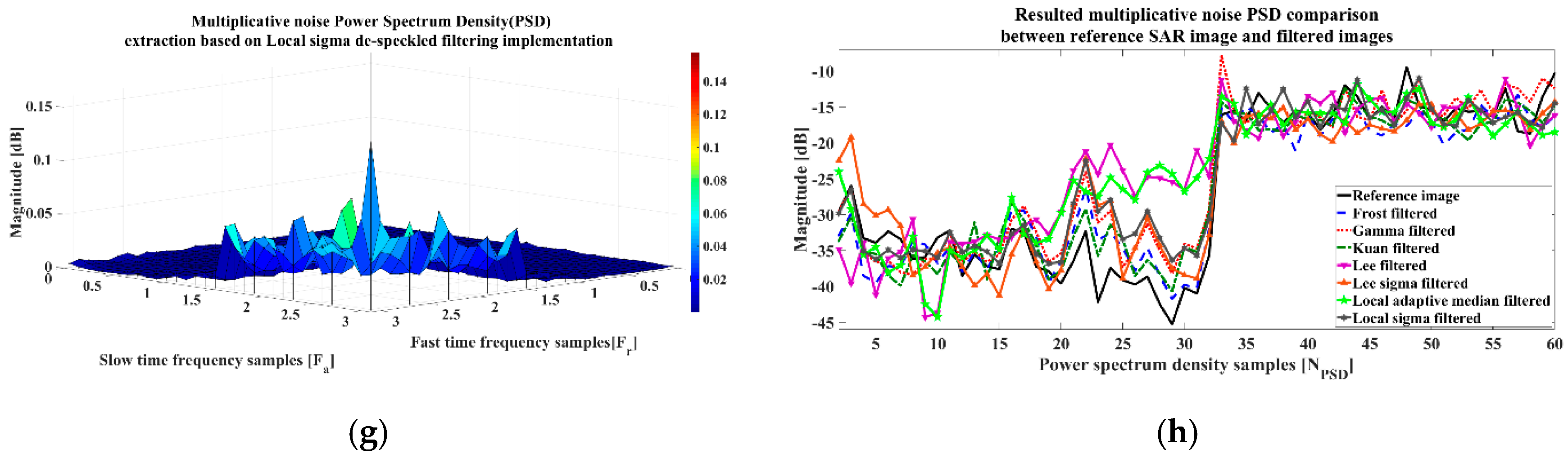
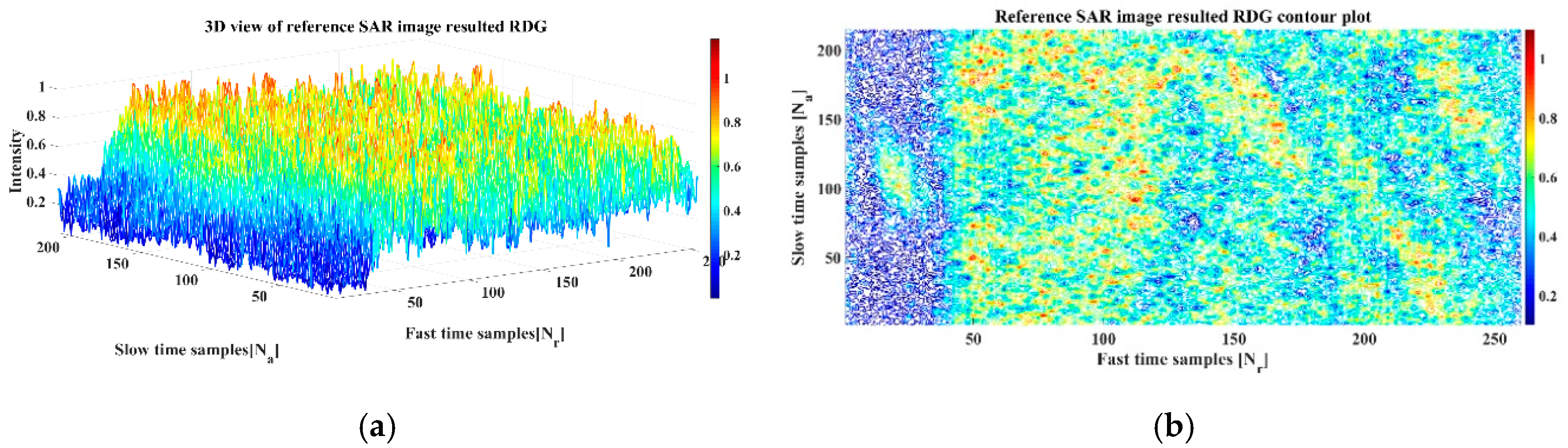
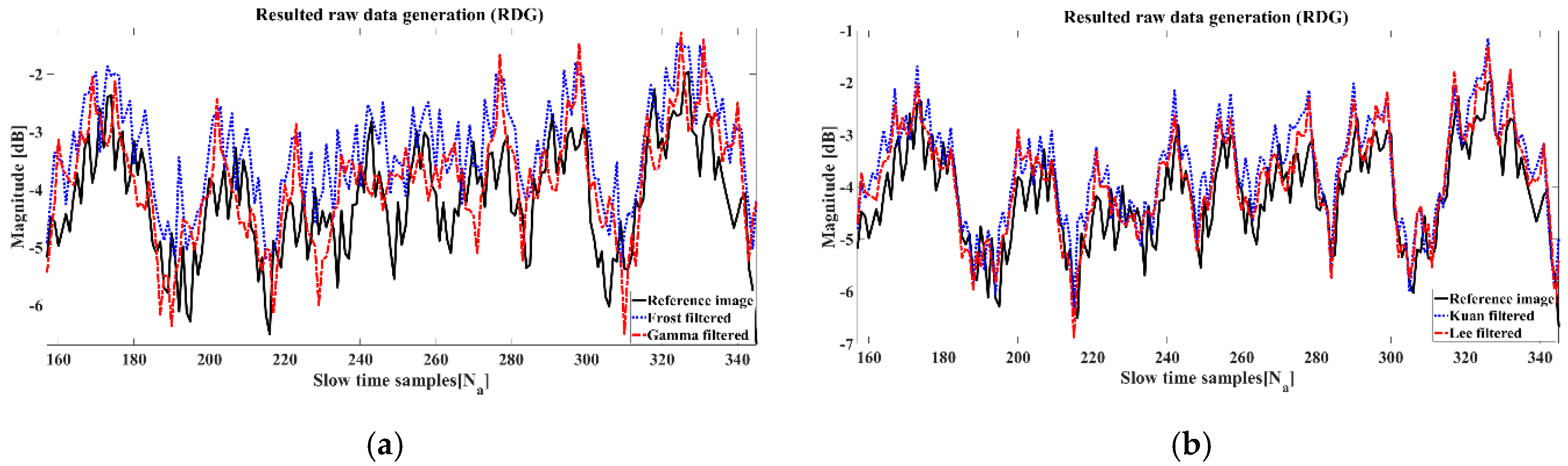
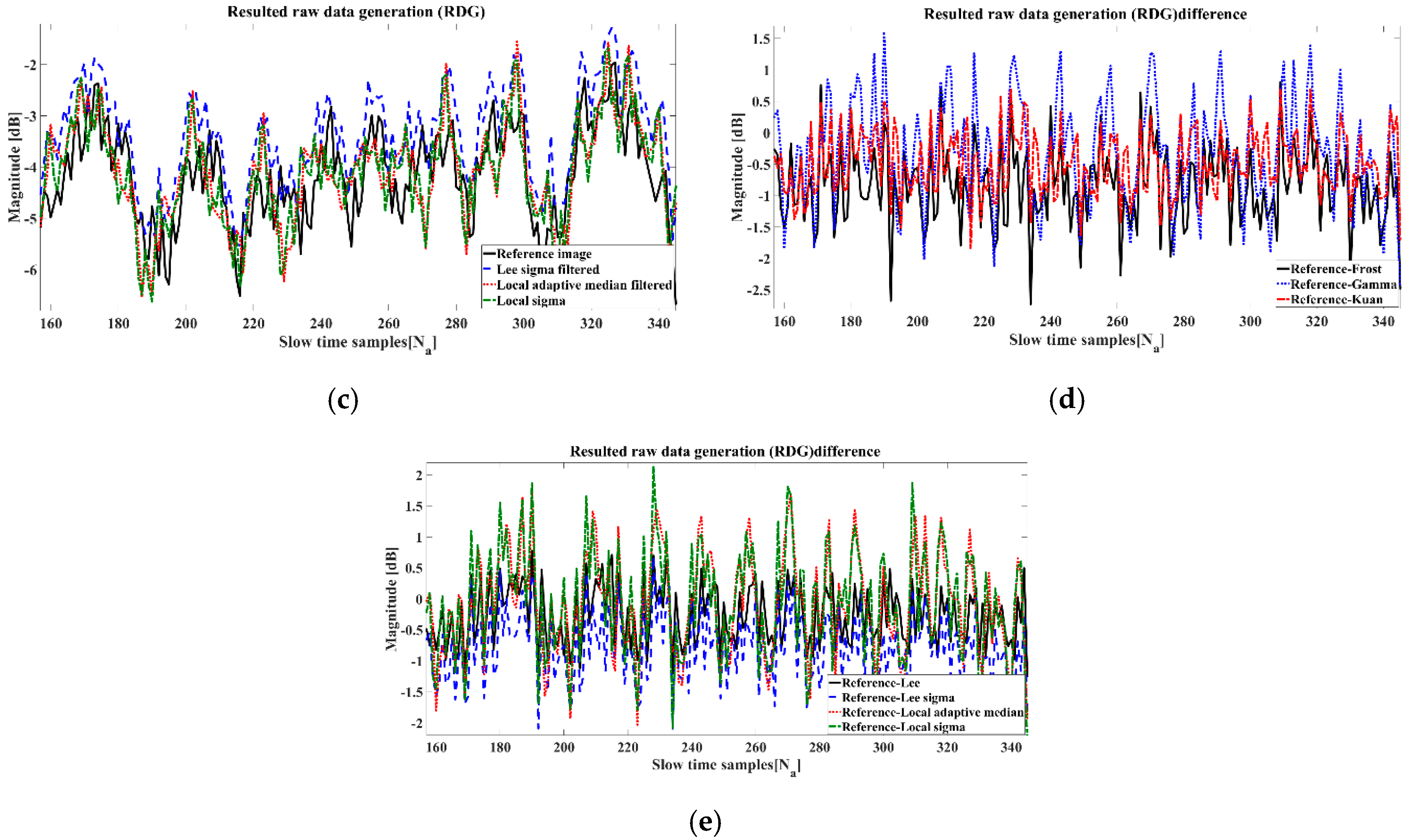
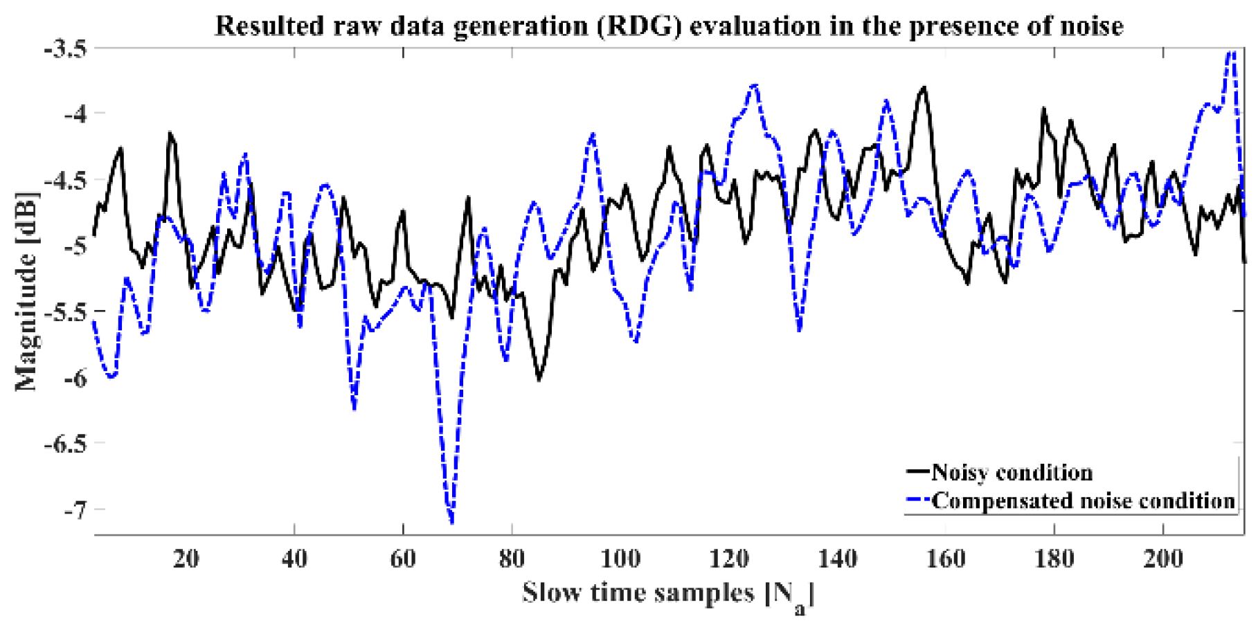
3.1. HMS System Resolution Analysis Based on RDG Extraction

Based on the proposed method, the simulation results of the RDG extraction in the case of the reference SAR image are shown in Figure 7. The results contain a 3-D view of RDG and the contour plot of the reference image. Accordingly, a similar procedure is done on the de-speckled SAR images in Figure 3. All the RDG extraction and comparison results with the reference image are shown in Figure 8. It should be noted that all the RDG simulations were carried out under the system parameters of Table 3. According to Figure 8, the maximum magnitude difference of the RDG between the reference and de-speckled images is about 3.5 dB, which was achieved by the Local sigma filter application. However, in the case of comparison between the other resulting RDGs, the Local sigma, the Local adaptive median, and the Gamma filters have the highest RDG differences with the reference image. As a result, application of the aforementioned spatial de-speckling filters will have destructive effects on the homogeneity of the reconstructed SAR texture. As can be deduced from Figure 8d,e, the high-frequency multiplicative adverse behavior of the HMS while dealing with the raw data is presented as instantaneous changes of the magnitude in the resulting RDG. According to Figure 8, application of a proper spatial de-speckling filter like the Lee sigma with the lowest deviation in the RDG difference obtains the best performance on the phase history of the raw data, which is a sign for better homogeneity of the texture within the reconstructed image. According to Figure 9, in the case of compensated HMS or the noise-free condition, the resulting RDG has less instantaneous changes and it varies smoothly. It also shows that the HMS has really adverse effects on the RDG, which will cause raw data inconsistency. In total, not only does the HMS degrade the system resolution, but also the proper implementation of the spatial de-speckling filter is very important for information retrieval. In other words, the HMS effects on the RDG is presented in the form of instantaneous variations in the magnitude of the RDG or raw data inconsistency. Hence, a complete understanding of the image structure and the texture characteristics for the spatial de-speckling filter application might be helpful for reducing the adverse effects of the HMS on the raw data inconsistency or texture homogeneity.

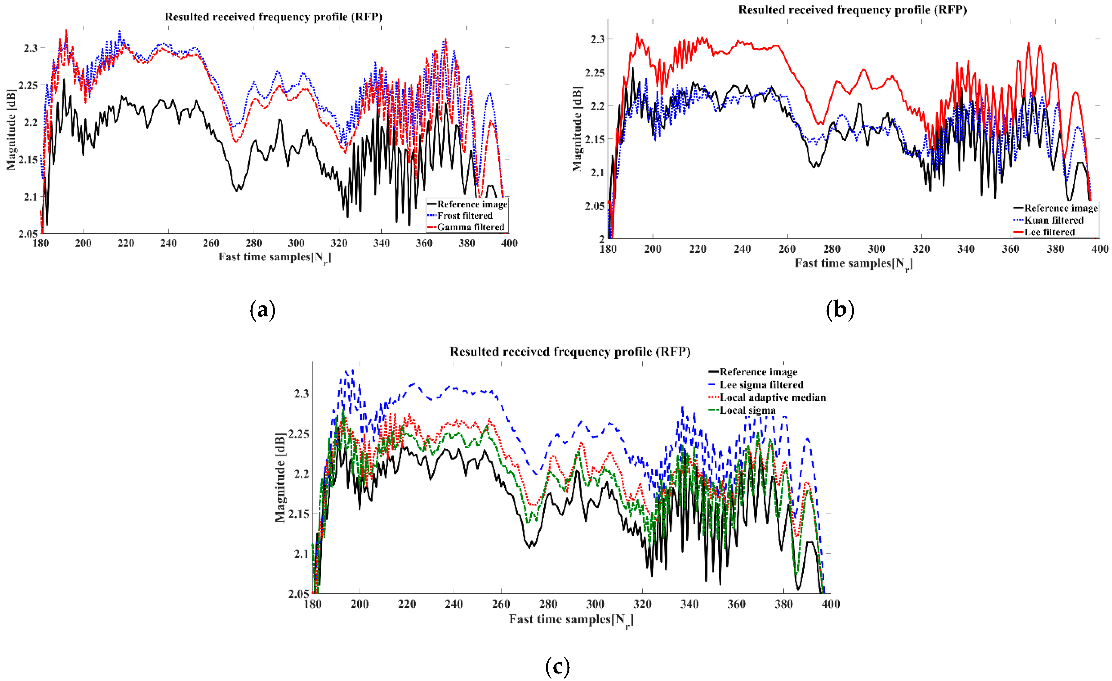
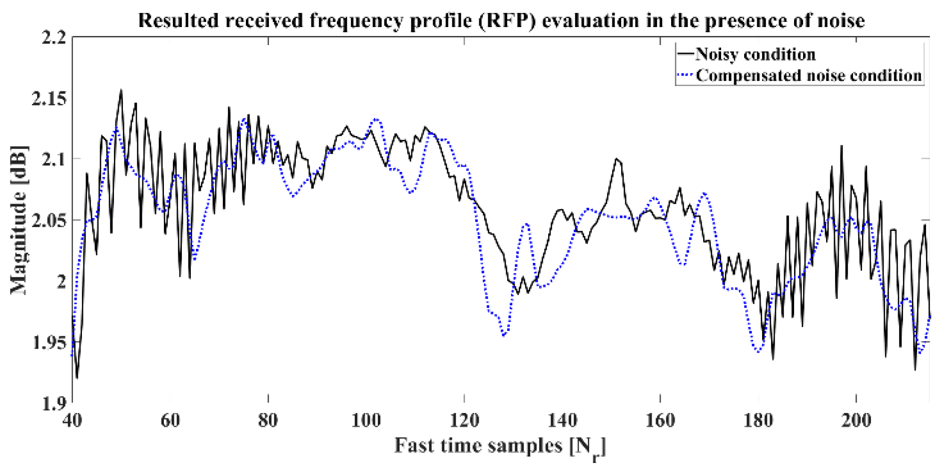
3.2. HMS System Resolution Analysis Based on RFP Extraction

Similar to the RDG extraction, the RFP extraction for the reference SAR image and the de-speckled images were carried out and are presented in Figure 10. According to the results, it can be deduced that the RFP peak-to-peak difference between the reference image and the de-speckled samples are not only the same, but also have few differences in magnitude, with a value of 0.2 dB. In comparison to the RDG simulations and according to Figure 8 and Figure 9, the RFP extraction is more robust to spatial de-speckling filter implementation than the RDG. In other words, the RDG or received 2-D backscattered data is more sensitive to the phase inconsistency and the HMS presence, while the RFP is less sensitive and mostly dependent on the system parameters. This means that radar spatial resolution can be easily affected by high-frequency errors such as geometric and radiometric loss, specifically while dealing with phase coherency, while the RFP as another system resolution criteria is less sensitive to the presence of such errors. Figure 11 also presents the RFP of the reference SAR image in the presence of real noise and noise-free conditions.

As can be seen from Figure 11, HMS also has an effect on the RFP, based on instantaneous changes. However, in comparison to Figure 9, there is less change to the magnitude. In brief, the RFP mainly deals with the system resolution while dealing with the waveform in the receive procedure, but the RDG mainly deals with the waveform while being transmitted and interacting with the CCT. As can be deduced from Figure 7, Figure 8, Figure 9, Figure 10 and Figure 11, the HMS has adverse effects that are more important to the phase history of the backscattered data in comparison to their adverse presence while being processed as part of the signal in the IFA. The results also verify that undertaking CTT studies on aspects such as their complex values, behaviors and specifications in the presence of HMS is difficult, and involves errors that must be considered in comparison to the received signal or image processing.

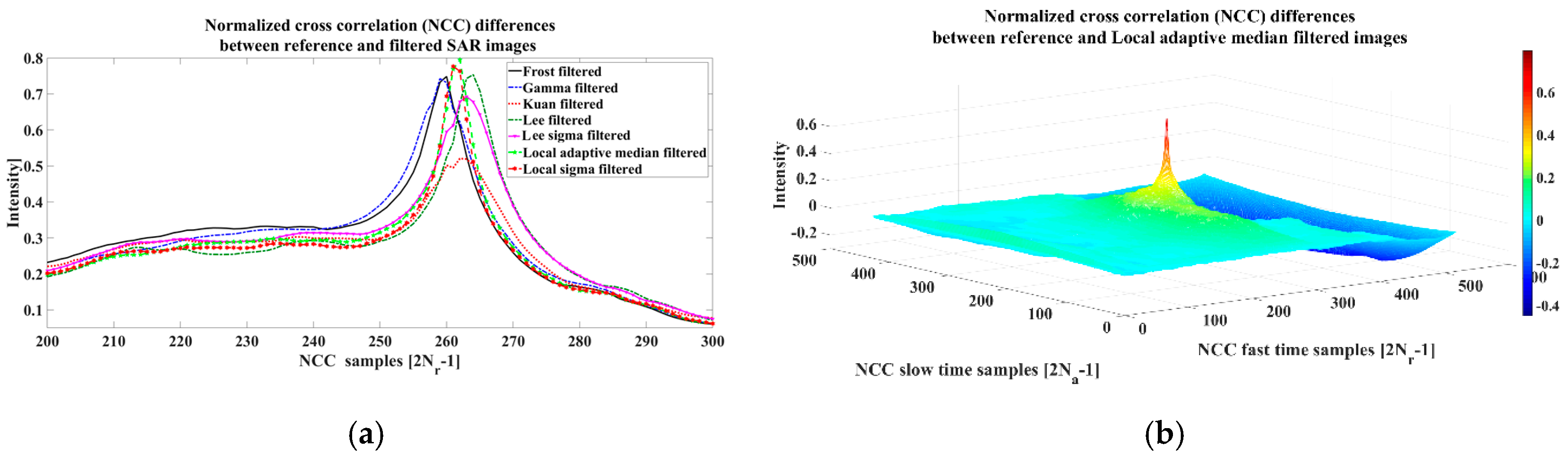
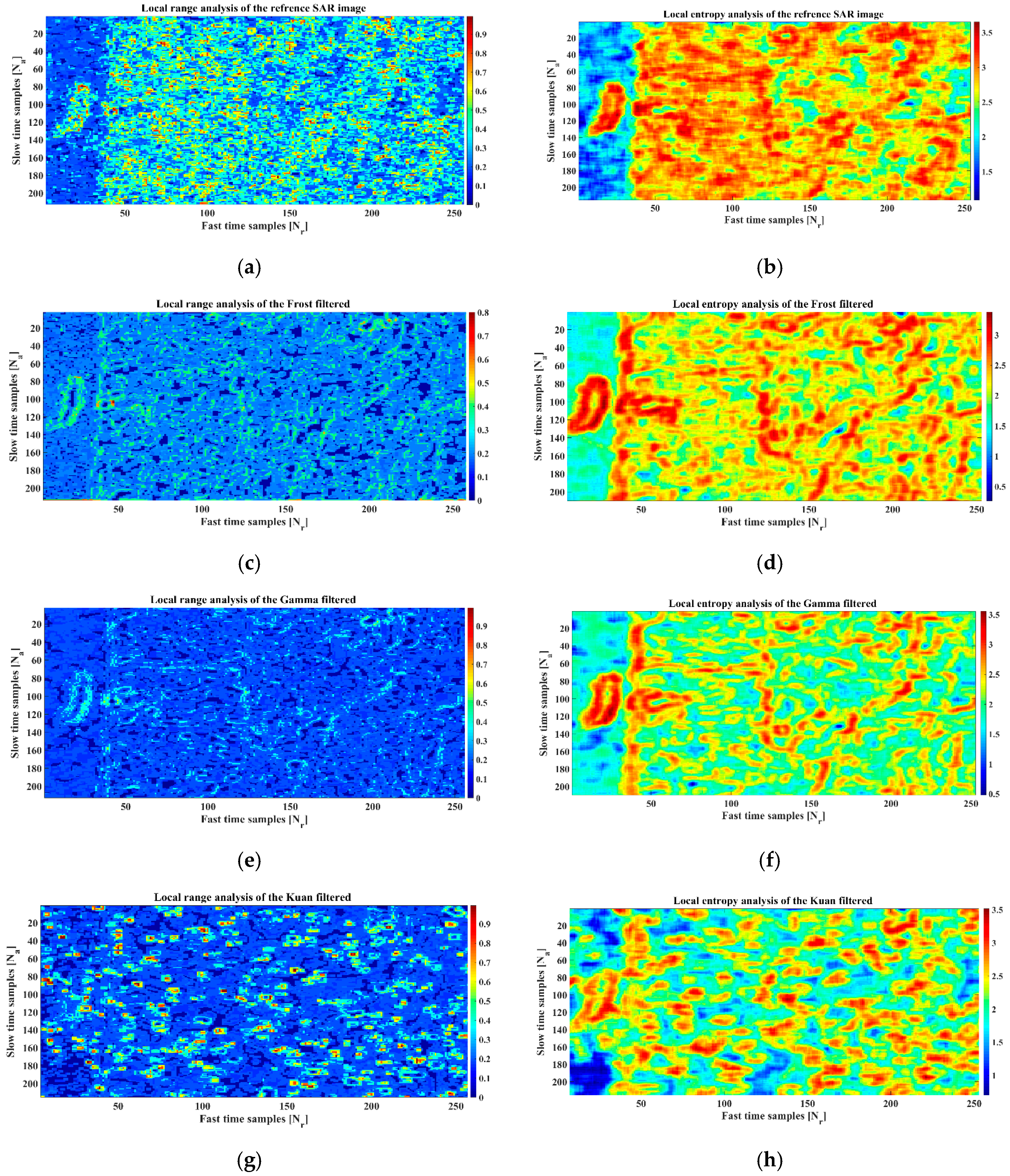
3.3. HMS Image Resolution Analysis Based on Objective Quality Assessment

The implementation of the objective quality assessment technique on the de-speckled SAR images will not only help to evaluate the HMS presence in the SAR images, but also verify the procedure of the spatial de-speckling filter implementation based on image resolution and information analysis. These objective metrics include the mean square error (MSE), the mean intensity value (MIV), the variance (Var), the signal-to-noise ratio (SNR), the peak signal-to-noise ratio (PSNR), the structural similarity index map (SSIM), the mean SSIM (MSSIM), the normalized cross correlation (NCC), the local entropy, and the local range. The MSE, MIV, Var, SNR, PSNR, SSIM and MSSIM are pixel-based measurements, the NCC is correlation-based, and the local entropy and local range are based on image information statistics.

MIV contributes to individual pixel intensity for the entire image, and Var is normally used to find how each pixel varies from the neighboring pixel or the central one. The SNR is the ratio of the mean value of the image and the standard deviation of the HMS within an image. The higher the SNR, the sharper the SAR image will be. The PSNR is the ratio between the maximum possible power of the SAR image and the power of HMS that affects the quality of the image, with the help of MSE as a scaled definition of power by the number of pixels in the images. There is an inverse relationship between PSNR and MSE. Therefore, a higher PSNR value will introduce a lower value of errors. The SSIM index is a quality metric of one of the images being compared to another image, which is regarded as the reference image. The NCC is used as a correlation-based technique to evaluate the degree of similarity between pixel entities of the reference SAR image and the de-speckled images. The local entropy and local range are also 2-D presentations of the images based on pixel and neighboring pixel statistics calculations, which in turn are based on the texture content related to their variations in intensity values or gray levels.

The results of image resolution analysis on the pixel-based quality assessment are listed in

Table 4. SAR images’ pixel-based objective quality metric results.

Image	MSE	MIV	Var.	SNR [dB]	PSNR [dB]	SSIM	MSSIM
Reference	-	0.46	0.05	12.459	-	-	-
Frost	0	0.49	0.05	12.459	-	1	0.9903
Gamma	0	0.49	0.05	12.63	-	1	0.9903
Kuan	0.04	0.50	0.04	13.67	13.60	0.9153	0.9839
Lee	0.04	0.57	0.06	11.94	14.41	0.9506	0.9853
Lee sigma	0.06	0.61	0.05	12.62	12.58	0.9449	0.9825
Local adaptive	0.05	0.51	0.05	12.30	13.44	0.9477	0.9837
Local sigma	0.03	0.49	0.05	12.63	14.61	0.9675	0.9852

. As can be seen from the listed results, every spatial de-speckling filter has its own specification, and in the case of pixel-based image resolution analysis the texture, the image structure, and the parameter of interest play a key role for spatial filter selection. It can also be deduced that Frost and Gamma have the best SSIM values and have great similarity with the reference SAR image, while Kuan and Lee have the lowest values of errors. With the help of correlation-based measurement, the NCC between the reference SAR image and the other de-speckled images is also calculated and presented in Figure 12. Accordingly, the maximum NCC value is related to the Local adaptive median filter with the value of 0.8, while the minimum value is about 0.52, which is related to the Kuan filter. It is clear that in the case of correlation metric evaluation, the Kuan filter, with the best level of pixel-based error measurement, has not achieved the same performance based on correlation index measurements. Figure 12 also presents the NCC of the Local adaptive median filter as having the best performance according to the NCC index.

More detailed texture content processing on the reference SAR image and de-speckled sample images also shows that the HMS has different non-constant effects on the SAR image while being removed with the help of spatial de-speckling filters. The results in Figure 13 attempt to quantify such a non-constant pattern as a function of local entropy and local range presentation. As can be deduced from Figure 13, the results within each de-speckled image are different from each other, and this shows that the SAR image resolution is the most common characteristic to be affected by the HMS and the spatial filter application. The results also prove that an image may only be superior in one metric while being inferior in another in other objective quality metrics. In other words, different spatial de-speckling filters will have different image resolution effects on the textures, and the spatial filter selection is relativistic while dealing with image resolution metrics.

In total, when dealing with the SAR images and de-speckled image quality assessment, system resolution and image resolution are quite different concepts. According to the filter application, such as spectral or resolution and its specific metric, a filter selection must be made. While analyzing the HMS, the RDG is more sensitive to speckle presence in comparison to the RFP. In the case of image resolution assessment, the objective metric is a determinative index for spatial filter selection. The resolutional analysis of the de-speckling procedure will help us to understand the behavior of the HMS and its suitable removal method with less information degradation. In other words, the spatial filter application must be chosen in a way to have the best SAR image information preservation.

4. Discussion

SAR systems are an established technology for remote sensing applications [1]. Owing to the complex recording and processing of the received 2-D backscattered data, SAR sensors are able to form high-resolution complex images of the terrain [3]. The inherent complex nature of SAR data is also one of the main drawbacks of this sensor, as it affects the phase history of the raw data with a specific type of noise known as speckles [4]. Speckles are modeled as multiplicative interference in a destructive or constructive manner in the SAR phase history, and its suppression or de-speckling has been always a major challenge in SAR image processing [5]. In general, speckle reduction techniques are applied prior to texture feature extraction, and the de-speckling has been considered as an active field of research in remote sensing processing [8]. However, the main problem of SAR image de-speckling is resolution preservation, because both the speckle presence and de-speckling procedure degrade the quality of the image and might lead to misinterpretation [21]. These considerations motivate the increasingly intense research for speckle analysis and precise de-speckling methods with the help of spatial de-speckling filters, without impairing potentially valuable SAR image information [19]. Considering the complexity of spatial de-speckling filter implementation, it is necessary to perform an objective quality analysis on the embedded multiplicative noise within the SAR images for the purpose of speckle behavioral analysis and proper filter selection.

To retrieve such objective metrics, this paper considers a reference SAR image under seven different spatial de-speckling filter implementations for the purpose of speckle presence analysis and filtering evaluation. This is the first time that this type of evaluation scenario has been categorized into three major procedures. The evaluation scenario not only covers the spectral simulation of the speckle on the basis of the image and the noise, but also covers the objective quality assessment in the case of system resolution and image resolution analysis. The spectral simulation includes the PSD function formulation and modeling, while the system resolution and the image resolution contain the RDG, RFP, pixel-based, correlation-based, local entropy, and local range measurements. All the resulting qualitative and quantitative metrics verify that not only are the multiplicative speckle-noise presented in the high-frequency part of the image information with no specific pattern within the texture, but also that no spatial de-speckling filter consistently outperforms the others in suppression. In other words, the novel results of this research analysis show that every specific aforementioned category, such as spectral modeling, system resolution and image resolution, has its own filter or filters with the best and the worst performance.

Hence, in the case of the aforementioned spatial de-speckling filters, the results are listed as follows: (i) According to the spectral modeling of the spatial filters, Gamma has the best and Lee sigma has the worst de-speckling performance. (ii) For the purpose of residue speckle measurement, Local sigma has the best performance, while Gamma has the worst ability to measure the level of the remaining noise presence. (iii) According to system resolution measurement based on the RDG index, Lee has the best system performance while Local sigma has the worst evaluation, and Kuan has the best performance in comparison to Lee sigma if the RFP is going to be considered. (iiii) Finally, in the case of the image resolution analysis, the spatial filter selection is completely relativistic and dependent on criteria such as pixel-based, correlation based, local entropy, or range line results. This research study not only verifies that multiplicative speckle noise is located within the high-frequency part of the image information with no specific pattern within the texture, but also the proposed spatial de-speckling filter for the proper application. The results also help to categorize spatial de-speckling filters as spectral filters, system resolution enhancement filters, and image resolution improvement applications, while their objective image quality metrics play an important role for their selection and implementation. Future studies might include other types of de-speckling filters, such as transform domain filters with more objective quality metric verifications based on time-domain, frequency-domain and time-frequency domain analysis, however the texture and the application purpose remain very important.

5. Conclusions

SAR images are inherently degraded by the phase interferences of received 2-D backscattered signals, which results in a high-frequency multiplicative noise known as speckle. Speckle reduction methods are applied before texture information extraction with the help of spatial de-speckling filters. Since the performance of speckle noise suppression must be consistent with the application of de-speckling filters in order to preserve fine details and subtle textures, a novel speckle analysis method, as well as de-speckling filter categorization and evaluation, have been proposed in this research study. The categorization resulted in three major groups of spatial filters: spectral filters, system resolution enhancement filters, and image resolution improvement filters. This research study also introduces spatial de-speckling filter implementation results based on their performance in the best- and the worst-case applications, according to their categories. The results of this research study can also be used as an evaluation protocol for spatial filter performance and speckle removal evaluation. The sample filters in this study are Frost, Kuan, Gamma, Lee, Lee sigma, Local adaptive median, and Local sigma, and all the simulation results were derived based on the spectral analysis, the system resolution, and the image resolution criteria. The results clearly show that selecting a proper spatial de-speckling filter for the best noise suppression is completely dependent on the category of interest. However, the superiority of the performance is dependent on the quality objective metric comparison.

References

1. Barnes, C.F. Synthetic Aperture Radar: Wave Theory Foundations, Analysis and Algorithms; Barnes: Powder Spring, GA, USA, 2015. [Google Scholar]
2. Chen, K.S. Principles of Synthetic Aperture Radar Imaging; Taylor & Francis Group: Boca Raton, London, UK, 2016. [Google Scholar]
3. Cumming, I.G.; Wong, F.H. Digital Processing of Synthetic Aperture Radar Data; Artech House: Boston, MA, USA, 2005. [Google Scholar]
4. Argentini, F.; Lapini, A.; Bianchi, T.; Alparone, L.A. Tutorial on speckle reduction in synthetic aperture radar. IEEE Trans. Geosci. Remote Sens. 2013, 1, 6–35. [Google Scholar] [CrossRef]
5. Liu, F.; Wu, J.; Li, L.; Jiao, L.; Hao, H.; Zhang, X. A hybrid method of SAR speckle reduction based on geometric-structural block and adaptive neighborhood. IEEE Trans. Geosci. Remote Sens. 2018, 56, 730–748. [Google Scholar] [CrossRef]
6. Yahya, N.; Kamel, N.S.; Malik, A.S. Subspace-based technique for speckle noise reduction in SAR images. IEEE Trans. Geosci. Remote Sens. 2014, 52, 6257–6271. [Google Scholar] [CrossRef]
7. Di Martino, G.; Simone, A.D.; Lodice, A.; Ricco, D. Scattering-Based nonlocal means SAR despeckling. IEEE Trans. Geosci. Remote Sens. 2016, 54, 3574–3588. [Google Scholar] [CrossRef]
8. Gleich, D. Optimal-Dual-Based l1 Analysis for Speckle Reduction of SAR Data. IEEE Trans. Geosci. Remote Sens. 2018, 56, 6674–6685. [Google Scholar] [CrossRef]
9. Di Martino, G.; Lodice, A.; Riccio, D.; Ruello, G. Equivalent number of scatterers for SAR speckle modeling. IEEE Trans. Geosci. Remote Sens. 2014, 52, 2255–2564. [Google Scholar] [CrossRef]
10. Zhao, W.; Deledalle, C.A.; Denis, L.; Maître, H.; Nicolas, J.M.; Tupin, F. Ratio-based multitemporal SAR images denoising: RABASAR. IEEE Trans. Geosci. Remote Sens. 2019, 1–14. [Google Scholar] [CrossRef]
11. Frost, V.S.; Stiles, J.A.; Shunmugan, K.S.; Holtzman, J.C. A Model for Radar Images and Its Application to Adaptive Digital Filtering of Multiplicative Noise. IEEE Trans. Pattern Anal. Mach. Intell. 1982, 4, 157–166. [Google Scholar] [CrossRef]
12. Lee, J.S. A Simple Speckle Smoothing Algorithm for Synthetic Aperture Radar Images. IEEE Trans. Syst. Man Cybern. 1983, 13, 85–89. [Google Scholar] [CrossRef]
13. Kuan, D.; Sawchuk, A.; Strand, T.; Chavel, P. Adaptive Restoration of Images with Speckle. IEEE Trans. Acoust. Speech Signal Process. 1987, 35, 373–383. [Google Scholar] [CrossRef]
14. Touzi, R. A review of speckle filtering in context of estimation theory. IEEE Trans. Geosci. Remote Sens. 2002, 40, 2392–2404. [Google Scholar] [CrossRef]
15. Goodman, J.W. Speckle phenomenon in optics: Theory and applications. J. Stat. Phys. 2008, 130, 413–414. [Google Scholar]
16. Amirmazlaghani, M.; Amindavar, H. A novel sparse method for despeckling SAR images. IEEE Trans. Geosci. Remote Sens. 2012, 50, 5024–5032. [Google Scholar] [CrossRef]
17. Di Martino, G.; Poderico, M.; Poggi, G.; Riccio, D.; Verdoliva, L. Benchmarking Framework for SAR Despeckling. IEEE Trans. Geosci. Remote Sens. 2014, 52, 1596–1615. [Google Scholar] [CrossRef]
18. Deledalle, C.A.; Denis, L.; Poggi, G.; Tupin, F.; Verdoliva, L. Exploiting patch similarity for SAR image processing: The nonlocal paradigm. IEEE Signal Process. Mag. 2014, 31, 69–78. [Google Scholar] [CrossRef]
19. Lang, F.; Yang, J.; Li, D. Adaptive-Window polarimetric SAR image speckle filtering based on a homogeneity measurement. IEEE Trans. Geosci. Remote Sens. 2015, 53, 5435–5446. [Google Scholar] [CrossRef]
20. Zhao, Y.; Liu, J.G.; Zhang, B.; Hong, W.; Wu, Y. Adaptive total variation regularization based SAR image despeckling and despeckling evaluation index. IEEE Trans. Geosci. Remote Sens. 2015, 53, 2765–2774. [Google Scholar] [CrossRef]
21. Wang, Y.; Ainsworth, T.L.; Lee, J.S. Application of mixture regression for improved polarimetric SAR speckle filtering. IEEE Trans. Geosci. Remote Sens. 2017, 55, 453–467. [Google Scholar] [CrossRef]
22. Ozcan, C.; Sen, B.; Nar, F. Sparisity-driven despeckling for SAR images. IEEE Geosci. Remote Sens. Lett. 2016, 13, 115–119. [Google Scholar] [CrossRef]
23. Ma, X.; Wu, P.; Shen, H. A nonlinear guided filter for polarimetric SAR image despeckling. IEEE Trans. Geosci. Remote Sens. 2019, 57, 1918–1927. [Google Scholar] [CrossRef]
24. Liu, Y.; Wang, W.; Pan, X.; Gu, Z.; Wang, G. Raw signal simulator for SAR with trajectory deviation based on spatial spectrum analysis. IEEE Trans. Geosci. Remote Sens. 2017, 55, 6651–6665. [Google Scholar] [CrossRef]
25. Ni, W.; Gao, X. Despeckling of SAR image using generalized guided filter with Bayesian nonlocal means. IEEE Trans. Geosci. Remote Sens. 2016, 54, 567–579. [Google Scholar] [CrossRef]
Figure 1. Geometry of the illumination from the antenna toward the CTT.
Remotesensing 11 01041 g001
Figure 2. Reference SAR image and its PSD modeling (a) Reference SAR image; (b) PSD of reference SAR image; (c) PSD of reference SAR image in presence of little noise; (d) PSD of reference SAR image in noise-free medium; (e) PSD of high-frequency noise.
Remotesensing 11 01041 g002
Figure 3. SAR images with different de-speckled filters and their relative PSD modeling (a) Frost; (b) Frost PSD; (c) Gamma; (d) Gamma PSD; (e) Kuan; (f) Kuan PSD; (g) Lee; (h) Lee PSD; (i) Lee sigma; (j) Lee sigma PSD; (k) Local adaptive median; (l) Local adaptive median PSD; (m) Local sigma; (n) Local sigma PSD.
Remotesensing 11 01041 g003aRemotesensing 11 01041 g003b
Figure 4. Resulting PSD modeling (a) comparison (b) difference with the reference SAR image.
Remotesensing 11 01041 g004
Figure 5. PSD of the residue HMS after the de-speckling procedure (a) Frost; (b) Gamma; (c) Kuan; (d) Lee; (e) Lee sigma; (f) Local adaptive median; (g) Local sigma; (h) Comparison of the residue HMS.
Remotesensing 11 01041 g005aRemotesensing 11 01041 g005b
Figure 6. Proposed system resolution extraction algorithm with the help of range cell migration cancellation (RCMC).
Remotesensing 11 01041 g006
Figure 7. Resulting RDG of the reference image (a) RDG 3-D plot; (b) RDG contour plot.
Remotesensing 11 01041 g007
Figure 8. Resulting RDG presentation (a) Reference, Frost and Gamma (b) Kuan, Lee (c) Lee sigma, Local adaptive median and Local sigma—resulting RDG differences (d) Frost, Gamma and Kuan (e) Lee, Lee sigma, Local adaptive median and Local sigma—RDG evaluation.
Remotesensing 11 01041 g008aRemotesensing 11 01041 g008b
Figure 9. Reference RDG evaluation in the presence of noise and compensated noise conditions.
Remotesensing 11 01041 g009
Figure 10. Resulting RFP presentation (ac).
Remotesensing 11 01041 g010
Figure 11. Reference RFP evaluation in the presence of noise and compensated noise conditions.
Remotesensing 11 01041 g011
Figure 12. NCC (a) difference between the reference SAR image and de-speckled sample; (b) between the Local adaptive median filter and reference image.
Remotesensing 11 01041 g012
Figure 13. Texture content analysis based on local range and local entropy (a) reference SAR image; (b) reference SAR image; (c) Frost filtered; (d) Frost filtered; (e) Gamma filtered; (f) Gamma filtered; (g) Kuan filtered; (h) Kuan filtered; (i) Lee filtered; (j) Lee filtered; (k) Lee sigma filtered; (l) Lee sigma filtered; (m) Local adaptive median filtered; (n) Local adaptive median filtered; (o) Local sigma; (p) Local sigma.
Remotesensing 11 01041 g013aRemotesensing 11 01041 g013b