Distribution and Morphologies of Transverse Aeolian Ridges in ExoMars 2020 Rover Landing Site


1
Division of Space Technology, Department of Computer Science, Electrical and Space Engineering, Luleå University of Technology, 97187 Luleå, Sweden
2
Instituto Andaluz de Ciencias de la Tierra (CSIC-UGR), Armilla, 18100 Granada, Spain
3
Centro de Astrobiología (INTA-CSIC), Torrejón de Ardoz, 28850 Madrid, Spain
*
Author to whom correspondence should be addressed.
Remote Sens. 2019, 11(8), 912; https://doi.org/10.3390/rs11080912
Submission received: 5 March 2019
/
Revised: 12 April 2019
/
Accepted: 12 April 2019
/
Published: 15 April 2019
(This article belongs to the Special Issue Remote Sensing in Support of Aeolian Research)
Abstract
:Aeolian processes are believed to play a major role in the landscape evolution of Mars. Investigations on Martian aeolian landforms such as ripples, transverse aeolian ridges (TARs), and dunes, and aeolian sediment flux measurements are important to enhance our understanding of past and present wind regimes, the ongoing dust cycle, landscape evolution, and geochemistry. These aeolian bedforms are often comprised of loose sand and sharply undulating topography and thus pose a threat to mobility and maneuvers of Mars rovers. Here we present a first-hand account of the distribution, morphologies, and morphometrics of TARs in Oxia Planum, the recently selected ExoMars 2020 Rover landing site. The gridded mapping was performed for contiguous stretches of TARs within all the landing ellipses using 57 sub-meter high resolution imaging science experiment (HiRISE) scenes. We also provide the morphological descriptions for all types of TARs present within the landing ellipses. We use HiRISE digital terrain models (DTMs) along with the images to derive morphometric information for TARs in Oxia Planum. In general, the average areal TAR coverage was found to be 5.4% (±4.9% standard deviation), increasing from west to east within the landing ellipses. We report the average TAR morphometrics in the form of crest–ridge width (131.1 ± 106.2 m), down-wind TAR length (17.6 ± 10.1 m), wavelength (37.3 ± 11.6 m), plan view aspect ratio (7.1 ± 2.3), inter-bedform spacing (2.1 ± 1.1), slope (10.6° ± 6.1°), predominant orientations (NE-SW and E-W), and height (1.2 ± 0.8 m). While simple TARs are predominant, we report other TAR morphologies such as forked TAR, wavy TAR with associated smaller secondary ripples, barchan-like TAR, networked TAR, and mini-TARs from the region. Our results can help in planning the rover traverses in terms of both safe passage and scientific returns favoring aeolian research, particularly improving our understanding of TARs.
1. Introduction
Aeolian processes have played a significant role in landscape evolution and development of surficial features on planets with considerable atmospheres such as Earth, Mars, and Venus [1]. For Mars, the substantial influx of orbiter, lander, and rover imagery and geophysical data with continuously improving resolutions in the past two decades have largely facilitated our understanding of the relict and active aeolian processes and landforms, proving aeolian processes to be one of the dominant surface-modifying agents on Mars [2]. Initially the coarser resolution images of Mariner 9 [3] and Viking Orbiters [4] during the 1970s revealed large, low albedo dune masses or large dark dunes (LDDs). The advent of higher-resolution remote sensors, such as the Mars Orbiter Camera (MOC) [5], High Resolution Stereo Camera [6], Context (CTX) Camera [7], and the high resolution imaging science experiment (HiRISE) [8], during the 1990s and 2000s have significantly aided Mars research [9] and made it possible to better study smaller aeolian landforms such as wind ripples, granule ripples, dust devils, yardangs, ventifacts, and transverse aeolian ridges (TARs). Even though the atmosphere of Mars is considerably thinner (i.e., ~1% of Earth’s), the abundance of such landforms on Mars demonstrates strong atmosphere–lithosphere coupling over a large spatiotemporal domain [10]. Thus, these aeolian features and underlying interactions can tell us more about the climate and landscape evolutions on Mars and their presence highlights the regions with past or ongoing sediment transport [11]. In a majority of the cases, we are largely uncertain about the sediment volumes, their origin and traverse, extent, and their composition [11]. Due to the combination of these unknowns and the improvement in data resolutions and simulations, Mars aeolian research has been gaining momentum in the recent years. Several papers [12,13,14,15] over the past decades have reported on manual or semi-automated mapping of features like ripples and sand dunes on Mars at global and regional scales to help our understanding.
TARs are one of the predominant aeolian landforms found in all kinds of geologic settings in equatorial and mid-latitudes (mostly between +35° and −55°) [11,16] on Mars. TARs have decameter-scale wavelengths, intermediate between the small centimeter-scale wind ripples and the large kilometer-scale dunes [17]. TARs were first named by Bourke et al. [18] and the precise information on their origin and sediment source, formation mechanisms, composition, distribution, activity, age, and superposition relationships are yet to be confirmed [19]. However, several interpretations [2,20] envisage them as granule ripples under a surface layer of mm-sized particles, too coarse to be moved by the present-day Martian winds [17]. There are several reported possible terrestrial analogs for Martian TARs, such as the megaripples in Argentina [21] and in the Lut Desert of Iran [19,22], megaripples at Wau-an-Namus, Libya [23], and reversing sand dunes in Idaho, USA [24]. TARs have generally brighter or similar albedo as the surrounding terrain and can occur singularly or as large contiguous stretches [10,22]. The albedo of bright TARs is as high as >0.21, nearly double the albedo of dark dunes [10]. They normally display simple, forked, sinuous, networked, and barchan-like patterns [10]. TARs are landforms with symmetric cross-sectional profiles normally displaying slopes of <28° and maximum height-to-wavelength ratios of ~0.13–0.17 [17,20]. However, in a recent global survey of their morphologies, TARs have been reported to display widely varying morphologies and uncorrelated distribution with latitudes and altitudes [17]. This survey [17] reports average TAR heights to be 2.6 m with a standard deviation of 1.4 m, while the tallest reported TAR reached a maximum height of 14 m. Another independent survey [25] reports typical dimensions of 88.5 m, 17.3 m, 1.3 m, and 25.8 m for length, width, height, and wavelength, respectively, of the mapped TARs. Geissler and Wilgus [17] further reported height-to-wavelength ratios to be weakly anti-correlated with TAR wavelengths, and no correlation between wavelengths and the local slope. Usually TARs in a region display similar orientations over large areas indicating their adaptation to the large-scale wind patterns irrespective of the local topography [26]. Granular megaripples are often considered as a terrestrial analog for TARs.
Oxia Planum, the selected ExoMars 2020 Rover landing site (Figure 1 and Figure 2), was preferred over Mawrth Vallis [27] in the final ExoMars 2020 site selection meeting of European scientists and engineers held at the UK’s National Space Centre in Leicester on 8 and 9 November 2018 due to the greater safety margins that the terrain in Oxia Planum offers for a successful landing and the rover’s mobility. For ensuring the best scientific returns from the planned ExoMars mission, it is necessary to scrutinize the terrain and landforms in Oxia Planum at high resolutions to better guide future traverses and mobility of the rover from the point of landing. As explained above, aeolian landforms, particularly TARs, are not only interesting science targets [28], but they also pose a threat to landing and rover mobility [29] in terms of sand/dust depositions, direct physical damage to the lander or rover chassis and wheels, sinkage into the loose unconsolidated aeolian material [30,31], enhanced slippage [30,32], and permanent entrapment [33]. Sullivan et al. [28,29] provide detailed experimental background of Mars Exploration Rover (MER) Opportunity and MER Spirit where these rovers encountered TARs repeatedly in Meridiani Planum and Gusev Crater, respectively, because TARs were unavoidable during several traverse segments; but the scientific teams wisely used this as an opportunity to closely investigate TARs and other aeolian features. Similarly, the Mars Science Laboratory (MSL) Curiosity Rover during sols 526–538 of its operation at Dingo Gap Bedform in Gale Crater encountered a large 1 m-high megaripple and photographic, as well as spectroscopic cameras, onboard the rover were simultaneously used to study an intended wheel scuff [29]. The ExoMars 2020 Lander and Rover are also equipped with several instruments of this kind which can provide in-situ information to validate remote observations and help our understanding of TARs. For example, the lander has meteorological instruments such as HabitAbility: Brine Irradiation and Temperature (HABIT) and the meteorological package to provide meteorological context of the visual, spectroscopic, and radar observations made by the rover instruments, such as the Panoramic Camera (PanCam), Infrared Spectrometer for ExoMars (ISEM), Close-UP Imager (CLUPI), Water Ice and Subsurface Deposit Observation on Mars (WISDOM), Mars Multispectral Imager for Subsurface Studies (Ma_MISS), the visible and infrared imaging spectrometer MicrOmega, and the Raman spectrometer (RLS). In addition, the ExoMars 2020 is equipped with a drill that embeds Ma_MISS and can reach the subsurface to a maximum depth of 2 m. These instruments make the ExoMars 2020 rover an ideal platform to conduct aeolian research and promote a region-wide high-resolution mapping of TARs and other aeolian landforms. Thus, in the present study, we aim to map all the expected landing ellipses (3-σ) [34] covering a total area of 3211.07 km2 in the Oxia Planum region for TARs (Figure 2). We start with three main objectives to present an account of region-wide (1) distribution, (2) morphologies, and (3) morphometries of TARs in Oxia Planum. We first provide a brief introduction of Oxia Planum as the study site, followed by the methods used to reach the above-mentioned objectives. Our results can help plan the rover traverses in terms of both safe passage and scientific returns favoring aeolian research, particularly improving our understanding of TARs. Similar studies should be applied in the future to other potential regions of interest for landing missions on Mars, as TARs are not only relevant for mobility, but also for the safety assessment of the Entry, Descent, and Landing (EDL) phase.
2. Study Area
The Oxia Planum landing site (16° to 19°N, 337 to 332°W) is located at the edge of an ancient basin called Chryse Planitia and is characterized by ~4 billion-year-old sedimentary clay deposits. This region is marked by ancient highland cratered terrains highly eroded towards the highland–lowland boundary and falls in a wide basin at the outlet of the Cogoon Vallis System between Mawrth Vallis and Ares Vallis [35]. The geomorphological setting of the region and the composition of clay deposits indicate a possibility of them being lagoon or deltaic deposits near an ancient Martian ocean [35]. These layered exposures in the Oxia Planum region are rich in iron and magnesium phyllosilicates and possibly represent the south-western extension of the clay-rich Mawrth Vallis deposits [35].
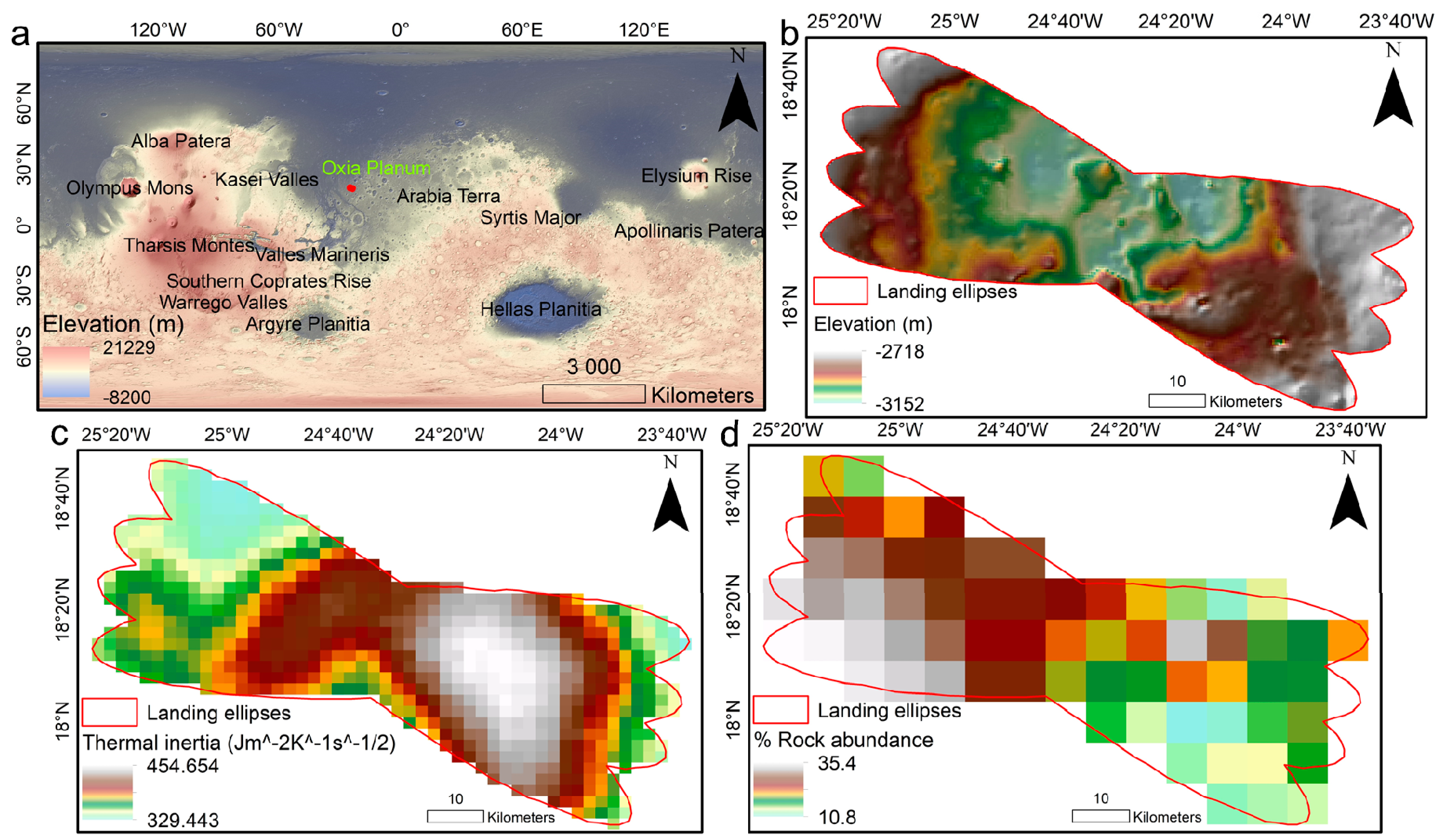
For all the mapping and derived inferences within our study, the study area henceforth will refer to the region shown in Figure 1a–c (i.e., within the expected 3-σ boundaries of the landing ellipses as mentioned by Bridges et al. [34]), with an areal coverage of 3211.07 km2. The elevation range of the study area as derived from Mars Orbiter Laser Altimeter (MOLA) topography is between −2718 and −3152 m (Figure 1b) with a mean elevation of −3031.45 m and standard deviation of 72.86 m. The lowest elevations in the middle of the study area are quite evident (Figure 1b). When we plotted the Mars Global Surveyor (MGS) Thermal Emission Spectrometer (TES)-derived thermal inertia (TI) data [36] at 2 km/pixel resolution, the minimum and maximum TI values were 329.44 Jm−2K−1s−1/2 and 454.65 Jm−2K−1s−1/2, respectively, with a mean TI of 395.52 Jm−2K−1s−1/2 and a standard deviation of 30.4 Jm−2K−1s−1/2. The TI was found to be generally increasing from west-to-east (Figure 1c) within the study area. We further analyzed TES-derived rock abundance [37] data of ~7 km/pixel resolution for the study area and the % rock abundance was found to be varying between 10.8% and 35.4%, with a mean of 19.95% and a standard deviation of 5.32%. The rock abundance decreases from west-to-east (Figure 1d) within the study area.
3. Materials and Methods
The adopted methodology can be divided and described separately for the aforementioned three objectives as follows:
3.1. TAR Distribution
In addition to extensive stretches of TARs, Oxia Planum is also rich in so-called “mini-TARs”, named so as these are about an order of magnitude smaller than most TARs; too small for their topography to be discerned using HiRISE digital elevation models (DEMs) [31]. However, these mini-TARs have length/height ratios similar to TARs suggesting them to be a possible variant of TARs [31]. In the present study, we performed the mapping at 1:2000 scale and did not consider these mini-TARs as they were not mappable at that scale. We have mapped TARs showing traditional decameter-scale wavelengths and all the results and discussion henceforth concern only them.
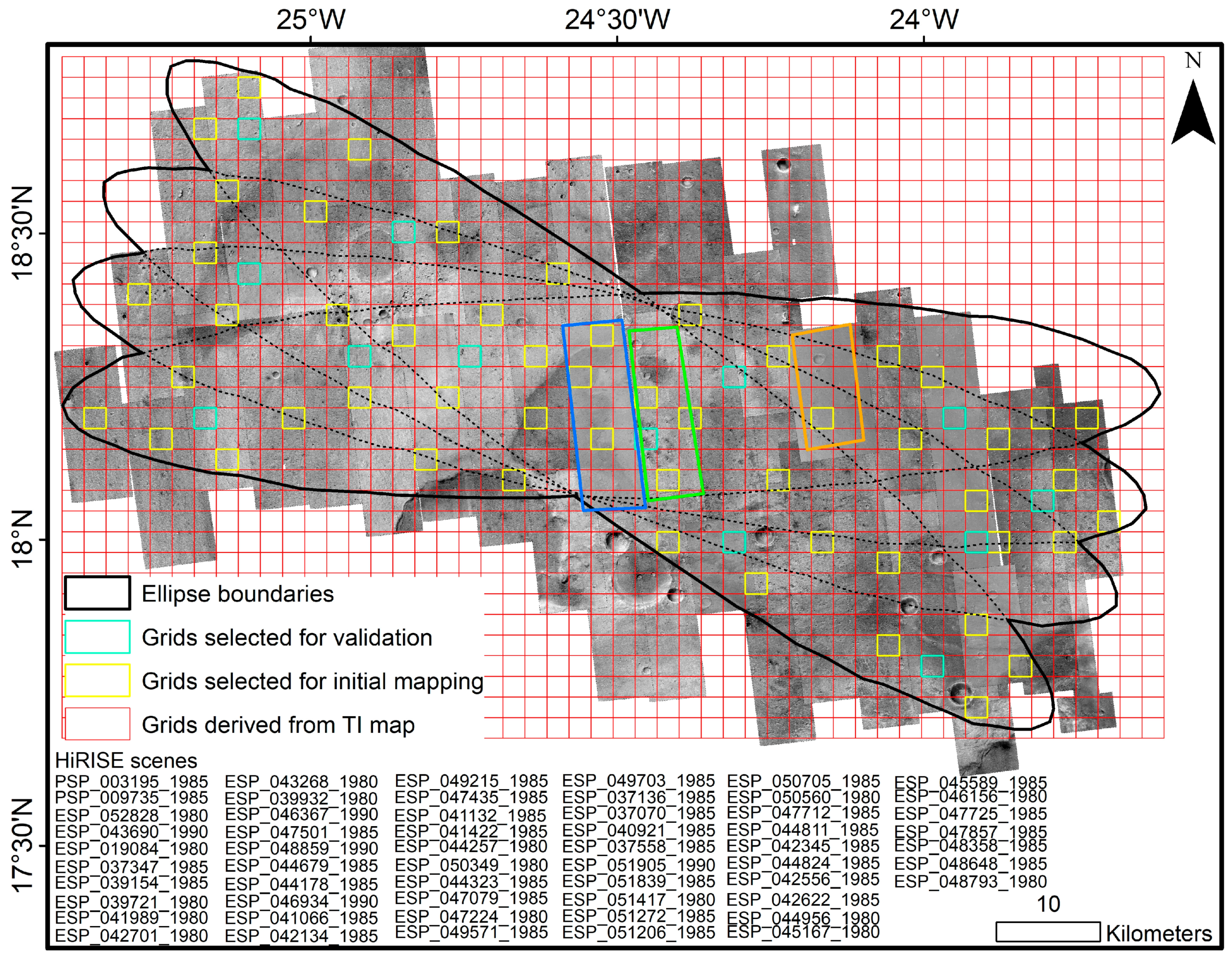
For the purpose of rover surface mobility, it is not the one-off TARs which are significantly dangerous as they can be avoided using even the rover mast cameras. The main problem arises when the rover encounters the contiguous stretches of TARs which can be actually hazardous for the rover mobility. Such closely located TARs are predominant in Oxia Planum. However, in our mapping, we identified and mapped both the singular TARs and the contiguous stretches of TARs in the selected grids. We used “Create Fishnet” tool of ArcGIS software and provided TES TI raster (Figure 1c) as the “template extent” dataset to derive corresponding grids of 2 × 2 km2 dimensions (Figure 2). As mentioned above, our study area is the region within the ellipse boundaries and therefore, to have a representative, balanced analysis of this wide region, we selected 66 grids uniformly distributed throughout the ellipses (Figure 2) and covering a total area of 264 km2 for HiRISE-based TAR mapping. In total, 57 sub-meter resolution HiRISE scenes (Figure 2) were selected to form the composite that covered nearly all of the study area and assisted in TAR mapping. We used the physical account well-described in the literature [5,10,38] to identify TARs in the images. TARs characteristically form in groups of tens to thousands of individual units and can easily be characterized by their small, narrow, and transverse dimensions, and elongated form [10]. Slip faces are typically resolvable only in high-resolution HiRISE images, and the opposite slopes appear to be nearly symmetric [5,10,38].
Although our mapping grids were well-distributed across the study area and since TARs are known to usually form in groups [10], the expected results were sufficient to provide an acceptable first-hand assessment and information about TAR distribution across the region. However, the facts that TARs typically form in contiguous stretches and that such spatially correlated TARs were abundant in the study area also suggested that we further perform spatial interpolation using the information from the mapped grids to derive a spatially continuous TAR distribution map. For this, we selected 53 of the mapped grids (yellow grids in Figure 2) and used “Kriging” interpolator [39] in ArcGIS. Kriging is one of the best geostatistical interpolation techniques in soil science and geology [40] and is well-explored to interpolate Martian regolith parameters [27] as it considers both the degree of variation between known data points and the distance between them while estimating values in unknown areas. Kriging is based on the assumption that the distance and direction between sample points reflect a spatial correlation that can be further exploited to predict the variation in the surface [40]. We subsequently used the remaining uniformly distributed 13 grids (cyan grids in Figure 2) to evaluate the performance of the interpolation process. Upon quantifying the spatial uncertainty in the interpolation, all 66 grids were employed for deriving the final TAR distribution map for the study area.
3.2. Morphology
The morphological interpretations for the TARs in the study area were based on visually identifying the first-order crest-ridge plan view morphological forms (simple, forked, wavy, barchan-like, and networked) described in the literature [10]. We characterized the most common morphologies of TARs in the region.
3.3. Morphometry
We used all the three available HiRISE digital terrain models (DTMs) for the study area: (1) DTEEC_003195_1985_002694_1985_L01, (2) DTEEC_009880_1985_009735_1985_L01, (3) DTEEC_036925_1985_037558_1985_L01 and the corresponding images to perform high-resolution (~1 m/pixel) morphometry of several TARs. The HiRISE DTMs produced by the HiRISE team are reliable with the reported vertical precision of a few tenths of a meter as a result of a stereo matching precision of about 0.2 of a pixel [41].
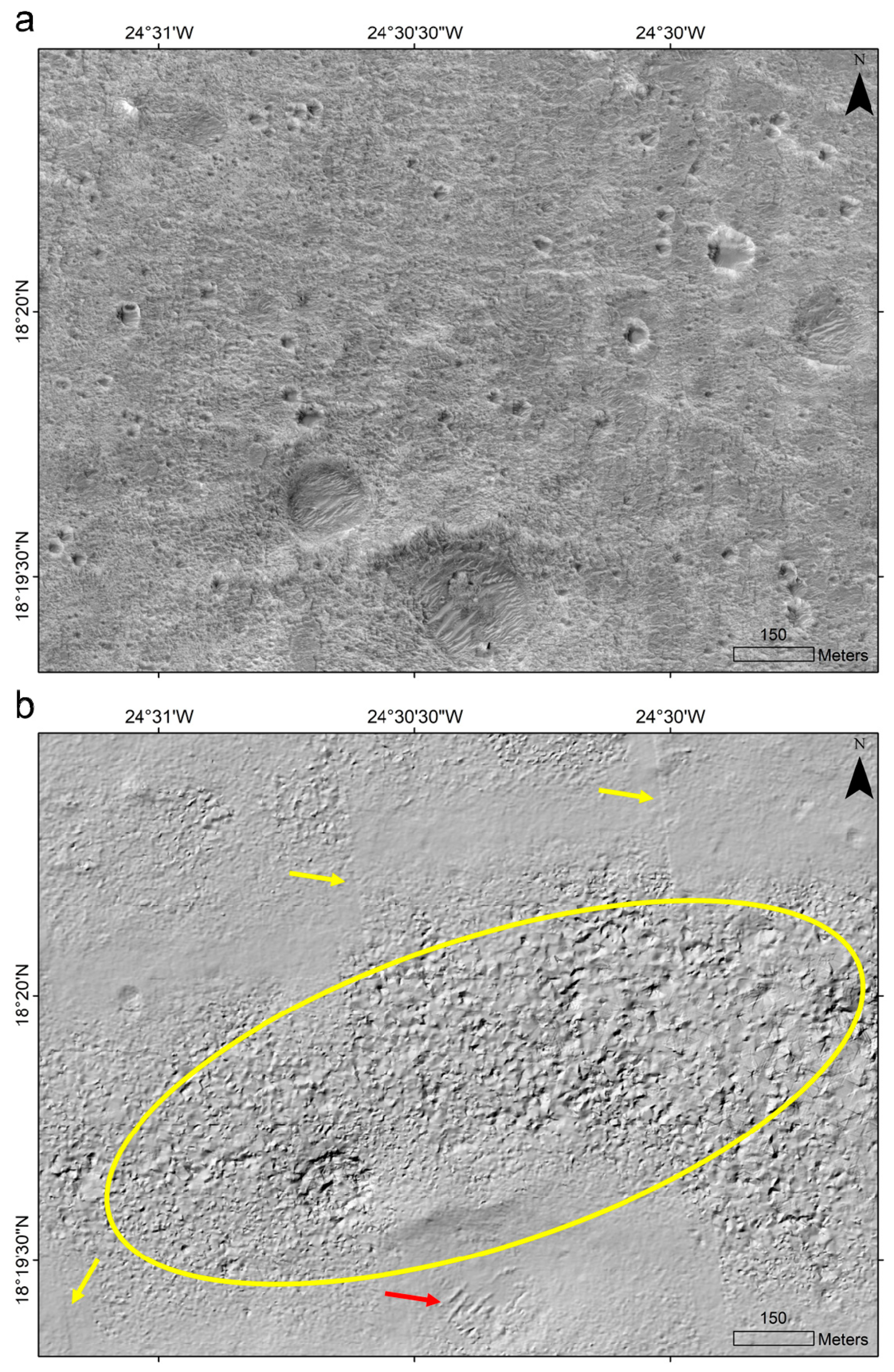
We further searched for the inherent noise within the used HiRISE DTMs [42]. There are mainly four such artifacts as reported by the HiRISE team [43] and one needs to look into the terrain shaded relief to detect these: (1) boxes, (2) faceted areas, (3) charged coupled device (CCD) seams, and (4) manually interpolated areas. We scrutinized the three DTMs for such artifacts using terrain shaded relief views and were able to identify mainly two types of artifacts; faceted areas and CCD seams (Figure 3). In fact, these artifacts cover large portions of the above-mentioned DEMs. We ensured that we sample and analyze only those TARs which are away from any of these artifacts. The “Hillshade” tool of ArcGIS was used to derive the shaded relief. Thus, we selected 150 TARs which were well-discernible in HiRISE DTMs, away from any artifacts, and displayed different sizes.
In the same way as Hugenholtz et al. [25], we also restricted our morphometric analysis to only ‘simple’ TARs as defined by Balme et al. [10]. These simple TARs have well-defined morphologies with symmetrical slopes, a single crestline, clearly marked edges, and low sinuosity [25], making the measurements easier and more accurate. We selected and digitized the crestlines of only those TARs which were clearly distinguishable in both the HiRISE image and its corresponding shaded relief (e.g., TARs indicated by the red arrow in Figure 3) to ensure that their topography was resolved in the DTM.
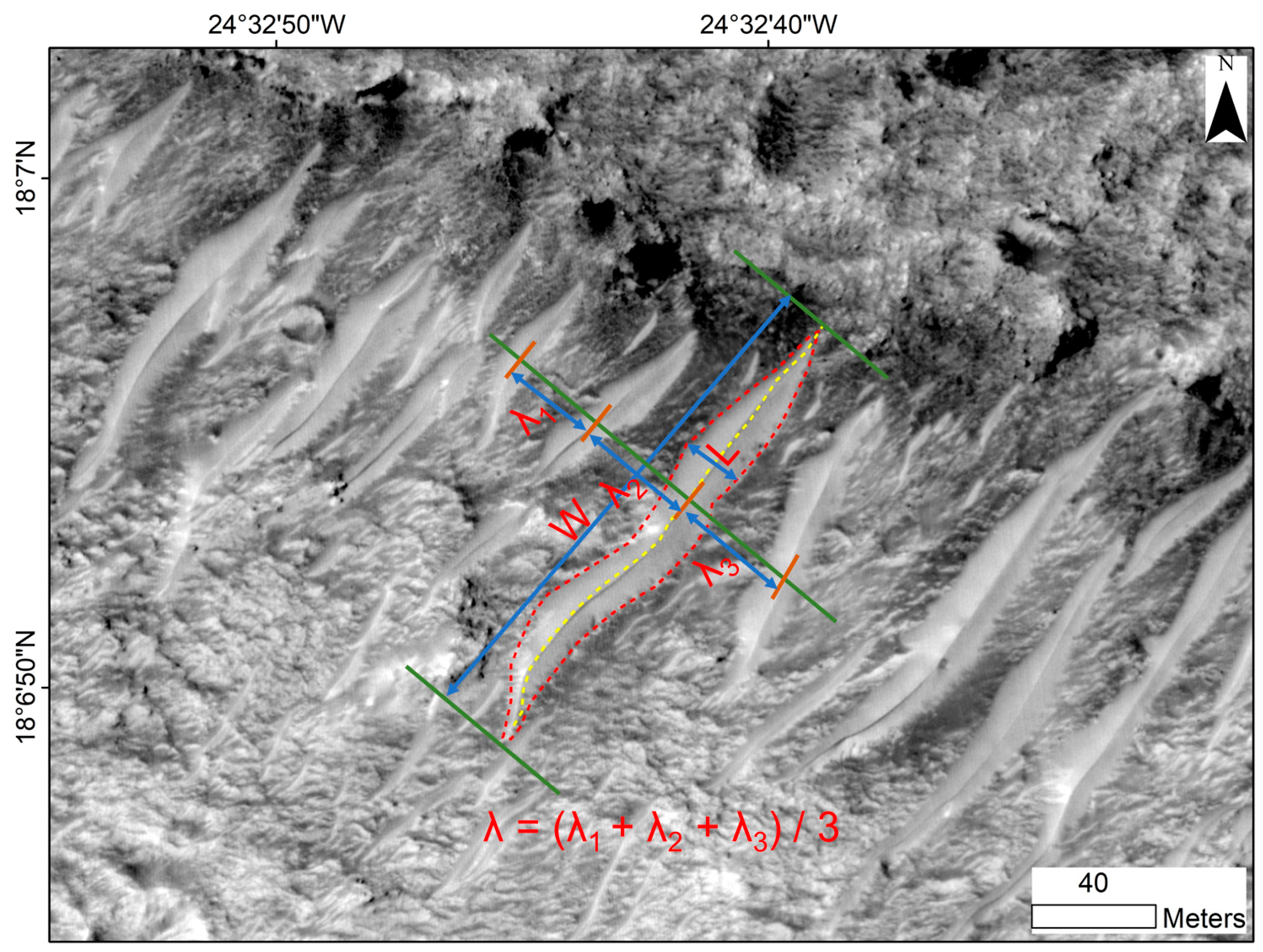
As defined by Balme et al. [10], TARs can be characterized by five morphometric parameters: (1) the crest-ridge width (W), (2) the down-wind TAR length (L), (3) the ridge-to-ridge mean spacing (λ), (4) plan view aspect ratio (a), where a = W/L, and (5) inter-bedform spacing (s), where s = λ/L (see Figure 4 for an illustration of these parameters in one specific example). L, as we take it, is the widest part of the TAR and should actually be recorded as the maximum “down-wind TAR length”. Similarly, λ, as we measure it, is the average of distances between the consecutive TAR crestlines at approximately the middle of the TARs. In addition to calculating these parameters for the selected TARs, we also derived along-crestline and across-crestline elevation profiles for several of them. However, we do not limit ourselves only to these morphometric parameters, but we also derive slope, orientation, and heights (h) for the selected TAR samples. The Pythagoras’ theorem was used for the h calculations and for the ease of understanding along with the transect analysis results, the description of height estimation is provided in Section 4.3. TAR orientations (N-S, NE-SW, NW-SE, or E-W) were analyzed based on the azimuthal position of TAR crest-ridge width.
4. Results and Discussion
The following sections summarize the key results of our study within the predefined objectives and we discuss the results in view of the previous studies.
4.1. TAR Distribution
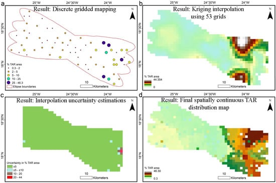
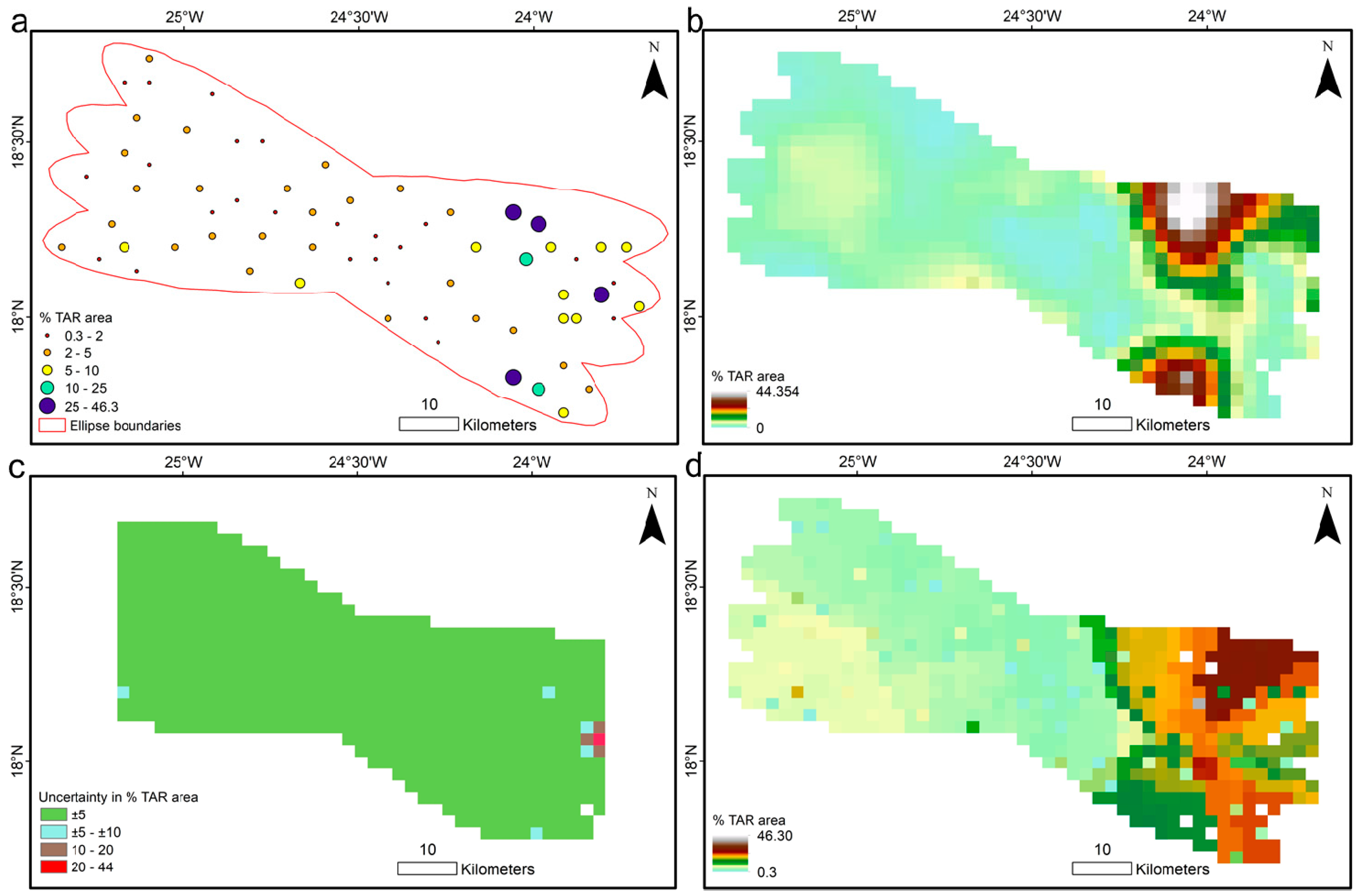
We present the gridded TAR mapping results in Figure 5. The % TAR area within each grid varies between 0.3% and 46.3% with a mean value of 5.78% and a standard deviation of 9.13% (Figure 5a). The result of Kriging interpolation using the first 53 mapped grids (Figure 2) is shown in Figure 5b. Two distinct nodes of high TAR density in the eastern margin of the study area are clearly observed (Figure 5b). The % TAR area varies between 0% and 44.354% with a mean value of 5.66% and a standard deviation of 6.97% (Figure 5b). The remaining 13 mapped grids (Figure 2) were selected as the validation dataset to evaluate the performance of the interpolator. Owing to the uniform distribution of the used grids for interpolation, the observed uncertainty (i.e., actual % area, interpolated % area) in interpolation was significantly less with a mean value of 3.27% and a standard deviation of 12.47% of the grid area. We further used these evaluation grids to interpolate the uncertainty across the study area and observed that for ~98.4% of the terrain the uncertainty was within ±5% of the grid area (Figure 5c). We observed the highest uncertainty of ~44% for one of the eastern-most grids and uncertainty values in the range of 5%–20% for the surrounding grids (Figure 5c). With such good interpolation results, we repeated the spatial interpolation using all the 66 mapped grids to derive the final TAR distribution map for the study area (Figure 5d). The % TAR area in the final TAR distribution map varied between 0.3% and 46.3% and the mean % TAR area for the region was 5.39% with a standard deviation of 4.87%.
As visible in Figure 5d, the TAR density and areal coverage is significantly higher towards the eastern margin of the study area as compared to the rest of the region. In fact, 63.5% of the region shows % TAR coverage of <5% and 80.32% of the study area displays <10% TAR coverage. There are very few conference abstracts [34,44] and one MPhil thesis [45], which have presented some results on partial gridded mapping of TARs in the region and our results are in good agreement with those studies. For example, Bridges et al. [44] presented TAR mapping results for 180 km2 (~5.6% of the study area) at 1:2000 scale (the same scale as selected by us) and reported an average TAR coverage of 4.1% with a very high (≤43%) TAR coverage towards the eastern margin. Our results for the entire study area (3211.07 km2) also show a mean TAR coverage of 5.39% with highest mean areal coverage of ~43% in the eastern margin. Bridges et al. [34] presented the updated results of TAR mapping for the study area and reported a mean TAR coverage of 4.4% for the sampled and mapped grids. Henson [45], for several more of the grids in the study area, reported an average TAR coverage of 4.9% ± 5.9%. Henson [45] also reported the highest TAR coverage of 42.7% (close to our estimate of 46.3%) in the east and the lowest overall coverage of 0.4% (close to 0.3% as we report). Our TAR estimates are in good agreement with the ones provided by other researchers which further suggest the effectiveness of our mapping and spatial interpolation and provide a holistic spatially continuous distribution of TAR across the region. In summary, Figure 5d is a reliable estimate of the distribution of TARs within the ExoMars landing ellipses in Oxia Planum, which can be used for surface operation planning and EDL assessment. It can also be used to compare with global and meso-scalar atmospheric circulation models to understand the role of present-day aeolian processes on the distribution and orientation of these landforms. We further tried to compare the TI values with TAR areal coverage for the respective grids, and as reported by previous studies for other regions on Mars [17,26], we too did not observe any direct correlation between the two. On an average, for <20% of the grid coverage by TARs, the observed TI was 393.94 Jm−2K−1s−1/2 while for >20% TAR coverage, the observed TI was 424.35 Jm−2K−1s−1/2. One interesting observation that we make is regarding the comparison between the TAR coverage (Figure 5d) and the rock abundance maps (Figure 1d). While, the eastern margin of the study area is abundant in TARs with lesser rock abundance, it is the middle-to-western part of the study area, which while having lesser TAR coverage, displays higher than average rock abundance with maximum values reaching up to 35.4% (Figure 1d). This means that the entire Oxia Planum region within the landing ellipses can pose serious challenges during the ExoMars 2020 landing and maneuvers as the presence of dense TARs and high rock abundance have nearly mutually exclusive spatial distribution and dangerous levels throughout the study area.
4.2. Morphology
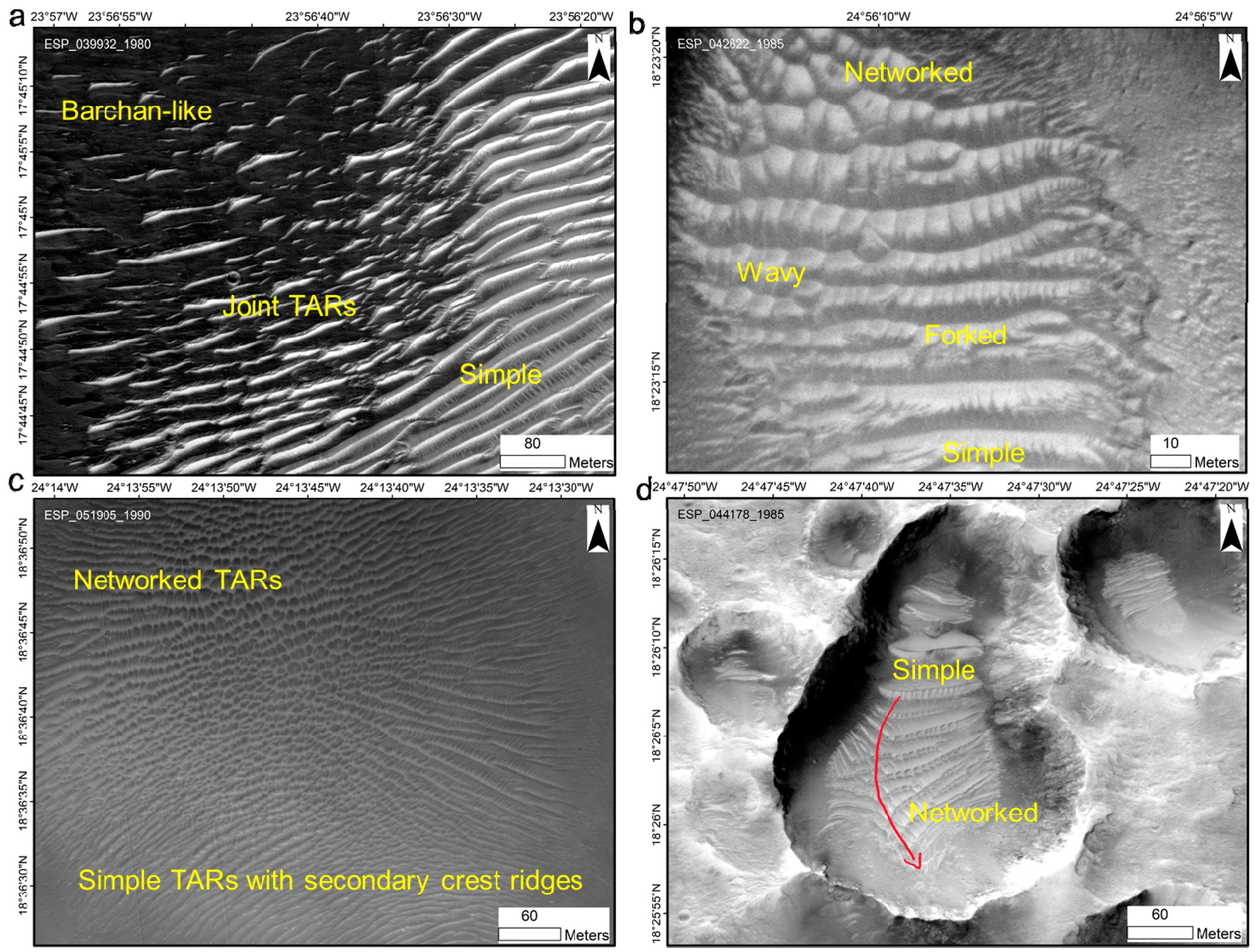
While performing the morphological observations, we were able to identify most of the first-order crest-ridge plan view morphologies of TARs as explained by Balme et al. [10], including the mini-TARs [31] in the study area (Figure 6). We have not focused on several other reported morphologies such as “raked pattern TARs” [46] and “dust drifts” [16]. The most prevalent morphology is simple TAR, abundantly present throughout the study area. This is followed by the forked TARs, which although significantly lesser in number than the simple TARs, are as abundant on the crater floors as outside the craters. The wavy, barchan-like, and networked morphologies are rare in the study area and are mainly present on the crater floors. Sometimes all or a combination of these five morphologies can co-exist within the same TAR deposit [10]. For example, in the study area, the forked and wavy morphologies with associated smaller secondary ripples are found to be co-existing mostly with simple morphologies. The barchan-like morphologies are found encompassing other morphologies within several of the crater floors. The mini-TARs are abundant in two regions, the eastern margin as well as the south-west region, with usually NE-SW orientations. Figure 6f can be used for comparison purposes between TARs and mini-TARs, which are about an order of magnitude smaller [31]. Balme et al. [31] have explained these mini-TARs to be potentially more hazardous for a rover as they are located in dense clusters.
We also observed several examples of TAR transitions as reported by Balme et al. [10] for the Meridiani region. Figure 7a highlights one case where barchan-like TARs coalesce to form joint and simple TARs through merging of their crest ridges. These barchan-like TARs usually display crest-ridge widths (W) of ~20–50 m and down-wind TAR lengths (L) of ~10–15 m. The simple TARs which they form can display average W of ~500 m. However, this transition is rare in the study area. Spatial transitions from simple, forked, and wavy TARs into networked TARs are relatively common in the study area (Figure 7b–d). In Figure 7b, we observe gradual transitions from simple to forked to wavy, and ultimately to networked morphologies. Figure 7c presents a case where secondary ridge crests forming approximately perpendicular to the largest simple TAR crest ridges display a transition to networked TARs. These TARs with secondary ridge crests are also called “feathered” TARs by Bourke et al. [18]. The W of these feathered TARs in the study area usually vary between 200–400 m. Figure 7d presents an interesting case of transition from simple to networked morphology as a possible combination of downslope winds and steep topography. Figure 7d also shows an elongated depression as a result of two merged craters. The shadows on the left suggest the topographic gradient with higher elevations in the smaller crater and gradual deepening towards the larger crater. Moving downslope from the border of the merged craters to the center of the larger crater, the simple TARs start showing transition and change in orientation along the marked red arrow (Figure 7d).
4.3. Morphometry
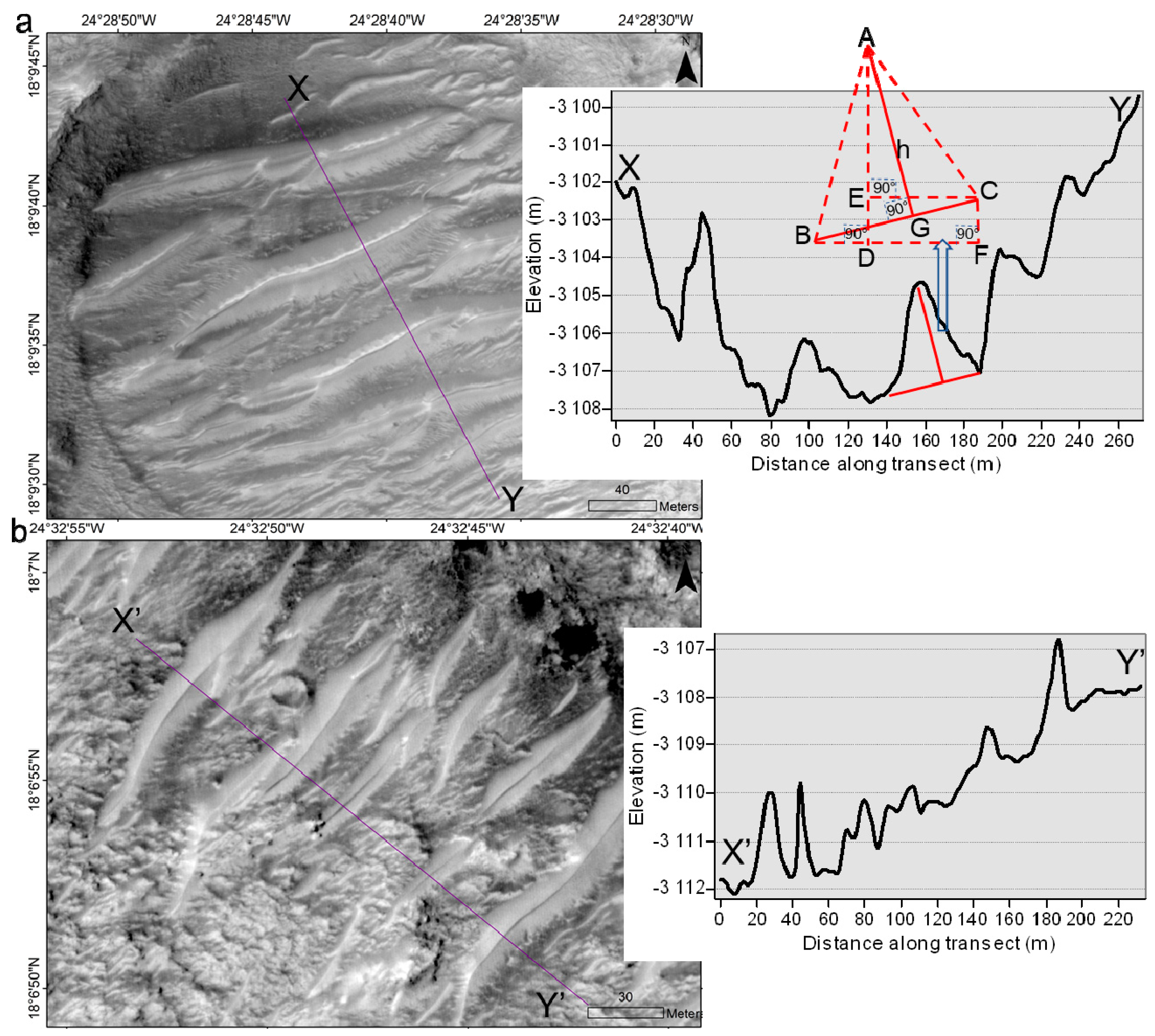
To our knowledge, we did not find any research paper which exclusively provides published accounts of TAR morphometrics in Oxia Planum. In addition to the conventional TAR morphometric parameters (W, L, λ, a, and s) as defined by Balme et al. [10], we also derived slope, orientation, and heights for the selected TAR samples. However, before we discuss the results, we would reiterate that the selected TAR samples for this analysis are representative of only simple TAR morphologies in the study area. Figure 8 presents two of the transects which were used to derive height (h) of 50 TARs with clearly distinct crests and troughs. The Pythagoras’ theorem was used for the h calculations (Figure 8a). BF (i.e., L), BD, and EC in Figure 8a can directly be derived using the planimetric measurements on the HiRISE images. Similarly, elevation differencing between the two points on the DTMs can directly provide AE, CF and AD. Afterwards, using the Equations (1) to (6), we can derive h. We have five right-angled triangles in Figure 8a to derive the required height (h); ∆CFB, ∆ADB, ∆AEC, ∆AGB, and ∆AGC. From these right-angled triangles, we can derive the following equations:
BC = (BF2 + CF2)1/2,
AB = (BD2 + AD2)1/2,
AC = (AE2 + EC2)1/2,
h = (AC2 − GC2)1/2 = (AC2 − (BC − BG)2)1/2,
h = (AB2 − BG2)1/2,
By equating Equations (4) and (5) we get;
(AB2 − BG2) = (AC2 − (BC − BG)2) => AB2 − AC2 + BC2 = 2BC.BG
=> BG = (AB2 − AC2 + BC2)/2BC,
=> BG = (AB2 − AC2 + BC2)/2BC,
Now, we can calculate the equivalent of BG from Equation (6) using values of AB, AC, and BC derived from Equations (1)–(3). When we put this value of BG in Equation (5), we can derive the value of h.
The study area is full of small TARs with λ = 2–3 m or L = 2–3 m [45]. Even in our samples which were chosen based on their clear visibility in HiRISE DTM shaded reliefs, we were able to characterize a TAR with L = 3.7 m (Table 1). Similarly, our other estimations regarding various TAR morphometrics are in good agreement with the ones reported for other regions by previous researchers. For example, Hugenholtz et al. [25], for 2295 TAR samples from across the mid and equatorial Martian latitudes, reported typical median morphometrics as W = 88.5 m, L = 17.3 m, h = 1.3 m, and λ = 25.8 m. Hugenholtz et al. [25] also stated the corresponding maximum (minimum) values for these parameters as W = 561.0 m (12.8 m), L = 77.5 m (1.5 m), h = 6.4 m (0. 2 m), and λ= 140.5 m (5.9 m), respectively. Bourke et al. [38] reported TAR heights (h) in the range of 1–7.8 m. Wilson and Zimbelman [2] analyzed 340 TAR samples in 172 MOC images and reported mean λ = ∼40 m, L = 10–60 m, mean W = 215 m (with a standard deviation of 155 m). For the morphometric analysis of ~500 TARs, Berman et al. [11] stated average median values for h (1.3 m), L (22.8 m), and λ (35.6 m). Geissler and Wilgus [17] for an analysis made on 154 DTMs reported maximum h = 14 m (mean h = 2.6 m with a standard deviation of 1.4 m) and maximum λ = 120 m (mean λ = 47.1 m with a standard deviation of 25.9 m). Shockey and Zimbelman [47] for 60 transect profiles reported average L = 22.6 m (maximum L = 107 m and minimum L = 4.5 m) with majority of L in the range of 15 to 30 m. They also reported average h = 2.3 m (maximum h = 9.7 m and minimum h = 0.3 m) majority of h in the range 0.5 to 5 m. Regarding the average slopes of TAR flanks, Berman et al. [11] reported a range of ~3–10°, while Shockey and Zimbelman [47] and Zimbelman [20] reported the average slopes to be 14.5° and ~15°, respectively. All these dimensions and morphometrics are of a similar order of magnitude and nature as observed by us in Oxia Planum (Table 1) for a localized and smaller TAR population. We found a wide variability of TAR dimensions across the three DTMs within the study area with up to a factor of ~7–10 difference in TAR morphometrics as also reported by Geissler and Wilgus [17]. Overall, we report the average TAR morphometrics (±standard deviation) of W = 131.1 m (±106.2 m), L = 17.6 m (±10.1 m), λ = 37.3 m (±11.6 m), a = 7.1 (±2.3), s = 2.1 (±1.1), slope = 10.6° (±6.1°), predominant orientations of NE-SW and E-W, and h = 1.2 m (±0.8 m) (Table 1). Usually the longer TARs are wider too in most of the instances, but we did not observe any prevalent or statistically significant relationships of the W and L with the h dimensions of TARs in the study area as also evident from the transect profiles in Figure 8.
5. Conclusions
The present research provides first-hand detailed information about the distribution, morphologies, and morphometrics of TARs in the ExoMars 2020 landing site within Oxia Planum. TARs are widespread aeolian landforms on contemporary Mars, but we are yet to be certain of their formation mechanism, age and temporal evolution, composition and geophysics, and their relationship with global sedimentation and climatic evolution. Thus, although the presence of TARs in the study area with a particularly high density in the entire eastern margin of the landing ellipses poses a significant potential threat to the ExoMars 2020 mission, it also equips us with a unique opportunity to investigate these enigmatic landforms at unprecedented spectral resolutions and corroborate the results with precise meteorological parameters. The rover platform is equipped with infrared spectrometers and multispectral imagers, and the provision of a drill with an embedded multispectral camera provides us the opportunity to perform profiling starting from the tougher top layer of TARs and reaching to the supposedly loosely-packed subsurface. Considering that the drill can reach up to a maximum depth of 2 m and the average TAR height reported by us is 1.25 m, we can actually aim towards the complete profiling of a given TAR in terms of its composition and sedimentation. Although the TARs in Oxia Planum are similar in their dimensions to the TARs reported from other regions, we identify a strong NE-SW and E-W orientation for a majority of them. The presence of dense populations of mini-TARs in the region will be an additional challenge for the rover maneuvers as the maximum height of these mini-TARs can reach up to 25 cm [31] and they cannot be characterized using HiRISE DTMs. One of the most useful products of future studies could be a map of all TAR crestlines in the study area with their orientation represented as a rose plot. In the present work, the crestline analysis was part of our morphometric analyses which we performed only for selected 150 TARs, which were clearly represented in the DTMs. Performing such a directional analysis for all the TAR crestlines in the study area will take a considerable effort. Additionally, given the highly variable morphologies in this vast area, we will have to first fix some set of rules to perform such a directional analysis and it can be considered as one of the future scopes of the present work. In summary, our results can prove to be useful for ExoMars surface operation planning and EDL assessment. Furthermore, such studies are of interest to compare with global and meso-scalar atmospheric circulation models to understand the role of present-day aeolian processes on the distribution and orientation of TARs. Future observations from the ExoMars Rover and surface platform will provide ground truth to these remote sensing and wind modeling analyses.
Author Contributions
Conceptualization, A.B.; formal analysis, A.B., L.S., F.J.M.-T. and M.-P.Z.; funding acquisition, F.J.M.-T. and M.-P.Z.; investigation, A.B., L.S., F.J.M.-T. and M.-P.Z.; methodology, A.B. and L.S.; software, A.B. and L.S.; writing—original draft, A.B.; writing—review and editing, L.S., F.J.M.-T. and M.-P.Z.
Funding
This research received no external funding.
Acknowledgments
We thank the efforts of the guest editor and the reviewers for their suggestions in improving the paper. We acknowledge the Wallenberg Foundation and the Kempe Foundation for supporting our Mars research activities in general. We thank Scott Nowicki for providing us the TES-derived rock abundance global dataset for Mars. We thank NASA, JPL, and University of Arizona for providing HiRISE images and DTMs free of charge. The maps in various figures have been created using ArcGIS version 10.6.1 (http://desktop.arcgis.com/en/arcmap/latest/get-started/setup/arcgis-desktop-quick-start-guide.htm).
Conflicts of Interest
The authors declare no conflicts of interest. The funders had no role in the design of the study; in the collection, analyses, or interpretation of data; in the writing of the manuscript, or in the decision to publish the results.
References
- Craddock, R.A. Aeolian processes on the terrestrial planets: Recent observations and future focus. Progress Phys. Geogr. 2012, 36, 110–124. [Google Scholar] [CrossRef]
- Wilson, S.A.; Zimbelman, J.R. Latitude-dependent nature and physical characteristics of transverse aeolian ridges on Mars. J. Geophys. Res. Planets 2004, 109, E10003. [Google Scholar] [CrossRef]
- McCauley, J.F.; Carr, M.H.; Cutts, J.A.; Hartmann, W.K.; Masursky, H.; Milton, D.J.; Sharp, R.P.; Wilhelms, D.E. Preliminary Mariner 9 report on the geology of Mars. Icarus 1972, 17, 289–327. [Google Scholar] [CrossRef]
- Cutts, J.A.; Blasius, K.R.; Briggs, G.A.; Carr, M.H.; Greeley, R.; Masursky, H. North polar region of Mars: Imaging results from Viking 2. Science 1976, 194, 1329–1337. [Google Scholar] [CrossRef] [PubMed]
- Malin, M.C.; Edgett, K.S. Mars Global Surveyor Mars Orbiter Camera: Interplanetary cruise through primary mission. J. Geophys. Res. 2001, 106, 23429–23570. [Google Scholar] [CrossRef] [Green Version]
- Neukum, G.; Jaumann, R. HRSC: The High Resolution Stereo Camera of Mars Express, Mars Express: The Scientific Payload; Wilson, A., Chicarro, A., Eds.; ESA Publications Division: Noordwijk, The Netherlands, 2004; pp. 17–35. ISBN 92-9092-556-6. [Google Scholar]
- Malin, M.C.; Bell, J.F.; Cantor, B.A.; Caplinger, M.A.; Calvin, W.M.; Clancy, R.T.; Edgett, K.S.; Edwards, L.; Haberle, R.M.; James, P.B.; et al. Context Camera Investigation on board the Mars Reconnaissance Orbiter. J. Geophys. Res. Planets 2007, 112. [Google Scholar] [CrossRef] [Green Version]
- McEwen, A.S.; Eliason, E.M.; Bergstrom, J.W.; Bridges, N.T.; Hansen, C.J.; Delamere, W.A.; Grant, J.A.; Gulick, V.C.; Herkenhoff, K.E.; Keszthelyi, L.; et al. Mars reconnaissance orbiter’s high resolution imaging science experiment (HiRISE). J. Geophys. Res. Planets 2007, 112. [Google Scholar] [CrossRef]
- Bhardwaj, A.; Sam, L.; Martín-Torres, F.J.; Zorzano, M.P. Are Slope Streaks Indicative of Global-Scale Aqueous Processes on Contemporary Mars? Rev. Geophys. 2019, 57, 48–77. [Google Scholar] [CrossRef]
- Balme, M.; Berman, D.C.; Bourke, M.C.; Zimbelman, J.R. Transverse aeolian ridges (TARs) on Mars. Geomorphology 2008, 101, 703–720. [Google Scholar] [CrossRef]
- Berman, D.C.; Balme, M.R.; Michalski, J.R.; Clark, S.C.; Joseph, E.C. High-resolution investigations of Transverse Aeolian Ridges on Mars. Icarus 2018, 312, 247–266. [Google Scholar] [CrossRef]
- Hayward, R.K.; Mullins, K.F.; Fenton, L.K.; Hare, T.M.; Titus, T.N.; Bourke, M.C.; Colaprete, A.; Christensen, P.R. Mars global digital dune database and initial science results. J. Geophys. Res. Planets 2007, 112. [Google Scholar] [CrossRef]
- Silvestro, S.; Vaz, D.A.; Fenton, L.K.; Geissler, P.E. Active aeolian processes on Mars: A regional study in Arabia and Meridiani Terrae. Geophys. Res. Lett. 2011, 38. [Google Scholar] [CrossRef] [Green Version]
- Vaz, D.A.; Silvestro, S. Mapping and characterization of small-scale aeolian structures on Mars: An example from the MSL landing site in Gale Crater. Icarus 2014, 230, 151–161. [Google Scholar] [CrossRef] [Green Version]
- Ward, A.W.; Doyle, K.B.; Helm, P.J.; Weisman, M.K.; Witbeck, N.E. Global map of eolian features on Mars. J. Geophys. Res. Solid Earth 1985, 90, 2038–2056. [Google Scholar] [CrossRef]
- Geissler, P.E. The birth and death of transverse aeolian ridges on Mars. J. Geophys. Res. Planets 2014, 119, 2583–2599. [Google Scholar] [CrossRef] [Green Version]
- Geissler, P.E.; Wilgus, J.T. The morphology of transverse aeolian ridges on Mars. Aeolian Res. 2017, 26, 63–71. [Google Scholar] [CrossRef]
- Bourke, M.C.; Wilson, S.A.; Zimbelman, J.R. The variability of TARs in troughs on Mars. In Proceedings of the 34th Lunar and Planetary Science Conference, Clear Lake City, Houston, TX, USA, 17–21 March 2003. Abstract number 2090. [Google Scholar]
- Foroutan, M.; Zimbelman, J.R. Mega-ripples in Iran: A new analog for transverse aeolian ridges on Mars. Icarus 2016, 274, 99–105. [Google Scholar] [CrossRef]
- Zimbelman, J.R. Transverse Aeolian ridges on Mars: First results from HiRISE images. Geomorphology 2010, 121, 22–29. [Google Scholar] [CrossRef]
- De Silva, S.L.; Spagnuolo, M.G.; Bridges, N.T.; Zimbelman, J.R. Gravel-mantled megaripples of the Argentinean Puna: A model for their origin and growth with implications for Mars. Geol. Soc. Am. Bull. 2013, 125, 1912–1929. [Google Scholar] [CrossRef]
- Hugenholtz, C.H.; Barchyn, T.E. A terrestrial analog for transverse aeolian ridges (TARs): Environment, morphometry, and recent dynamics. Icarus 2017, 289, 239–253. [Google Scholar] [CrossRef]
- Foroutan, M.; Steinmetz, G.; Zimbelman, J.R.; Duguay, C.R. Megaripples at Wau-an-Namus, Libya: A new analog for similar features on Mars. Icarus 2019, 319, 840–851. [Google Scholar] [CrossRef]
- Zimbelman, J.R.; Scheidt, S.P. Precision topography of a reversing sand dune at Bruneau Dunes, Idaho, as an analog for transverse aeolian ridges on Mars. Icarus 2014, 230, 29–37. [Google Scholar] [CrossRef]
- Hugenholtz, C.H.; Barchyn, T.E.; Boulding, A. Morphology of transverse aeolian ridges (TARs) on Mars from a large sample: Further evidence of a megaripple origin? Icarus 2017, 286, 193–201. [Google Scholar] [CrossRef]
- Berman, D.C.; Balme, M.R.; Rafkin, S.C.; Zimbelman, J.R. Transverse aeolian ridges (TARs) on Mars II: distributions, orientations, and ages. Icarus 2011, 213, 116–130. [Google Scholar] [CrossRef]
- Bhardwaj, A.; Sam, L.; Martín-Torres, F.J.; Zorzano, M.P. Discovery of recurring slope lineae candidates in Mawrth Vallis, Mars. Sci. Rep. 2019, 9. [Google Scholar] [CrossRef]
- Sullivan, R.; Arvidson, R.; Bell, J.F., III; Gellert, R.; Golombek, M.; Greeley, R.; Herken-hoff, K.; Johnson, J.; Thompson, S.; Whelley, P.; et al. Wind-driven particle mobility on Mars: Insights from Mars exploration observations at ‘‘El Dorado’’ and surroundings at Gusev Crater. J. Geophys. Res. 2008, 113, E06S07. [Google Scholar] [CrossRef]
- Sullivan, R.; Bridges, N.; Herkenhoff, K.; Hamilton, V.; Rubin, D. Transverse Aeolian ridges (TARs) as megaripples: Rover encounters at Meridiani Planum, Gusev, and gale. In Proceedings of the Eighth International Conference on Mars, Pasadena, CA, USA, 14–18 July 2014; LPI Contribution No. 1791. p. 1424. Available online: https://www.hou.usra.edu/meetings/8thmars2014/pdf/1424.pdf (accessed on 10 February 2019).
- Arvidson, R.E.; Iagnemma, K.D.; Maimone, M.; Fraeman, A.A.; Zhou, F.; Heverly, M.C.; Bellutta, P.; Rubin, D.; Stein, N.T.; Grotzinger, J.P.; et al. Mars science laboratory curiosity rover megaripple crossings up to sol 710 in Gale Crater: curiosity rover megaripple crossings. J. Field Robot. 2017, 34, 495–518. [Google Scholar] [CrossRef]
- Balme, M.; Robson, E.; Barnes, R.; Butcher, F.; Fawdon, P.; Huber, B.; Ortner, T.; Paar, G.; Traxler, C.; Bridges, J.; et al. Surface-based 3D measurements of small aeolian bedforms on Mars and implications for estimating ExoMars rover traversability hazards. Planet. Space Sci. 2018, 153, 39–53. [Google Scholar] [CrossRef] [Green Version]
- Arvidson, R.E.; Ashley, J.W.; Bell, J.F.; Chojnacki, M.; Cohen, J.; Economou, T.E.; Farrand, W.H.; Fergason, R.; Fleischer, I.; Geissler, P.; et al. Opportunity Mars Rover mission: overview and selected results from Purgatory ripple to traverses to Endeavour crater. J. Geophys. Res. Planets 2011, 116. [Google Scholar] [CrossRef]
- Arvidson, R.E.; Bell, J.F.; Bellutta, P.; Cabrol, N.A.; Catalano, J.G.; Cohen, J.; Crumpler, L.S.; Des Marais, D.J.; Estlin, T.A.; Farrand, W.H.; et al. Spirit Mars rover mission: overview and selected results from the northern home plate Winter haven to the side of Scamander crater. J. Geophys. Res. Planets 2010, 115. [Google Scholar] [CrossRef]
- Bridges, J.C.; Bowen, A.P.; Fawdon, P.; Balme, M.; Vago, J.; Hauber, E.; Loizeau, D.; Williams, R.M.E.; Sefton-Nash, E.; Turner, S.M.R.; et al. ExoMars 2020 landing site selection and characterization. In Proceedings of the 49th Lunar and Planetary Science Conference 2018 (LPI Contrib. No. 2083), The Woodlands, TX, USA, 19–23 March 2018; Available online: https://www.hou.usra.edu/meetings/lpsc2018/pdf/2177.pdf (accessed on 10 February 2019).
- Quantin, C.; Carter, J.; Thollot, P.; Broyer, J.; Lozach, L.; Davis, J.; Grindrod, P.; Pajola, M.; Baratti, E.; Rossato, S.; et al. Oxia Planum, the landing site for ExoMars 2018. In Proceedings of the 47th Lunar and Planetary Science Conference, The Woodlands, TX, USA, 21–25 March 2016; Abstract number 2863. Available online: https://www.hou.usra.edu/meetings/lpsc2016/pdf/2863.pdf (accessed on 10 February 2019).
- Putzig, N.E.; Mellon, M.T. Apparent thermal inertia and the surface heterogeneity of Mars. Icarus 2007, 191, 68–94. [Google Scholar] [CrossRef]
- Nowicki, S.A.; Christensen, P.R. Rock abundance on Mars from the Thermal Emission Spectrometer. J. Geophys. Res. Planets 2007, 112. [Google Scholar] [CrossRef] [Green Version]
- Bourke, M.C.; Balme, M.R.; Beyer, R.A.; Williams, K.K.; Zimbelman, J. A comparison of methods used to estimate the height of sand dunes on Mars. Geomorphology 2006, 81, 440–452. [Google Scholar] [CrossRef] [Green Version]
- Burrough, P.A.; McDonell, R.A. Principles of Geographical Information Systems; Oxford University Press: New York, NY, USA, 1998; p. 190. [Google Scholar]
- Types of Interpolation Methods. Available online: http://www.gisresources.com/types-interpolation-methods_3/ (accessed on 20 November 2018).
- Kirk, R.L.; Howington-Kraus, E.; Rosiek, M.R.; Anderson, J.A.; Archinal, B.A.; Becker, K.J.; Cook, D.A.; Galuszka, D.M.; Geissler, P.E.; Hare, T.M.; et al. Ultrahigh resolution topographic mapping of Mars with MRO HiRISE stereo images: Meter-scale slopes of candidate Phoenix landing sites. J. Geophys. Res. Planet 2008, 113. [Google Scholar] [CrossRef] [Green Version]
- Bhardwaj, A.; Sam, L.; Martín-Torres, F.J.; Zorzano, M.P. Martian slope streaks as plausible indicators of transient water activity. Sci. Rep. 2017, 7. [Google Scholar] [CrossRef] [PubMed]
- Overview of Digital Terrain Models (DTM). Available online: https://www.uahirise.org/dtm/about.php (accessed on 20 November 2018).
- Bridges, D.; Loizeau, D.; Sefton-Nash, E.; Vago, J.; Williams, R.M.E.; Balme, M.; Turner, S.M.R.; Fawdon, P.; Davis, J.M.; The ExoMars Landing Site Selection Working Group. Selection and characterisation of the ExoMars 2020 rover landing sites. In Proceedings of the 48th Lunar and Planetary Science Conference 2017 (LPI Contrib. No. 2378), The Woodlands, TX, USA, 20–24 March 2017; Available online: https://www.hou.usra.edu/meetings/lpsc2017/pdf/2378.pdf (accessed on 10 February 2019).
- Henson, R.A. Remote Characterisation of Mars: Preparation for ExoMars. Master’s Thesis, University of Leicester, Leicester, UK, 2017. Available online: https://lra.le.ac.uk/bitstream/2381/39576/1/2017HENSONRAMPhil.pdf (accessed on 10 February 2019).
- Foroutan, M.; Zimbelman, J.R. Raked Pattern TARs: Evolution and Formation of a Unique Pattern in an Active Sediment Transport Environment. In Proceedings of the 2016 AGU Fall Meeting, San Francisco, CA, USA, December 2016; Available online: http://adsabs.harvard.edu/abs/2016AGUFMEP41B0906F (accessed on 9 April 2019).
- Shockey, K.M.; Zimbelman, J.R. Analysis of transverse aeolian ridge profiles derived from HiRISE images of Mars. Earth Surf. Process. Landf. 2013, 38, 179–182. [Google Scholar] [CrossRef]
Figure 1.
Oxia Planum as the study site for ExoMars 2020 landing. (a) Mars Orbiter Laser Altimeter (MOLA)-derived topography map of Mars showing location of Oxia Planum as the red dot (MOLA data courtesy: NASA/JPL/Goddard). (b) MOLA topography of Oxia Planum within expected landing ellipses (3-σ) [34]. (c) Mars Global Surveyor (MGS) Thermal Emission Spectrometer (TES)-derived thermal inertia [36] for Oxia Planum landing ellipses. (d) TES-derived % rock abundance [37] map for Oxia Planum landing ellipses.

Figure 2.
Oxia Planum in high-resolutions. A total of 57 high resolution imaging science experiment (HiRISE) scenes have been used to make the composite and perform the mapping. The orange, green, and blue rectangles highlight the regions with available HiRISE digital terrain models (DTMs) DTEEC_003195_1985_002694_1985_L01, DTEEC_036925_1985_037558_1985_L01, and DTEEC_009880_1985_009735_1985_L01.IMG, respectively. HiRISE image and DTM credit: NASA/JPL/University of Arizona.

Figure 3.
Common DTM artifacts. A region in Oxia Planum as seen in (a) HiRISE image PSP_009735_1985_RED and its corresponding (b) shaded relief derived from the DTM (DTEEC_009880_1985_009735_1985_L01; blue rectangle in Figure 2). The yellow ellipse highlights faceted areas and the yellow arrows highlight charged coupled device (CCD) seams. The red arrow shows clearly visible simple TARs. HiRISE image and DTM credit: NASA/JPL/University of Arizona.

Figure 4.
Elements of morphometry for transverse aeolian ridges (TARs) as seen in HiRISE image PSP_009735_1985. The red dashed curves represent the TAR boundary and the yellow curve represents the crestline. W = crest-ridge width, L = down-wind TAR length, λ = ridge-to-ridge mean spacing (wavelength). HiRISE image credit: NASA/JPL/University of Arizona.

Figure 5.
TAR distribution across the study area. (a) % TAR area within the mapped grids. (b) TAR distribution as areal % per grid spatially interpolated using 53 mapped grids. (c) % uncertainty in interpolated % TAR area estimated using 13 mapped grids. (d) Areal distribution of TARs based on spatial interpolation using all the 66 mapped grids.

Figure 6.
TAR morphologies in the study area: (a) simple TAR, (b) forked TAR, (c) wavy TAR with associated smaller secondary ripples, (d) barchan-like TAR, (e) networked TAR, and (f) mini-TARs. HiRISE image credit: NASA/JPL/University of Arizona.
Figure 6.
TAR morphologies in the study area: (a) simple TAR, (b) forked TAR, (c) wavy TAR with associated smaller secondary ripples, (d) barchan-like TAR, (e) networked TAR, and (f) mini-TARs. HiRISE image credit: NASA/JPL/University of Arizona.

Figure 7.
Examples of TAR transitions: (a) barchan-like TARs coalescing and forming simple TARs, (b) transition from simple to forked to wavy with associated smaller secondary ripples, and finally to networked TARs, (c) simple TARs with secondary crest ridges transitioning to networked TARs, and (d) downslope transitions from simple to networked along the red arrow possibly due to the combination of downslope winds and steep topography. HiRISE image credit: NASA/JPL/University of Arizona.

Figure 8.
Examples of transect (violet lines overlaid on HiRISE image) analysis and TAR height (h) estimations: (a) a transect for TARs with W >150 m and within a confined space (i.e., crater), (b) a transect for TARs in a relatively open space. The elevation profile is derived from the HiRISE DTM DTEEC_009880_1985_009735_1985_L01 and HiRISE image PSP_009735_1985 is in the background. HiRISE image and DTM credit: NASA/JPL/University of Arizona.


Table 1.
Morphometric parameters for the selected 150 TAR samples.
| Parameter (Unit) | Maximum | Minimum | Mean | Standard Deviation |
|---|---|---|---|---|
| 1. W (m) | 411 | 32.9 | 131.1 | 106.2 |
| 2. L (m) | 33.2 | 3.7 | 17.6 | 10.1 |
| 3. a | 13.2 | 4.5 | 7.1 | 2.3 |
| 4. λ (m) | 61.2 | 10.6 | 37.3 | 11.6 |
| 5. s | 1.8 | 2.9 | 2.1 | 1.1 |
| 6. Slope (degree) | - | - | 9.7 (W = >400 m) 11.2 (W = 200–400 m) 10.9 (W = <200 m) | 5.9 (W = >400 m) 6.8 (W = 200–400 m) 5.5 (W = <200 m) |
| 7. Predominant Orientations | - | - | NE-SW 1, E-W 2 | - |
| 8. Height (m) | 4.6 | 0.4 | 1.2 | 0.8 |
1 Northeast-southwest; 2 east-west.
© 2019 by the authors. Licensee MDPI, Basel, Switzerland. This article is an open access article distributed under the terms and conditions of the Creative Commons Attribution (CC BY) license (http://creativecommons.org/licenses/by/4.0/).
Share and Cite
MDPI and ACS Style
Bhardwaj, A.; Sam, L.; Martin-Torres, F.J.; Zorzano, M.-P. Distribution and Morphologies of Transverse Aeolian Ridges in ExoMars 2020 Rover Landing Site. Remote Sens. 2019, 11, 912. https://doi.org/10.3390/rs11080912
AMA Style
Bhardwaj A, Sam L, Martin-Torres FJ, Zorzano M-P. Distribution and Morphologies of Transverse Aeolian Ridges in ExoMars 2020 Rover Landing Site. Remote Sensing. 2019; 11(8):912. https://doi.org/10.3390/rs11080912
Chicago/Turabian StyleBhardwaj, Anshuman, Lydia Sam, F. Javier Martin-Torres, and Maria-Paz Zorzano. 2019. "Distribution and Morphologies of Transverse Aeolian Ridges in ExoMars 2020 Rover Landing Site" Remote Sensing 11, no. 8: 912. https://doi.org/10.3390/rs11080912
Note that from the first issue of 2016, this journal uses article numbers instead of page numbers. See further details here.