Evaluation of SMAP, SMOS-IC, FY3B, JAXA, and LPRM Soil Moisture Products over the Qinghai-Tibet Plateau and Its Surrounding Areas

Abstract

High-quality and long time-series soil moisture (SM) data are increasingly required for the Qinghai-Tibet Plateau (QTP) to more accurately and effectively assess climate change. In this study, to evaluate the accuracy and effectiveness of SM data, five passive microwave remotely sensed SM products are collected over the QTP, including those from the soil moisture active passive (SMAP), soil moisture and ocean salinity INRA-CESBIO (SMOS-IC), Fengyun-3B microwave radiation image (FY3B), and two SM products derived from the advanced microwave scanning radiometer 2 (AMSR2). The two AMSR2 products are generated by the land parameter retrieval model (LPRM) and the Japan Aerospace Exploration Agency (JAXA) algorithm, respectively. The SM products are evaluated through a two-stage data comparison method. The first stage is direct validation at the grid scale. Five SM products are compared with corresponding in situ measurements at five in situ networks, including Heihe, Naqu, Pali, Maqu, and Ngari. Another stage is indirect validation at the regional scale, where the uncertainties of the data are quantified by using a three-cornered hat (TCH) method. The results at the regional scale indicate that soil moisture is underestimated by JAXA and overestimated by LPRM, some noise is contained in temporal variations in SMOS-IC, and FY3B has relatively low absolute accuracy. The uncertainty of SMAP is the lowest among the five products over the entire QTP. In the SM map composed by five SM products with the lowest pixel-level uncertainty, 66.64% of the area is covered by SMAP (JAXA: 19.39%, FY3B: 10.83%, LPRM: 2.11%, and SMOS-IC: 1.03%). This study reveals some of the reasons for the different performances of these five SM products, mainly from the perspective of the parameterization schemes of their corresponding retrieval algorithms. Specifically, the parameterization configurations and corresponding input datasets, including the land-surface temperature, the vegetation optical depth, and the soil dielectric mixing model are analyzed and discussed. This study provides quantitative evidence to better understand the uncertainties of SM products and explain errors that originate from the retrieval algorithms.

1. Introduction

Soil moisture (SM) is a critical indicator of the water and energy budgets at the land surface, and a key variable that links the land surface and atmosphere [1]. SM has been widely used in diverse fields, such as flood forecasting [2], weather prediction [3], global climate change [4], and agricultural modeling [5]. In recent years, remote-sensing data have rapidly become a primary data source of SM. Generally, in situ SM data are measured at the point scale, but satellite-based observations can represent a valid integrated area value. More importantly, high-quality SM data over a wide spatial and temporal range can broaden their scientific and practical applications [6,7].

Microwave remote sensing has become increasingly essential and is widely used in soil moisture monitoring. This approach allows both daytime and nighttime observations under all weather conditions and can effectively penetrate vegetation and observe the underlying surfaces. Moreover, microwave remote sensing strongly depends on the dielectric properties of soil, which are a complex function of soil moisture [8]. Global SM monitoring projects that have been launched in recent years can be classified into two categories: Passive microwave sensors and passive microwave missions. Passive microwave sensors include the microwave radiation imager (MWRI) onboard the Fengyun-3B (FY3B) satellite and the advanced microwave scanning radiometer 2 (AMSR2) onboard the Global Change Observation Mission 1-Water (GCOM-W1) satellite. Passive microwave missions include the soil moisture active passive (SMAP) mission and the soil moisture and ocean salinity (SMOS) mission. SMOS provides the first L-band (1.4 GHz) SM products (2009 to present), and SMAP provides another L-band (1.41 GHz) SM products (2015 to present). These products are considered the most promising sensors for SM monitoring because the L-band is more sensitive to SM and more easily penetrates vegetation layers than other bands with higher frequencies and shorter wavelengths [9]. Currently, the most widely used operational passive microwave remotely sensed SM products originate from SMAP, SMOS, FY3B, and AMSR2, with AMSR2 mainly including the Japan Aerospace Exploration Agency (JAXA) and land parameter retrieval model (LPRM) products. The corresponding SM-retrieval algorithms of these five SM products include the single-channel algorithm [10] for SMAP, the L-MEB (L-band Microwave Emission of the Biosphere) [11] inversion retrieval algorithm for SMOS, a two-channel algorithm [12] based on the Qp model [13] for FY3B, a look-up-table algorithm [14] for JAXA, and a land parameter retrieval model [15] for LPRM. One recently developed algorithm, named SMOS INRA-CESBIO (SMOS-IC) [16], was designed by INRA (Institut National de la Recherche Agronomique) and CESBIO (Centre d’Etudes Spatiales de la BIOsphère) to produce an alternative SMOS dataset at the global scale. SMOS-IC is based on an improved L-MEB model [17,18] with homogeneous pixels. A new L-band (1.41 GHz) SM product (2010 to present) is provided by SMOS-IC.

Remote-sensing SM products usually contain various types of uncertainties. The uncertainties of SM products primarily originate from observation errors and the retrieval algorithms. To accurately understand the error sources of SM products, in situ measurement-based validation is generally required to validate product quality.

The Qinghai-Tibet Plateau (QTP), which is known as the third pole, is the headstream of massive major rivers that nourish billions of people living downstream across Asia. Because of the combined influence of rapid global climate change and increasingly dense human activities, the QTP is currently facing a series of surface variations, such as glacial melting, permafrost degradation, and enhanced freezing and thawing. The surface SM of the plateau has also shown strong dynamic changes [19]. High-accuracy SM products are required for hydrological studies over the QTP and its surrounding areas. In the past few years, five in situ networks, i.e., Heihe, Naqu, Pali, Maqu, and Ngari, have been gradually constructed in the QTP to measure SM. These in situ networks are located in different climates and environments, which largely compensate for the lack of SM observations in typical polar climates. Based on these in situ measurements, satellite-derived SM-validation studies have been conducted over the QTP and its surrounding areas [20,21,22,23,24,25,26].

Specifically, Su et al. [20] found that global coarse resolution SM products exhibit large uncertainties in the cold semiarid regions of the QTP based on in situ measurements of the Naqu, Maqu, and Ngari networks. Zeng et al. [22] evaluated the LPRM and JAXA SM products over the QTP by using in situ SM datasets from the Naqu and Maqu networks, and the results showed that the SM is usually underestimated by the JAXA, and the LPRM presented a much larger seasonal amplitude than that of the in situ measurements, which was also found at the global scale [27]. Cui et al. [23] validated the FY3B SM product in the Naqu network over the QTP and found that the ascending FY3B outperformed the descending FY3B. The uncertainty of FY3B increases with increasing NDVI, but this product can still capture the temporal variability of in situ SM. Chen et al. [24] evaluated the SMAP and SMOS SM products by using observations from the Naqu and Pali networks over the QTP, and the results showed that SMAP adequately captured the temporal variations and amplitudes of in situ SM, while SMOS failed to capture temporal variations in SM, especially in an in situ network in a semiarid area of the southern QTP. Ma et al. [25] conducted a multiscale validation of SMAP SM products in the Heihe River basin and found that the vegetation effect may have been a major factor that caused slightly unsatisfactory performance, but SMAP maintained consistent spatial-temporal variations with the in situ measurements and typical precipitation events. Recently, Zheng et al. [26] evaluated SMAP products in the Maqu and Ngari networks of the QTP and assessed the effect of vegetation opacity and other factors on SM retrieval. These authors found that the vegetation effect was overestimated, and the surface roughness effect was underestimated in the SMAP retrieval algorithm, indicating that these deficiencies could be resolved by using updated parameterizations. Obviously, nearly all the validation works that were conducted in the QTP provided detailed evaluation results on single in situ networks or limited pixel levels but lacked comparisons between multiple similar SM products under different climate and environmental conditions. Therefore, these works may have limited meaning, especially for elucidating any advantages and improving the retrieval algorithms of each SM product.

In addition, SM products usually have been validated at a global scale in previous studies, but validations at regional and geographically local scales are required for more accurate analyses. Fernandez-Moran et al. [16] conducted an intercomparison of the SMOS-IC and SMOS L3 SM (V300) with ECMWF SM at the global scale and found higher correlations and lower ubRMSD for SMOS-IC over most of the pixels. The recently improved SMOS-IC has not been validated over the QTP, which is a good opportunity to evaluate the regional performance of SMOS-IC by using these in situ measurements. The regional performance of SM products is important for reasonable applications, but comprehensive evaluations at the in situ network scale are difficult. The three-cornered hat (TCH) method is an effective and innovative approach to evaluate the spatial uncertainties of SM products [28]. The TCH method removes common signals from the ‘true’ values and then estimates the uncertainties that can present estimation errors [29,30]. TCH can also be used if correlated errors exist in several soil moisture products and if more than three products are used for uncertainty estimates. The TCH method can easily estimate uncertainties for individual time-series products in each grid over regional and global scales, which enables its wide application (e.g., References [29,31,32,33,34]). Therefore, the TCH approach is used in this study to estimate uncertainties of five passive microwave remotely sensed SM products, including SMAP, SMOS-IC, FY3B, the JAXA, and the LPRM.

In this study, the SM products are validated through a two-stage approach. The first stage is direct validation on a grid scale by comparing the five SM products against in situ measurements from five in situ networks, and the second stage is indirect validation on a regional scale by quantifying the uncertainties based on the TCH method. Furthermore, the different performances of the five products are evaluated from different parameterization schemes in the five SM-retrieval algorithms, including configurations of the land-surface temperature, vegetation optical depth, and soil dielectric mixing model. This paper is arranged as follows. Section 2 presents the study area, five in situ networks, five satellite-based SM datasets, and statistical methods. Section 3 and Section 4 show the results and discuss the findings of this study. Conclusions and outlooks are presented in Section 5.

2. Materials and Methods

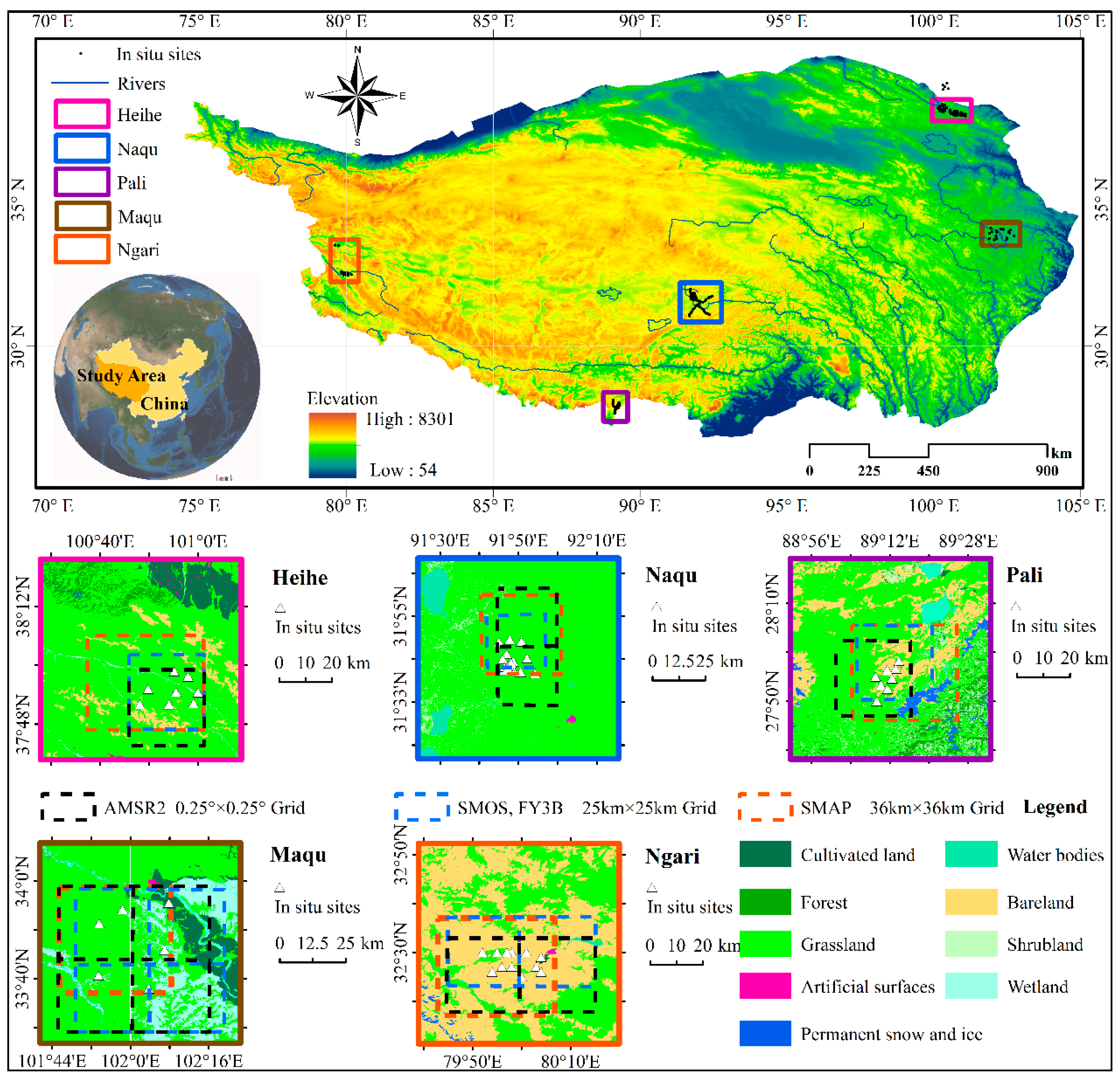
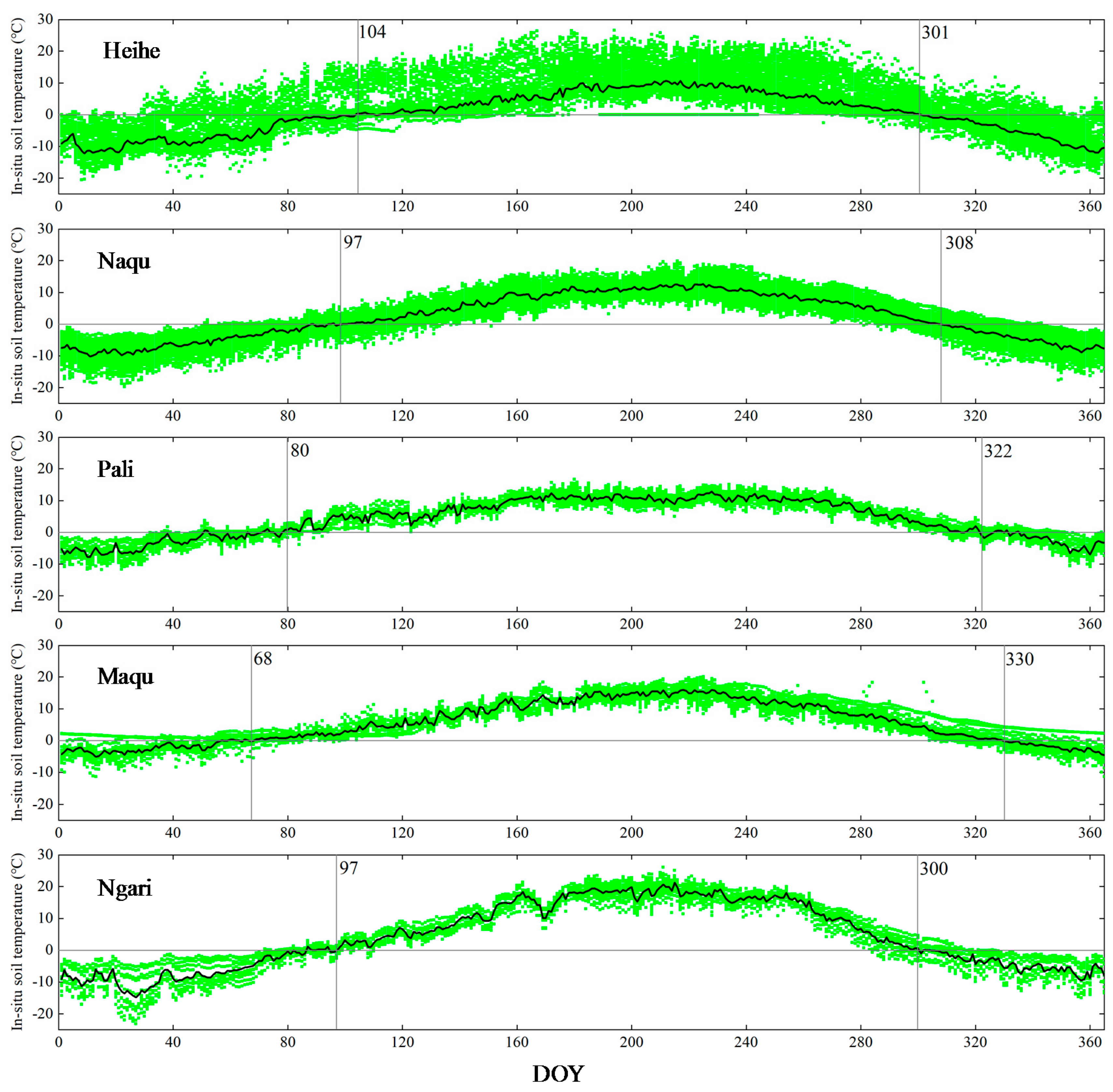
2.1. Study Area and In situ Measurements

The QTP (Figure 1) covers an area of more than 2.57 × 10⁶ km² in western China. The QTP has complex terrain and an average altitude of 4000 m above sea level. In recent decades, the QTP has experienced rapid hydroclimatic change [35]. This warming trend has occurred in most areas of the QTP and exhibits significant altitudinal dependence [36,37]. Compared to temperature changes, precipitation changes on the plateau are much more complex, and precipitation shows regional and seasonal differences [38,39]. All these reasons produce a complex SM situation in the QTP.

Table 1. Information of the in situ networks.

Networks	Heihe	Naqu	Pali	Maqu	Ngari
Location over the QTP	Northeast	Central	South	East	West
Selected/Total Nodes	8/40	16/56	8/25	7/20	12/18
Measured Depth	4 cm	0–5 cm	5 cm	5 cm	5 cm
Measured Interval	5 min	30 min	30 min	15 min	15 min
Time Coverage	07/2013–12/2015	07/2012–09/2016	07/2013–12/2015	06/2015–09/2016	07/2012–09/2016
Average Elevation*	3423 m	4866 m	4742 m	3711 m	4869 m
Average NDVI*	0.28	0.29	0.21	0.45	0.09
Land cover*	Grassland	Grassland	Grassland	Grassland, Wetland	Bare land, Grassland
Soil Texture (clay)*	18%	16%	15%	21%	11%
Soil Texture (sand)*	54%	63%	64%	45%	75%
Topography*	Mountainous	Flat	Flat	Hilly	Flat

* The average NDVI, which was calculated between Apr and Sep from 2015 to 2018, and the elevation, land cover, soil texture, etc., are introduced in Section 2.3.

summarizes the main characteristics of the five in situ networks (i.e., Heihe, Naqu, Pali, Maqu, and Ngari) in this study. The Heihe network’s (magenta rectangle in Figure 1) dataset is from WATER-NET [40,41,42,43,44,45], the Naqu (blue rectangle in Figure 1) and Pali (purple rectangle in Figure 1) networks’ datasets are acquired from CTP-SMTMN [46], and the Maqu (brown rectangle in Figure 1) and Ngari (orange rectangle in Figure 1) networks’ datasets come from Tibet-Obs [20,21].

2.2. Satellite-Based Soil Moisture Products

In this study, five satellite remotely sensed SM products were collected, including SMAP, SMOS-IC, FY3B, JAXA, and LPRM.

Table 2. Information of the five satellite-based soil moisture (SM) products.

SM Datasets	SMAP	SMOS-IC	FY3B	JAXA	LPRM
Incidence angle (°)	40	0–55	45	55	55
Frequency (GHz)	1.41	1.4	10.7, 18.7	10.7, 36.5	10.7, 36.5
Spatial Resolution	36 km	25 km	25 km	0.25°	0.25°
Temporal Coverage	2015–present	2010–present	2011–present	2012–present	2012–present
Ascending	18:00	6:00	13:40	13:30	13:30
Descending	6:00	18:00	1:40	1:30	1:30

lists the spatial resolutions and important basic information of the five SM datasets. The SMAP SM product [47] that was used in this study was the level-3 daily SM product (version 4.00), which was downloaded from https://nsidc.org/data/spl3smp/versions/4/. The SMOS-IC SM product (version 105) [16] is available at https://www.catds.fr/Products/Available-products-from-CEC-SM/SMOS-IC. FY3B is a second-generation polar orbiting meteorological satellite from China that was launched in November 2010. The FY3B MWRI SM product [12] was obtained from http://satellite.nsmc.org.cn/PortalSite/Data/Satellite.aspx. Both the JAXA [14] and LPRM [15] SM products come from the AMSR2 sensor of the GCOM-W1 mission, which was launched in May 2012. The JAXA level-3 product is available at https://gportal.jaxa.jp/gpr/information/download, and the LPRM level-3 (version 3.00) dataset come from https://search.earthdata.nasa.gov/.

The SM retrieval of FY3B was not performed in frozen soil or snow [12]. Moreover, other SM products have high uncertainties in frozen seasons because of the limited applicability and accuracy of the adopted dielectric constant models under frozen soil conditions; in frozen seasons, their SM products are difficult to use in most applications. However, the SMOS-IC and SMAP products provide flag values that can indicate frozen or snow-covered ground, which provides great convenience for product users. Therefore, in this study, the evaluation of the five passive microwave SM products was conducted only during the thawed seasons. In addition, except for the SMOS-IC and SMAP, all data of other three SM products were used in this study. For SMOS-IC, the data was filtered by the quality flags (0: Data OK, 1: Retrieve successfully but not recommended, 2: Missing data). Due to the strict control of data quality by SMOS-IC, the amount of data filtered by the flag 0 was extremely low over the QTP. To evaluate as much SMOS-IC SM data as possible and ensure its practicality, the data with quality flag 0/1 was used in this study. For SMAP, the data ranged from 0.02 to 0.5 cm³cm⁻³ is used in this study.

2.3. Geographical Configuration Data

For a comprehensive comparison, analysis, and evaluation of the performance of the five SM products, geographical and environmental auxiliary data were also collected in the study area. The auxiliary data included high-resolution map of Earth’s land cover (GlobeLand30) [48], the Global 30 Arc-Second Elevation (GTOPO30) [49], a precipitation dataset (CN05.1) [50], and a soil texture dataset comes from the Data Center for Resources and Environmental Sciences, Chinese Academy of Sciences (RESDC). MODIS/Terra normalized difference vegetation index products (NDVI, including MOD13C1 and MYD13C1) and the land-surface temperature (LST, MOD11C1) were also used. The GlobeLand30 dataset was downloaded from http://www.globallandcover.com/GLC30Download/. The GTOPO30 data were downloaded from https://lta.cr.usgs.gov/GTOPO30. The CN05.1 dataset was obtained from http://data.cma.cn/. The soil texture dataset was provided by http://www.resdc.cn. Both the NDVI and LST products were downloaded from https://search.earthdata.nasa.gov/search.

2.4. Methods

2.4.1. Data Preprocessing

Data preprocessing is required for both spatiotemporal in situ and satellite-based datasets for accurate data evaluation. To ensure the temporal consistency between the in situ and satellite data, the in situ values were averaged over 2-h windows before and after the corresponding equatorial overpass time, and these values were used for comparison with satellite-based data (similar processing can also be found in some previous works, e.g., References [9,51,52,53]). As mentioned in Section 2.2, the evaluation was conducted only in the unfrozen season.

In the direct validation, the values from the original grids of the five satellite-based products were used for comparison with in situ datasets during the unfrozen seasons. To determine these unfrozen seasons, a discriminating method for frozen vs. thawed seasons [54] was utilized in this work. As shown in Figure 2, this method provided the annual mean in situ soil temperature of each network. For each in situ network, the unfrozen seasons included the number of days that the in situ soil temperature was greater than 0 °C.

In the indirect validation, a nearest-neighbor sampling approach (e.g., References [55,56]) was used to re-project all the satellite-based products (including SMAP, SMOS-IC, FY3B, and NDVI) into regular 0.25°×0.25° grids. A fixed period from April to September was defined as the unfrozen season according to some previous works (e.g., References [21,22]). To utilize more SMAP datasets, the time range of the datasets in the indirect validation spanned from April 2015 to July 2018, which was different from the time range in the direct validation.

2.4.2. Performance Index

In this study, three statistical indices were used to evaluate the accuracy of the five time-series SM products [57]:

$$\mathrm{R}=\mathrm{E}\left[\left(\mathrm{S}{\mathrm{M}}_{\mathrm{e}\mathrm{s}\mathrm{t}}-\mathrm{E}\left[\mathrm{S}{\mathrm{M}}_{\mathrm{e}\mathrm{s}\mathrm{t}}\right]\right)\left(\mathrm{S}{\mathrm{M}}_{\mathrm{r}\mathrm{e}\mathrm{f}}-\mathrm{E}\left[\mathrm{S}{\mathrm{M}}_{\mathrm{r}\mathrm{e}\mathrm{f}}\right]\right)\right]/({\mathsf{\sigma }}_{\mathrm{e}\mathrm{s}\mathrm{t}}\times {\mathsf{\sigma }}_{\mathrm{r}\mathrm{e}\mathrm{f}})$$

(1)

$$\mathrm{R}\mathrm{M}\mathrm{S}\mathrm{E}=\sqrt{\mathrm{E}[{(\mathrm{S}{\mathrm{M}}_{\mathrm{e}\mathrm{s}\mathrm{t}}-\mathrm{S}{\mathrm{M}}_{\mathrm{r}\mathrm{e}\mathrm{f}})}^2]}$$

(2)

$$\mathrm{B}\mathrm{i}\mathrm{a}\mathrm{s}=\mathrm{E}\left[\mathrm{S}{\mathrm{M}}_{\mathrm{e}\mathrm{s}\mathrm{t}}\left]-\mathrm{E}\right[\mathrm{S}{\mathrm{M}}_{\mathrm{r}\mathrm{e}\mathrm{f}}\right]$$

(3)

where SM_est is the satellite-derived soil moisture, SM_ref is the in situ soil moisture, E represents the expected value, σ stands for the standard deviation operation, R is the Pearson correlation coefficient, RMSE is the root mean square error (unit: cm³ cm⁻³), and Bias is the mean difference (unit: cm³ cm⁻³) between the satellite SM_est products and the in situ SM_ref. These indices are not calculated unless the SM samples (N in

Table 3. Performance metrics of the SMAP, SMOS-IC, FY3B, JAXA, and LPRM soil moisture data products for the unfrozen seasons from 2012 to 2016 in the five validation networks *.

In situ Networks	Product	SMOS-IC Ascending; SMAP, AMSR2, and FY3B Descending (morning orbits)				SMOS-IC Descending; SMAP, AMSR2, and FY3B Ascending (afternoon orbits)
		R	RMSE	Bias	N	R	RMSE	Bias	N
Heihe Network	SMAP	0.779	0.105	−0.104	91	0.643	0.113	−0.110	78
	SMOS-IC	0.302	0.143	−0.115	172	0.177	0.115	−0.041	157
	FY3B	−0.042	0.119	−0.013	106	0.330	0.152	−0.120	262
	JAXA	0.357	0.284	−0.277	404	0.389	0.279	−0.275	387
	LPRM	0.305	0.249	0.199	371	0.168	0.167	0.106	381
Naqu Network	SMAP	0.816	0.066	−0.019	142	0.835	0.078	−0.002	140
	SMOS-IC	0.472	0.141	−0.049	222	0.428	0.182	−0.130	191
	FY3B	0.750	0.116	0.072	78	0.755	0.109	0.026	456
	JAXA	0.718	0.168	−0.087	686	0.808	0.146	−0.061	677
	LPRM	0.768	0.113	0.090	632	0.798	0.064	0.041	669
Pali Network	SMAP	0.615	0.057	−0.045	143	0.672	0.046	−0.034	95
	SMOS-IC	0.524	0.090	−0.026	87	0.604	0.073	−0.060	110
	FY3B	-	-	-	0	0.292	0.055	−0.040	137
	JAXA	0.527	0.087	−0.080	234	0.541	0.087	−0.081	235
	LPRM	0.538	0.220	0.212	200	0.339	0.169	0.161	235
Maqu Network	SMAP	0.814	0.076	−0.066	123	0.721	0.088	−0.072	108
	SMOS-IC	0.638	0.112	−0.074	334	0.485	0.083	−0.008	339
	FY3B	0.529	0.137	−0.026	187	0.486	0.136	−0.072	509
	JAXA	0.420	0.292	−0.282	747	0.540	0.228	−0.214	744
	LPRM	0.419	0.099	0.042	734	0.031	0.120	0.001	743
Ngari Network	SMAP	0.335	0.054	−0.047	109	0.567	0.045	−0.041	131
	SMOS-IC	0.097	0.120	0.003	267	0.116	0.092	−0.022	263
	FY3B	-	-	-	0	0.175	0.040	−0.029	380
	JAXA	0.398	0.060	−0.055	619	0.364	0.062	−0.056	608
	LPRM	0.418	0.124	0.111	321	−0.208	0.117	0.111	597

* The darker the color, the larger the statistical value is.

) are more than 30.

2.4.3. Three-Cornered Hat (TCH) Method

The performance of the traditional TCH method in estimating uncertainty results (the uncertainty, which can be used to reflect the estimate errors of various time-series products) largely depends on two major assumptions: ‘zero error cross-correlation’ and ‘error orthogonality’ [28]. ‘Zero error cross-correlation’ requires the mutual independence of errors of various time series, and ‘error orthogonality’ requires independency between the errors and unknown true values. Moreover, the effect of ‘zero error cross-correlation’ on the estimated results is greater than that of ‘error orthogonality’ [28,58,59]. Both of these assumptions limit the application of the TCH method, especially when processing time-series data that are statistically dependent on each other. Currently, the improved TCH method can overcome these limitations and considers the correlations among the corresponding noise sequences of multiple time series (more than three) by minimizing any global correlations. In the absence of a reference SM dataset, the TCH method is algebraically simply applied to estimate the uncertainties of each SM product [28,29,60]. In this study, this method was employed to estimate the uncertainties of five passive microwave remotely sensed SM products (i.e., SMAP, SMOS-IC, FY3B, JAXA, and LPRM) without any prior knowledge. The detailed computational procedure of the improved TCH method is given in Appendix A.

3. Results

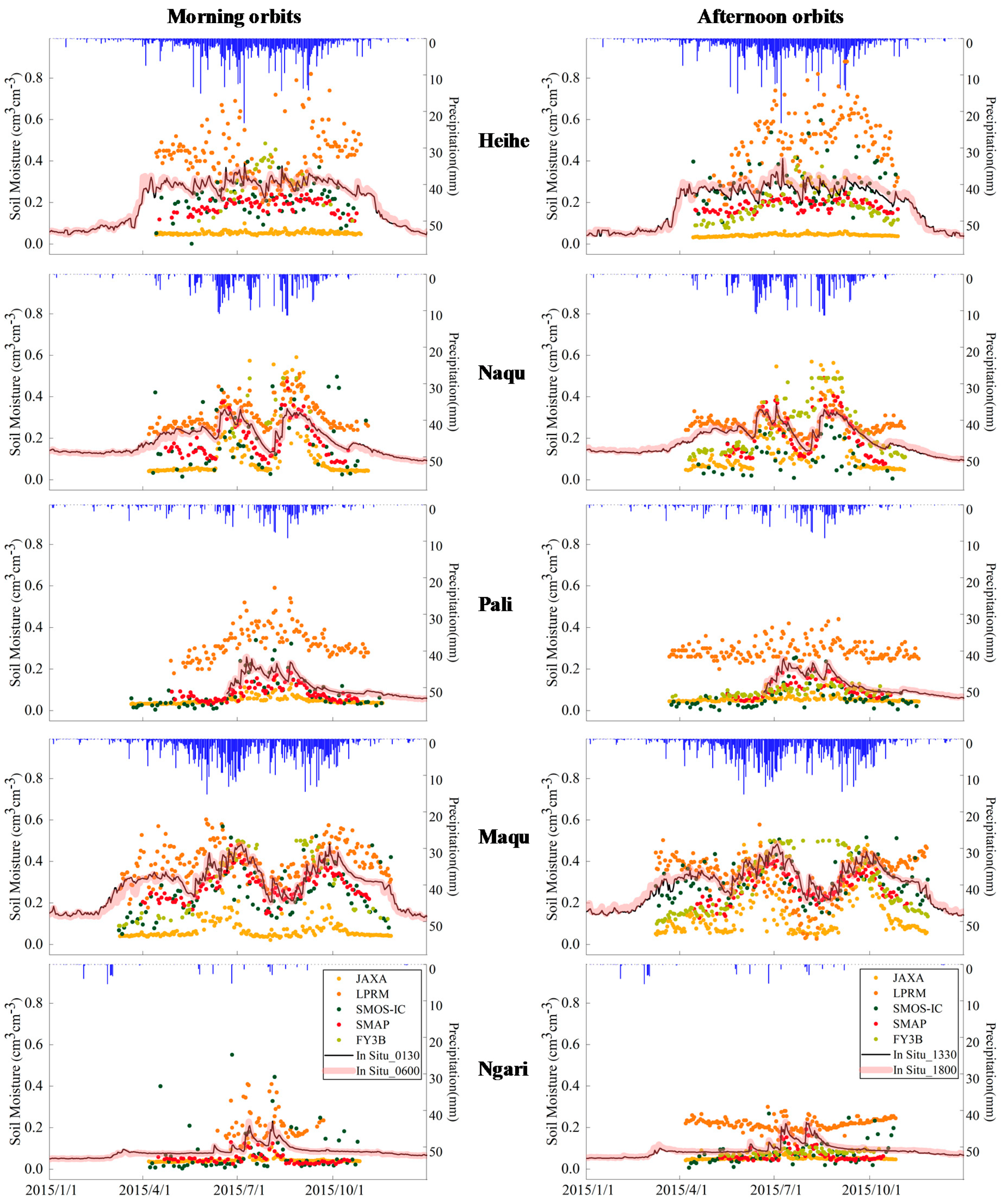
3.1. Direct Comparison of Time Series

From a temporal perspective, the accuracy of the satellite-based SM data was assessed by comparisons with the in situ SM at five networks. The temporal comparisons in 2015 are illustrated in Figure 3, and the temporal comparison results from 2012 to 2016 are presented in the supplementary information. Referring to the precipitation data, the in situ measurements captured the precipitation events and soil moisture’s temporal trends in each in situ network. Corresponding changes in the five SM products during precipitation events are shown in Figure 3. The detailed performances of the temporal variations and the accuracy indices for each SM product for each in situ network are introduced below.

In the Heihe network, the SM was severely overestimated by the LPRM ascending and descending products and underestimated by the JAXA. Table 3 shows the extremely high bias values for the LPRM (0.20 cm³ cm⁻³ for the descending orbit, 0.11 cm³ cm⁻³ for the ascending orbit) and the extremely low bias values for the JAXA (−0.28 cm³ cm⁻³ for the descending orbit, −0.27 cm³ cm⁻³ for the ascending orbit). For SMOS-IC and FY3B, noisy performances of capturing temporal variations could be found, while FY3B had relatively good dynamics in the afternoon orbit, and SMOS-IC had relatively better correlations with the in situ measurements in the morning orbit. Moreover, the SMOS-IC is close to SMAP in the magnitude of time series, especially in their morning orbits. The SM was slightly underestimated by both the ascending and descending SMAP products, but SMAP had high consistency with the in situ observations (R values of 0.78 for the descending orbit and 0.64 for the ascending orbit).

In the Naqu network, the SM was slightly underestimated by the descending SMAP with a bias of −0.02 cm³ cm⁻³ and an RMSE of 0.066 cm³ cm⁻³. The ascending SMAP had a bias approaching zero and an RMSE of 0.078 cm³ cm⁻³ (Table 3). Similar to SMAP, the temporal variations in the other four SM products were compared to the in situ SM (Figure 3), which had relatively higher R values. In addition, the SM was slightly underestimated by SMOS-IC and the JAXA and overestimated by FY3B and the LPRM. Except for SMAP and SMOS-IC, the products had better accuracy in their afternoon orbits.

In the Pali network, the SM was seriously overestimated by the LPRM descending product, with a bias of 0.21 cm³ cm⁻³ and an RMSE of 0.22 cm³ cm⁻³, and the ascending product had a bias of 0.16 cm³ cm⁻³ and an RMSE of 0.169 cm³ cm⁻³. FY3B had modest accuracy in its ascending orbit, with a bias of −0.04 cm³ cm⁻³ and an RMSE of 0.055 cm³ cm⁻³. The temporal variations in SM could be well fitted by the SMAP, SMOS-IC, and JAXA products. SMAP and SMOS-IC had more modest accuracy than the JAXA in their afternoon orbits.

In the Maqu network, the SMAP ascending and descending products performed best, with relatively high R values and relatively low bias and RMSE values. In the morning orbits, the SM was slightly overestimated by the LPRM and underestimated by other four products to varying degrees. In addition, the LPRM showed the opposite trend in the afternoon orbits, and SMOS-IC had the best absolute accuracy (RMSE: 0.083 cm³ cm⁻³) in the afternoon orbit.

In the Ngari network, the SMAP ascending and descending products had relatively low bias and RMSE values, which were close to the official target accuracy. Compared to other four SM products, SMAP was more consistent with the in situ measurements. Except for the LPRM, the SM was slightly underestimated by other four products (i.e., SMAP, SMOS-IC, FY3B, and JAXA), with relatively low bias and RMSE values, especially in their afternoon orbits.

The negative correlation between morning-orbit FY3B SM product and in situ measurements only appeared in the Heihe network, and the negative correlation between afternoon-orbit LPRM SM product and in situ measurements occurred in the Ngari network. For FY3B, the R value is near zero, and the negative correlation may be caused by the sample size (the amount of valid sample of FY3B is low and these data are clustered in the summer season). For LPRM, the overall performances in its afternoon orbit were worse than in its morning orbit, even the negative correlation that appeared in the Ngari network, which was caused by the poor estimates of soil moisture in the seasons except for summer season. As shown in the Figure 3, the obviously opposite seasonal trend was found in Ngari networks. In summary, compared to other four SM products (i.e., SMOS-IC, FY3B, JAXA, LPRM), SMAP was more consistent with in situ SM (its overall R in five in situ networks is 0.680, RMSE is 0.073 cm³ cm⁻³, and Bias is −0.054 cm³ cm⁻³), especially in the relatively sparse vegetation areas (i.e., the Ngari network) and relatively dense vegetation areas (i.e., the Maqu network). Moreover, SMAP achieved or was close to its target accuracy in many networks (i.e., the Naqu, Pali, Maqu, and Ngari networks). For all SM products, good consistency between satellite-based and in situ measurements was found in the Naqu network, with high R values (the overall R for five products is 0.715). The overestimation by LPRM (the overall R: 0.358, RMSE: 0.144 cm³ cm⁻³, Bias: 0.107 cm³ cm⁻³), the underestimation by JAXA (the overall R: 0.506, RMSE: 0.169 cm³ cm⁻³, Bias: −0.147 cm³ cm⁻³) and SMOS-IC (the overall R: 0.384, RMSE: 0.115 cm³ cm⁻³, Bias: −0.052 cm³ cm⁻³), the slightly noisy dynamics of SMOS-IC, and the good seasonality but poor absolute accuracy of FY3B (the overall R: 0.409, RMSE: 0.108 cm³ cm⁻³, Bias: −0.025 cm³ cm⁻³) were all reflected in most of the in situ networks.

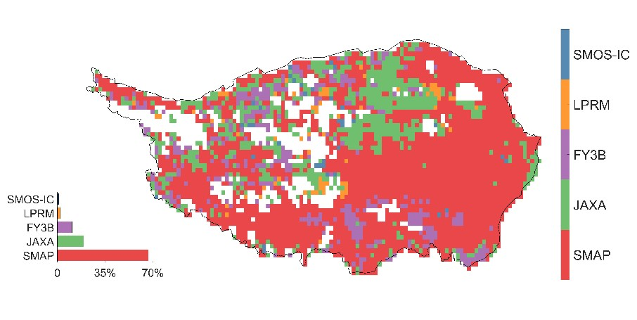
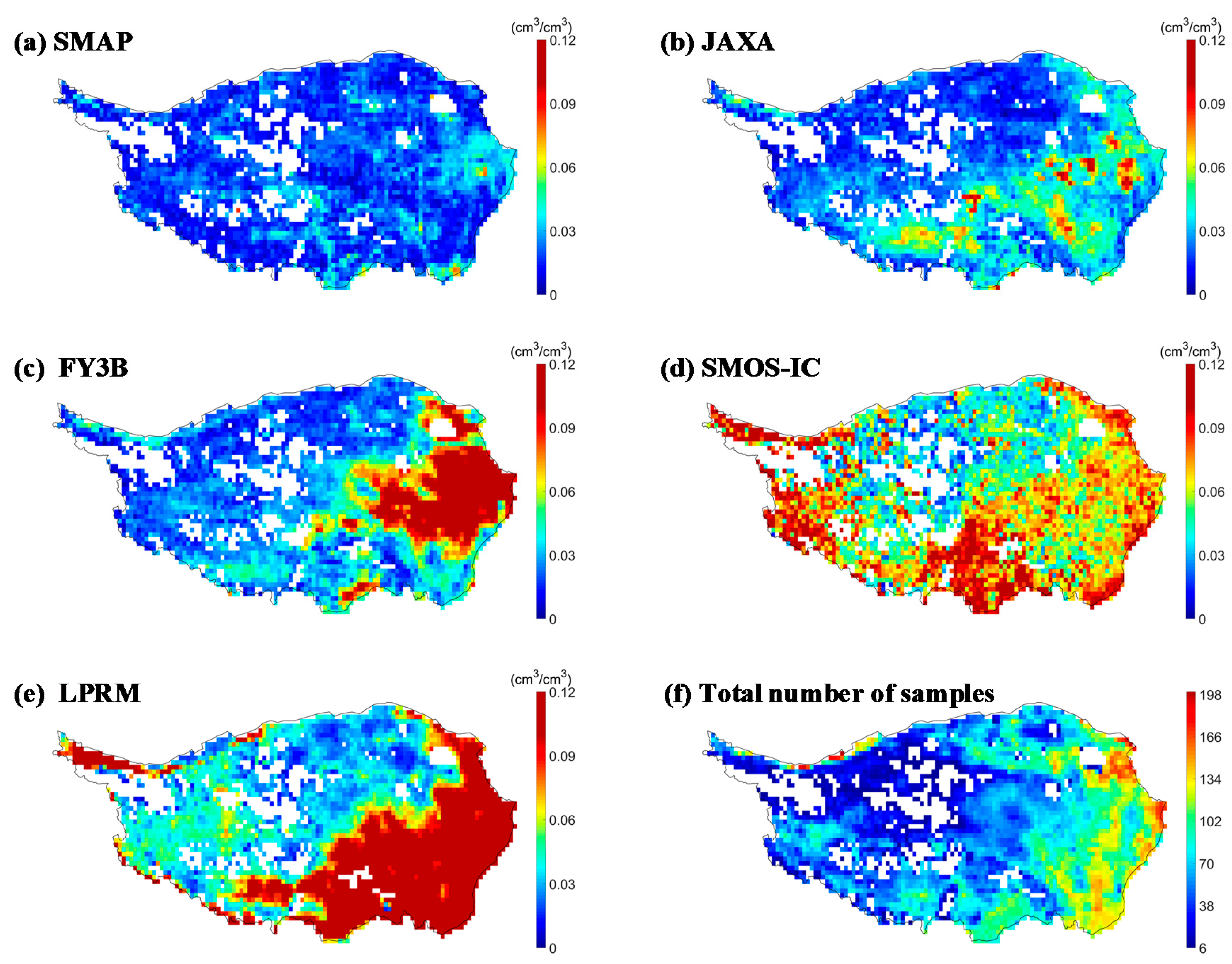
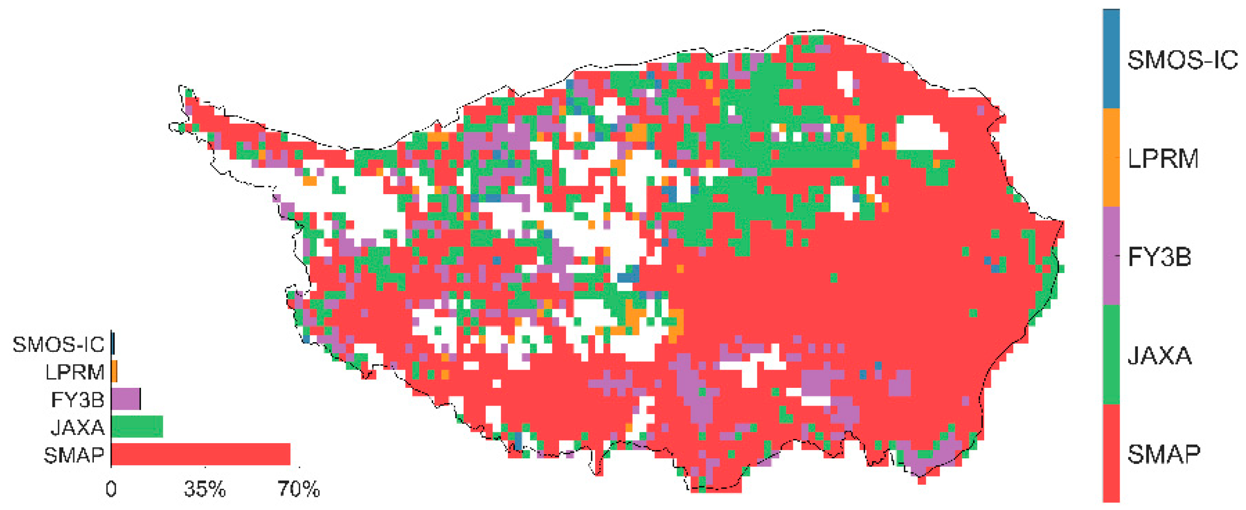
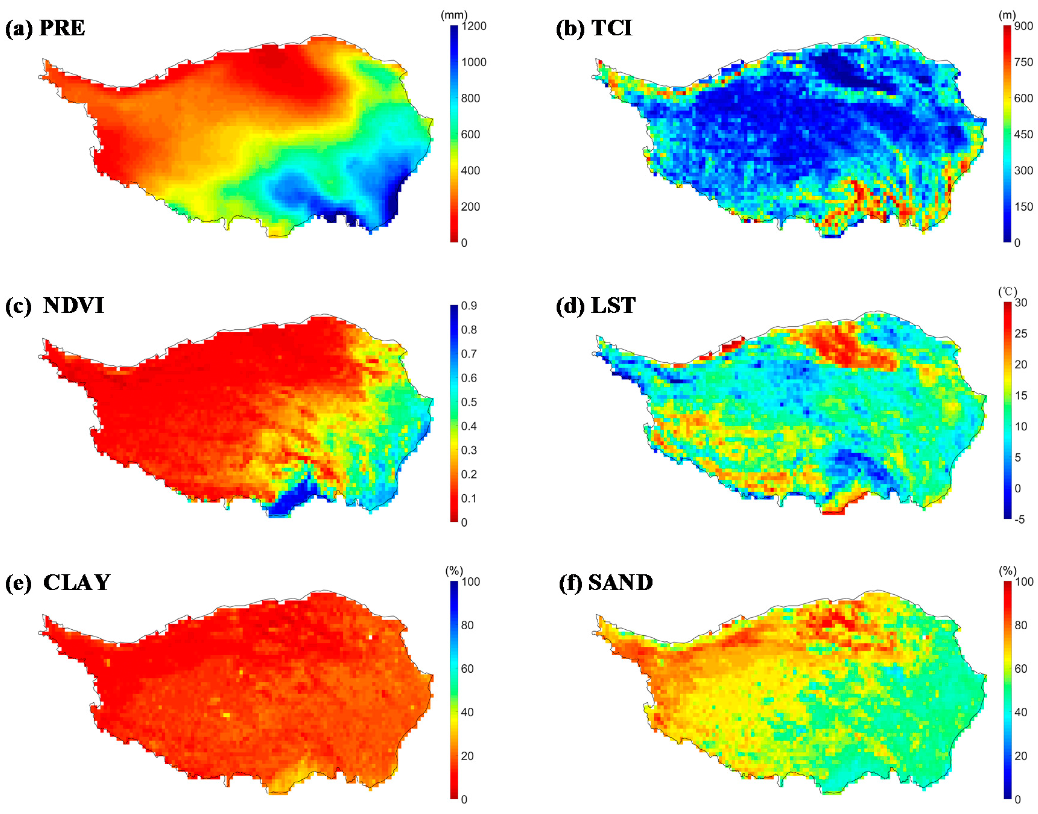
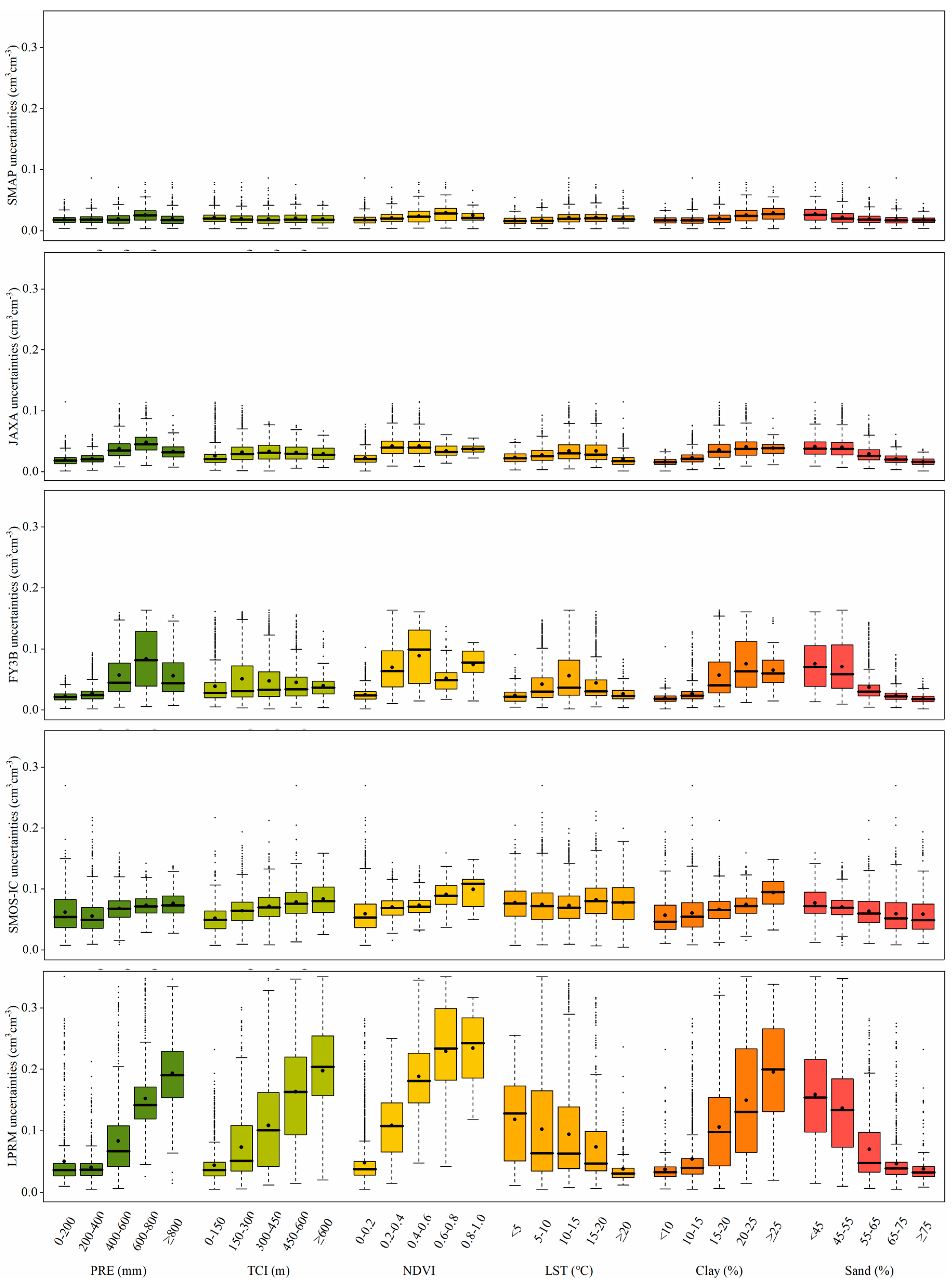
3.2. Indirect Comparisons of the Spatial Distribution

The uncertainty maps over the QTP for the five remotely sensed SM products were derived by using the TCH method (Figure 4). The time coverage between the spatial comparison and time-series comparison was not completely consistent. Only the SM products within the unfrozen seasons (i.e., from April to September) from April 2015 to July 2018 were used in this section. In addition, the daily values of each SM product in this section were the average of the ascending and descending SM estimates.

The TCH-based evaluation showed that the spatial patterns of the uncertainties for the five SM products are varied a lot. SMAP had low uncertainties over the entire QTP, and SMOS-IC presented relatively high uncertainties, overall. The other three SM products (JAXA, FY3B, and LPRM) showed relatively low uncertainties in the mid-western QTP but relatively high uncertainties in the mid-eastern QTP. The regional mean uncertainty of SMAP was 0.020 cm³ cm⁻³, the lowest value compared to those of other SM products. The JAXA also had a relatively low mean uncertainty of 0.029 cm³ cm⁻³, which was close to that of SMAP. The regional mean uncertainties of FY3B and SMOS-IC were relatively high, i.e., 0.043 cm³ cm⁻³ and 0.071 cm³ cm⁻³, respectively. In addition, the LPRM, which had a regional mean uncertainty of 0.098 cm³ cm⁻³, had exceptionally high uncertainties in the eastern QTP. The more samples that participated in the TCH process, the more stable and reliable the uncertainty results became [31]. Generally, the model could be run when the number of samples was greater than the number of SM products (five in this study) that participated in the TCH process. The larger the number of samples, the more robust the TCH results became. Figure 4f shows the total number of samples that were used on each pixel in this experiment. Because of the large amount of missing values for SMOS-IC and FY3B, the number of common observations for the eastern QTP was much larger than that for the mid-western QTP, with many blank areas present over the QTP.

Figure 5 shows the areas where SMAP (in dark-red pixels) presented the lowest uncertainty among the five SM products; the number of SMAP pixels comprised 66.64% of the total pixels. Meanwhile, the JAXA comprised 19.39%, FY3B comprised 10.83%, LPRM comprised 2.11%, and SMOS-IC comprised 1.03%. In fact, based on empirical research from Awange et al. [31], the reference is immaterial because the same uncertainty results can be obtained regardless of the chosen reference. In this study, SMAP was selected as the reference SM. SMAP presented the smallest uncertainties in the eastern QTP, which received a relatively high amount of precipitation (see Figure 6) and had a high temporal variability of SM (in the Heihe, Maqu, and Naqu areas), and showed the smallest uncertainties in most areas of the western QTP, which was relatively arid with a low dynamic SM change. On the other hand, the lowest uncertainties were obtained from the LPRM, JAXA, and FY3B in the mid-western QTP, which had low to moderate precipitation and a low temporal variability of SM (in the Ngari area).

The primary causes of the varying spatial patterns of the uncertainties included the diverse environmental conditions and the different inputs and parameterization schemes of the SM retrieval algorithms. The related variables mainly included the precipitation, terrain complexity, vegetation, land-surface temperature, and soil texture. To better explain the spatial behavior of the uncertainty, it was viewed against some climatic and environmental variables (Figure 6), including the annual precipitation (PRE), terrain complexity index (TCI, represented by the standard deviation of 30″ DEM within 0.25° pixels.), NDVI, LST, and soil texture (percentage of clay and sand). These variables were calculated during the same period as that of the TCH estimates. Overall, the uncertainties of SMAP and the JAXA were relatively low, both of which changed slightly as these selected variables changed. SMOS-IC was unaffected by these variables, and this product’s uncertainty showed great randomness throughout the QTP. FY3B and LPRM were greatly affected by these selected factors, and the relationships between the uncertainty and selected variables were similar between these two SM products.

As a main driving factor, precipitation determines the magnitude and spatial pattern of SM. By comparing the PRE map (Figure 6) with the TCH results (Figure 4), the three SM products (JAXA, FY3B, and LPRM) performed worse in relatively humid areas than in arid regions, and their uncertainty maps showed a similar spatial pattern to that of the PRE map. According to Figure 6 and Figure 7, the TCI was relatively large in the periphery of the QTP but relatively low in the mid-western QTP. Similarly, the LPRM showed larger uncertainties when the TCI was larger. Meanwhile, the JAXA and FY3B were slightly affected by the TCI, and the five SM products showed low uncertainties in flat areas. The NDVI showed an increasing trend from the northeastern to southeastern QTP, and the uncertainties of FY3B and the LPRM showed a similar trend with that of the NDVI. All the SM products were affected by NDVI to a certain degree: The larger the NDVI, the larger the uncertainties became. Obviously, most of the SM retrieval algorithms may not have affected the removal of vegetation factors in the retrieval results. As another important input of SM retrieval algorithms, the relationship between the LST and SM uncertainties seemed to have not been analyzed here, especially for SMAP and SMOS-IC. In addition, the spatial patterns of the percentage of clay and sand showed the opposite trend. Most of the SM products performed worse in areas with higher sand content or lower clay content. The percentage of clay/sand is strongly related to PRE, so the relationship between the SM uncertainties and soil texture may have been affected by PRE and may not always reflect the effects of the soil texture on the SM retrieval results.

4. Discussions

The evaluation of passive microwave remotely sensed SM products is an important and challenging task. In the direct validation, the in situ measurements can only be considered as a close approximation and not a ‘true value’ of soil moisture at the pixel scale, which brings great uncertainties to the results of direct comparison. In the indirect validation, the disparities in sensing depths, spatial resolutions, retrieval algorithms and inputs, etc., contribute to the difficulties of inter-comparing different soil moisture products. The factors that produced uncertainty when validating five SM products included these points: (i) The difference between the measured depths of SM from different sources (including different sensing depths from the different frequencies of the sensors and different measurement depths from the different in situ probes) [61]; (ii) the mismatch in spatial scales between in situ and satellite-based measurements and the disparity in spatial resolutions between different SM products [62]; (iii) the different retrieval algorithms and corresponding inputs of different SM products [17]; and (iv) the errors from in situ and satellite-based sensors.

The possible errors in the evaluation results that were caused by different sensing depths must be considered carefully, when validating multiple sensor-based products on multiple in situ observation networks. As shown in Table 1, the sensor on each in situ node was inserted into ~5-cm topsoil, which more closely matches the sensing depth of L-band passive microwave sensors (i.e., SMAP and SMOS). In the direct comparison (Section 3.1), the L-band SM products (i.e., SMAP and SMOS) should have performed better than the X-band products (i.e., FY3B, JAXA, and LPRM), especially in terms of the magnitudes of the time series. Moreover, a good correlation should have existed between the L-band and X-band measurements because the land cover type of the QTP is dominated by bare land and grassland. Therefore, the different sensing depths, which were caused by the disparity in the sensing depths, barely affected the magnitude of the calculated R values in the direct comparison. However, as an L-band product, SMOS-IC (overall R of 0.384 compared to the in situ measurements) was not more reliable than other X-band products (i.e., FY3B and the JAXA, with overall R values of 0.409 and 0.506, respectively) in the time series. Moreover, as an X-band product, the JAXA (overall Bias value of −0.025 cm³cm⁻³) had the lowest bias of all the products. Obviously, these performances could not have been caused by only the different sensing depths.

Another key issue when validating SM products is the mismatch in spatial scales between in situ and satellite observations [9]. Conventional in situ measurements of SM are conducted at a point, but satellite-based sensors observe an integrated area value for a larger spatial extent. As mentioned in Table 2, the five SM products in this study provided their datasets at ~25-km (SMOS-IC, FY3B, JAXA, and LPRM) or 36-km (SMAP) resolution. Therefore, the errors in the evaluation work from any mismatch in the spatial scales, cannot be neglected, and some efforts must be taken to weaken its effect. This study did take measures to weaken these errors, but possible errors must still be considered when referring to this work. These efforts are mainly reflected in the preprocessing work of the direct and indirect comparisons. In the direct comparison, the SM products with original spatial resolutions were used for comparison with the in situ measurements to maintain fairness between the various SM products. The upscaling work for the in situ measurements was based on the arithmetic averaging method, which is relatively simple and reliable (e.g., References [9,21,22,24,52,53,63]). In the indirect comparison, the spatial scale had to be resampled to compare the five products for each pixel (e.g., References [59,64,65]). Of course, reprocessing these datasets introduced some errors into the results. Therefore, the TCH-based results were only analyzed in terms of their spatial patterns (Figure 4) and statistical performances (Figure 5 and Figure 7) to decrease the uncertainty.

In addition, the errors from retrieval algorithms and their inputs play an important role in the performance of SM products [9]. The baseline algorithms of SMAP, SMOS-IC, FY3B, the JAXA, and the LPRM are single-channel algorithms that are based on TB_V measurements (SCA-V) [47], L-band microwave emission of the biosphere (L-MEB) [17], dual-channel soil moisture retrieval algorithm [12], look-up table [14], and land parameter retrieval model (LPRM) [15], respectively, which are all based on the τ-ω model [66]. In this model, which ignores atmospheric effects, served brightness temperature TB^p under polarization p (p=V/H) can be expressed as

$$\mathrm{T}{\mathrm{B}}^{\mathrm{p}}=\left(1-{\mathsf{\omega }}^{\mathrm{p}}\right)\left(1-{\mathsf{\gamma }}^{\mathrm{p}}\right){\mathrm{T}}_{\mathrm{C}}+\left(1-{\mathsf{\omega }}^{\mathrm{p}}\right)\left(1-{\mathsf{\gamma }}^{\mathrm{p}}\right){\mathsf{\gamma }}^{\mathrm{p}}\left(1-{\mathsf{\epsilon }}_{\mathrm{g}}^{\mathrm{p}}\right){\mathrm{T}}_{\mathrm{C}}+{\mathsf{\epsilon }}_{\mathrm{g}}^{\mathrm{p}}{\mathsf{\gamma }}^{\mathrm{p}}{\mathrm{T}}_{\mathrm{G}}$$

(4)

where τ is the vegetation optical depth, ω is the equivalent scattering albedo, γ^p = exp (−τ^p/cosθ) is the vegetation transmissivity at an incident angle of θ, T_C is the effective vegetation temperature, T_G is the soil effective temperature, and ε_g^p is the rough surface emissivity.

Table 4. Main components of the SM operational algorithms of SMAP, SMOS-IC, JAXA, LPRM, and FY3B*.

Components	L3 SMAP	SMOS-IC	L3 JAXA	L3 LPRM	FY3B
Radiative Transfer Model	τ-ω model	τ-ω model	τ-ω model	τ-ω model	τ-ω model
Soil temperature (Ts)	Ts= f(T0, T∞),T0, T∞ form layer 1 and 2 of GEOS-5	Ts= f(T0, T∞), T0, T∞ from layer 1 and 3 of ECMWF, respectively	Ts=293 K	Ts =0.688 TB36.5 GHz_V+101.126	Ts≈Tv
Vegetation temperature (Tv)	Tv=Ts, at 6:00 a.m.	Skin (Level 1, top 0–7 cm soil layer) temperature from ECMWF	Tv=Ts=293 K	Tv= Ts	Tv =1.11×TB36.5 GHz_V -15.2
Optical depth (τ)	τ=τNAD×f(θ, p); τNAD=b*VWC; b=f(IGBP), b=0 to 0.13; VWC=f(NDVI, IGBP), f is a nonlinear relationship	The τ is also retrieved in the SMOS-IC algorithm	τ=b*VWC; b is constants; VWC is retrieved using lookup table; fc=f(NDVI), f is a nonlinear relationship	τ=f (MPDI, k, θ, ω); MDPI=(TBV-TBH)/(TBV+TBH), k is the absolute value of the soil dielectric constant	τ=b×VWC/cosθ VWC=5.0×NDVI2 (NDVI>0.5) VWC=2.5×NDVI2 (NDVI≤0.5) b is determined by experiments and model simulation
Albedo (ω)	ω=f(IGBP), ω=0 to 0.12	ω=f(IGBP), ω=0.06 to 0.12	ω=0.06 to 0.063	ω=0.06	ω≈0
Soil roughness model	QHN model; NV=NH=2; Q=0; H=f(IGBP), H=0.16 to 0.83;	QHN model; NH=NV=-1 for low vegetation, NH=1 and NV=-1 for forest; Q=0; H=f(IGBP), mean H=0.02–0.30	Constants Q and H; Q= 0.189 to 0.344; H=0.680 to 0.873	Constants Q and H; Q=0.2; H=0.2	Qp model; Qv(f)=a(f)+b(f)×Qh(f) f is frequency, a and b are obtained from the AIEM simulated dataset
Soil dielectric mixing model	Mironov, 2009	Mironov, 2009	Dobson, 1985	Wang and Schmugge, 1980	--

* Q: Polarization mixing parameter; H: surface roughness dimensionless parameter; N_H/V: an integer used to parameterize the dependence of the roughness effects on incidence angle; T_∞: The deep soil moisture (50–100 cm); T₀: The surface soil moisture (0–5 cm); p: Polarization; b: Vegetation parameter; f_c: Fractional vegetation index.

lists the main components of the SM operational algorithms of SMAP, SMOS-IC, the JAXA, the LPRM, and FY3B. According to Table 4, the differences between the inputs, i.e., the soil and vegetation physical temperatures, the vegetation optical and albedo parameters, and the different adopted models for surface roughness and soil permittivity, were some of the main factors that caused the different performances of the five SM products.

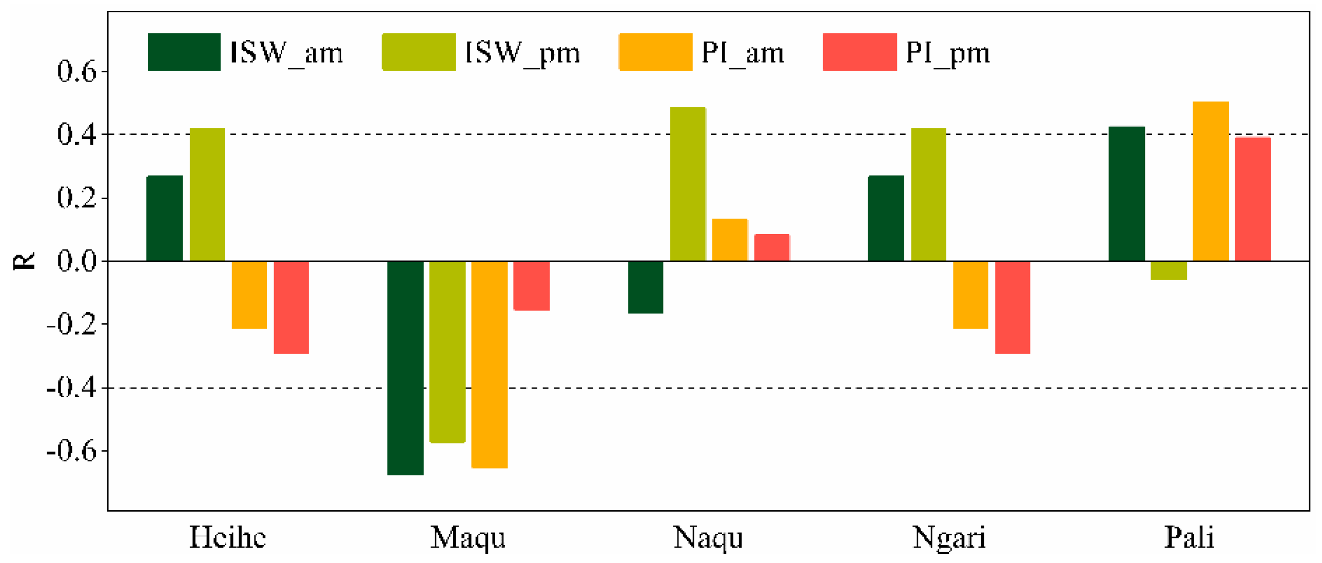
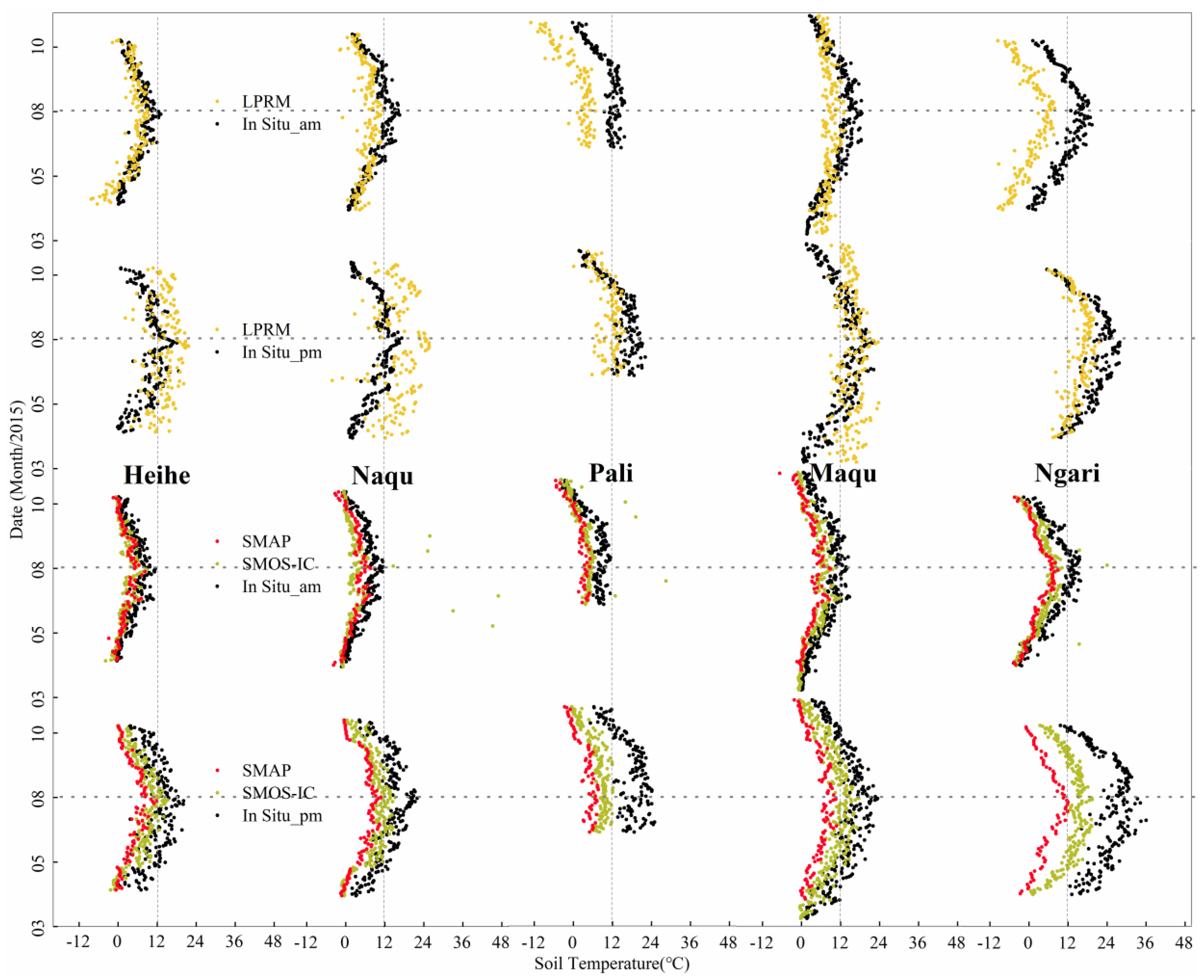
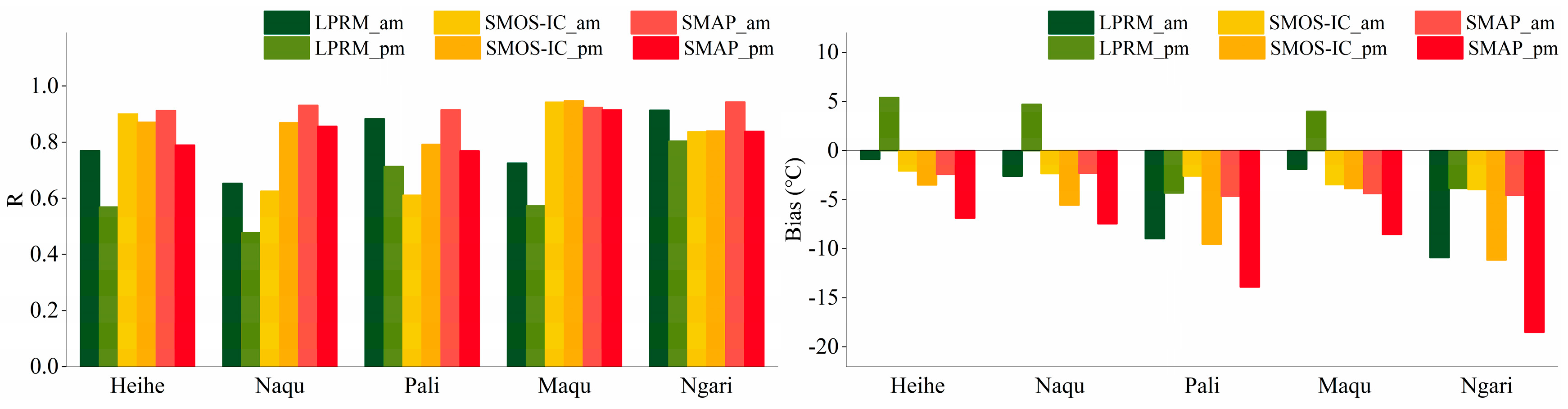
4.1. Land-Surface Temperature

The physical surface temperature is an important parameter for estimating SM and is the first parameter calculated in retrieval algorithms. As listed in Table 4, the estimations of the surface temperature varied widely in the five operational SM algorithms. The JAXA algorithm defined the soil temperature and vegetation temperature as constant under the assumption that the polarization index (PI) and index of soil wetness (ISW) could eliminate the effect of the physical surface temperature on SM retrieval [14]. However, according to the comparison results in Section 3.1, the JAXA SM often presented relatively small values in most regions. Specifically, with the exception of the Naqu network (located in a sub-humid area), the JAXA had a weak temporal variation and could not capture the main precipitation events, likely because the PI and ISW have limited ability to eliminate the surface temperature and because these two indices are still strongly related to T_s.

Figure 8 shows the correlation coefficients between the PI or ISW and the in situ T_s. Compared to Naqu, the other four in situ networks indicated a relatively stronger correlation between the PI/ISW and in situ T_s. Additionally, these two parameters seemed to barely eliminate the effect of the physical temperature of the land surface in most areas, which may explain why the JAXA had a wider range and more obvious dynamic variation in Naqu than in the other networks. Obviously, the correlation was weaker in relatively arid areas (e.g., Pali and Ngari) than in relatively humid regions (e.g., Heihe and Maqu), mainly because the JAXA calibrates its look-up table in Mongolia [14], which is an arid area. Therefore, the two indices can better characterize the surface temperature in relatively arid areas, while larger uncertainties occur in humid locations. Overall, the JAXA retrieval algorithm, which was based on look-up table, was less reliable, especially in relatively humid areas. Bindlish et al. [67] also found similar underestimations and limited value ranges of JAXA SM in many regions.

Figure 9 shows the comparison results between in situ T_s and satellite-derived T_s for the other three models. Both the LPRM and FY3B (T_S data were not available) estimate T_s based on an empirical relationship between T_s and V polarization TB [68,69] and have relatively good dynamic ranges, while SMOS-IC and SMAP obtain their physical surface temperature values from the ECMWF and GEOS-5 datasets, respectively [16,47]. The LPRM T_s exhibited better at nighttime than in daytime, and its overall R equaled 0.79 at nighttime and 0.61 in daytime (Figure 10). Moreover, with the exception of Pali and Ngari, overestimation occurred for the LPRM at the other networks during the day, mainly because the ascending and descending times were 1:30 pm and 1:30 am, respectively; these two time points roughly correspond to the highest and lowest temperatures of the day. In particular, the difference between canopy and soil temperature was relatively high at 1:30 pm, and the difference was relatively low at 1:30 am. Based on the results from Section 3.1, the LPRM performed better at nighttime compared to daytime, which may be explained by the fact that LPRM reasonably considers T_s=T_V at 1:30 am. For both SMOS-IC and SMAP, the estimated T_s had consistent performance in the five networks, and R was larger than 0.85 in most networks, which was slightly better at nighttime than in daytime. Notably, the T_s values of SMOS-IC and SMAP were underestimated to a certain degree. Generally, the soil temperature and soil dielectric properties are more uniform at 6:00 a.m. than at other times of the day [47]. Therefore, the use of T_v=T_s (the near surface soil temperature equals the canopy temperature) in the early morning should minimize SM retrieval errors. Slightly better performances were also found at nighttime (morning orbit) for the SMAP SM in most of the in situ networks. SMOS-IC performed better in terms of its SM and T_s at nighttime (morning orbit). In short, both SMOS-IC and SMAP had good estimates of T_s, and SMAP performed slightly better than SMOS-IC. In terms of the R values, no significant difference was observed in the estimation of Ts by SMAP and SMOS-IC in most in situ networks; thus, the physical surface temperature parameter should not have been the main factor that caused the differences between the two L-band SM products. In contrast, the overall performance of the LPRM T_s was not as good as that of SMOS-IC or SMAP, Overestimation occurred in daytime and underestimation occurred at nighttime for most of the in situ networks. In particular, obvious underestimations of the surface temperature occurred for the three SM products in the Pali and Ngari networks. These systematic underestimations of T_s may explain the overestimations/underestimations of the SM retrieval results, especially for the LPRM and SMAP products (both of which assumed T_v=T_s in their algorithms).

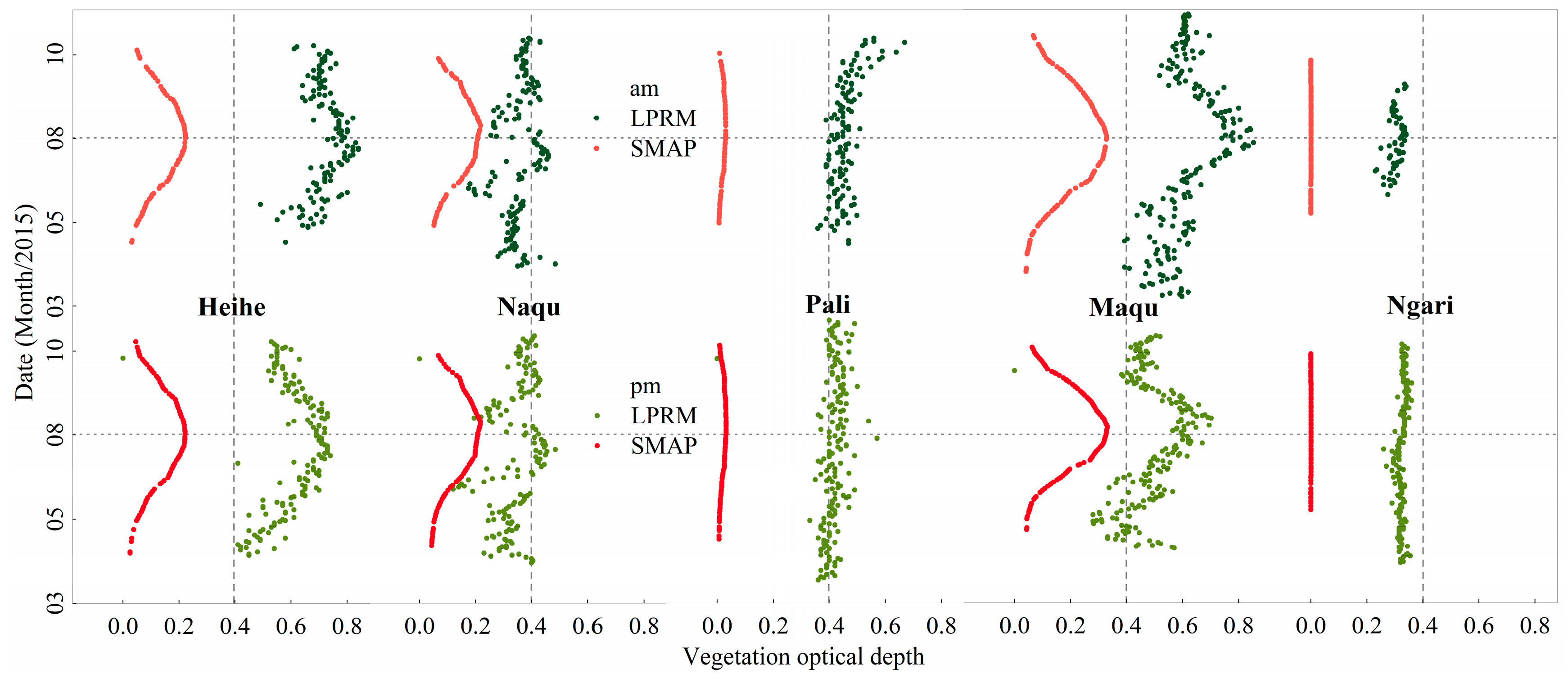
4.2. Vegetation Optical Depth

Microwave emission signals from vegetation must be removed from the total emissions to obtain the underlying soil emission signal, which is directly related to SM. Therefore, vegetation effects, which can be evaluated by two vegetation parameters, i.e., the effective scattering albedo ω and the optical depth τ, should be carefully considered so that accurate ground emissions can be obtained. In the five SM retrieval algorithms, the effective scattering albedo was set to a very small value, and the vegetation optical depth became the most influential factor.

According to Equation 4, the physical temperature can be eliminated from both sides of the equation by assuming that T_C=T_G. Then, the ground emissivity ε_g^p under polarization p (p = V/H) can be expressed as a function of the satellite observed emissivity ε^p (ε^p=TB^p/T_C), vegetation effective scattering albedo and transmissivity by rearranging the equation:

$${\mathsf{\epsilon }}_{\mathrm{g}}^{\mathrm{p}}=\frac{{\mathsf{\epsilon }}^{\mathrm{p}}-\left(1-{\mathsf{\omega }}^{\mathrm{p}}\right)\left(1-{\mathsf{\gamma }}^{\mathrm{p}}{}^2\right)}{{\mathsf{\gamma }}^{\mathrm{p}}\left({\mathsf{\omega }}^{\mathrm{p}}+{\mathsf{\gamma }}^{\mathrm{p}}-{\mathsf{\omega }}^{\mathrm{p}}{\mathsf{\gamma }}^{\mathrm{p}}\right)}$$

(5)

Based on Equation (5), Figure 11 presents the variations in the ground emissivity with different vegetation transmissivities γ at a certain remotely sensed emissivity, which is illustrated by different colors from blue (0.6) to red (0.9) based on simulations from the τ-ω model. For a fixed remotely sensed emissivity ε^p (same color), the simulated ground emissivity gradually increased as γ increased, corresponding to a decreasing τ. This relationship means that the ground emissivity would be overestimated for an underestimated τ under a certain observed brightness temperature when changing the physical surface temperature (that is, ε^p=TB^p/T_C, with ε^p changing between 0.6 and 0.9 here). Consequently, this situation produced an underestimated SM. The same result occurred when the effective scattering albedo was set to different values (ω=0, 0.03, 0.06, and 0.09).

The τ time series in the JAXA, FY3B, and SMOS-IC algorithms are not available online, so Figure 12 shows a comparison of the τ values for the SMAP and LPRM algorithms. Large differences existed among the two τ products. Specifically, the LPRM τ values were generally higher than those of SMAP, which can explain the full overestimations of the LPRM SM, as shown in Figure 3. The SMAP τ appeared as a nearly smooth hat-shaped curve on each in situ network and had continuous temporal and seasonal variability, with no obvious differences during the day or night. The distribution of τ better characterized areas with different vegetation coverage, and correspondingly higher values appeared in Heihe and Maqu, while correspondingly smaller values and poorer dynamic ranges occurred in Pali. The reason the SMAP τ adequately described the actual situation could be that the τ estimates based on the climatology of NDVI [47].

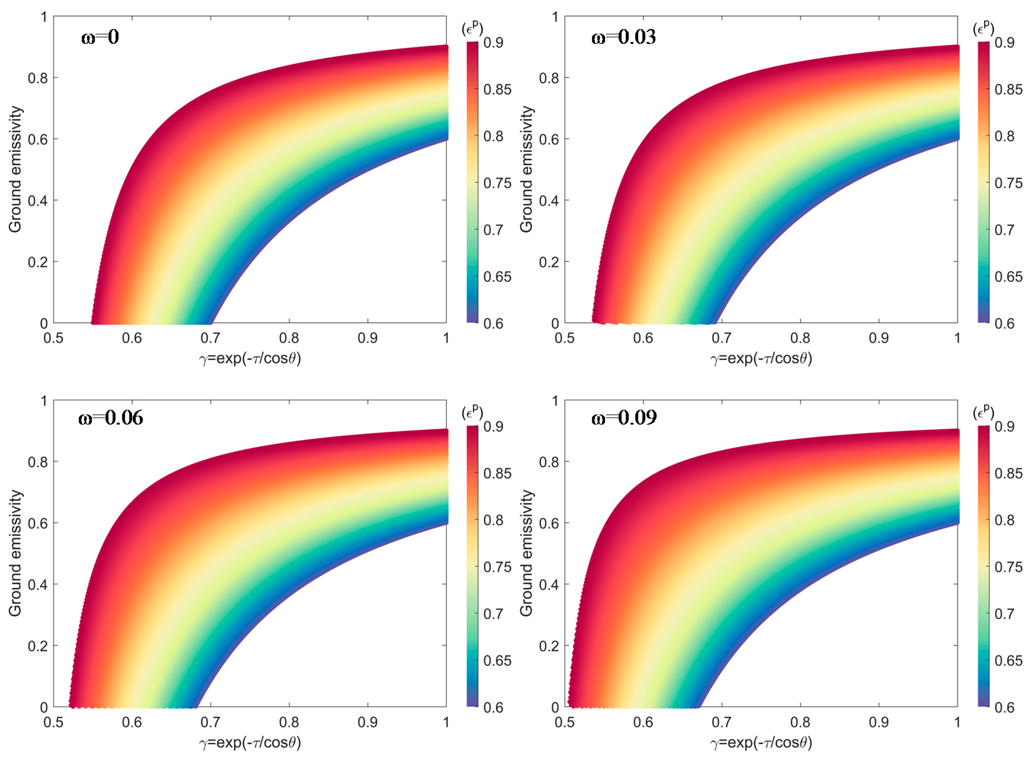
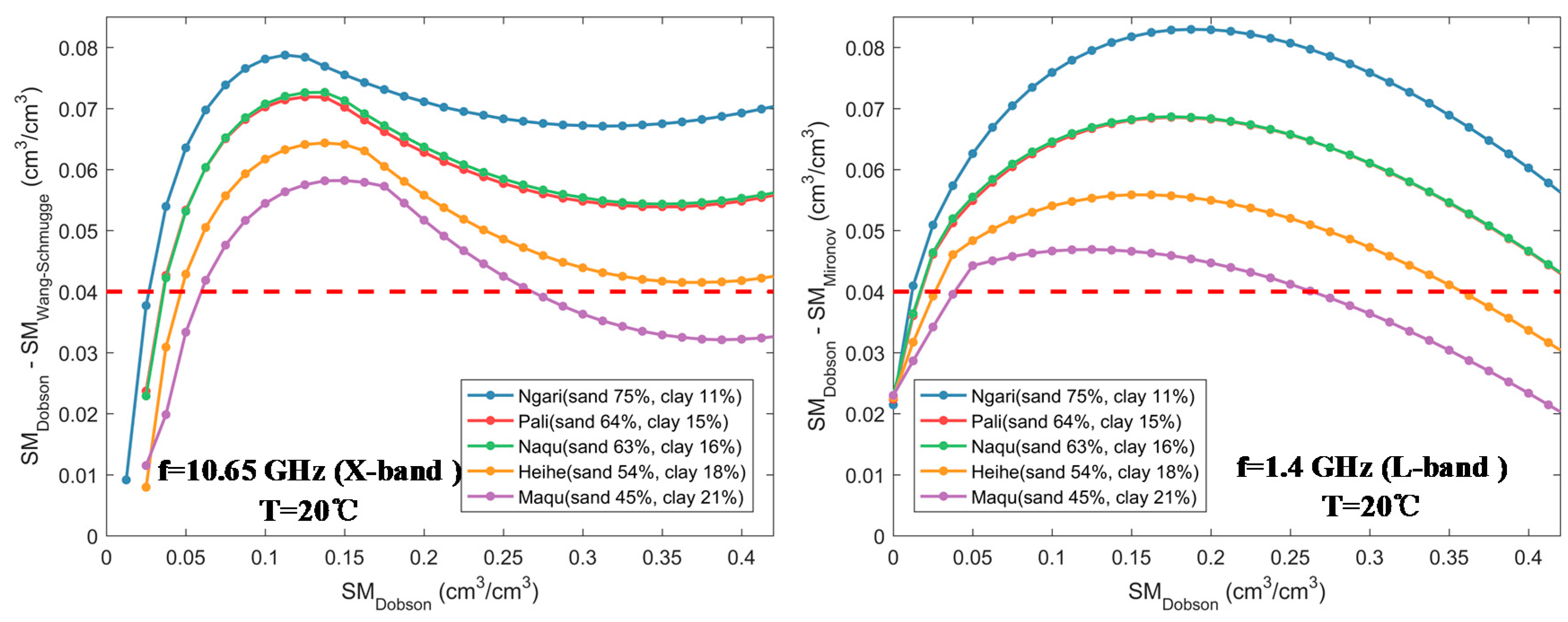
4.3. Soil Dielectric Mixing Model

As shown in Table 4, the Wang–Schmugge model [70] was adopted in the LPRM operational SM algorithm, the Dobson model [71] was adopted in the JAXA algorithm, and the newly developed Mironov model [72] was utilized in the SMOS-IC and SMAP SM algorithms. The FY3B SM was calculated from a relationship between the SM and a combination of two polarizations of rough surface emissivity without a soil dielectric constant model [12].

Table 5. Basic information of the three soil dielectric mixing models.

Model	Wang and Schmugge	Dobson	Mironov
Main inputs	Volumetric soil moisture, frequency, soil temperature, percentage of sand and clay, soil bulk density	Volumetric soil moisture, frequency, soil temperature, percentage of sand and clay, soil bulk density	Volumetric soil moisture, frequency, soil temperature, percentage of clay
Development time	1980	1985	2009
Type	Empirical	Semi-empirical	Physical
Consider bound soil water (BSW)	Yes	No	Yes

lists the basic information of these three soil-dielectric constant models. The Mironov model requires the fewest inputs, and the Wang–Schmugge and Dobson models require the same inputs. Undoubtedly, differences exist between the simulation results of these dielectric constant models [73,74].

To better analyze the influence of different soil dielectric constant models on the SM retrieval accuracy, five different soil texture conditions from five in situ networks (see Figure 1) were selected, and different soil dielectric constant models were used to retrieve SM under the same conditions. The Dobson and Wang–Schmugge models were used to retrieve SM in the X-band (10.65 GHz) under the same dielectric constant and soil texture, and their differences were calculated. In addition, the Dobson and Mironov models were used to retrieve SM in the L-band (1.4 GHz), and their differences were calculated (Figure 13).

The red horizontal dotted lines in Figure 13 are the reference accuracy (0.04 cm³ cm⁻³); the horizontal axis represents the estimated SM from the reference soil dielectric model, and the vertical axis represents the SM differences from using different soil dielectric constant models. The differences in the retrieval results between the Dobson and Wang–Schmugge models were relatively large, and the differences increased with increasing sand content. Based on Section 3.1, large differences existed between the JAXA and LPRM SM, especially in relatively arid regions with high sand content, which was consistent with the retrieval results of their corresponding dielectric constant models. The soil dielectric constant models may have influenced the retrieval accuracy of the JAXA and LPRM. Large differences were also found in the retrieval results from the Dobson and Mironov models in the L-band, and the differences were generally larger than the reference accuracy. Based on in situ experiments, Guo et al. [75] revealed that the Dobson model performs slightly better than the Mironov model at the L-band. However, Mialon et al. [76] found no superior performance from one model over the other after comparing the two-model outputs with in situ measurements. Therefore, the selection of a soil dielectric mixing model in soil moisture retrieval algorithms should be considered carefully, and more comparisons between different dielectric models must be conducted to obtain better SM products. SMAP may be better after using the Dobson model, although this product is sufficient under most conditions.

5. Conclusions

In this study, the performances of five passive microwave remotely sensed SM products (i.e., SMAP, SMOS-IC, FY3B, JAXA, and LPRM) were evaluated by direct and indirect comparison methods over the QTP and its surrounding areas. The direct comparisons focused on the performances of five SM products in five in situ networks (i.e., Heihe, Naqu, Pali, Maqu, and Ngari), and the comparison results were often more credible because the in situ measurements were generally regarded as the ground ‘true value’. Meanwhile, the indirect comparisons provided the uncertainty estimates of each pixel for each SM product, and the uncertainty results revealed the relative performances of each SM product, especially from a spatial perspective. Moreover, comparisons of the five SM algorithms and analyses for three important inputs (i.e., the physical surface temperature, vegetation optical depth, and dielectric mixing model) of SM retrieval models were conducted. The important findings gained at the regional scale are highlighted below.

Compared to the in situ SM measurements, SMAP had relatively large R and low RMSE and bias, especially in areas with relatively sparse vegetation (i.e., Naqu, Pali, Maqu, and Ngari). The direct comparison results also showed overestimations from the LPRM, slight underestimations and slightly noisy dynamics from SMOS-IC, underestimations from the JAXA, and good seasonality but poor absolute accuracy from FY3B. In addition, the inter-comparison results among the five SM products showed that SMAP had low uncertainties and its performance was less affected by climate and environmental variables. In contrast, SMOS-IC showed relatively high uncertainties. Other SM products (i.e., FY3B, JAXA, and LPRM) showed better performance in the mid-western QTP but poorer performance in the mid-eastern QTP.

The primary error sources of these passive microwave remotely sensed SM products were the retrieval algorithms and inputs. According to the analysis for SM retrieval algorithms and their inputs, the physical surface temperature may have affected the retrieval accuracy but was not the leading factor, especially for the SMSO-IC, JAXA, and LPRM SM. Correcting influences from the vegetation canopy was a key issue in the SM retrieval algorithms for FY3B, the JAXA, and the LPRM, especially in areas with relatively low and relatively high vegetation coverage. Moreover, the dielectric mixing model may have caused large performance differences between the JAXA and LPRM, and the use of the Dobson model may have improved the performance of SMAP.

Future work on remotely sensed SM data is recommended in two aspects. First, different SM retrieval algorithms should be characterized and evaluated under different climate and environmental conditions. In addition, several passive microwave remotely sensed SM products could be combined to fully utilize their capabilities.

References

1. Western, A.W.; Grayson, R.B.; Blöschl, G. Scaling of Soil Moisture: A Hydrologic Perspective. Annu. Rev. Earth Planet. Sci. 2002, 8, 149–180. [Google Scholar] [CrossRef]
2. Massari, C.; Brocca, L.; Moramarco, T.; Tramblay, Y.; Lescot, J.F.D. Potential of soil moisture observations in flood modelling: Estimating initial conditions and correcting rainfall. Adv. Water Resour. 2014, 74, 44–53. [Google Scholar] [CrossRef]
3. Hunt, K.M.R.; Turner, A.G. The Effect of Soil Moisture Perturbations on Indian Monsoon Depressions in a Numerical Weather Prediction Model. J. Clim. 2017, 30, 8811–8823. [Google Scholar] [CrossRef]
4. Cheng, S.; Guan, X.; Huang, J.; Mingxia, J.I. Analysis of Response of Soil Moisture to Climate Change in Semi-arid Loess Plateau in China Based on GLDAS Data. J. Arid Meteorol. 2013, 27, 4–19. [Google Scholar] [CrossRef]
5. Mcnairn, H.; Merzouki, A.; Pacheco, A. Monitoring Soil Moisture to Support Risk Reduction for the Agriculture Sector Using RADARSAT-2. IEEE J. Sel. Top. Appl. Earth Obs. Remote Sens. 2012, 5, 824–834. [Google Scholar] [CrossRef]
6. Lu, Z.; Qiang, D.; Islam, T.; Han, D. Error distribution modelling of satellite soil moisture measurements for hydrological applications. Hydrol. Process. 2016, 30, 2223–2236. [Google Scholar] [CrossRef]
7. Todisco, F.; Brocca, L.; Termite, L.; Wagner, W. Use of satellite and modeled soil moisture data for predicting event soil loss at plot scale. Hydrol. Earth Syst. Sci. 2015, 19, 3845–3856. [Google Scholar] [CrossRef]
8. Vyas, A.D.; Trivedi, A.J.; Calla, O.P.N.; Rana, S.S.; Raju, G. Passive microwave remote sensing of soil moisture. Int. J. Remote Sens. 1985, 6, 1153–1162. [Google Scholar] [CrossRef]
9. Jackson, T.J.; Cosh, M.H.; Bindlish, R.; Starks, P.J.; Bosch, D.D.; Seyfried, M.; Goodrich, D.C.; Moran, M.S.; Du, J.Y. Validation of advanced microwave scanning radiometer soil moisture products. IEEE Trans. Geosci. Remote Sens. 2010, 48, 4256–4272. [Google Scholar] [CrossRef]
10. Jackson, T.J., III. Measuring surface soil moisture using passive microwave remote sensing. Hydrol. Process. 1993, 7, 139–152. [Google Scholar] [CrossRef]
11. Wigneron, J.P.; Kerr, Y.; Waldteufel, P.; Saleh, K.; Escorihuela, M.J.; Richaume, P.; Ferrazzoli, P.; de Rosnay, P.; Gurney, R.; Calvet, J.C.; et al. L-band Microwave Emission of the Biosphere (L-MEB) Model: Description and calibration against experimental data sets over crop fields. Remote Sens. Environ. 2007, 107, 639–655. [Google Scholar] [CrossRef]
12. Liu, Q.; Du, J.Y.; Shi, J.C.; Jiang, L.M. Analysis of spatial distribution and multi-year trend of the remotely sensed soil moisture on the Tibetan Plateau. Sci. China 2013, 56, 2173–2185. [Google Scholar] [CrossRef]
13. Shi, J.C.; Jiang, L.M.; Zhang, L.X. A Parameterized Multi-Frequency-Polarization Surface Emission Model. IEEE Trans. Geosci. Remote Sens. 2005, 43, 2831–2841. [Google Scholar] [CrossRef]
14. Fujii, H.; Koike, T.; Imaoka, K. Improvement of the AMSR-E Algorithm for Soil Moisture Estimation by Introducing a Fractional Vegetation Coverage Dataset Derived from MODIS Data. J. Remote Sens. Soc. Jpn. 2009, 29, 282–292. [Google Scholar] [CrossRef]
15. Owe, M.; Jeu, R.D.; Holmes, T. Multisensor historical climatology of satellite-derived global land surface moisture. J. Geophys. Res. Earth Surf. 2008, 113, 196–199. [Google Scholar] [CrossRef]
16. Fernandez-Moran, R.; Al-Yaari, A.; Mialon, A.; Mahmoodi, A.; Al Bitar, A.; De Lannoy, G.; Rodriguez-Fernandez, N.; Lopez-Baeza, E.; Kerr, Y.; Wigneron, J. SMOS-IC: An alternative SMOS soil moisture and vegetation optical depth product. Remote Sens. 2017, 9, 457. [Google Scholar] [CrossRef]
17. Wigneron, J.P.; Jackson, T.J.; O’Neill, P.; De Lannoy, G.; de Rosnay, P.; Walker, J.P.; Ferrazzoli, P.; Mironov, V.; Bircher, S.; Grant, J.P.; et al. Modelling the passive microwave signature from land surfaces: A review of recent results and application to the L-band SMOS & SMAP soil moisture retrieval algorithms. Remote Sens. Environ. 2017, 192, 238–262. [Google Scholar] [CrossRef]
18. Wigneron, J.P.; Chanzy, A.; Kerr, Y.; Shi, J.C.; Cano, A.; Rosnay, P.D.; Escorihuela, M.J.; Mironov, V.; Demontoux, F.; Grant, J. Improved parameterization of the soil emission in L-MEB. IEEE Trans. Geosci. Remote Sens. 2011, 49, 1177–1189. [Google Scholar] [CrossRef]
19. Penna, D.; Tromp-van Meerveld, H.J.; Gobbi, A.; Borga, M.; Dalla Fontana, G. The influence of soil moisture on thresholds generation processes in an alpine headwater catchment. Hydrol. Earth Syst. Sci. 2011, 7, 689–702. [Google Scholar] [CrossRef]
20. Su, Z.; Wen, J.; Dente, L.; Velde, R.V.D.; Wang, L.; Ma, Y.; Yang, K.; Hu, Z. The Tibetan Plateau observatory of plateau scale soil moisture and soil temperature (Tibet-Obs) for quantifying uncertainties in coarse resolution satellite and model products. Hydrol. Earth Syst. Sci. 2011, 15, 2303. [Google Scholar] [CrossRef]
21. Dente, L.; Su, Z.; Wen, J. Validation of SMOS soil moisture products over the Maqu and Twente regions. Sensors Basel 2012, 12, 9965–9986. [Google Scholar] [CrossRef]
22. Zeng, J.; Li, Z.; Chen, Q.; Bi, H.; Qiu, J.; Zou, P. Evaluation of remotely sensed and reanalysis soil moisture products over the Tibetan Plateau using in-situ observations. Remote Sens. Environ. 2015, 163, 91–110. [Google Scholar] [CrossRef]
23. Cui, Y.; Long, D.; Hong, Y.; Zeng, C.; Zhou, J.; Han, Z.; Liu, R.; Wan, W. Validation and reconstruction of FY-3B/MWRI soil moisture using an artificial neural network based on reconstructed MODIS optical products over the Tibetan Plateau. J. Hydrol. 2016, 543, 242–254. [Google Scholar] [CrossRef]
24. Chen, Y.; Yang, K.; Qin, J.; Cui, Q.; Lu, H.; Zhu, L.; Han, M.; Tang, W. Evaluation of SMAP, SMOS, and AMSR2 soil moisture retrievals against observations from two networks on the Tibetan Plateau. J. Geophys. Res. Atmos. 2017, 122, 5780–5792. [Google Scholar] [CrossRef]
25. Ma, C.; Li, X.; Wei, L.; Wang, W. Multi-Scale Validation of SMAP Soil Moisture Products over Cold and Arid Regions in Northwestern China Using Distributed Ground Observation Data. Remote Sens.-Basel 2017, 9, 327. [Google Scholar] [CrossRef]
26. Zheng, D.; Wang, X.; Velde, R.V.D.; Ferrazzoli, P.; Wen, J.; Wang, Z.; Schwank, M.; Colliander, A.; Bindlish, R.; Su, Z. Impact of surface roughness, vegetation opacity and soil permittivity on L-band microwave emission and soil moisture retrieval in the third pole environment. Remote Sens. Environ. 2018, 209, 633–647. [Google Scholar] [CrossRef]
27. Kim, S.; Liu, Y.Y.; Johnson, F.M.; Parinussa, R.M.; Sharma, A. A global comparison of alternate AMSR2 soil moisture products: Why do they differ? Remote Sens. Environ. 2015, 161, 43–62. [Google Scholar] [CrossRef]
28. Tavella, P.; Premoli, A. Estimating the Instabilities of N Clocks by Measuring Differences of their Readings. Metrologia 1994, 30, 479. [Google Scholar] [CrossRef]
29. Ferreira, V.G.; Montecino, H.D.C.; Yakubu, C.I.; Heck, B. Uncertainties of the Gravity Recovery and Climate Experiment time-variable gravity-field solutions based on three-cornered hat method. J. Appl. Remote Sens. 2016, 10, 015015. [Google Scholar] [CrossRef]
30. Abbondanza, C.; Altamimi, Z.; Chin, T.M.; Gross, R.S.; Heflin, M.B.; Parker, J.W.; Wu, X. Three-Corner Hat for the assessment of the uncertainty of non-linear residuals of space-geodetic time series in the context of terrestrial reference frame analysis. J. Geodesy 2015, 89, 313–329. [Google Scholar] [CrossRef]
31. Awange, J.; Ferreira, V.; Forootan, E.; Khandu; Andam-Akorful, S.A.; Agutu, N.O.; He, X.F. Uncertainties in remotely sensed precipitation data over Africa. Int. J. Climatol. 2016, 36, 303–323. [Google Scholar] [CrossRef]
32. Qu, Y.; Zhu, Z.; Chai, L.; Liu, S.; Montzka, C.; Liu, J.; Yang, X.; Lu, Z.; Jin, R.; Li, X. Rebuilding a Microwave Soil Moisture Product Using Random Forest Adopting AMSR-E/AMSR2 Brightness Temperature and SMAP over the Qinghai–Tibet Plateau, China. Remote Sens.-Basel 2019, 11, 683. [Google Scholar] [CrossRef]
33. Valty, P.; de Viron, O.; Panet, I.; Van Camp, M.; Legrand, J. Assessing the precision in loading estimates by geodetic techniques in Southern Europe. Geophys. J. Int. 2013, 194, 1441–1454. [Google Scholar] [CrossRef]
34. Long, D.; Longuevergne, L.; Scanlon, B.R. Uncertainty in evapotranspiration from land surface modeling, remote sensing, and GRACE satellites. Water Resour. Res. 2014, 50, 1131–1151. [Google Scholar] [CrossRef]
35. Kang, S.; Xu, Y.; You, Q.; Flügel, W.A.; Pepin, N.; Yao, T. Review of climate and cryospheric change in the Tibetan Plateau. Environ. Res. Lett. 2010, 5, 15101. [Google Scholar] [CrossRef]
36. Liu, X.; Chen, B. Climatic warming in the Tibetan Plateau during recent decades. Int. J. Clim. 2015, 20, 1729–1742. [Google Scholar] [CrossRef]
37. Qin, J.; Yang, K.; Liang, S.; Guo, X. The altitudinal dependence of recent rapid warming over the Tibetan Plateau. Clim. Chang. 2009, 97, 321. [Google Scholar] [CrossRef]
38. Yang, K.; Ye, B.; Zhou, D.; Wu, B.; Foken, T.; Qin, J.; Zhou, Z. Response of hydrological cycle to recent climate changes in the Tibetan Plateau. Clim. Chang. 2011, 109, 517–534. [Google Scholar] [CrossRef]
39. Wang, B.; Bao, Q.; Hoskins, B.; Wu, G.; Liu, Y. Tibetan Plateau warming and precipitation changes in East Asia. Geophys. Res. Lett. 2008, 35, 63–72. [Google Scholar] [CrossRef]
40. Ge, Y.; Wang, J.H.; Heuvelink, G.B.M.; Jin, R.; Li, X.; Wang, J.F. Sampling design optimization of a wireless sensor network for monitoring ecohydrological processes in the Babao River basin, China. Int. J. Geogr. Inf. Sci. 2015, 29, 92–110. [Google Scholar] [CrossRef]
41. Jin, R.; Li, X.; Yan, B.; Li, X.; Luo, W.; Ma, M.; Guo, J.; Kang, J.; Zhu, Z.; Zhao, S. A Nested Ecohydrological Wireless Sensor Network for Capturing the Surface Heterogeneity in the Midstream Areas of the Heihe River Basin, China. IEEE Geosci. Remote Sens. Lett. 2014, 11, 2015–2019. [Google Scholar] [CrossRef]
42. Li, X.; Cheng, G.; Liu, S.; Xiao, Q.; Ma, M.; Jin, R.; Che, T.; Liu, Q.; Wang, W.; Qi, Y.; et al. Heihe Watershed Allied Telemetry Experimental Research (HiWATER): Scientific Objectives and Experimental Design. Bull. Am. Meteorol. Soc. 2013, 94, 1145–1160. [Google Scholar] [CrossRef]
43. Liu, S.; Li, X.; Xu, Z.; Che, T.; Xiao, Q.; Ma, M.; Liu, Q.; Jin, R.; Guo, J.; Wang, L. The Heihe Integrated Observatory Network: A basin-scale land surface processes observatory in China. Vadose Zone J. 2018, 17. [Google Scholar] [CrossRef]
44. Liu, S.M.; Xu, Z.W.; Wang, W.; Jia, Z.Z.; Zhu, M.J.; Bai, J.; Wang, J.M. A comparison of eddy-covariance and large aperture scintillometer measurements with respect to the energy balance closure problem. Hydrol. Earth Syst. Sci. 2011, 15, 1291–1306. [Google Scholar] [CrossRef]
45. Ma, M.; Che, T.; Li, X.; Xiao, Q.; Zhao, K.; Xin, X. A Prototype Network for Remote Sensing Validation in China. Remote Sens. Basel 2015, 7, 5187–5202. [Google Scholar] [CrossRef]
46. Yang, K.; Qin, J.; Zhao, L.; Chen, Y.; Tang, W.; Han, M.; Chen, Z.; Lv, N.; Ding, B. A Multi-Scale Soil Moisture and Freeze-Thaw Monitoring Network on the Third Pole. Bull. Am. Meteorol. Soc. 2013, 94, 1907–1916. [Google Scholar] [CrossRef]
47. O’Neill, P.E.; Chan, S.; Njoku, E.; Jackson, T.J.; Bindlish, R. Soil Moisture Active Passive (SMAP) Algorithm Theoretical Basis Document: Level 2 & 3 Soil Moisture (Passive) Data Products; Jet Propulsion Laboratory, NASA: Pasadena, CA, USA, 2015.
48. Ban, Y.; Li, S. China: Open access to Earth land-cover map. Nature 2015, 514, 434. [Google Scholar] [CrossRef]
49. Danielson, J.J.; Jeffrey, J. Delineation of drainage basins from 1 km African digital elevation data. In Proceedings of the Pecora Thirteen, Human Interactions with the Environment-Perspectives from Space, Sioux Falls, SD, USA, 20–22 August 1996. [Google Scholar]
50. Ying, X.U.; Gao, X.; Shen, Y.; Chonghai, X.U.; Shi, Y.; Giorgi, F. A Daily Temperature Dataset over China and Its Application in Validating a RCM Simulation. Adv. Atmos. Sci. 2009, 26, 763–772. [Google Scholar] [CrossRef]
51. Bindlish, R.; Cosh, M.H.; Jackson, T.J.; Koike, T.; Fujii, H.; Chan, S.K.; Asanuma, J.; Berg, A.; Bosch, D.D.; Caldwell, T. GCOM-W AMSR2 Soil Moisture Product Validation Using Core Validation Sites. IEEE J. Sel. Top. Appl. Earth Obs. Remote Sens. 2018, 11, 209–219. [Google Scholar] [CrossRef]
52. Jackson, T.J.; Bindlish, R.; Cosh, M.H.; Zhao, T.; Starks, P.J.; Bosch, D.D.; Seyfried, M.; Moran, M.S.; Goodrich, D.C.; Kerr, Y.H.; et al. Validation of Soil Moisture and Ocean Salinity (SMOS) Soil Moisture Over Watershed Networks in the U.S. IEEE Trans. Geosci. Remote Sens. 2012, 50, 1530–1543. [Google Scholar] [CrossRef]
53. Lu, Z.; Chai, L.; Zhang, T.; Cui, H.; Wang, J.; Li, W. Validation of SMOS soil moisture production in the Heihe River Basin of China. In Proceedings of the IEEE International Geoscience & Remote Sensing Symposium, Beijing, China, 10–15 July 2016. [Google Scholar] [CrossRef]
54. Lu, Z.; Chai, L.; Liu, S.; Cui, H.; Zhang, Y.; Jiang, L.; Jin, R.; Xu, Z. Estimating Time Series Soil Moisture by Applying Recurrent Nonlinear Autoregressive Neural Networks to Passive Microwave Data over the Heihe River Basin, China. Remote Sens.-Basel 2017, 9, 574. [Google Scholar] [CrossRef]
55. Rüdiger, C.; Calvet, J.C.; Gruhier, C.; Holmes, T.R.H.; Jeu, R.A.M.D.; Wagner, W. An intercomparison of ERS-Scat and AMSR-E soil moisture observations with model simulations over France. J. Hydrometeorol. 2009, 10, 431–447. [Google Scholar] [CrossRef]
56. Al-Yaari, A.; Wigneron, J.P.; Ducharne, A.; Kerr, Y.; Rosnay, P.D.; Jeu, R.D.; Govind, A.; Bitar, A.A.; Albergel, C.; Muñoz-Sabater, J. Global-scale evaluation of two satellite-based passive microwave soil moisture datasets (SMOS and AMSR-E) with respect to Land Data Assimilation System estimates. Remote Sens. Environ. 2014, 149, 181–195. [Google Scholar] [CrossRef]
57. Entekhabi, D.; Reichle, R.H.; Koster, R.D.; Crow, W.T. Performance metrics for soil moisture retrievals and application requirements. J. Hydrometeorol. 2010, 11, 832–840. [Google Scholar] [CrossRef]
58. Premoli, A.; Tavella, P. Revisited three-cornered hat method for estimating frequency standard instability. IEEE Trans. Instrum. Meas. 1993, 42, 7–13. [Google Scholar] [CrossRef]
59. Yilmaz, M.T.; Crow, W.T. Evaluation of assumptions in soil moisture triple collocation analysis. J. Hydrometeorol. 2014, 15, 1293–1302. [Google Scholar] [CrossRef]
60. Chin, T.M.; Gross, R.S.; Dickey, J.O. Multi-reference evaluation of uncertainty in Earth orientation parameter measurements. J. Geodesy 2005, 79, 24–32. [Google Scholar] [CrossRef]
61. Escorihuela, M.J.; Chanzy, A.; Wigneron, J.P.; Kerr, Y.H. Effective soil moisture sampling depth of L-band radiometry: A case study. Remote Sens. Environ. 2010, 114, 995–1001. [Google Scholar] [CrossRef]
62. Koster, R.D.; Guo, Z.C.; Dirmeyer, P.A.; Yang, R.Q.; Mitchell, K.; Puma, M.J. On the nature of soil moisture in land surface models. J. Clim. 2009, 22, 4322. [Google Scholar] [CrossRef]
63. Cui, H.; Jiang, L.; Du, J.; Zhao, S.; Wang, G.; Lu, Z.; Wang, J. Evaluation and analysis of AMSR-2, SMOS, and SMAP soil moisture products in the Genhe area of China. J. Geophys. Res. Atmos. 2017, 122, 8650–8666. [Google Scholar] [CrossRef]
64. Chakravorty, A.; Chahar, B.R.; Sharma, O.P.; Dhanya, C.T. A regional scale performance evaluation of SMOS and ESA-CCI soil moisture products over India with simulated soil moisture from MERRA-Land. Remote Sens. Environ. 2016, 186, 514–527. [Google Scholar] [CrossRef]
65. Leroux, D.J.; Kerr, Y.H.; Richaume, P.; Fieuzal, R. Spatial distribution and possible sources of SMOS errors at the global scale. Remote Sens. Environ. 2013, 133, 240–250. [Google Scholar] [CrossRef]
66. Mo, T.; Choudhury, B.J.; Schmugge, T.J.; Wang, J.R.; Jackson, T.J. A model for microwave emission from vegetation-covered fields. J. Geophys. Res. Ocean. 1982, 87, 11229–11237. [Google Scholar] [CrossRef]
67. Bindlish, R.; Jackson, T.; Cosh, M.; Koike, T.; Fuiji, X.; Jeu, R.D.; Chan, S.; Asanuma, J.; Berg, A.; Bosch, D. AMSR2 soil moisture product validation. In Proceedings of the IEEE International Geoscience & Remote Sensing Symposium, Fort Worth, TX, USA, 23–28 July 2017. [Google Scholar] [CrossRef]
68. Parinussa, R.M.; Wang, G.; Holmes, T.R.H.; Liu, Y.Y.; Dolman, A.J.; Jeu, R.A.M.D.; Jiang, T.; Zhang, P.; Shi, J. Global surface soil moisture from the Microwave Radiation Imager onboard the Fengyun-3B satellite. Int. J. Remote Sens. 2014, 35, 7007–7029. [Google Scholar] [CrossRef]
69. Holmes, T.R.H.; Jeu, R.A.M.D.; Owe, M.; Dolman, A.J. Land surface temperature from Ka band (37 GHz) passive microwave observations. J. Geophys. Res. 2009, 114. [Google Scholar] [CrossRef]
70. Wang, J.R.; Schmugge, T.J. An Empirical Model for the Complex Dielectric Permittivity of Soils as a Function of Water Content. IEEE Trans. Geosci. Remote Sens. 1980, GE-18, 288–295. [Google Scholar] [CrossRef]
71. Dobson, M.C.; Ulaby, F.T.; Hallikainen, M.T.; El-Rayes, M.A. Microwave Dielectric Behavior of Wet Soil-Part II: Dielectric Mixing Models. IEEE Trans. Geosci. Remote Sens. 1985, GE-23, 35–46. [Google Scholar] [CrossRef]
72. Mironov, V.L.; Kosolapova, L.G.; Fomin, S. Physically and mineralogically based spectroscopic dielectric model for moist soils. IEEE Trans. Geosci. Remote Sens. 2009, 47, 2059–2070. [Google Scholar] [CrossRef]
73. Laymon, C.A.; Crosson, W.L.; Jackson, T.J.; Manu, A.; Tsegaye, T.D. Ground-Based Passive Microwave Remote Sensing Observations of Soil Moisture at S-Band and L-Band with Insight into Measurement Accuracy. IEEE Trans. Geosci. Remote Sens. 2001, 39, 1844–1858. [Google Scholar] [CrossRef]
74. GÁlvez, J.F. Errors in soil moisture content estimates induced by uncertainties in the effective soil dielectric constant. Int. J. Remote Sens. 2008, 29, 3317–3323. [Google Scholar] [CrossRef]
75. Peng, G.; Shi, J.; Qiang, L.; Du, J. A New Algorithm for Soil Moisture Retrieval with L-Band Radiometer. IEEE J. Sel. Top. Appl. Earth Obs. Remote Sens. 2013, 6, 1147–1155. [Google Scholar] [CrossRef]
76. Mialon, A.; Richaume, P.; Leroux, D.; Bircher, S.; Al Bitar, A.; Pellarin, T.; Wigneron, J.; Kerr, Y.H. Comparison of Dobson and Mironov dielectric models in the SMOS soil moisture retrieval algorithm. IEEE Trans. Geosci. Remote 2015, 53, 3084–3094. [Google Scholar] [CrossRef]
Figure 1. In situ observation networks in the Qinghai-Tibet Plateau (QTP).
Remotesensing 11 00792 g001
Figure 2. Annual mean in situ soil temperature (green points) and mean in situ soil temperature of the five in situ observation networks (bold black lines).
Remotesensing 11 00792 g002
Figure 3. Time series that compare soil moisture active passive (SMAP), soil moisture and ocean salinity INRA-CESBIO (SMOS-IC), Fengyun-3B microwave radiation image (FY3B), Japan Aerospace Exploration Agency (JAXA) and land parameter retrieval model (LPRM) SM products with in situ measurements for 2015.
Remotesensing 11 00792 g003
Figure 4. Uncertainty results of the five SM products (ae) and (f) the total number of samples that were used in the three-cornered hat (TCH) method. The white areas indicate areas with no common samples or a sample size that was less than six.
Remotesensing 11 00792 g004
Figure 5. Spatial distribution of the SM products with the minimum uncertainty among the five SM products.
Remotesensing 11 00792 g005
Figure 6. Spatial patterns of several climate and environmental variables over the QTP. The mean values of the land-surface temperature (LST) and normalized difference vegetation index (NDVI) (0.25° × 0.25°) from April 2015 to July 2018 were used. PRE is the average annual precipitation from 2016 and 2017. The terrain complexity index (TCI), Clay, and Sand were relatively stable attributes for each period.
Remotesensing 11 00792 g006
Figure 7. Relationship between the selected variables (that is, PRE, TCI, NDVI, LST, Clay and Sand) and TCH-based uncertainty results. The boxplots show the median (black thick horizontal line), mean (black dot), 25th and 75th percentiles (top and bottom of the colored shaded box, respectively), and outlier ranges (edges of the top and bottom whiskers).
Remotesensing 11 00792 g007
Figure 8. Comparison of the R values between the polarization index (PI) or index of soil wetness (ISW) and in situ Ts for the morning and afternoon orbits from 2012 to 2016 in the five networks.
Remotesensing 11 00792 g008
Figure 9. Time series that compare the satellite-based Ts products with respect to the in situ Ts for the morning (nighttime) and afternoon (daytime) orbits for 2015 in five networks.
Remotesensing 11 00792 g009
Figure 10. The comparison of three performance metrics (including R and Bias) for the LPRM, SMOS-IC, and SMAP Ts data products for the morning (nighttime) and afternoon (daytime) orbits from 2012 to 2016 in five in situ networks.
Remotesensing 11 00792 g010
Figure 11. Relationship between the vegetation transmissivity and ground emissivity.
Remotesensing 11 00792 g011
Figure 12. Time series that compare the τ estimates from two SM models over the five in situ networks for 2015.
Remotesensing 11 00792 g012
Figure 13. Effect of different dielectric constant models on the soil moisture retrieval accuracy (left: soil moisture retrieval differences between the Dobson and Wang–Schmugge models under X-band conditions; right: differences between the Dobson and Mironov models under L-band conditions).
Remotesensing 11 00792 g013